Article

Optimized Spatial Gradient Transfer for Hyperspectral-LiDAR Data Classification

1
College of Information and Communication Engineering, Hunan Institute of Science and Technology, Yueyang 414000, China
2
Hyperspectral Computing Laboratory, Department of Technology of Computers and Communications, Escuela Politecnica, University of Extremadura, E-10003 Caceres, Spain
*
Author to whom correspondence should be addressed.
Remote Sens. 2022, 14(8), 1814; https://doi.org/10.3390/rs14081814
Submission received: 3 March 2022 / Revised: 25 March 2022 / Accepted: 5 April 2022 / Published: 9 April 2022
(This article belongs to the Topic Computational Intelligence in Remote Sensing)

Abstract

:
The classification accuracy of ground objects is improved due to the combined use of the same scene data collected by different sensors. We propose to fuse the spatial planar distribution and spectral information of the hyperspectral images (HSIs) with the spatial 3D information of the objects captured by light detection and ranging (LiDAR). In this paper, we use the optimized spatial gradient transfer method for data fusion, which can effectively solve the strong heterogeneity of heterogeneous data fusion. The entropy rate superpixel segmentation algorithm over-segments HSI and LiDAR to extract local spatial and elevation information, and a Gaussian density-based regularization strategy normalizes the local spatial and elevation information. Then, the spatial gradient transfer model and l 1 -total variation minimization are introduced to realize the fusion of local multi-attribute features of different sources, and fully exploit the complementary information of different features for the description of ground objects. Finally, the fused local spatial features are reconstructed into a guided image, and the guided filtering acts on each dimension of the original HSI, so that the output maintains the complete spectral information and detailed changes of the spatial fusion features. It is worth mentioning that we have carried out two versions of expansion on the basis of the proposed method to improve the joint utilization of multi-source data. Experimental results on two real datasets indicated that the fused features of the proposed method have a better effect on ground object classification than the mainstream stacking or cascade fusion methods.

1. Introduction

The development of remote sensing sensor technology makes it possible to obtain different types (e.g., hyperspectral image (HSI) and LiDAR) of remote sensing data in the same observation scene, which can capture a full range of identification information of ground coverings in the scene. A hyperspectral image (HSI) can provide rich spectral information for several materials; its high spectral resolution is conducive to distinguishing subtle spectral differences, and thus, making it widely used to identify and classify ground coverings [1,2,3]. However, the types of ground coverings are often complex, which leads to the phenomenon of the “same spectrum corresponds to multiple ground coverings” [4,5]. And HSI is a spatial flat spectral image degenerated from the real 3D spatial scene; thus, the height information of the observation area is lost. By contrast, LiDAR can obtain the digital surface model (DSM) information of the study area and is not easily restricted by weather or light [6,7]. Therefore, compared with a single data source, effectively combining HSI and LiDAR data and making full use of the complementary advantages of the two will greatly improve the accuracy of ground covering recognition [8,9].
In recent years, many supervised paradigm spectral classifiers have been developed to perform HSI classification tasks, such as the widely used support vector machine (SVM) [10,11], multinomial logistic regression classifier [12,13] and artificial immune network (AIN) [14]. Although these classifiers can effectively use the spectral information of HSI, they ignore the spatial context information of the pixels. To address this issue, many scholars have proposed a variety of classification methods based on spatial-spectral feature extraction [15,16,17]. In fact, these spectral-spatial classification methods are dedicated to extracting highly discriminative spatial-spectral features to improve classification accuracy further. For example, Wang et al. [18] design an extremely lightweight, non-deep parallel network (HyperLiteNet) that independently extracts and optimizes diverse and divergent spatial and spectral features. In [19], the adaptive sparse representation algorithm obtains the sparse coefficients of the multi-feature matrix for HSI classification, and these features reflect different kinds of spectral and spatial information. Furthermore, a Global Consistent Graph Convolutional Network(GCGCN) is proposed in [20], which uses graph topology consistent connectivity to explore adaptive global high-order neighbors to capture underlying rich spatial contextual information. The multiway attention mechanism has been successfully applied to HSI analysis due to the inspiration of the attention mechanism of the human visual system [21]. In addition to the above spatial-spectral classification methods, other useful techniques have been encouraged for hyperspectral classification, such as Markov random fields [22,23], collaborative representation [24,25] and edge-preserving filtering [26,27].
As the requirements for the classification of remote sensing scenes continue to increase, it is difficult for the single HSI data to meet the current interpretation task of ground coverings [28,29,30]. Although HSI data can provide rich diagnostic information (spectral features) for the identification of ground covering, it is limited by its low spatial resolution characteristics, resulting in a performance bottleneck in the classification model. LiDAR is a kind of digital image formed by digital surface model (DSM), which contains richer spatial detail information. In fact, many studies have demonstrated that the interpretation results of the gorund coverings are more accurate and stable by effectively combining the complementary strengths of HSI and LiDAR information [31,32]. For instance, Jia et al. was proposed a multiple feature-based superpixel-level decision fusion (MFSuDF) method for HSIs and LiDAR data classification. The motivation behind the MFSuDF is to considers the magnitude and phase information to obtain discriminative Gabor characteristics of the stacked matrix of HSI and LiDAR. Chen et al. [32] used dual convolutional neural networks (CNNs) to extract features from HSI and LiDAR data and a fully connected (FC) network to fuse the extracted features. These fusion models can extract robust features, but the fusion of HSI and LiDAR data still has many problems that should be explored in depth. Recently, the more popular fusion models adopt the method of features cascade or stacking, which ignores the difference in physical meaning and quantification range of different types of features and cannot encourage complementary information in the description of objects. Furthermore, the stacking mode may lead to information redundancy and Hughes phenomenon, especially in the case of small samples, overfitting may occur.
In the remote sensing community, the superpixel segmentation algorithm as a technique for clustering pixels based on dominant features (such as image color and brightness) has been widely used to extract the local spatial structure information of the pixels [33]. Some new technologies [34,35] that combine the spatial characteristics of superpixels have been proven successful in multi-source remote sensing data fusion tasks and improving the accuracy of ground object interpretation. Furthermore, Jiang et al. [36] introduced a superpixel principal component algorithm (SuperPCA) for HSI classification, which incorporated spatial context information into a superpixel to eliminate the difference of spatial projection between homogeneous regions. In [37], Zhang et al. constructed local-global features by improving the SuperPCA and reconstructed each pixel by exploiting the nearest neighbor pixels in the same superpixel to eliminate noise.
Strong isomerism of features limits the performance of feature fusion classification for heterologous data. The widely used stacking or cascading data fusion methods ignore the problems of different physical meanings, different data forms, and high feature dimensions describing the same scene with heterogeneous data. Therefore, the fusion method of stacking heterogeneous data cannot effectively achieve complementary information fusion. The basic motivation behind this paper is to use mathematical optimization to fuse the elevation information of single-band LiDAR with the spatial information of hyperspectral images for local feature fusion, which overcomes the high-order nonlinear phenomenon of multi-sensor data space and improves the information fusion performance of multi-dimensional heterogeneous feature discrimination of ground objects.
Specifically, the entropy rate superpixel segmentation algorithm over-segments HSI and LiDAR to extract local spatial and elevation information, and a Gaussian density-based regularization strategy normalizes the local spatial and elevation information. Then, the spatial gradient transfer model and l 1 -total variation minimization are introduced to realize the fusion of local multi-attribute features of different sources, and fully exploit the complementary information of different features for the description of ground objects. Finally, the fused local spatial features are reconstructed into a guided image, and the guided filtering acts on each dimension of the original HSI, so that the output maintains the complete spectral information and detailed changes of the spatial fusion features.
In addition, Figure 1a gives the part of the first principal component of the Houston data set. Figure 1b depicts LiDAR data, which contain distinct boundary and objects elevation information. Figure 1c simulates a fusion image obtaining by a stack-based fusion method. Figure 1d is the fusion result of the proposed OSGT algorithm. It can be seen from Figure 1 that the proposed OSGT method can capture more detailed spatial structure information than the stack-based fusion method. Specifically, the main contributions of the proposed OSGT method are summarized as follows.
  • We define homogeneous region fusion between PC and LiDAR data as a mathematical optimization problem and introduce the gradient transfer model to fuse spectral and DSM information from various superpixel blocks for the first time. It is found that the model can alleviate the heterogeneity of different sources of remote sensing data by optimizing the objective function.
  • The l 1 -total variation minimization is designed to fuse information between the PC and DSM within each superpixel block to accurately describe the observed details. It is found that the problem of HSI weak boundary affected by the weather can be effectively overcome.
  • The proposed OSGT algorithm can fully extract the complementary features in the homogeneous regions corresponding to HSI and LiDAR to further promote classification of ground coverings competitive methods.
The rest of this paper is organized as follows. The entropy rate superpixel (ERS) and guided filter (GuF) are reviewed in Section 2, and the proposed OSGF method for HSI and LiDAR data classification is introduced in Section 3. In Section 4, the experimental setup and results are described. Finally, the conclusions of our research are presented in Section 5.

2. Related Work

This section briefly describes some related algorithms, i.e., entropy rate superpixel (ERS), Guided Filtering (GuF). These algorithms play a relevant role in the design of the proposed method.

2.1. Entropy Rate Superpixel (ERS)

Entropy rate superpixel (ERS) [38] is an efficient graph-based over-segmentation method that generates a graph topology of N s connected subgraphs corresponding to homogeneous superpixels by maximizing the objective function containing an entropy rate term and a balancing term. The ERS method maps the image to a weighted undirected graph G = V , E , where the node set V and the edge weight E are the pixels of the image and the pairwise similarity given by the similarity matrix, respectively.
Consequently, the segmentation is formulated as a graph division problem, where V is divided into a series of disjoint sets S = [ S 1 , S 2 , , S N A ] , in which the intersection of any two subsets is empty, and the union of all subsets is equal to V. When selecting a subset A of E from G = V , E is finished, an undirected graph composed of N s subgraphs G = V , A is generated. The segmentation problem is formulated as maximizing the following objective function:
max A H A + λ B A s . t . A E
where H A is the entropy rate of the random walk encouraging uniform and compacting clusters, B A represents the balance term controlling clusters with similar sizes, and λ refers to the weight of the constrained entropy rate term and the balance term.

2.2. Guided Filtering

Guided filtering (GuF) [39] is an edge-preserving smoothing filter based on a local linear model. It has been successfully applied to various computer vision tasks, such as image edge smoothing [40], detail enhancement [41], and image fusion denoising [42]. The GuF typically uses a guided image to filter the input image. The output image contains the global features of the input image and the detailed changes of the guided image. The input image and the guided image are denoted as g and I, respectively. The output image is then defined as
t = Φ g f ( g , I , r , ξ )
where r is the filter window size, and ξ is the normalization parameter. g is a two-dimensional function whose output is linearly related to the guide input:
t i = a k I i + b k , i w k
where w k is a square window with radius r and the linear factors a k and b k are fixed values. The gradient of the output image is taken, t = a I . Therefore, if the guiding image has gradient property, the output image will also encourage the gradient. This is the reason why the GuF can smooth the background and maintain the high quality of the edge. The optimal linear factor a k and b k are obtained by minimizing the following cost function:
E a k , b k = i w k a k I k + b k g i 2 + ξ a k 2
where ε is the adjustment parameter of a k . The linear regression analysis method [43] is selected, and the optimal solution expression is written as:
a k = 1 w i w k I i g i μ k g k ¯ σ 2 + ξ
b k = g k ¯ a k μ k
where w is the number of pixels in w k , σ k 2 and μ k are the variance and mean of I in w k , respectively. Similarly, g k ¯ is the mean value of g in the window. Considering that pixel i may be contained in many windows, the linear coefficients calculated in different windows are divergent and, thus, the average value of a k and b k in the window centered on pixel i is obtained. The output image is then formulated as follows:
t i = 1 w k , i w a k I i + b k = a i ¯ I i + b i ¯

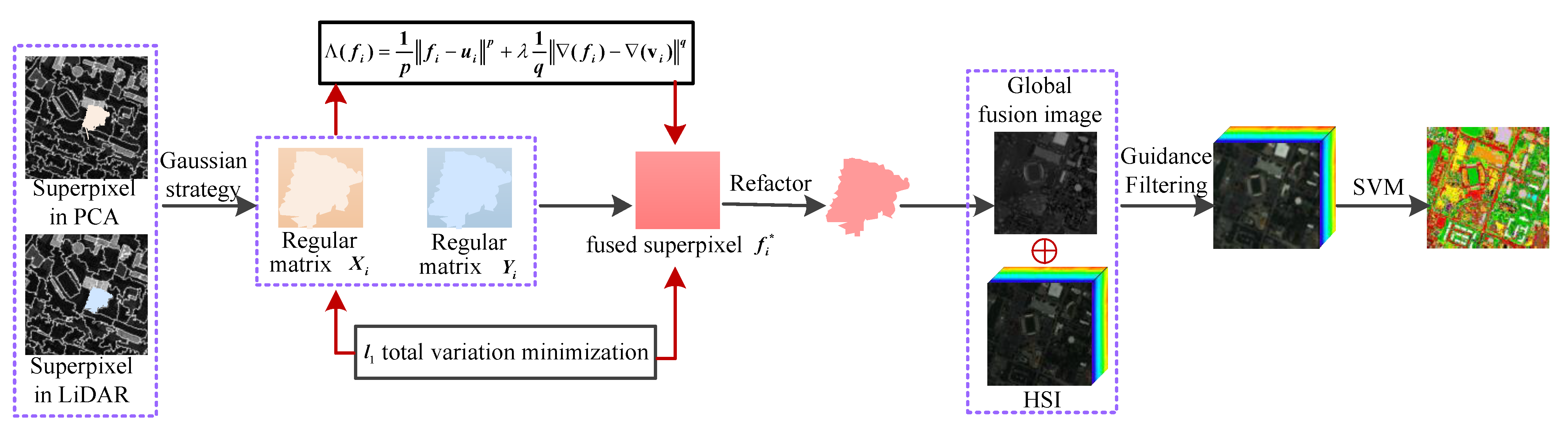
3. Proposed Approach

In this section, we introduce in detail the architectural steps of the proposed OSGT method for the classification of HSI and LiDAR data. The overall summary of the OSGT method is shown in Figure 2, A pseudo-code of our newly developed OSGT is given in Algorithm 1, and the specific steps are shown below.
Algorithm 1: OSGT.
Inputs: the HSI H; LiDAR data L; the number of superpixel N s ; the control parameter λ ; the training set T; and test set t;
Outputs: Classification result;
1. Superpixel Oversegmentation
    Obtain H s and L s based on PCA for H and L, by Equation (1)
For i = 1: N s
  Regularization strategy transforms S i and I i into X i and Y i
End
2. optimize spatial gradient transfer algorithm
For i = 1: N s
  Determine y i , by Equations (8)–(12)
  Obtain the fused superpixel blocks f i = y i + v i
  Reconstruct the fused superpixel blocks
End for
 Generate the fused image F
3. Classification
 Use F as the guided image to filter H, by Equation (13)
 Apply SVM to classify

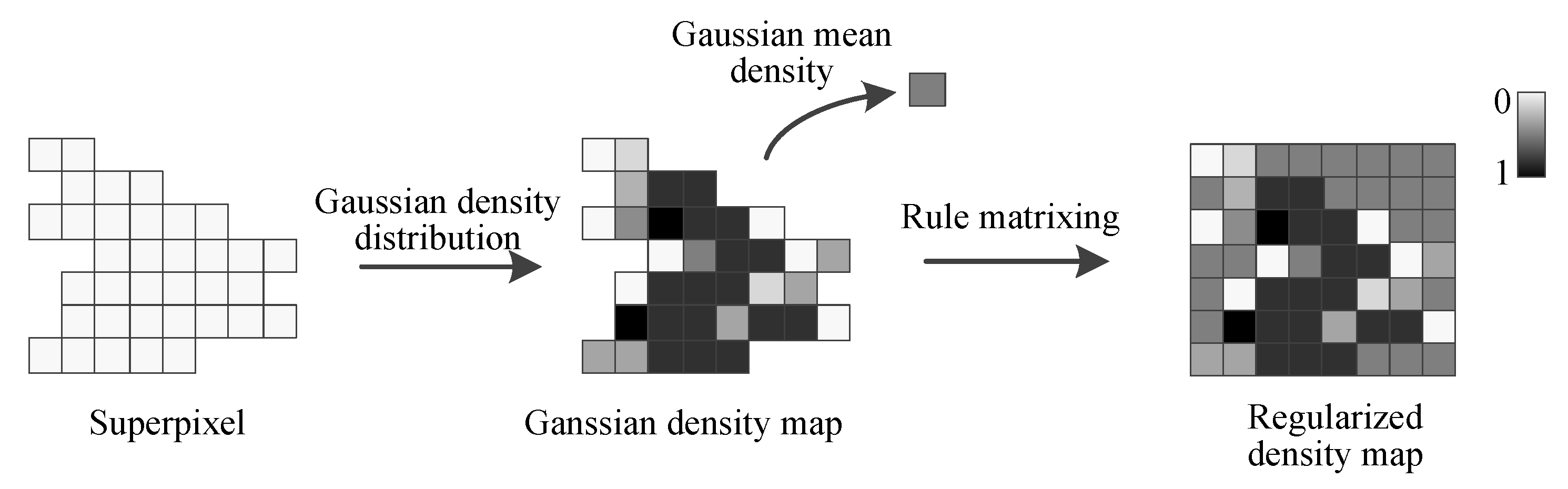
3.1. Oversegmentation

The hyperspectral cube H R M × N × B is composed of hundreds of continuous spectral bands. M, N, and B are the numbers of image rows, columns, and spectral channels, respectively. We have an observed 3D hyperspectral dataset in the 2D matrix form, H x D × B ( D = M × N ) , in which each column represents a pixel vector. Similarly, let L R M × N denote the LiDAR data.
The superpixel segmentation algorithm divides the target image into many disjointed regions. The samples in each region have the same or similar texture, color, and brightness. Assuming that the number of superpixels is N s , the oversegmented images of the first principal component of H and L are H s = S 1 , S 2 , , S N s and L s = I 1 , I 2 , , I N s , where S i and I i represent the superpixel blocks of H and L, respectively.
In order to alleviate the problem of the weak boundary of the super pixel, and the negative influence of the weak boundary on the edge gradient of the super pixel. As shown in Figure 3, a local space mean regularization strategy based on Gaussian density is designed. Specifically, the Gaussian kernel function calculates the samples density of S i and I i to describe the information between adjacent samples, and then averages the Gaussian density to fill the irregular S i and I i into regular matrix (i.e., X i and Y i , i 1 , 2 , , N s ), which not only maintains the spatial information of the superpixels but also avoids excessive edge gradient.

3.2. The Proposed OSGT Method

(1) Superpixel-guided gradient transfer fusion: The goal that the superpixel block X i of HSI and the superpixel block Y i of LiDAR fuse is to generate a fusion image that contains both spectral information and elevation features. X i , Y i and the fusion result can be regarded as grayscale images with a scale of m × n , and their column vector forms are represented by u i , v i , f i R m n × 1 , respectively.
HSI contains dense spectral information and scene detail information, and its high spectral resolution is conducive to distinguish the difference of different materials, which restricts the fusion result f i should have similar pixel intensity to u i . For the empirical error measured by l p norm should be as small as possible.
Λ 1 ( f i ) = 1 p f i u i p
The spatial dimension data of HSI is actually a 2-D image, but fusion image showing the 3-D spatial information of the observation area is necessary based on the importance of visual perception. The gray value of each point in the LiDAR image reflects the elevation information of the point and hence, we design fusion image f i to maintain similar pixel gradients instead of intensity to v i . For this, the error that is measured by l q norm must be as small as possible and is as follows:
Λ 2 ( f i ) = 1 q ( f i ) ( v i ) q
We define the fusion problem of superpixel blocks X i and Y i as minimizing the following objective function:
Λ f i = 1 p f i u i p + λ 1 q ( f i ) ( v i ) q
Here, the first term of the objective function is the data fidelity term, which indicates that f i should have the same pixel intensity as u i . The second term is the regularization term, which guarantees the same gradient information of f i and v i . λ is the control parameter that constrains the data fidelity term and regularization term. The objective function transfers the gradient information or elevation information of Y i to the corresponding position in X i .
(2) Total variation minimization: When the relationship between the fusion image and the constraint target is Gaussian, the l 2 norm is appropriate. However, We expect that the fusion result will be encouraged to retain more features of X i , as HSI exhibits texture features and spatial features, etc. besides spectral information. Therefore, most entries of f i and u i should be the identical. Only several entries are relatively large due to the gradient transfer of v i , so here ( p = 1 ) is the appropriate choice in this paper. In contrast, enhancing the sparsity of LiDAR image gradients can rely on minimizing LiDAR image l 0 , i.e., ( q = 0 ). However, the l 0 norm is NP-hard; thus, we replace l 0 with l 1 , implying that q = 1 .
Let y i = f i v i , the optimization problem (10) can be rewritten as:
y i = arg min y i j = 1 m n y i j u i j v i j + λ J y i
J y i = j = 1 m n i j y i = j = 1 m n i j h y i 2 + i j v y i 2
where a = a 1 2 + a 2 2 for every a = a 1 , a 2 R 2 . i j h and i j v represent the horizontal and vertical gradients of pixel j, respectively. The objective function in Equation (11) is solved directly using the proposed algorithm in [44]. y is obtained by optimizing Equation (11) using the technique of l 1 -TV minimization; thus, the target fusion outcome f i is decided by f i = y i + v i .
(3) Compute the global optimal solution: N s hyperspectral image superpixel blocks X i and LiDAR data superpixel blocks Y i have been obtained in Section 3.1. The total variable minimization method optimizes the objective function to fuse superpixel pairs. We denote by f 1 , f 2 , , f i , , f N s the column-vector form of the fusion result set of N s superpixel pairs, and the regular matrix form of the fusion result is expressed as r 1 , r 2 , , r i , , r N s . We perform superpixel refactor technology. Specifically, the position information of each pixel of S i and I i is used to select the pixel of the corresponding position in r i , and then an irregular superpixel block with the same size as the superpixel S i and I i is obtained. Finally, the N s inverted superpixel blocks are combined into a global fusion image F, where F R M × N .

3.3. Classification for HSI and LiDAR Data

One of the important factors affecting the filtering result is the guiding image, and the gradient of the output image obtained by guiding filtering is completely determined by the gradient of the guiding image.
In Section 3.2, the proposed method fuses HSI and LiDAR into a single-band image F. To some extent, it can be considered that the proposed method transfers the elevation information of the LiDAR data to the corresponding position of the HSI. Therefore, the fused image looks like the first principal component of HSI, but supplements the spatial detail information and cloud occlusion information to make the boundary contour of the object of interest more complete.
We choose the fusion image F as the guiding image, and the original hyperspectral image H as the guiding filter input. Specifically, given the guiding filter window radius r, and the filter ambiguity ξ , we can obtain the following filtering equation:
F H = G F r , ξ H , F
The filtered output can preserve the overall features of the input image and the detailed changes of the guided image through the adjustment of related parameters. It is worth mentioning that the samples in Figure 4 are closer to each other than the samples in Figure 4a, which indicates that the samples in Figure 4b have a higher quality. The structure transfer characteristics of the guided filtering can eliminate edge blocking effects and enhance the ability of feature expression. The filtered features are passed through the SVM classifier to obtain the final classification result.

3.4. Extension Method

In this section, the two extended methods we propose are implemented from the perspectives of band fusion to reduce data dimensionality and multi-branch to enrich detailed information, respectively.
(1) We propose an optimized spatial gradient fusion algorithm based on band grouping cooperation aiming to reduce dimensionality while maintaining the physical properties of the data. Since the adjacent bands of hyperspectral image are redundant and highly correlated, the fusion operation can reduce dimensionality and reduce image noise. Specifically, BG-OSGT does not change the main algorithm structure of OSGT. It divides and fuses the filter result graph obtained by the OSGT algorithm instead of directly using SVM for classification. In Section 3.3, the filtering feature map is determined, and in this section we divide it into K adjacent band subsets in the spectral dimension. The kth ( k ( 1 , , K ) ) group is defined as follows:
P k = ( x k , , x k + B / K ) , if k + B / K B ( x k , , x B ) , otherwise
where x = ( x 1 , , x B ) R B × D denotes the filtering feature map containing B feature vectors and D pixels, and then B / K represents an integer not greater than B / K . Then, the adjacent bands in the kth group are fused by the mean value strategy, that is, the calculation formula of the fusion feature R k of the kth group is:
R k = i = 1 N k P k i N k
where P k i is the ith band in the kth band grouping and N k is the total number of bands in the kth band grouping.
By taking advantage of the each grouping feature, the decision fusion strategy can effectively increase the classification accuracy. Specifically, we fused the label information of each test pixel predicted by different groups. The final classification map is determined by
F c = arg max c = 1 , , G i = 1 K χ ( l i = c )
where F c is the class label from one of the G possible classes for the test pixel, χ represents the indicator function. Algorithm 2 describes the overall process of the method.
Algorithm 2: BG-OSGT.
Inputs:H; L; N s ; λ ; T; and t;
Outputs: Classification result;
1. Superpixel Oversegmentation
 Obtain H s and L s based on PCA for H and L, by Equation (1)
For i = 1: N s
  Regularization strategy transforms S i and I i into X i and Y i
End
2. optimize spatial gradient transfer algorithm
For i = 1: N s
  Determine y i , by Equations (8)–(12)
  Obtain the fused superpixel blocks f i = y i + v i
  Reconstruct the fused superpixel blocks
End for
 Generate the fused image F
3. Classification
 Use F as the guided image to filter H, by Equation (13)
 Apply band grouping strategy to the filtered result
 Multi-branch classification and decision fusion by using SVM
(2) The first principal component of hyperspectral image contain most of the main information, the OSGT algorithm fuses the first principal component of hyperspectral image with LiDAR data. However, if only the first principal component is encouraged, some details may be lost. As shown in Figure 5, there is still information available in the second and third principal components. Therefore, the multi-branch optimize spatial gradient transfer (MOSGT) decision fusion framework is proposed, which aims to enrich image details and corner pixels. Specifically, MOSGT uses the OSGT algorithm to fuse the first three principal components of hyperspectral image with LiDAR data to generate three fused images. Then, the fused feature maps are used as guide images to filter the original hyperspectral image to obtain filtered feature maps, which can make full use of the complementary information between different guide images. In this section, we still use the majority voting decision strategy due to its insensitivity to inaccurate estimates of posterior probabilities.
Algorithm 3: MOSGT.
Inputs:H; L; N s ; λ ; T; and t
Outputs: Classification result;
1. Extract the first three principal components M i p c of H, where i = 1 , 2 , 3
2. Oversegmented M i p c and L by using ERS method, and then generate oversegmented maps S i p c and L s
3. Apply Gaussian regularization strategy to S i p c and L s
4. Fusion of S i p c and L s according to (8)–(12)
5. Obtain the fused superpixel blocks f i = y i + v i
6. Reconstruct the fused superpixel blocks
7. Generate the fused image set F i
8. Use F i as the guided images to filter H, by Equation (13)
9. Classify filtering feature images and decision fusion strategy.

4. Experimental Results
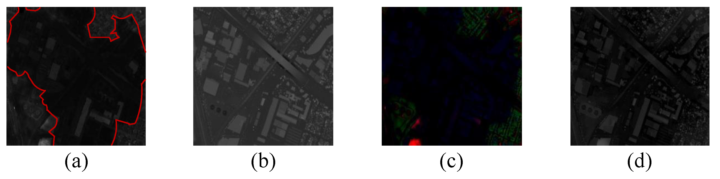
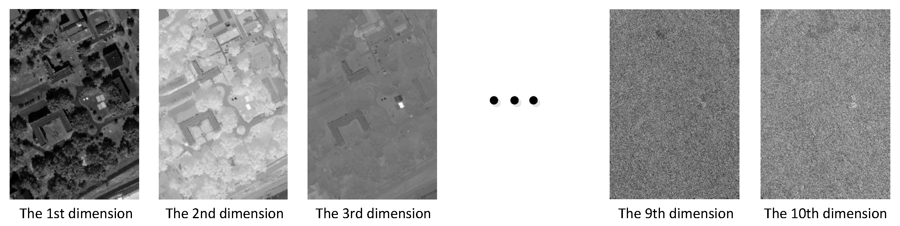
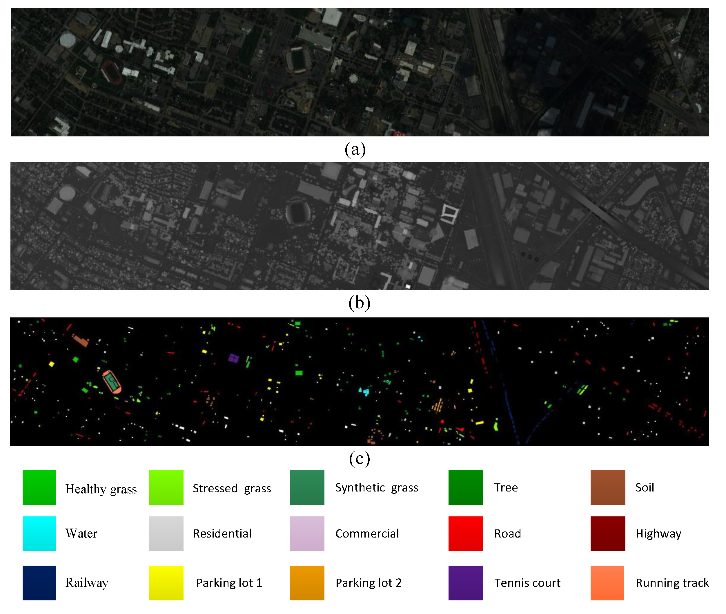
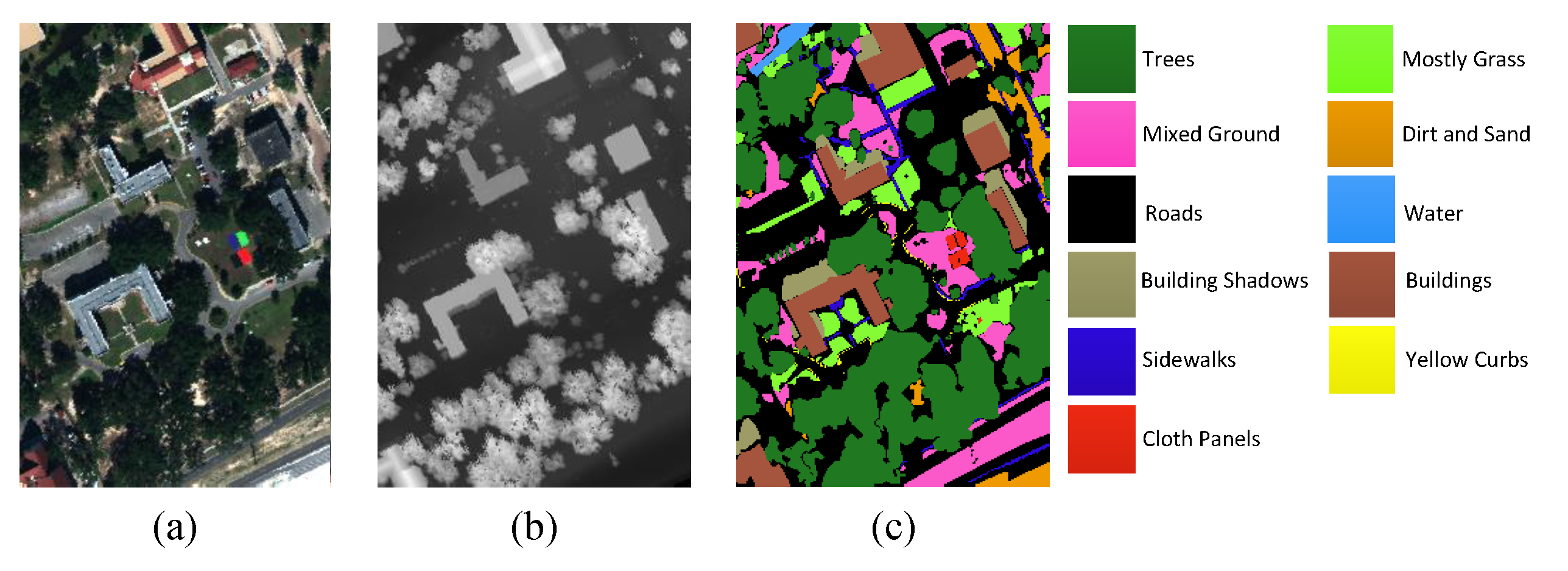
4.1. Datasets

(1) Houston Dataset: The University of Houston image is over the University of Houston campus and surrounding area [9]. It is composed of HSI and LiDAR data, both of which have a spatial dimension of 349 × 1905 and spatial resolution is 2.5 m per pixel. The HSI used in the experiments contains 144 bands, and the wavelength ranges from 380 to 1050 nm. Figure 6 illustrates the false-color composite of the University of Houston image, a grayscale image of the LiDAR data, and the corresponding reference data—there are 15 different classes. The exact numbers of samples for each class are reported in Table 1.
(2) MUUFL Gulfport Dataset: The MUUFL Gulfpor image is over the University of Southern Mississippi Gulfport Campus [45,46]. The HSI has a spatial dimension of 325 × 337 and 72 spectral bands. After discarding 8 bands contaminated by noise, the image contains 64 bands. Furthermore, considering the invalid area of the scene, the original hyperspectral is cropped to 325 × 220 × 64 as the new data set. The false-color composite of MUUFL Gulfport, a grayscale image of the LiDAR data, and the corresponding reference data are shown in Figure 7. The nine land-cover classes are described in detail in Table 1.

4.2. Quality Indexes

In order to objectively evaluate the performance of the proposed methods (i.e., the OSGT, BG-OSGT, and MOSGT method), the experiments adopt three objective indicators, i.e., overall accuracy (OA), average accuracy (AA), and Kappa coefficient. OA refers to the probability that the classification result is consistent with the ground truth. AA considers the imbalance of the number of samples in different classes. Kappa represents the consistency between the classification results and the true classes of ground objects—the greater its value, the more accurate the classification result. To eliminate the influence of randomness, the results of all quantitative indicators are averages of ten results.

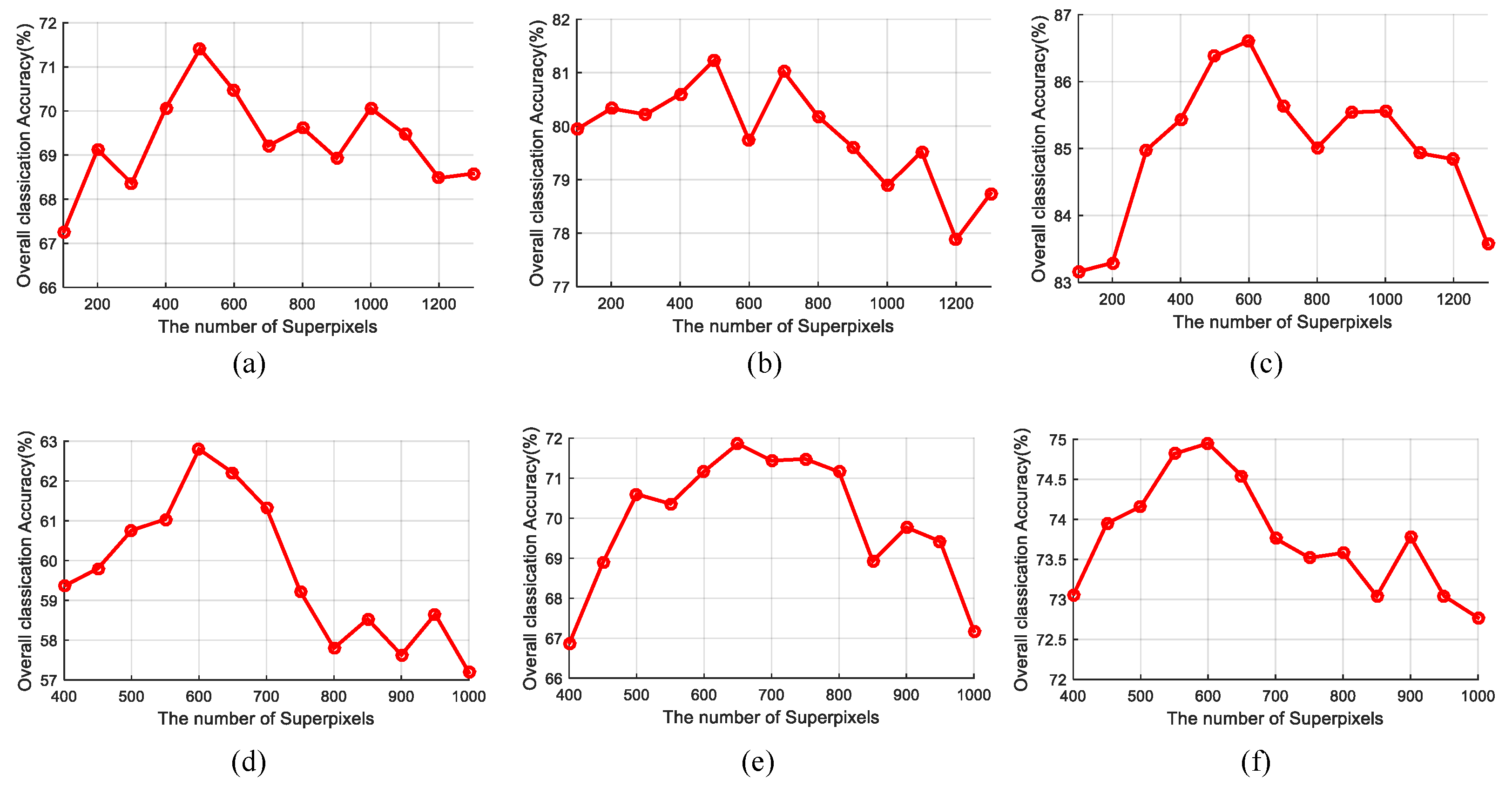
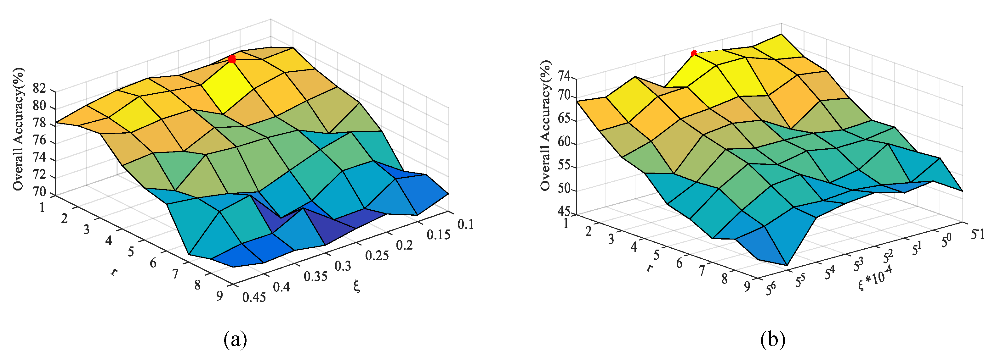
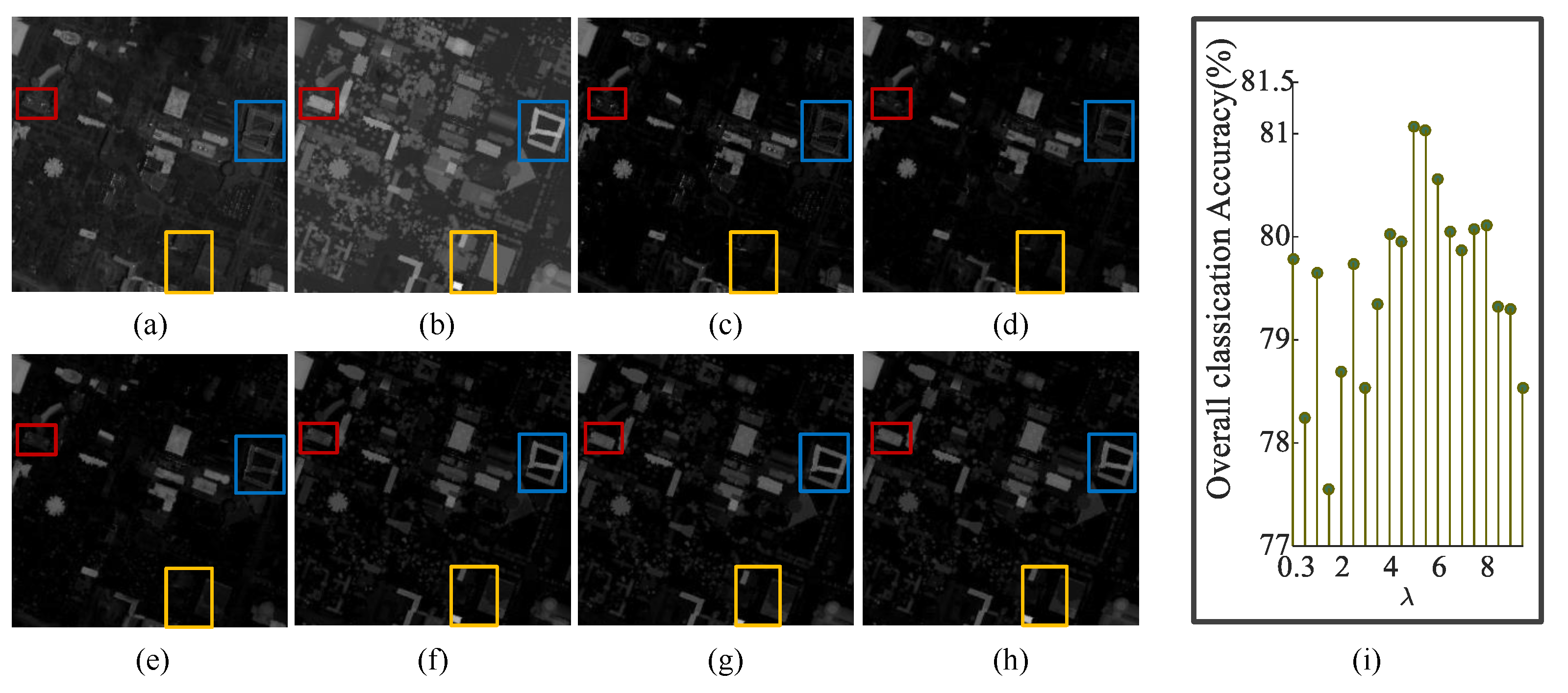
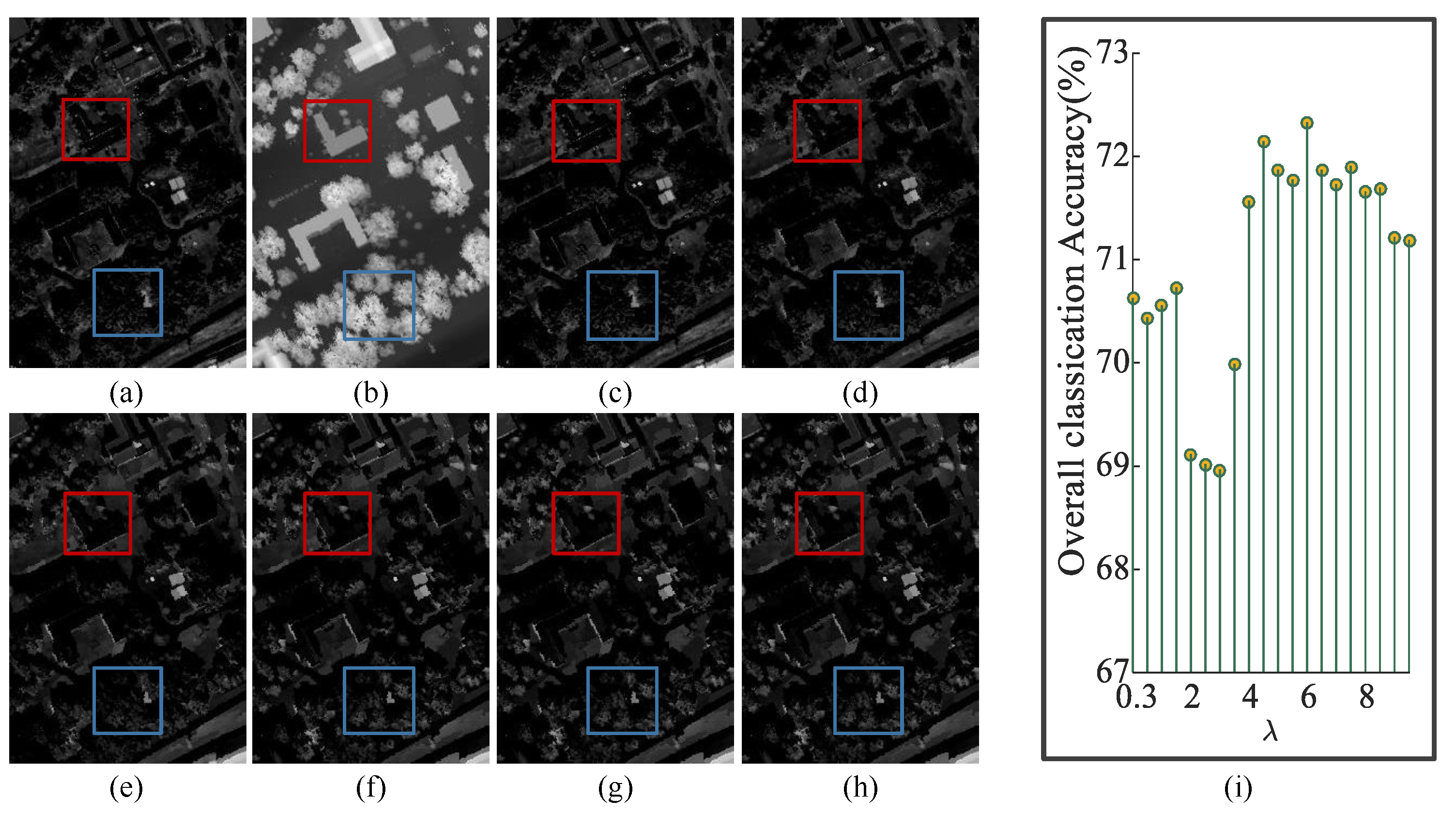
4.3. Analysis of Parameters Influence

(1) Effect of number of superpixels: In this section, the effect of the number of superpixels on the performance of the proposed OSGT method is evaluated on the Houston and MUUFL Gulfport dataset. As shown in Figure 8, it can be seen that the performance of the proposed OSGT method decreases significantly when the number of superpixels is less than 500 or 600. However, when the number of superpixels is higher than 500 or 600, the classification accuracy slowly decreases. The primary reason is that the large homogeneous region (small number of superpixels) causes the oversegmented map to contain many boundary superpixels that need to be further segmented. And a smaller homogeneous region (large number of superpixels) leads to poor discrimination of features in the regions. Furthermore, a small number of superpixels can reduce the computational cost. Therefore, the number of superpixels is fixed to 500 for the Houston data set and 650 for the MUUFL Gulfport dataset in this work.
(2) Effect of window radius and ambiguity of the GuF: The influence of two parameters, i.e., the window radius r and ambiguity ξ of the guided filtering, are analyzed on the above datasets. Figure 9 illustrates the OA versus r and ξ on different datasets; OA decreases significantly as the window radius r increases. When r and ξ are very small, useful detailed information and corner pixels can be determined. For the Houston dataset, the proposed OSGT method achieves the highest OA when r is set to 2 and ξ is equal to 0.2. For the MUUFL Gulfport dataset, when r = 1 and ξ = 2.5 × 10 3 , the OSGT method obtains satisfactory classification accuracy.
(3) Effect of free parameter: The free parameter λ that controls the data fidelity and regularization terms of the objective function impacts the performance of the proposed OSGT method. Figure 10 illustrates the visualized fusion results and the quantitative index OA under different free parameters for the Houston dataset. As λ increases, the fusion image contains the more abundant elevation information of LiDAR data. However, when the λ is too high, a small amount of detailed information disappears in the fused image because they only belong to HSI. Our goal is to retain more information existing in HSI, so that the fusion image still resembles HSI. When λ is set to approximately 5, the fusion result retains the small-scale details of the edge of HSI and adds the elevation feature of the ground object. Similarly, Figure 11 reflects that the parameter λ can balance the detailed appearance information and elevation features of the MUUFL Gulfport dataset. When λ is equal to approximately 6, the fusion result is satisfactory.

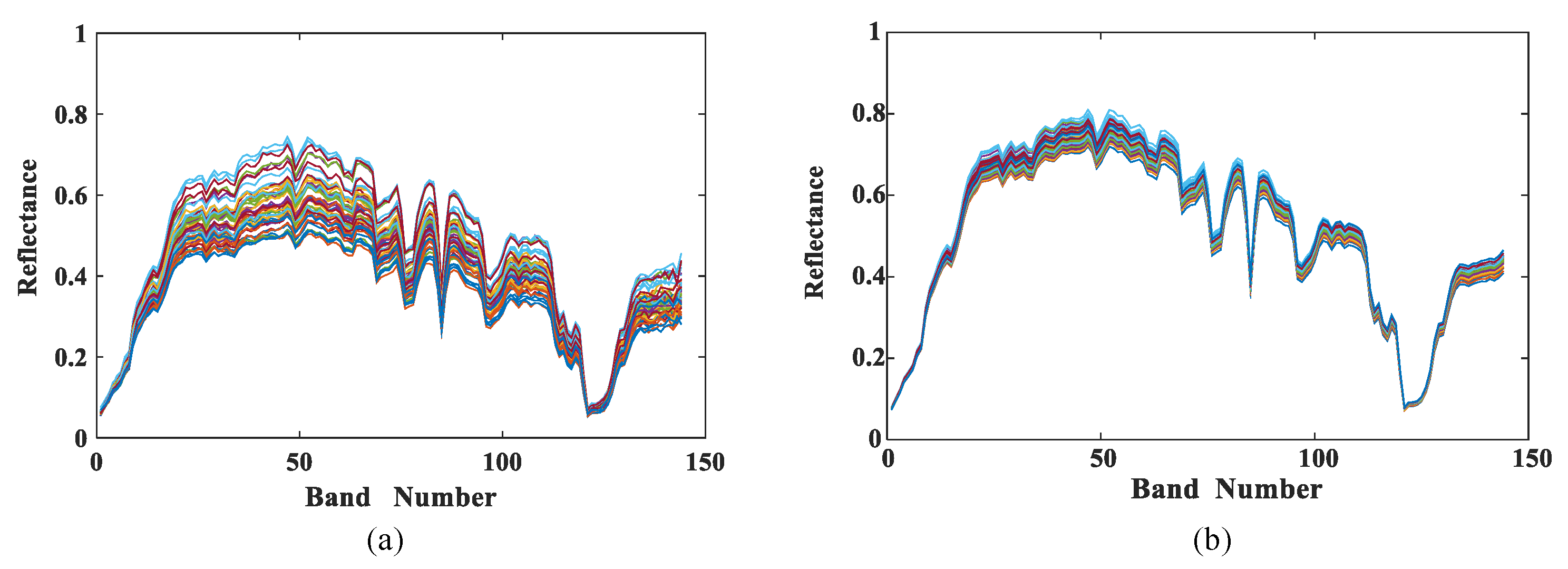
4.4. Analysis of Auxiliary between HSI and LiDAR Data

In this section, the auxiliary effect of LiDAR data on HSI is analyzed on the Huston and MUUFL Gulfport datasets. In this experiment, the numbers of training and test samples are selected to the same as those presented in Table 1. SVM-HSI indicates that SVM classifies the original HSI. G-PCA and G-LiDAR indicate, respectively, that the first PC and the LiDAR data are used as a guide image to filter the original HSI. G-PL represents that LiDAR data is stacked as a band of HSI to form a new dataset, and then the new dataset is then filtered using the first PCs as a guide image. For ensuring the experiment’s validity, a spatial mean strategy based on Gaussian density is used for the guide images of the comparison methods. The super-segmented map of the guide image is subjected to Gaussian density mean filtering in the homogenous region. The experiment is respectively performed on the Houston and MUUFL Gulfport datasets to verify the classification performance of the proposed OSGT method.
As shown in Figure 12, the SVM-HSI leads to an unsatisfactory classification accuracy (OA = 76.32%), indicating that the original HSI contains fuzzy boundary information and noise. Therefore, the classification performance of HSI without any preprocessing must often be improved. Furthermore, the classification accuracy of G-PCA and L-PCA are similar. This phenomenon indicates that the small-scale detail information of the PCA and the elevation attributes of the ground features encouraged by LiDAR can be transferred to the output of the filter as the structure of the guide image. Although their classification performance is similar, the features used to guide filtering differ. G-PL does not significantly improve classification performance because although HSI and LiDAR data are combined into cascaded data, the stacking of two different information expression forms ignores the feature heterogeneity. The proposed OSGT method in this paper fuses multi-source data from the perspective of mathematical optimization, causing the fusion result to contain both appearance detail information and elevates the features of the ground objects so that the guide image structure information is closer to the ground truth value.

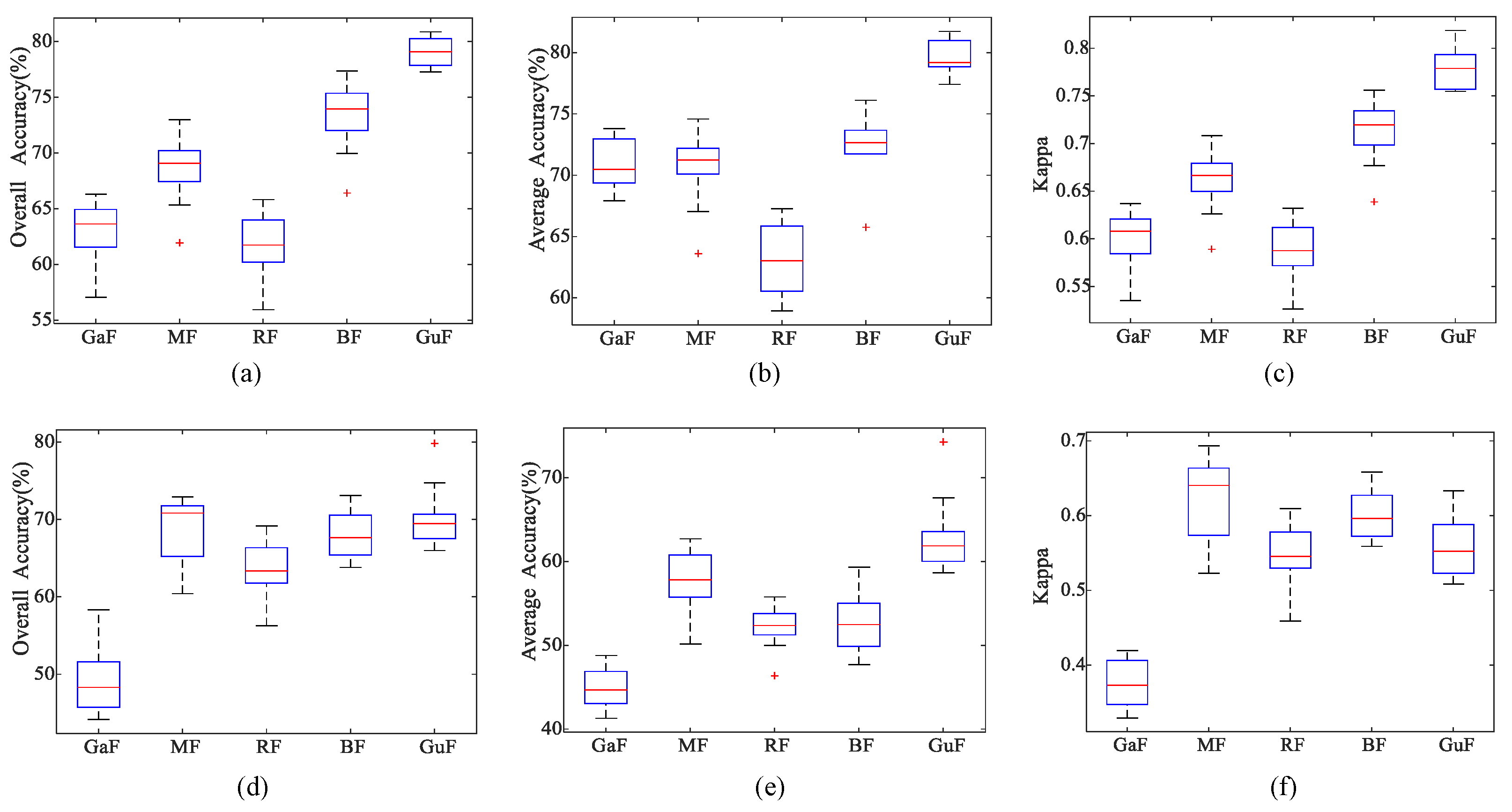
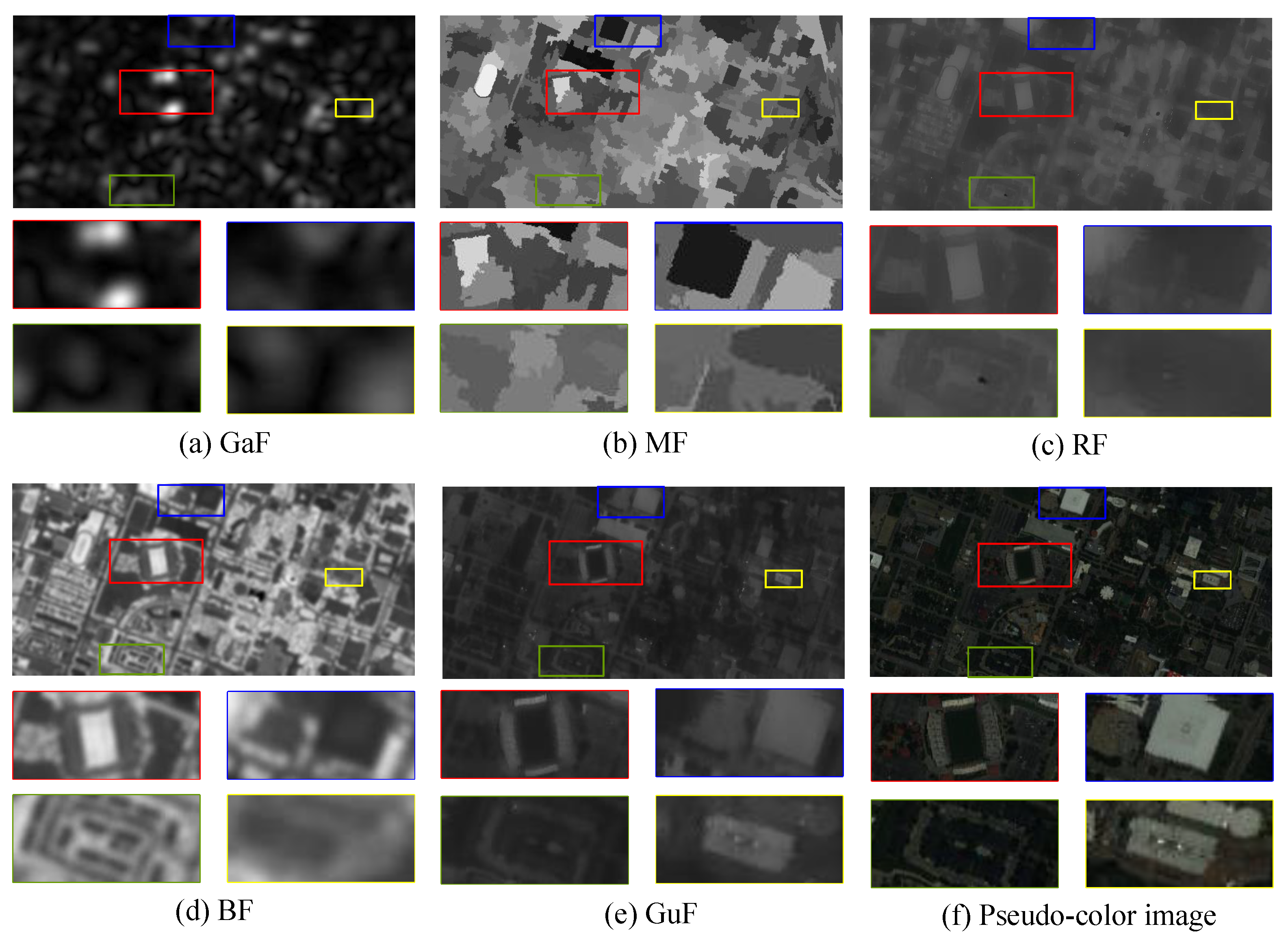
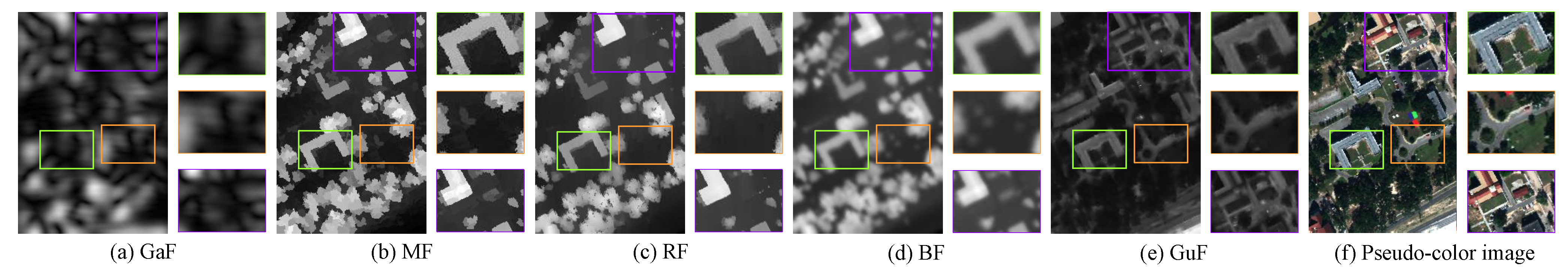
4.5. Effect of Filtering Method

In this section, we analyze the impact of different filtering methods on the performance of the proposed OSGT method, by comparing five widely used filtering methods: Gabor filtering (GaF) [47], mean filtering (MF) [48], recursive filtering (RF) [49], bilateral filtering (BF) [50] and guided filtering (GuF).
Figure 13 reports the classification accuracy of the above filtering methods. The cascaded data combined with HSI and LiDAR data are used as the filtering input to test the performance of these filtering methods in terms of extraction of structural information for multi-source data. The relevant parameters adopt the default parameter settings; the GuF parameters are the same as the parameters of the proposed OSGT method. Additionally, as shown in Figure 14 and Figure 15, it can be seen that the GuF method pays more attention to edge detail information and effectively retains the overall spatial features of the input image. Although the accuracy of the MF is slightly higher than GuF on the MUUFL Gulfport data set, its filtering performance of the MF on the Houston data set is significantly worse.

4.6. Effect of Local Features and Global Features

In this section, the influence of global and local features on image fusion is analyzed in Table 2. The operation of LiDAR images without superpixel processing directly as a guide map is denoted as NSL and the operation of the PCs images without superpixel processing directly as a guide map is denoted as NSP. PCL-GTF and P C 3 L-GTF indicate that the first PC and the first three PCs, respectively, are fused with the LiDAR data by global gradient transfer. It can be observed from Table 2 that the proposed OSGT method achieves the highest classification accuracy in terms of OA, AA, and Kappa. It is advantageous to fuse the PCs image and LiDAR data in a homogeneous region because the local explicit correlation of superpixels and the homogeneous regions of HSI can be used as the spatial structure information of spatial-spectral classification, enriching the fusion results.

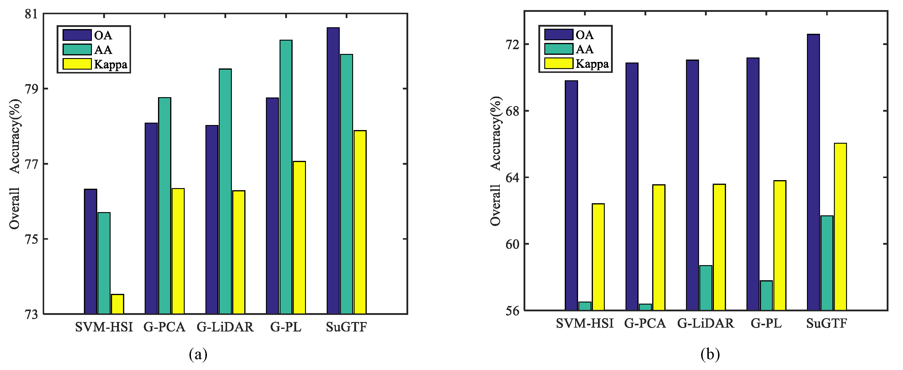
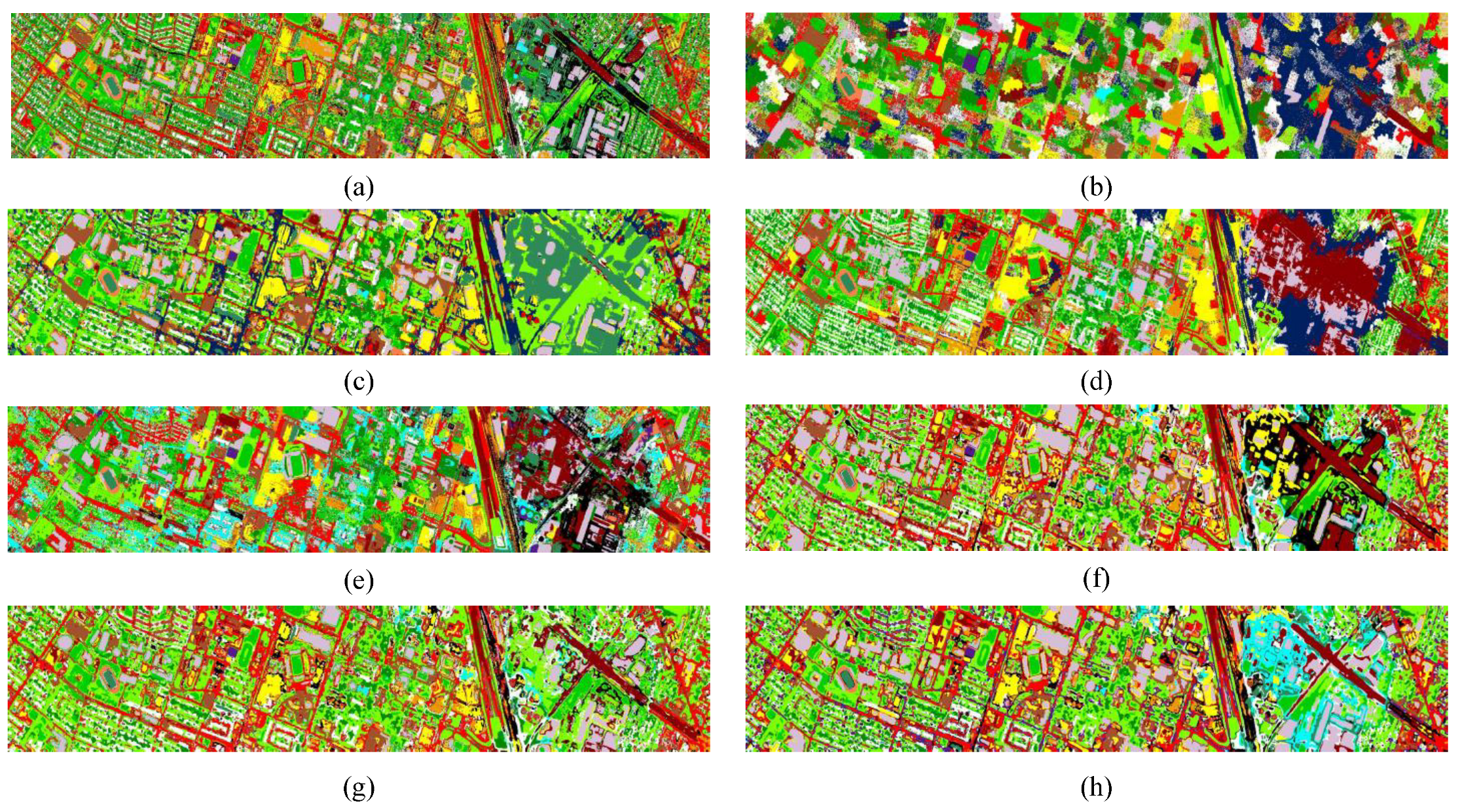
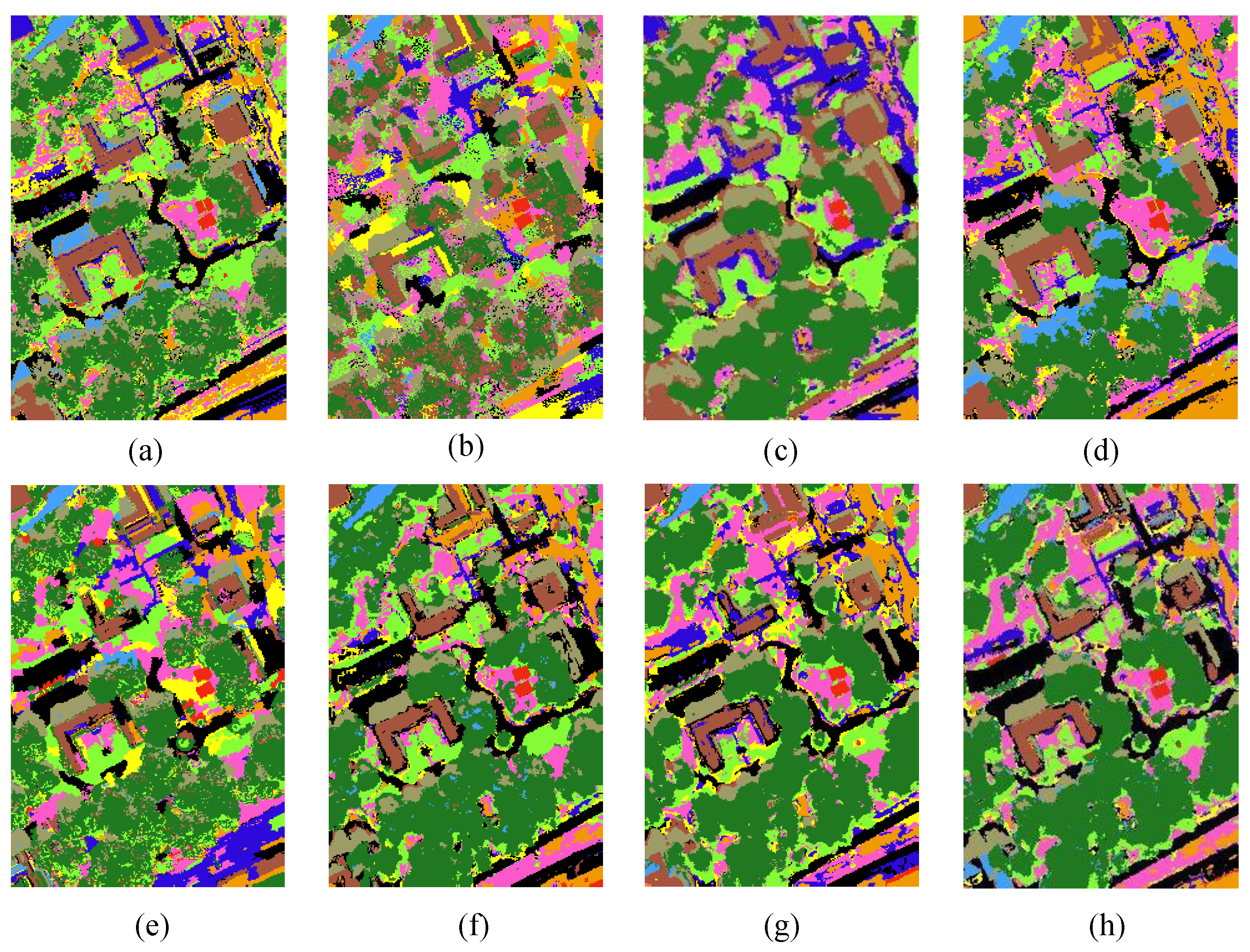
4.7. Comparisons with Other Approaches

A series of experimental verifications are conducted on the Houston and MUUFL Gulfport dataset to verify the effectiveness of the proposed OSGT method. The proposed OSGT method is compared with seven other methods. The specific details of the comparison methods are as follows:
  • SVM:The SVM classifier is applied to stacked HSI and LiDAR data, i.e., H.
  • SuperPCA: The SVM classifier is applied to H.
  • CNN: convolutional neural network [51] for HSI and LiDAR data.
  • ERS: SVM classifier is applied to H, and ERS guides the first three PCs to use the spatial mean strategy based on Gaussian density.
  • NG-OSGT: SVM directly classifies the fusion image obtained by the proposed OSGT method.
  • BG-OSGT: Fusion image band grouping cooperation.
  • MOSGT: Multi-branch decision fusion of the first three PCs and LiDAR data.
Specifically, the SVM parameters are set through five layers of cross-validation, and the parameters of SuperPCA and CNN in the comparison method are the default parameters in the corresponding paper.
The first experiment is conducted on the Houston dataset. Table 1 illustrates the number of training samples and testing samples. The classification performance obtained by different methods is shown in Table 3, and the top results for each class are highlighted in bold typeface. The visual classification maps associated with the corresponding OA of different methods are depicted in Figure 16. As shown in Table 3, SVM just considers the spectral information, so the value of OA is only 78.80%. The problem of cascaded data that does not consider data heterogeneity is most evident in SuperPCA. The heterogeneity of data increases the prominence of the implicit irrelevance pixels within the superpixel, limiting classification performance. Moreover, ERS alleviates the problem of implicit irrelevance using the spatial mean strategy based on Gaussian density. However, the heterogeneity of multi-source data is still the most important influencing factor. The deep learning method represented by CNN has poor algorithm performance under small-sample conditions. NG-OSGT does not illustrate excellent classification accuracy because the fusion result has only one band, and the rich spectral information of HSI is lost. Our purpose is to supplement HSI information with the elevation attribute of LiDAR data as an auxiliary item, rather than abandon the spatial-spectral features of HSI. Consequently, OSGT, BG-OSGT, and MOSGT improve the accuracy of the classifier for ground objects identification.
The second experiment is conducted on the MUUFL Gulfport dataset. Similarly, to further analyze the classification performance of the proposed OSGT method, 10 training samples of each class are randomly selected. The quantitative metrics and classification maps of the compared methods are depicted in Table 4 and Figure 17. When only several training samples are taken for per class, the proposed MOSGT outperforms other comparison methods in terms of visual quality and objective measurement. This demonstrated that the effectiveness of the proposed method in the classification task of HSI and LiDAR data.

4.8. Computational Complexity

Table 5 reports the computational time (in seconds) of each component of the proposed OSGT method. The experiments are performed using MATLAB on a computer with a 2.2 GHz CPU and 8 GB of memory. The training size is 10 per class for Houston and MUUFl Gulfport data sets. As presented in Table 5, the main computational cost of the proposed OSGT method is caused by guided filtering operation. The primary reason is that each band of HSI is the operation object of guided filtering. To solve time-consumption problem, we will study how to use graphics processing units (GPUs) to accelerate our algorithm in future developments.

5. Conclusions

In this paper, a OSGT method is proposed for HSI and LiDAR data classification. Specifically, we define homogeneous region fusion between PCs and LiDAR data as a mathematical optimization problem and introduce the gradient transfer model to fuse spectral and DSM information from various superpixel blocks for the first time. Besides, A l 1 total variation minimization is designed to fuse information between the PC and DSM within each superpixel block to accurately describe the observed details. Experimental results on two real datasets indicated that the proposed methods outperforms the considered baseline methods when there are only ten samples per class for training. In the future, injecting the DSM information of LiDAR data into the classification task of HSI by effectively designing a deep convolutional network is a research direction that we focus on.

Author Contributions

B.T., Y.Z. and C.Z. provided algorithmic ideas for this study, designed experiments and wrote the manuscript. S.C. and A.P. participated in the analysis and evaluation of this work. All authors contributed significantly and participated sufficiently to take responsibility for this research study. All authors have read and agreed to the published version of the manuscript.

Funding

This work was supported in part by the National Natural Science Foundation of China under Grant 61977022, in part by the Science Foundation for Distinguished Young Scholars of Hunan Province under Grant 2020JJ2017, in part by the Key Research and Development Program of Hunan Province under Grant 2019SK2012, in part by the Foundation of Department of Water Resources of Hunan Province under XSKJ2021000-12 and XSKJ2021000-13, in part by the Natural Science Foundation of Hunan Province under Grant 2020JJ4340, and 2021JJ40226, and in part by the Foundation of Education Bureau of Hunan Province under Grant 19A200, 20B257, 20B266, 21B0595 and 21B0590. This work was supported in part by the Open Fund of Education Department of Hunan Province under Grant 20K062. This work was also supported by Junta de Extremadura under Grant GR18060, and by Spanish Ministerio de Ciencia e Innovación through project PID2019-110315RB-I00 (APRISA).

Data Availability Statement

Houston Dataset can be obtained from [9], and MUUFL Gulfport Dataset was obtained from [45,46]. The data generated and analyzed in this study are available on request from the corresponding authors. The data not made public due to follow-up work requirements.

Conflicts of Interest

The authors declare that there is no conflict of interest regarding the publication of this article.

References

  1. Zhou, C.; Tu, B.; Li, N.; He, W.; Plaza, A. Structure-Aware Multikernel Learning for Hyperspectral Image Classification. IEEE J. Sel. Top. Appl. Earth Obs. Remote Sens. 2021, 14, 9837–9854. [Google Scholar] [CrossRef]
  2. AL-Alimi, D.; Al-qaness, M.; Cai, Z.; Dahou, A.; Shao, Y.; Issaka, S. Meta-Learner Hybrid Models to Classify Hyperspectral Images. Remote Sens. 2022, 14, 1038. [Google Scholar] [CrossRef]
  3. Xi, J.; Ersoy, O.; Fang, J.; Cong, M.; Wu, T.; Zhao, C.; Li, Z. Wide Sliding Window and Subsampling Network for Hyperspectral Image Classification. Remote Sens. 2021, 13, 1290. [Google Scholar] [CrossRef]
  4. Wu, L.; Gao, Z.; Liu, Y.; Yu, H. Study of uncertainties of hyperspectral image based on Fourier waveform analysis. In Proceedings of the IGARSS 2004, Anchorage, AK, USA, 20–24 September 2004; Volume 5, pp. 3279–3282. [Google Scholar]
  5. Zhou, C.; Tu, B.; Ren, Q.; Chen, S. Spatial Peak-Aware Collaborative Representation for Hyperspectral Imagery Classification. IEEE Geosci. Remote Sens. Lett. 2022, 19, 1–5. [Google Scholar] [CrossRef]
  6. Gao, R.; Li, M.; Yang, S.; Cho, K. Reflective Noise Filtering of Large-Scale Point Cloud Using Transformer. Remote Sens. 2022, 14, 577. [Google Scholar] [CrossRef]
  7. Ojogbane, S.; Mansor, S.; Kalantar, B.; Khuzaimah, Z.; Shafri, H.; Ueda, N. Automated Building Detection from Airborne LiDAR and Very High-Resolution Aerial Imagery with Deep Neural Network. Remote Sens. 2021, 13, 4803. [Google Scholar] [CrossRef]
  8. Gu, Y.; Wang, Q. Discriminative Graph-Based Fusion of HSI and LiDAR Data for Urban Area Classification. IEEE Geosci. Remote Sens. Lett. 2017, 14, 906–910. [Google Scholar] [CrossRef]
  9. Debes, C.; Merentitis, A.; Heremans, R.; Hahn, J.; Frangiadakis, N.; Kasteren, T.; Liao, W.; Bellens, R.; Pižurica, A.; Gautama, S. Hyperspectral and LiDAR Data Fusion: Outcome of the 2013 GRSS Data Fusion Contest. IEEE J. Sel. Top. Appl. Earth Observ. Remote Sens. 2014, 7, 2405–2418. [Google Scholar] [CrossRef]
  10. Saunders, C.; Stitson, M.; Weston, J.; Holloway, R.; Bottou, L.; Scholkopf, B.; Smola, A. Support Vector Machine. Comput. Sci. 2002, 1, 1–28. [Google Scholar]
  11. Chen, Y. Multiple Kernel Feature Line Embedding for Hyperspectral Image Classification. Remote Sens. 2019, 11, 2892. [Google Scholar] [CrossRef] [Green Version]
  12. Li, J.; Bioucas-Dias, J.; Plaza, A. Spectral–Spatial Hyperspectral Image Segmentation Using Subspace Multinomial Logistic Regression and Markov Random Fields. IEEE Trans. Geosci. Remote Sens. 2012, 50, 809–823. [Google Scholar] [CrossRef]
  13. Haut, J.; Paoletti, M. Cloud Implementation of Multinomial Logistic Regression for UAV Hyperspectral Images. IEEE J. Miniat. Air Space Syst. 2020, 1, 163–171. [Google Scholar] [CrossRef]
  14. Zhong, Y.; Zhang, L. An Adaptive Artificial Immune Network for Supervised Classification of Multi-/Hyperspectral Remote Sensing Imagery. IEEE Trans. Geosci. Remote Sens. 2012, 50, 894–909. [Google Scholar] [CrossRef]
  15. Zhang, X.; Shang, S.; Tang, X.; Feng, J.; Jiao, L. Spectral Partitioning Residual Network with Spatial Attention Mechanism for Hyperspectral Image Classification. IEEE Trans. Geosci. Remote Sens. 2022, 60, 5507714. [Google Scholar] [CrossRef]
  16. Cui, Y.; Xia, J.; Wang, Z.; Gao, S.; Wang, L. Lightweight Spectral-Spatial Attention Network for Hyperspectral Image Classification. IEEE Trans. Geosci. Remote Sens. 2022, 60, 5510114. [Google Scholar] [CrossRef]
  17. Meng, Z.; Zhao, F.; Liang, M. SS-MLP: A Novel Spectral-Spatial MLP Architecture for Hyperspectral Image Classification. Remote Sens. 2021, 13, 4060. [Google Scholar] [CrossRef]
  18. Wang, J.; Huang, R.; Guo, S.; Li, L.; Pei, Z.; Liu, B. HyperLiteNet: Extremely Lightweight Non-Deep Parallel Network for Hyperspectral Image Classification. Remote Sens. 2022, 14, 866. [Google Scholar] [CrossRef]
  19. Fang, L.; Wang, C.; Li, S.; Benediktsson, J. Hyperspectral Image Classification via Multiple-Feature-Based Adaptive Sparse Representation. IEEE Trans. Instrum. Meas. 2017, 66, 1646–1657. [Google Scholar] [CrossRef]
  20. Ding, Y.; Guo, Y.; Chong, Y.; Pan, S.; Feng, J. Global Consistent Graph Convolutional Network for Hyperspectral Image Classification. IEEE Trans. Instrum. Meas. 2021, 70, 1–16. [Google Scholar] [CrossRef]
  21. Zhang, Z.; Liu, D.; Gao, D.; Shi, G. S3Net: Spectral-Spatial-Semantic Network for Hyperspectral Image Classification with the Multiway Attention Mechanism. IEEE Trans. Geosci. Remote Sens. 2022, 60, 1–17. [Google Scholar]
  22. Chen, Y.; Xu, L.; Fang, Y.; Peng, J.; Yang, W.; Wong, A.; Clausi, D. Unsupervised Bayesian Subpixel Mapping of Hyperspectral Imagery Based on Band-Weighted Discrete Spectral Mixture Model and Markov Random Field. IEEE Geosci. Remote Sens. Lett. 2021, 18, 162–166. [Google Scholar] [CrossRef]
  23. Andrejchenko, V.; Liao, W.; Philips, W.; Scheunders, P. Decision Fusion Framework for Hyperspectral Image Classification Based on Markov and Conditional Random Fields. Remote Sens. 2019, 11, 624. [Google Scholar] [CrossRef] [Green Version]
  24. Yu, H.; Shang, X.; Song, M.; Hu, J.; Jiao, T.; Guo, Q.; Zhang, B. Union of Class-Dependent Collaborative Representation Based on Maximum Margin Projection for Hyperspectral Imagery Classification. IEEE J. Sel. Top. Appl. Earth Obs. Remote Sens. 2021, 14, 553–566. [Google Scholar] [CrossRef]
  25. Su, H.; Yu, Y.; Du, Q.; Du, P. Ensemble Learning for Hyperspectral Image Classification Using Tangent Collaborative Representation. IEEE Trans. Geosci. Remote Sens. 2020, 58, 3778–3790. [Google Scholar] [CrossRef]
  26. Zhong, S.; Chang, C.; Zhang, Y. Iterative Edge Preserving Filtering Approach to Hyperspectral Image Classification. IEEE Geosci. Remote Sens. Lett. 2019, 16, 90–94. [Google Scholar] [CrossRef]
  27. Wei, Y.; Zhou, Y. Spatial-Aware Network for Hyperspectral Image Classification. Remote Sens. 2021, 13, 3232. [Google Scholar] [CrossRef]
  28. Khodadadzadeh, M.; Li, J.; Prasad, S.; Plaza, A. Fusion of Hyperspectral and LiDAR Remote Sensing Data Using Multiple Feature Learning. IEEE J. Sel. Topics Appl. Earth Observ. Remote Sens. 2015, 8, 2971–2983. [Google Scholar] [CrossRef]
  29. Wang, P.; Wang, Y.; Zhang, L.; Ni, K. Subpixel Mapping Based on Multisource Remote Sensing Fusion Data for Land-Cover Classes. IEEE Geosci. Remote Sens. Lett. 2022, 19, 1–5. [Google Scholar] [CrossRef]
  30. Zhao, X.; Tao, R.; Li, W.; Philips, W.; Liao, W. Fractional Gabor Convolutional Network for Multisource Remote Sensing Data Classification. IEEE Trans. Geosci. Remote Sens. 2022, 60, 1–18. [Google Scholar] [CrossRef]
  31. Jahan, F.; Zhou, J.; Awrangjeb, M.; Gao, Y. Inverse Coefficient of Variation Feature and Multilevel Fusion Technique for Hyperspectral and LiDAR Data Classification. IEEE J. Sel. Topics Appl. Earth Observ. Remote Sens. 2020, 13, 367–381. [Google Scholar] [CrossRef] [Green Version]
  32. Chen, Y.; Li, C.; Ghamisi, P.; Jia, X.; Gu, Y. Deep Fusion of Remote Sensing Data for Accurate Classification. IEEE Geosci. Remote Sens. Lett. 2017, 14, 1253–1257. [Google Scholar] [CrossRef]
  33. Huang, Q.; Miao, Z.; Zhou, S.; Chang, C.; Li, X. Dense Prediction and Local Fusion of Superpixels: A Framework for Breast Anatomy Segmentation in Ultrasound Image With Scarce Data. IEEE Trans. Instrum. Meas. 2021, 70, 1–8. [Google Scholar] [CrossRef]
  34. Jia, S.; Zhan, Z.; Zhang, M.; Xu, M.; Huang, Q.; Zhou, J.; Jia, X. Multiple Feature-Based Superpixel-Level Decision Fusion for Hyperspectral and LiDAR Data Classification. IEEE Trans. Geosci. Remote Sens. 2021, 59, 1437–1452. [Google Scholar] [CrossRef]
  35. Zhao, W.; Jiao, L.; Ma, W.; Zhao, J.; Zhao, J.; Liu, H.; Cao, X.; Yang, S. Superpixel-Based Multiple Local CNN for Panchromatic and Multispectral Image Classification. IEEE Trans. Geosci. Remote Sens. 2017, 55, 4141–4156. [Google Scholar] [CrossRef]
  36. Jiang, J.; Ma, J.; Chen, C.; Wang, Z.; Cai, Z.; Wang, L. SuperPCA: A Superpixelwise PCA Approach for Unsupervised Feature Extraction of Hyperspectral Imagery. IEEE Trans. Geosci. Remote Sens. 2018, 56, 4581–4593. [Google Scholar] [CrossRef] [Green Version]
  37. Zhang, X.; Jiang, X.; Jiang, J.; Zhang, Y.; Liu, X.; Cai, Z. Spectral-Spatial and Superpixelwise PCA for Unsupervised Feature Extraction of Hyperspectral Imagery. IEEE Trans. Geosci. Remote Sens. 2022, 60, 1–10. [Google Scholar] [CrossRef]
  38. Liu, M.; Tuzel, O.; Ramalingam, S.; Chellappa, R. Entropy-Rate Clustering: Cluster Analysis via Maximizing a Submodular Function Subject to a Matroid Constraint. IEEE Trans. Pattern Anal. Mach. Intell. 2014, 36, 99–112. [Google Scholar] [CrossRef]
  39. He, K.; Jian, S.; Tang, X. Guided image filtering. In Proceedings of the 11th European Conference on Computer Vision, Heraklion, Greece, 5–11 September 2010; Springer: Berlin/Heidelberg, Germany, 2010; pp. 1–14. [Google Scholar]
  40. Wu, L.; Jong, C. A High-Throughput VLSI Architecture for Real-Time Full-HD Gradient Guided Image Filter. IEEE Trans. Circuits Syst. Video Technol. 2019, 29, 1868–1877. [Google Scholar] [CrossRef]
  41. Yang, Y.; Wan, W.; Huang, S.; Yuan, F.; Yang, S.; Que, Y. Remote Sensing Image Fusion Based on Adaptive IHS and Multiscale Guided Filter. IEEE Access 2016, 4, 4573–4582. [Google Scholar] [CrossRef]
  42. Fang, J.; Hu, S.; Ma, X. SAR image de-noising via grouping-based PCA and guided filter. IEEE J. Syst. Eng. Electron. 2021, 32, 81–91. [Google Scholar]
  43. Draper, N. Applied regression analysis. Technometrics 1998, 9, 182–183. [Google Scholar]
  44. Chan, T.; Esedoglu, S. Aspects of total variation regularized L1 function approximation. SIAM J. Appl. Math. 2005, 65, 1817–1837. [Google Scholar] [CrossRef] [Green Version]
  45. Gader, P.; Zare, A.; Close, R.; Aitken, J.; Tuell, G. Muufl Gulfport Hyperspectral and Lidar Airborne Data Set; University of Florida: Gainesville, FL, USA, 2013. [Google Scholar]
  46. Du, X.; Zare, A. Technical Report: Scene Label Ground Truth Map for Muufl Gulfport Data Set; University of Florida: Gainesville, FL, USA, 2017. [Google Scholar]
  47. Kang, X.; Li, C.; Li, S.; Lin, H. Classification of Hyperspectral Images by Gabor Filtering Based Deep Network. IEEE J. Sel. Top. Appl. Earth Observ. Remote Sens. 2018, 11, 1166–1178. [Google Scholar] [CrossRef]
  48. Karam, C.; Hirakawa, K. Monte-Carlo Acceleration of Bilateral Filter and Non-Local Means. IEEE Trans. Image Process. 2018, 27, 1462–1474. [Google Scholar] [CrossRef] [PubMed]
  49. Kang, X.; Li, S.; Benediktsson, J. Feature Extraction of Hyperspectral Images with Image Fusion and Recursive Filtering. IEEE Trans. Geosci. Remote Sens. 2014, 52, 3742–3752. [Google Scholar] [CrossRef]
  50. Chen, Z.; Jiang, J.; Zhou, C.; Fu, S.; Cai, Z. SuperBF: Superpixel-Based Bilateral Filtering Algorithm and Its Application in Feature Extraction of Hyperspectral Images. IEEE Access 2019, 7, 147796–147807. [Google Scholar] [CrossRef]
  51. Xu, X.; Li, W.; Ran, Q.; Du, Q.; Gao, L.; Zhang, B. Multisource Remote Sensing Data Classification Based on Convolutional Neural Network. IEEE Trans. Geosci. Remote Sens. 2018, 56, 937–949. [Google Scholar] [CrossRef]
Figure 1. Schematic illustration of image fusion. (a) The first PC of the Houston dataset. (b) LiDAR data. (c) The fusion result of stacking method. (d) OSGT-based fusion image.
Remotesensing 14 01814 g001
Figure 2. Outline of the proposed OSGT method for hyperspectral and LiDAR data classification.
Remotesensing 14 01814 g002
Figure 3. A local spatial mean regularization strategy based on Gaussian density.
Remotesensing 14 01814 g003
Figure 4. Spectral characteristics (a) before and (b) after Guided filtering. We take class Railway in Houston dataset for example.
Remotesensing 14 01814 g004
Figure 5. The first 10 principal component images of the MUUFL Gulfport dataset are based on PCA algorithm.
Remotesensing 14 01814 g005
Figure 6. Visualization of the Houston data. (a) Pseudo-color image for the hyperspectral data. (b) Grayscale image for the LiDAR data. (c) Ground truth.
Remotesensing 14 01814 g006
Figure 7. Visualization of the MUUFL Gulfport. (a) Pseudo-color image for the hyperspectral data. (b) Grayscale image for the LiDAR data. (c) Ground truth.
Remotesensing 14 01814 g007
Figure 8. Effect of the number of superpixels on the overall classification accuracy (%) of OSGT method for Houston (a–c) and MUUFL Gulfport (d–f) datasets. Different numbers of training samples determine the results of each column. Specifically, the first to third columns are the classification accuracy when the number of training samples is 5, 10, and 15 per class, respectively.
Remotesensing 14 01814 g008
Figure 9. Effect of r and ξ to the performance of classification for different datasets. (a) Houston dataset. (b) MUUFL Gulfport dataset.
Remotesensing 14 01814 g009
Figure 10. Visualized fusion results and quantitative indicator under different free parameters for Houston dataset. (a) The first PC image, (b) LiDAR data, (ch) Fusion result when λ = 0.1 , 0.5 , 1 , 5 , 10 , 50 , respectively. (i) Overall Accuracy.
Remotesensing 14 01814 g010
Figure 11. Visualized fusion results and quantitative indicator under different free parameters for MUUFL Gulfport dataset. (a) The first PC image, (b) LiDAR data, (ch) Fusion result when λ = 0.1 , 0.5 , 1 , 5 , 10 , 50 , respectively. (i) Overall Accuracy.
Remotesensing 14 01814 g011
Figure 12. Analyze the auxiliary effect of LiDAR data on HSI for (a) Houston dataset and (b) MUUFL Gulfport.
Remotesensing 14 01814 g012
Figure 13. Classification accuracy (i.e., OA, AA, and Kappa) of the proposed OSGT method using different filtering methods. (a) OA, (b) AA and (c) Kappa for Houston, (d) OA, (e) AA and (f) Kappa for MUUFL Gulfport dataset.
Remotesensing 14 01814 g013
Figure 14. Visualization results of the proposed OSGT method with different filtering methods (i.e., (a) Gabor filtering (GaF), (b) mean filtering (MF), (c) recursive filtering (RF), (d) bilateral filtering (BF) and (e) guided filtering (GuF).) and (f) pseudo-color image on the Houston dataset.
Remotesensing 14 01814 g014
Figure 15. Visualization results of the proposed OSGT method with different filtering methods (i.e., (a) Gabor filtering (GaF), (b) mean filtering (MF), (c) recursive filtering (RF), (d) bilateral filtering (BF) and (e) guided filtering (GuF).) and (f) pseudo-color image on the MUUFL Gulfport dataset.
Remotesensing 14 01814 g015
Figure 16. Houston dataset: classification maps obtained by: (a) SVM, (b) SuperPCA, (c) CNN, (d) ERS, (e) NG-OSGT, (f) OSGT, (g) BG-OSGT and (h) MOSGT when the number of training samples is ten per class.
Remotesensing 14 01814 g016
Figure 17. MUUFL Guflport: classification maps obtained by:(a) SVM, (b) SuperPCA, (c) CNN, (d) ERS, (e) NG-OSGT, (f) OSGT, (g) BG-OSGT and (h) MOSGT when the number of training samples is ten per class.
Remotesensing 14 01814 g017
Table 1. Different numbers of training and testing samples for fifteen classes in the Houston and eleven classes in the MUUFL Gulfport.
HoustonMUUFL Gulfport
ClassLand-Cover TypeTrainingTestClassLand-Cover TypeTrainingTest
C1Healthy grass101241C1Trees1023,236
C2Stressed grass101244C2Mostly Grass104260
C3Synthetic grass10687C3Mixed Ground106872
C4Tree101234C4Dirt and Sand101816
C5Soil101232C5Roads106677
C6Water10315C6Water10456
C7Residential101258C7Building Shadows102223
C8Commercial101234C8Buildings106230
C9Road101242C9Sidewalks101375
C10Highway101217C10Yellow Curbs10173
C11Railway101225C11Cloth Panels10259
C12Parking lot 1101223
C13Parking lot 210459
C14Tennis court10418
C15Running track10650
Total 15014,879 11053,577
Table 2. Classification accuracy (in %) of Houston and MUUFL Guflport with no superpixels, global feature fusion and local feature fusion methods.
Houston Data Set
metricsNSLNSPPCL-GTFP C 3 L-GTFOSGT
OA(%)78.1276.3979.8379.5581.02
AA(%)78.576.6680.6680.2581.09
Kappa0.760.750.780.780.79
MUUFL Gulfport Data Set
metricsNSLNSPPCL-GTFP C 3 L-GTFOSGT
OA(%)68.6868.8570.8271.1272.59
AA(%)52.7156.5856.0656.5468.69
Kappa0.610.610.630.640.68
Table 3. Classification performance using SVM, SuperPCA, CNN, ERS, NG-OSGT, OSGT, BG-OSGT and MOSGT for Houston dataset with ten labeled samples per class as training set.
ClassSVMSuperPCACNNERSNG-OSGTOSGTBG-OSGTMOSGT
C193.1254.1279.3677.9672.9493.6890.7390.03
C282.3147.1993.4450.5168.2587.0887.9090.29
C368.6598.1199.8994.7680.1389.9483.7587.71
C482.4731.9048.3445.7375.6092.1497.5694.61
C592.0177.0981.0578.1769.0690.8590.2286.38
C694.4883.5262.2550.0058.9582.8090.9572.61
C767.2736.4177.4678.3869.1478.8378.2176.59
C878.9733.4852.9370.8758.6782.1588.8279.47
C983.0337.1161.1876.7370.9376.4473.0879.56
C1063.6862.5039.0263.8954.6270.5483.6081.62
C1159.1676.8654.8060.6562.0470.2376.7580.40
C1257.7250.9383.7870.1660.7076.7888.3684.13
C1340.7858.000.9859.1647.6255.2570.4471.44
C1469.95100.0090.3190.2885.9779.9797.2382.57
C1598.6381.2388.3898.1976.6598.0498.6498.05
OA75.3953.5264.6868.7166.3781.1885.3983.38
AA77.3849.0964.8171.3467.4281.5986.4083.36
Kappa0.730.630.620.660.640.800.840.82
Table 4. Classification performance using SVM, SuperPCA, CNN, ERS, NG-OSGT, OSGT, BG-OSGT and MOSGT for MUUFL Gulfpor dataset with ten labeled samples per class as training set.
ClassSVMSuperPCACNNERSNG-OSGTOSGTBG-OSGTMOSGT
C196.9440.3462.3796.7293.3896.9594.3594.54
C255.1632.5590.2150.3650.0347.3052.8751.27
C365.4227.8333.7952.9366.2768.7170.0274.71
C455.0239.9460.2456.0338.1354.8455.3957.93
C587.2428.5560.1569.9068.4777.6373.1278.49
C653.7086.144.4132.1328.4140.3353.7238.31
C739.0177.2278.6952.8241.4651.2947.4856.20
C883.1440.8359.5596.0460.7083.3688.6490.41
C930.9136.6723.4834.2812.8325.6441.1944.60
C1013.0432.204.341.361.306.859.968.73
C1154.3185.5658.1999.5832.4656.2186.5483.57
OA70.5938.7159.2270.9959.4872.6774.5775.63
AA57.6227.4548.6758.3744.8664.6761.2161.71
Kappa0.640.480.500.640.50.560.670.69
Table 5. Calculation time (in seconds) for different components and guiding images.
Data SetDifferent ComponentsDifferent Guide Images
ERSOSGTGFG-PCAG-LiDAR
Houston8.690.1933.4732.9432.76
MUUFL Gulfport0.600.090.940.950.93
Publisher’s Note: MDPI stays neutral with regard to jurisdictional claims in published maps and institutional affiliations.

