Surround-Net: A Multi-Branch Arbitrary-Oriented Detector for Remote Sensing

Abstract

With the development of oriented object detection technology, especially in the area of remote sensing, significant progress has been made, and multiple excellent detection architectures have emerged. Oriented detection architectures can be broadly divided into five-parameter systems and eight-parameter systems that encounter the periodicity problem of angle regression and the discontinuous problem of vertex regression during training, respectively. Therefore, we propose a new multi-branch anchor-free one-stage model that can effectively alleviate the corner case when representing rotating objects, called Surround-Net. The creative contribution submitted in this paper mainly includes three aspects. Firstly, a multi-branch strategy is adopted to make the detector choose the best regression path adaptively for the discontinuity problem. Secondly, to address the inconsistency between classification and quality estimation (location), a modified high-dimensional Focal Loss and a new Surround IoU Loss are proposed to enhance the unity ability of the features. Thirdly, in the refined process after backbone feature extraction, a center vertex attention mechanism is adopted to deal with the environmental noise introduced in the remote sensing images. This type of auxiliary module is able to focus the model’s attention on the boundary of the bounding box. Finally, extensive experiments were carried out on the DOTA dataset, and the results demonstrate that Surround-Net can solve regression boundary problems and can achieve a more competitive performance (e.g., 75.875 mAP) than other anchor-free one-stage detectors with higher speeds.

1. Introduction

As one of the most important basic tasks in computer vision, object detection has attracted the attention of many researchers and has been studied extensively. The main goal of this task is to find the location of an object in an image and label the category that it belongs to. It can be used as a key component in many downstream tasks.

With the rise of deep learning technology, object detection has developed quickly. Architectures can be divided into two-stage and one-stage architectures depending on the processing stage [1]. For example, the R-CNN family [2,3,4] and its improvements [5,6,7] follow the “coarse-to-fine” pipeline. On the contrary, one-stage architectures, such as the YOLO family [8,9,10,11], SSD [12], and RetinaNet [13], are able to complete detection tasks in one step. Although they have a good running speed, their accuracy is not high compared to two-stage architectures. In addition, models can also be divided into the anchor-base category [2,3,4,5,6,7,9,10,11,12,13,14], which requires multiple anchors of different sizes and proportions, and the anchor-free category [15,16,17,18], in which the object is represented as a point. The former has higher accuracy, while the latter is easier to train and adjust.

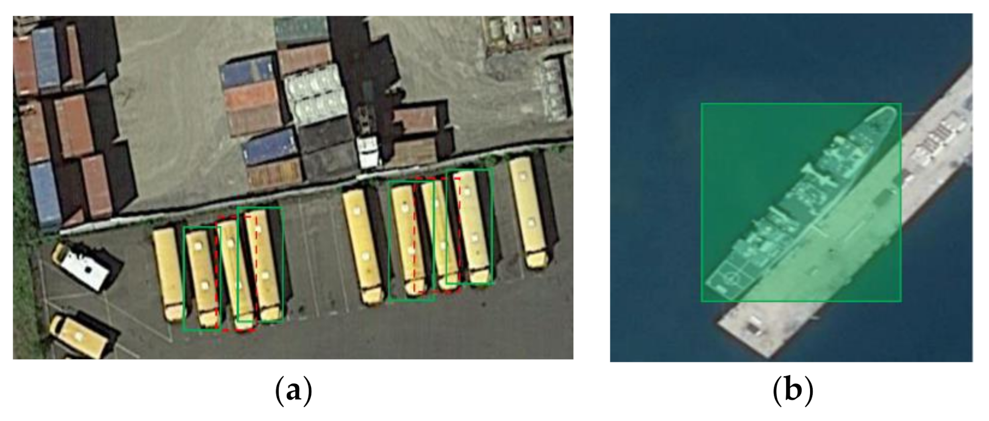
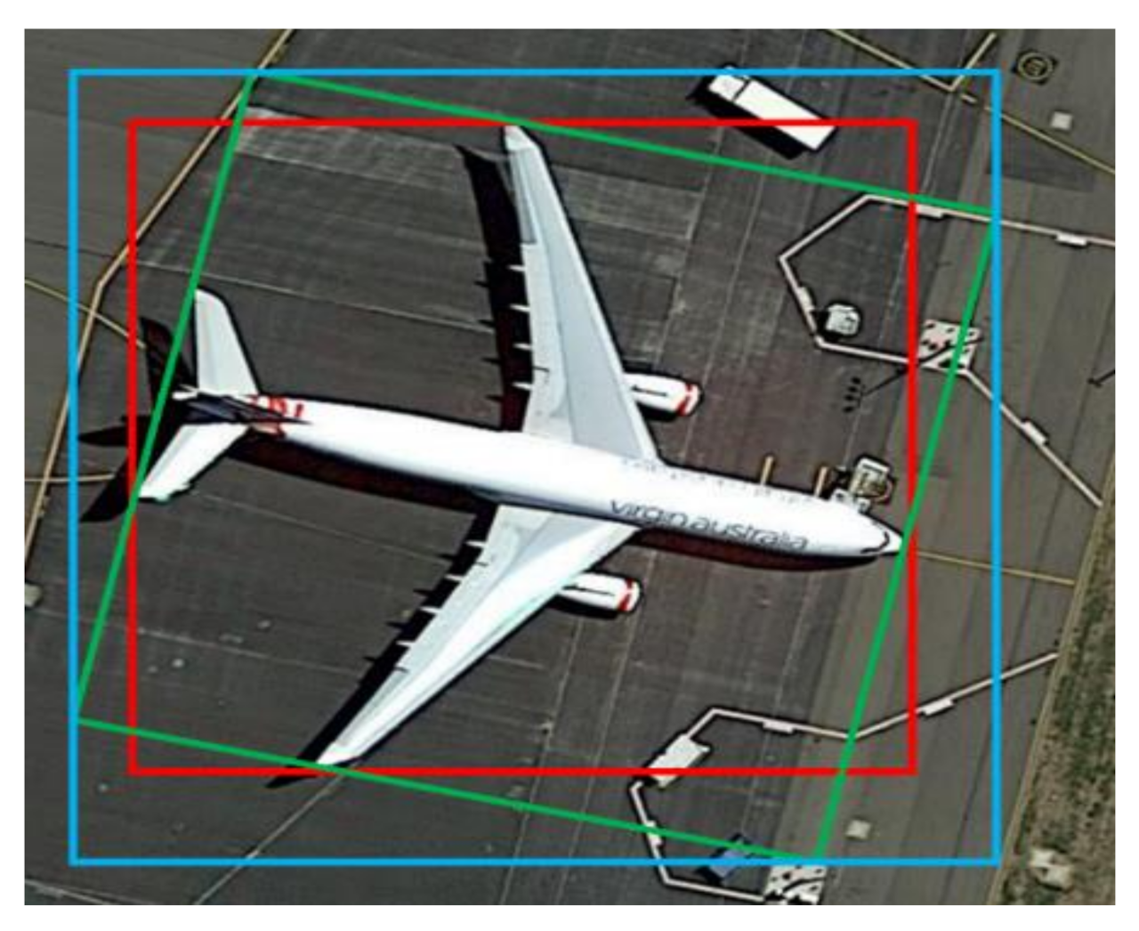
Recently, object detection tasks in arbitrary directions have received more and more attention. In the field of remote sensing detection, oriented detection can not only identify densely packed objects but also ones with a huge aspect ratio. Figure 1 shows the limitations of horizontal object detection.

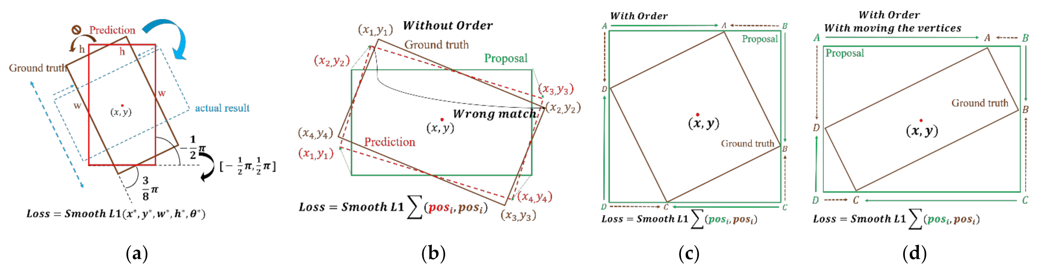
Most oriented object detectors are adapted from horizontal object detectors, and they can be broadly divided into five-parameter models [19,20,21,22,23,24,25] and eight-parameter models [26,27,28,29,30]. The five-parameter models add an angle parameter ($x,y,w,h,\theta$) and achieve great success. However, these detectors inevitably suffer from the angle boundary problem during training. As shown in Figure 2a, assuming that the center coordinates of the two boxes coincide (without loss of generality), the red box (Prediction, −1/2π) needs to match the brown box (Ground-truth, 3/8π), something that can be achieved by adjusting the angle and size. An ideal regression method rotates the prediction box counterclockwise without resizing it. However, due to the boundary characteristics of the angle, the prediction box can not achieve its purpose because of the sudden change. Instead, it must rotate 3/8π clockwise and adjust its size simultaneously. SCRDet [25] introduces IoU-Loss to enable the model to find a better regression method, but it cannot eliminate it.

The eight-parameter models were proposed to solve the angle problems that are present in the five-parameter models. They cover the detection task using a point-based method by directly predicting four vertices. However, such a direct method introduces new problems. First, it is necessary to sort the vertices when calculating the regression loss. Otherwise, the almost identical rectangle will still produce a colossal Loss (as shown in Figure 2b); secondly, as described in Figure 2c, the sorted order may still be sub-optimal. In addition to regression, along with a clockwise method (green line), there is an ideal regression method (brown line). RSDet [31,32] proposes comparing the Loss after moving the vertexes one unit clockwise and one unit counterclockwise. However, this approach only solves part of the problem. When faced with the situation shown in Figure 2d, no matter how the adjustments are made, there are still sub-optimal paths (two longer regression paths always exist).

After analyzing the above ranking and regression discontinuity problems, we propose a multi-branch eight-parameter model called Surround-Net. It decomposes the prediction process into multiple branches to take all cases into account in an anchor-free and one-stage way. To improve the model’s consistency during testing and training, a modified multi-branch-aware adaptive Focal Loss function [13] is creatively proposed so that the classification branch selection can be trained simultaneously. A size-adaptive dense prediction module is proposed to alleviate the imbalance between the positive and negative samples. Moreover, to enhance the model’s performance during localization, this work also presents a novel center vertex attention mechanism and a geometric soft constraint. The results further show that Surround-Net can solve the sub-optimal emerge problem present in previous models and can achieve a competitive result (e.g., 75.875 mAP and 74.071 mAP in 12.57 FPS) in an anchor-free one-stage way. Overall, our contributions are as follows:

• A multi-branch anchor-free detector for oriented object detection is proposed and solves the sorting and suboptimal regression problems encountered with eight-parameter models;
• To jointly training branch selection and class prediction, we propose a modified Focal Loss function, and a size-adaptived dense prediction module is adopted to alleviate the imbalance between the positive and negative samples;
• We propose a center vertex attention mechanism to distinguish the environment area and use soft constraints to refine the detection boxes.

2. Materials and Methods

First, we will provide an overview of the content structure. The architecture of our proposed anchor-free one-stage model is introduced in Section 2.1. Section 2.2 elaborates on the multi-branch structure and the adaptive function design for dense predictions as well as on the multi-branch adaptive Focal Loss for joint training. The prediction of the circumscribed rectangle and sliding ratios are discussed in Section 2.3, and the soft constraints for refinement are introduced in that section as well. Finally, we describe how to encode a rotating detection box using all of the predicted values. The center vertex attention mechanism for feature optimization is introduced in Section 2.4.

2.1. Architecture

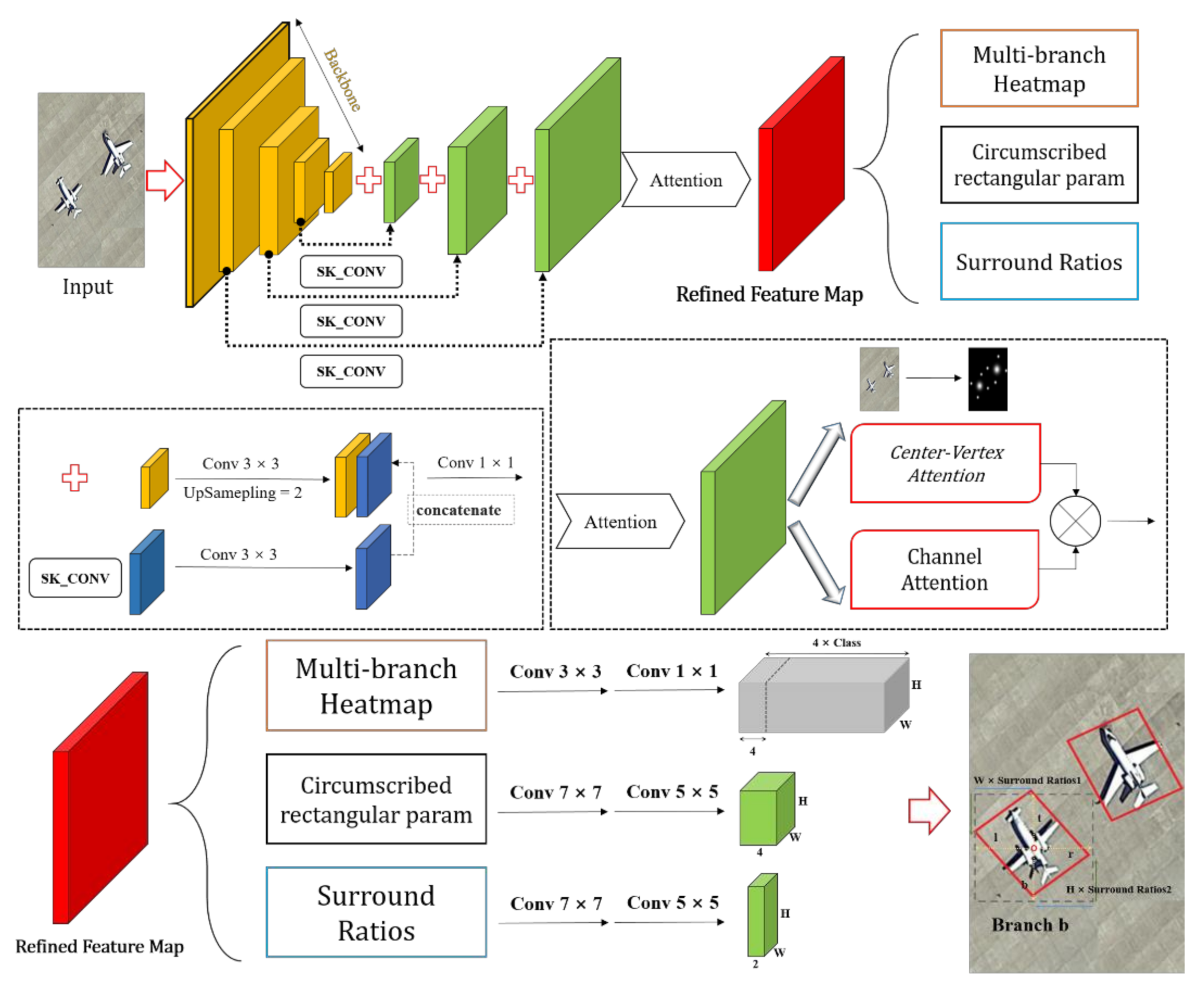
As shown in Figure 3, the whole pipeline can be divided into the following four cascading modules: the feature extraction module, the feature combination module, the feature refine module, and the prediction head module. Initially, we use 1–5 convolutional ResNet-101 (ResNet-152 for better performance) layers and resize the final output feature map to 1/4 of the original input image size. In the up-sampling process, we first use 3 × 3 convolutions to resize the small-scale feature maps with rich semantic information to the same size as the feature maps from the previous levels. At the same time, the concatenate operation is performed on the feature map from a previous level that contains more delicate details via a 3 × 3 convolution layer. After completing one concatenation layer, it is followed by a 1 × 1 convolutional layer to enhance the fusion of the channel elements in the feature map. Before entering the next up-sampling stage, batch normalization [33] and Leaky ReLU [34] were used to normalize the feature map and improve its nonlinear fitting ability. At the tail of the feature combination, an attention module is proposed to refine the feature map. This part will be detailed in Section 2.4. Inspired by TSD [35], we also added additional convolutional layers for each prediction head in a decoupled manner.

There are three detection heads that follow the following refined feature map: the multi-branch selection and classification head, the circumscribed rectangle prediction head, and the sliding ratio prediction head. For the multi-branch selection and classification head, the number of filters is 4 × C, where C is the number of categories and 4 is the number of different branches; for the circumscribed rectangle prediction head, the number is 4, representing the four distances ($l,r,t,b$) from the center point to their corresponding circumscribed rectangle; for the sliding ratio prediction head, the number is 2, representing the two required ratios.

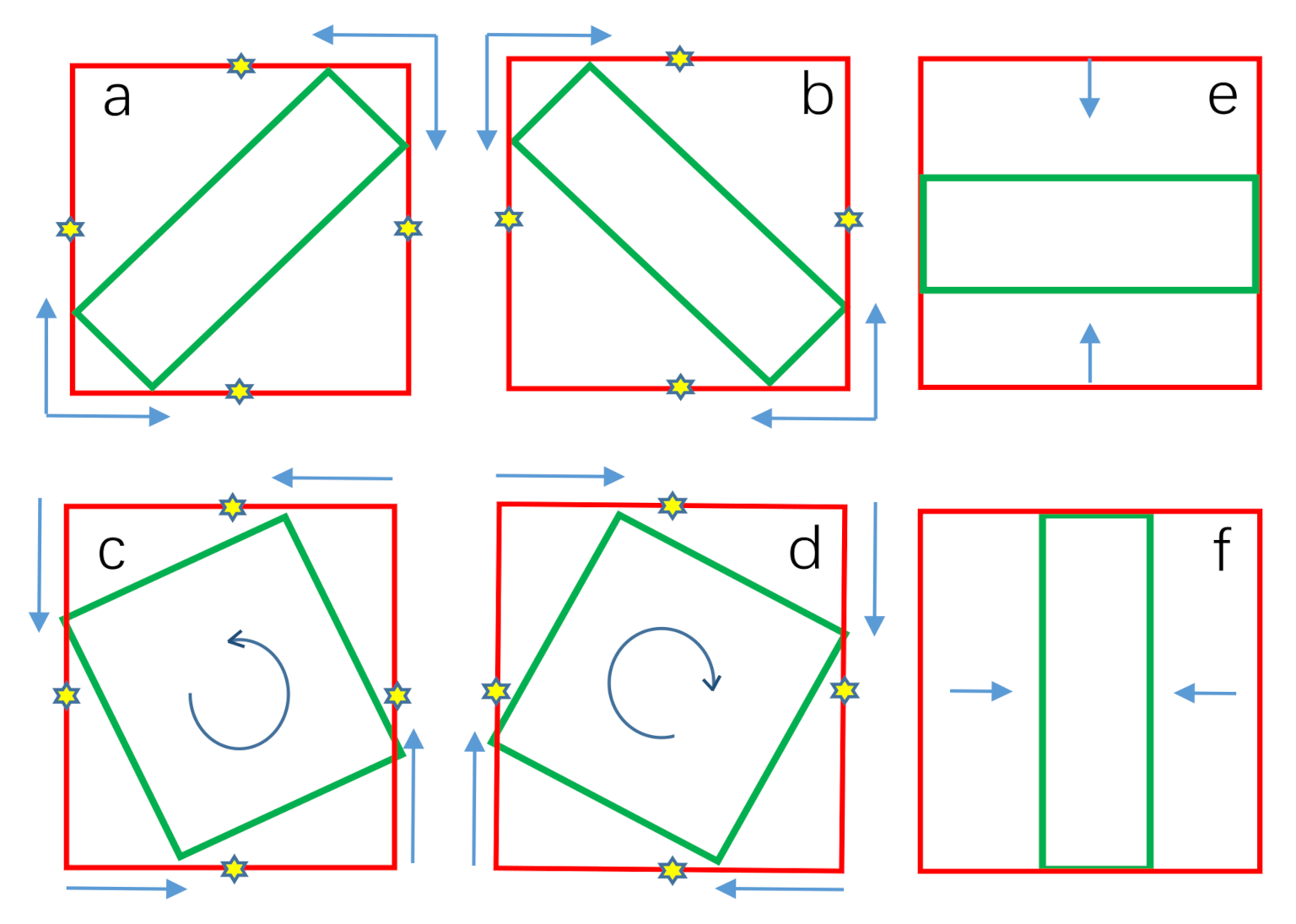
As shown in Figure 4a–d, we divided the rotating bounding boxes obtained from the circumscribed rectangle into four cases corresponding to the multi-branch selection head.

The yellow star represents the midpoint of the boundary of the circumscribed rectangle. According to the coordinates falling on the boundary, the regression process can be divided into the following two cases: Figure 4a–d. In the first case, starting from a vertex of the circumscribed rectangle and sliding in the horizontal and vertical directions, a rotating bounding box can be obtained optimally. In the second case, the sliding vertices can be selected either counterclockwise or clockwise. This once again represents an optimal regression method and achieves the same results as RSDet [31,32]. The cases corresponding to Figure 4e,f can be regarded as the prediction of the horizontal bounding box whose sliding ratios are close to 0. Therefore, using the multi-branch regression method, the suboptimal regression problem shown in Figure 2b–d is solved. Section 2.2 describes how to use multi-branch prediction to find the best regression method in the above four regression branches.

2.2. Potential Points of the Object

According to Figure 3, it can be seen that the output of the multi-branch selection and classification head is a heat map in ${ℝ}^{4\mathrm{C}\times W\times H}$ for an input RGB image in ${ℝ}^{3\times H^{\prime }\times W^{\prime }}$, where $H^{\prime }$ and $W^{\prime }$ are the height and width of the image and $H=H^{\prime }/4$, $W=W^{\prime }/4$. We expanded the prediction channel and replaced the classification score with the PQES (prediction quality estimated score) (this will be explained in detail later) to measure whether the rotated bounding box obtained through the current branch had the highest IoU (Intersection-over-Union) with the ground truth. 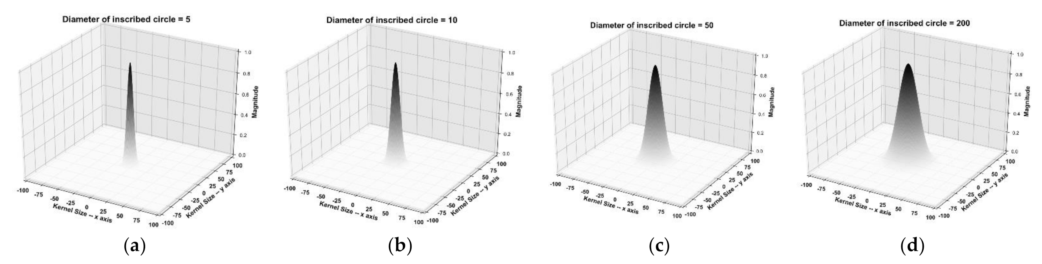To improve the model’s generalization ability to cope with possible artificial labeling errors [36] and overfitting, we employed an adaptive modified Gaussian kernel function to label smooth the center of the object with the surrounding positions. The kernel of the modified Gaussian function is the following:

$$K_m=\exp \left(-\frac{{\left(x-x_m\right)}^2+{\left(y-y_m\right)}^2}{2{\delta }^2}\right)$$

(1)

$$\mathsf{\delta }=\frac{1}{2}\frac{\min \left(W_{bo{x}_m}, H_{bo{x}_m}\right)}{Z_1}$$

(2)

($x_m$, $y_m$) is the center coordinate of ${\mathrm{m}}_{\mathrm{th}}$ object on the feature map. $W_{bo{x}_m}$ and $H_{bo{x}_m}$ are the width and height of the ground-truth bounding box. The element-wise maximum value strategy in which the same category overlaps was adopted. We charged the value of $\min \left(W_{bo{x}_m}, H_{bo{x}_m}\right)$ to cover five standard deviations under the Gaussian distribution, so the value of $Z_1$ was set to 5. Considering that the pixels contained in the actual object in the remote sensing image account for a small proportion of all of the pixels in the image, the imbalance between positive and negative samples will be severe. 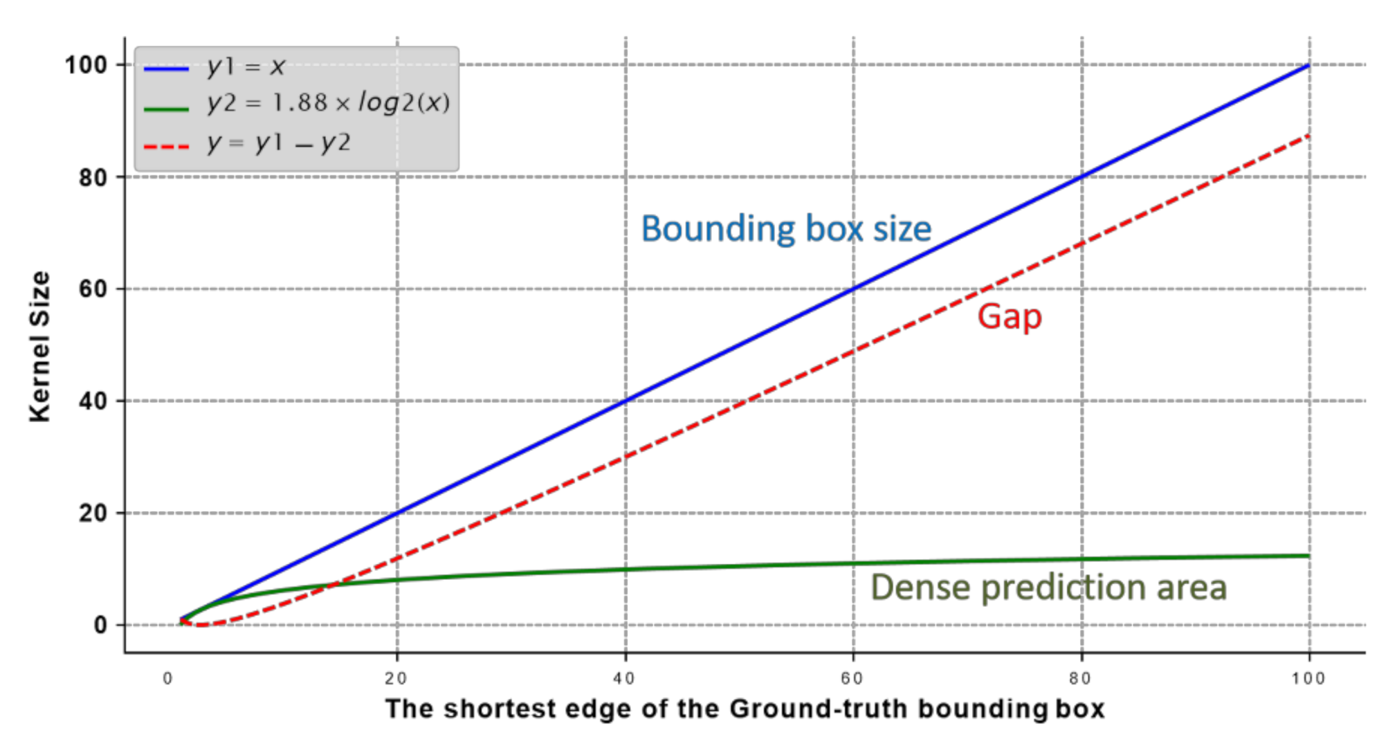Therefore, the dense prediction method [17,28] was also adopted. However, different from the former, we considered using an adaptive logarithm strategy to alleviate the gap in the size between categories. This was followed by a shape-adaptive positive sample expansion kernel as follows:

$${\mathsf{\delta }}_{plus}=\frac{1}{2}\frac{{\alpha }_{1}lo{g}_2\left(\min \left(W_{bo{x}_m}, H_{bo{x}_m}\right)\right)}{Z_1}$$

(3)

The positive sample expansion function follows the following two principles: (1) the coverage is less than or equal to $K_m$; (2) the ground-truth boundary cannot be exceeded. We treat $\min \left(W_{bo{x}_m}, H_{bo{x}_m}\right)$ as $dis$ and ${\alpha }_1$ as $x$; the above principles can be expressed in a mathematical formula as follows:

$$\left\{\begin{array}{c}f\left(x,dis\right)=dis-xlo{g}_2\left(dis\right)\ge 0\\ dis>1\end{array}\right.$$

(4)

$$\frac{\partial f\left(x,dis\right)}{\partial x}=-\frac{\ln dis}{\ln 2}<0$$

(5)

The partial derivative of the original function of the variable $x$ is always less than 0, which is a monotonic downward trend. The partial derivative for another variable $dis$ is as follows:

$$\frac{\partial f\left(x,dis\right)}{\partial dis}=1-\frac{x}{dis\ln 2}$$

(6)

$$1-\frac{x}{dis\ln 2}=0 and dis=\frac{x}{\ln 2}$$

(7)

Substitute the value of (7) into (4) and let the equation equal 0 as follows:

$$\frac{x}{\ln 2}-xlo{g}_2\left(\frac{x}{\ln 2}\right)=0$$

(8)

$$x=1.8844$$

(9)

Find the second partial derivative with respect to the variable $dis$ as follows:

$$\frac{{\partial }^{2}f\left(x,dis\right)}{\partial di{s}^2}=\frac{x}{di{s}^2\ln 2}$$

(10)

Substituting Equations (6) and (8) into Equation (9), we can obtain as follows:

$$\frac{{\partial }^{2}f\left(x,dis\right)}{\partial di{s}^2}=0.3679>0$$

(11)

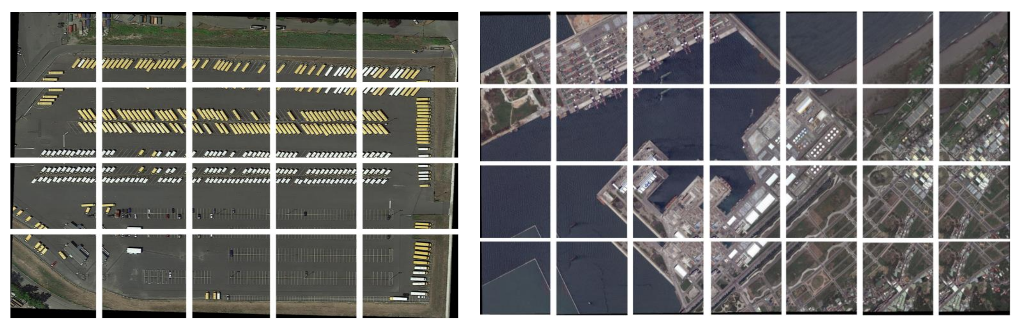
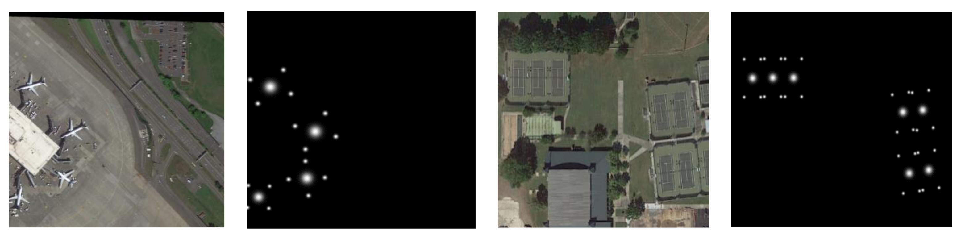
Because the second derivative is greater than 0, it is reasonable to set the value of ${\alpha }_1$ to 1.88. Figure 5 and Figure 6 show the growth of the corresponding dense prediction intervals as the size of the ground-truth box increases.

We calculated the Loss for each position in the multi-branch selection and classification head tensor, and the targets to be learned can be defined as follows:

$$Io{U}_{heat-map}={\alpha }_{3}Io{U}_1+\left(1-{\alpha }_3\right)Io{U}_2$$

(12)

$$ground-trut{h}_{heat-map}={\alpha }_{2}Io{U}_{heat-map}+\left(1-{\alpha }_2\right)K_m$$

(13)

$Io{U}_{heat-map}$ is the PQES (prediction quality estimated score) mentioned at the beginning. $Io{U}_1$ is the Intersection-Over-Union (IoU) between the predicted circumscribed bounding box and the real circumscribed bounding box; $Io{U}_2$ is the IoU between the predicted rotating bounding box and the ground truth. For all of the negative samples, the entire $Io{U}_{heat-map}$ is set to 0. The ${\alpha }_2$ and ${\alpha }_3$ are the weight factors determined in the subsequent experimental section. Taking the idea of Focal Loss [13], we propose a new modified multi-branch-aware adaptive Focal Loss function to train the model. The ground truth of the ${\mathcal{L}}_{heat-map}$ can likewise be fetched dynamically during the following training process (refer to Equations (12) and (13)):

$${\mathcal{L}}_{heat-map}=\left\{\begin{array}{c}-l\ast \left(l\ast \log p+(1-l\right)\ast \log \left(1-p\right)),l>0 \&\& l\in positive set\\ -\frac{{\theta }_{total}-{\theta }_{positive}}{4\ast {\theta }_{total}-{\theta }_{positive}}\ast {\mu }_1\ast p^{{\mu }_2}\ast \log \left(1-p\right),l=0 \left|\right| l\in negative set\end{array}\right.$$

(14)

where $l$ is the supervised value, and $p$ is the prediction. ${\theta }_{total}$ and ${\theta }_{positive}$ represent the number of all of the samples and positive samples in the feature map, respectively. We need to scale down the contribution of negative samples. ${\mu }_1$ and ${\mu }_2$ follow the Varifocal Loss [37] setting to make ${\mu }_1=0.75$, ${\mu }_2=2$.

2.3. Size Regression of Rectangle

For the regression of the circumscribed rectangle, we calculate the four distances ($l,r,t,b$) to the circumscribed rectangle bounding box from the feature points and use the GIoU [38] for training. The loss functions can be documented as follows:

$${\mathcal{L}}_{c_{reg}}=Los{s}_{GIoU}\left(bbo{x}_{pre},bbo{x}_m\right)$$

(15)

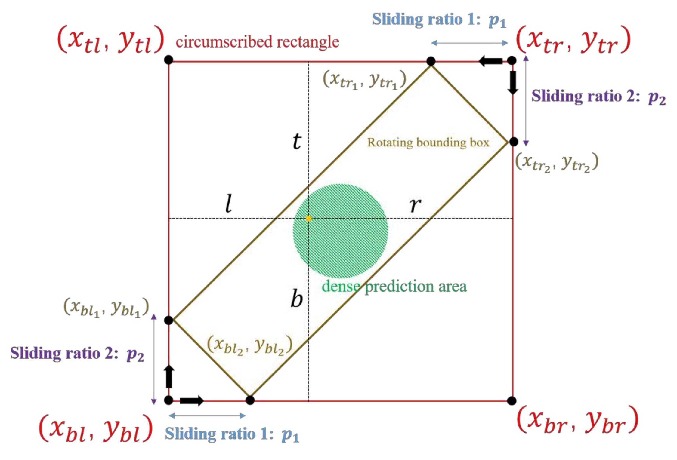
$bbo{x}_{pre}$ and $bbo{x}_m$ reprinted the $m_{\mathrm{th}}$ predicted circumscribed bounding box and the real one. Utilizing the two sliding ratios, we can deduce the coordinates of the final rotating bounding box. Using the regression method seen in Figure 4a as an example, the process looks similar to what is observed in Figure 7 as follows:

$$x_{t{r}_1}=x_{tr}-p_1\left(l+r\right)\leftrightarrow y_{t{r}_1}=y_{tr}$$

(16)

$$x_{t{r}_2}=x_{tr} \leftrightarrow y_{t{r}_2}=y_{tr}+p_2\left(t+b\right)$$

(17)

$$x_{b{l}_1}=x_{bl} \leftrightarrow y_{b{l}_1}=y_{bl}-p_2\left(t+b\right)$$

(18)

$$x_{b{l}_2}=x_{bl}+p_1\left(l+r\right) \leftrightarrow y_{b{l}_2}=y_{bl}$$

(19)

We used the Sigmoid function [39] in the model and multiplied it by a constant 0.5 to make the sliding ratios within (0,0.5) meet the following conditions ($a~d$ means the four regression ways in Figure 4):

$$\left\{\begin{array}{c}{p}_{1_{a~d}}\le \frac{1}{2}\\ p_{2_{a~d}}\le \frac{1}{2}\end{array}\right.$$

(20)

For training the sliding ratios, a new form of IoU Loss combined with Smooth L1 Loss [4] and GIoU [38] Loss called Surround-IoU Loss is adopted as follows:

$${\mathcal{L}}_{r_{reg}}=\frac{Los{s}_{SmoothL1}\left(ratio{s}_{pre},ratio{s}_{ground-truth}\right)}{\left|Los{s}_{SmoothL1}\left(ratio{s}_{pre},ratio{s}_{ground-truth}\right)\right|}Los{s}_{GIoU}\left(bbo{x}_{pre}{}^r,bbo{x}_m{}^r\right)$$

(21)

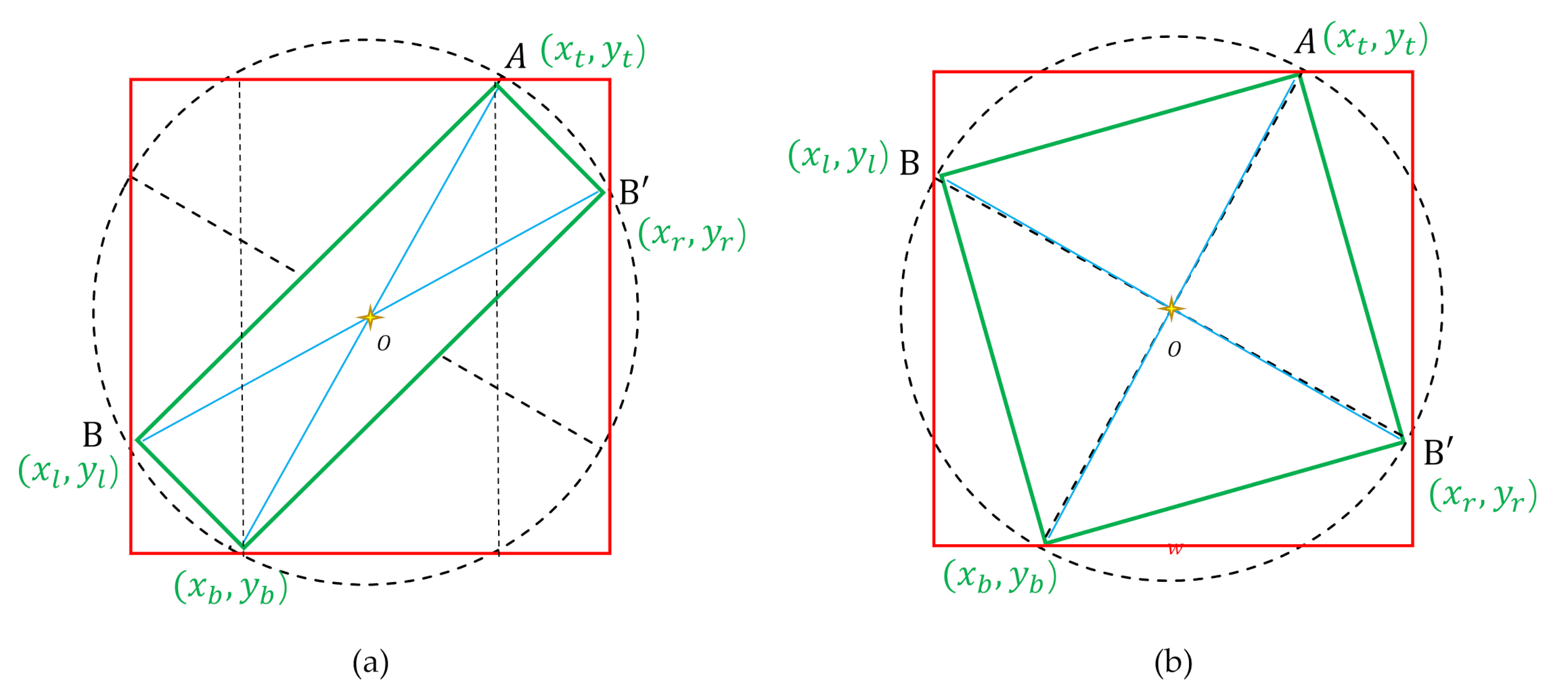
$bbo{x}_{pre}{}^r$ and $bbo{x}_m{}^r$ represent the $m_{\mathrm{th}}$ predicted rotating bounding box and the ground truth. Furthermore, the shape of the rotating bounding box cannot safely ensure a rectangular shape. As displayed in Figure 8, the soft constraints satisfy the following geometric properties:

($x_l-x_t,y_l-y_t$) represents $ve{c}_{t\to l}$, and ($x_r-x_t,y_r-y_t$) represents $ve{c}_{t\to r}$; the rest are $ve{c}_{r\to b}$ and $ve{c}_{r\to t}$. Thus, the soft constraints can be written in the following form:

$$\left(x_l-x_t,y_l-y_t\right)\cdot (x_r-x_t,y_r-y_t)=0$$

(22)

$$\left(x_b-x_r,y_b-y_r\right)\cdot \left(x_t-x_r,y_t-y_r\right)=0$$

(23)

$${\mathcal{L}}_{soft}=Los{s}_{SmoothL1}\left(ve{c}_{t\to l}\cdot ve{c}_{t\to r},0\right)+Los{s}_{SmoothL1}\left(ve{c}_{r\to b}\cdot ve{c}_{r\to t},0\right)$$

(24)

2.4. Center Vertex Attention

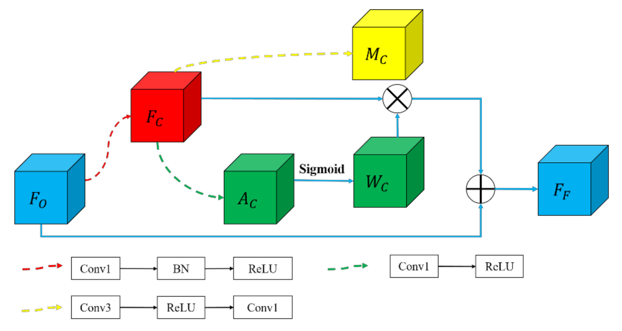
Typically, the size of a circumscribed rectangle is always greater than a horizontal one (as shown in Figure 9). As such, inspired by CBAM [40], a center vertex attention strategy should be adopted to improve the ability of the model to identify different points. We arranged the attention mechanism based on the mask at the following two sites: the center point and the four vertices of the rotating bounding box. The module architecture is portrayed in Figure 10.

$F_O$ represents the original feature map, $F_F$ represents the refined feature map, $M_C$ represents the center vertex region generated by the modified Gaussian function. The following equation expresses the fusion process and the target to be learned:

$$F_F=W_c\times F_c+F_O$$

(25)

$$Mask=\left\{\begin{array}{c}{K}_m, Center point\\ \frac{1}{2}\ast K_m, Vertex point\end{array}\right.$$

(26)

We use the same Loss function as CenterNet [16] for supervision. Moreover, SENet [41] has also been employed as the auxiliary channel attention network, and the value of the reduction ratio is 16.

The total loss function ${\mathcal{L}}_{total}$ can be written as follows (where $N$ represents the number of positive samples in an input image, and $\lambda$ is a hyperparameter for balance):

$${\mathcal{L}}_{total}=\frac{1}{N}\sum {\mathcal{L}}_{heat-map}+\frac{\lambda }{N}\sum \left({\mathcal{L}}_{c_{reg}}\ast \left({\mathcal{L}}_{soft}+{\mathcal{L}}_{mask}\right)+{\mathcal{L}}_{r_{reg}}\right)$$

(27)

3. Result and Discussion

We evaluated our model on the DOTA dataset within the PyTorch 1.7.1 + cu110 [42] framework. The training processing was deployed on a workstation with an NVIDIA Quadro RTX 5000 16 GB GPU and an Intel(R) Xeon(R) Silver 4214 CPU @ 2.20 GHz. The test processing was completed on an NVIDIA Quadro RTX 4000 GPU with 8 GB of memory.

3.1. DOTA Dataset

There were two detection tasks that were introduced to the DOTA dataset [43]. Task1 operates with the oriented bounding boxes (OBB) as the ground truth, and Task2 employs the HBB. Task1 was used for rotation detection. The dataset contains 2806 aerial images of various scales and orientations, ranging from 800 × 800 to 4000 × 4000. There are 188,282 target instances in total that are split into the following 15 categories: plane, baseball diamond (BD), bridge, ground track field (GTF), small vehicle (SV), large vehicle (LV), ship, tennis court (TC), basketball court (BC), storage tank (ST), soccer ball field (SBF), roundabout (RA), harbor, swimming pool (SP), and helicopter (HE). In order to satisfy the Surround-Net size requirements, the original input images and the corresponding labels needed to be adjusted. The step size was fixed to 100 pixels, and the window size was set to 600 pixels. After clipping there were 69,337 images in the training–verification set and 35,777 images in the test set. The decentralized detection results were combined by retaining the top 300 heat map values (the threshold is set to 0.1). Figure 11 shows part of the DOTA dataset (note that these images have been cropped).

3.2. Evaluation Indicators

We adopted the same acceptance criteria used in PASCAL VOC2007 [44] and employed means average precision (mAP) to evaluate the performance.

$$Precision=\frac{TP}{TP+FP}$$

(28)

$$recall=\frac{TP}{TP+FN}$$

(29)

$$accuracy=\frac{TP+TN}{TP+FN+FP+TN}$$

(30)

The P–R curves can be drawn according to the precomputed precision and recall of the detection results. The average precision (AP) metric is calculated by the area under the P–R curve; hence, the higher the AP value, the better the performance, and vice versa. The AP is defined as follows:

$$AP={{\displaystyle \int }}_0^{1}P(R)d\left(R\right)$$

(31)

Here, P and R represent the single-point values of precision and recall, respectively. Mean average precision (mAP) is the average of the AP in each category as follows:

$$mAP=\frac{1}{C}{\displaystyle \sum }_{C=1}^{C}AP$$

(32)

3.3. Result

3.3.1. Mask Representations

Figure 12 visualizes part of the comparison between the raw images and mask representations.

The white part of the figure represents the area where the value is not zero. In the source zone, the number is moving closer to one. In other areas, the number could be obtained using Equation (26).

3.3.2. Parameters Setting

In this section, a series of ablation experiments are performed on the DOTA validation dataset to determine the value of the hyperparameters used in Surround-Net. It is important to note that we used ResNet-50 as the backbone network for ablation experiments and set the number of training epochs to 50. The input images were resized to a resolution of 600 × 600. There were the following three hyperparameters: the weight factor $\mathit{\lambda }$ of ${\mathcal{L}}_{total}$, the weight factor ${\mathit{\alpha }}_{\mathbf{2}}$ of the $Io{U}_{heat-map}$, and the weight factor ${\mathit{\alpha }}_{\mathbf{3}}$ of the $ground-trut{h}_{heat-map}$.

• ${\mathcal{L}}_{total}$weight: We first analyzed the impact of the hyperparameters of the total loss on the detection performance. We refer to the design methods of the Loss weight in some mainstream multitasking learning models [2,3,4,5,6,7,8,9,10,11,12,13] and conducted the tests between 0.1 and 2 under the same experimental conditions. As shown in

  Table 1. Test results of different $\mathit{\lambda }$ on the DOTA validation dataset (468 images).

  $\mathit{\lambda }$	0.1	0.5	1.0	1.25	2.0
  mAP	59.015	61.242	61.292	62.031	61.589

  , $\mathit{\lambda }$ achieved the best performance when the value was 1.25. It was also observed that the detector’s performance decreases to varying degrees when the selected value is too high or too low. After adopting the GIoU and normalizing the Smooth L1, the ${\mathcal{L}}_{r_{reg}}$ was unified with ${\mathcal{L}}_{heat-map}$ in the same order of magnitude. As such, there is no necessity to downscale the regression loss. Otherwise, the model would over focus on a single task and damage the detector’s performance. Therefore, it is reasonable to employ 1.25 as the value of the hyperparameter $\mathit{\lambda }$ and adopt this value in the following experiment;
• The values of${\mathit{\alpha }}_{\mathbf{2}}$and${\mathit{\alpha }}_{\mathbf{3}}$: These two hyperparameters can be found in Equations (12) and (13). Parameter ${\mathit{\alpha }}_{\mathbf{2}}$ is used to counterbalance the value generated by the modified Gaussian kernel and the IoU between the prediction box and the ground truth box. Likewise, the parameter ${\mathit{\alpha }}_{\mathbf{3}}$ was also utilized to make a trade-off between the two different s IoU styles. One is between two horizontal bounding boxes, and the other is between two rotating bounding boxes. We restrain the range between 0 and 1 to satisfy the IoU range. Starting from intuition, parameters ${\mathit{\alpha }}_{\mathbf{2}}$ and ${\mathit{\alpha }}_{\mathbf{3}}$ were set to 0.5 when testing $\mathit{\lambda }$. Therefore, it was necessary to investigate whether other combinations could better enhance the detector’s performance. We first experimented with parameter ${\mathit{\alpha }}_{\mathbf{2}}$ and fixed the ${\mathit{\alpha }}_{\mathbf{3}}$ to 0.5. As shown in

  Table 2. Test results of different ${\mathit{\alpha }}_2$ on the DOTA validation dataset ($\mathit{\lambda }$ has been fixed to 1.25, and ${\mathit{\alpha }}_3$ has been fixed to 0.5 temporarily).

  ${\mathit{\alpha }}_2$	0.1	0.3	0.5	0.7	0.9
  mAP	61.546	61.877	62.031	61.909	61.223

  , the detector was able to achieve the best performance when parameter ${\mathit{\alpha }}_{\mathbf{2}}$ was 0.5, and there was a slight difference when other values were specified. This indicates that the proposed model can maintain classification and location consistency. In other words, the model will not have a wide gap between the classification and location scores. Similarly, the test results for the parameter ${\mathit{\alpha }}_{\mathbf{3}}$ are exhibited in

  Table 3. Test results of different ${\mathit{\alpha }}_3$ on the DOTA validation dataset ($\mathit{\lambda }$ has been fixed to 1.25, and ${\mathit{\alpha }}_2$ has been fixed to 0.5).

  ${\mathit{\alpha }}_3$	0.1	0.3	0.5	0.7	0.9
  mAP	61.641	61.773	62.031	62.116	61.845

  . However, we discovered that increasing the proportion of IoU between the horizontal bounding box results in the detector demonstrating a new optimal performance. In actuality, because a slight angular deflection can seriously reduce the IoU between rotating bounding boxes, the regression difficulty of rotating bounding boxes is more significant than that of horizontal bounding boxes, consistent with the phenomena observed in DAL [24]. Accordingly, we employed the final hyperparameters in the following experiment:${\mathit{\alpha }}_{\mathbf{2}}=0.5$, ${\mathit{\alpha }}_{\mathbf{3}}=0.7$.

3.3.3. Contributions of Several Modules in Surround-Net

In this section, we conducted ablation experiments to corroborate the contributions of the following several modules mentioned in Section 2: the soft constraint module, dense prediction module, and center vertex attention module. When evaluating the module’s effectiveness, we chose all of the DOTA datasets instead and used ResNet-152 as a backbone.

• Soft constraint module: The results are shown in

  Table 4. Results of the ablation experimental on the full DOTA dataset.

  Method	PL	BD	BR	GTF	SV	LV	SH	TC	BC	ST	SBF	RA	HA	SP	HE	mAP
  w/o Soft constraint	88.39	81.45	50.23	69.28	70.33	75.63	81.63	90.69	87.72	84.83	60.24	63.05	66.25	69.98	63.32	73.54
  w/o Dense predict	88.28	81.13	50.39	69.19	70.09	75.51	80.51	90.50	87.39	84.21	60.28	63.87	65.84	69.12	62.15	73.23
  w/o C-VAttention	88.17	80.97	49.49	68.98	69.95	75.35	80.13	90.46	86.95	83.94	59.71	62.42	65.88	69.02	63.12	72.97
  Ours	89.41	81.75	50.45	69.48	70.97	75.48	82.45	90.79	88.62	85.02	61.87	63.98	67.148	69.42	64.15	74.07

  The abbreviations of the names are defined as: PL: plane, BD: baseball diamond, BR: bridge, GTF: ground field track, SV: small vehicle, LV: large vehicle, SH: ship, TC: tennis court, BC: basketball court, ST: storage tank, SBF: soccer ball field, RA: roundabout, HA: harbor, SP: swimming pool, HE: helicopter, and mAP: means average precision.

  . The data in the first row describes how we deleted the model’s soft constraint component during the training process. That is, ${\mathcal{L}}_{soft}$ is not calculated. This reveals that the model’s performance decreases by approximately 0.7% after losing the soft constraint. Indeed, Figure 8 illustrates that soft constraints are essential for generating rectangular bounding boxes while ensuring right-angle characteristics and assisting in the regression of the sliding proportion. In addition, to further explore the effectiveness of the soft constraint module, we visualized the comparison results without adding this constraint. As shown in Figure 13, most of the bounding boxes predicted by the model in Figure 13a are parallelograms, contrary to the rectangle that we need. In Figure 13b, this phenomenon has been intensely alleviated;
• Dense predict module: The second row in the table represents the model’s performance without using the dense prediction module. The analysis in Section 2 points out that if the number of positive samples is not increased then the model will fall into overfitting because there are too few positive samples. Therefore, it can be observed from the results that the dense prediction module improves the overall performance of the model by roughly 1.13%;
• Center vertex attention module: The penultimate row in the table shows the contribution of the center vertex attention module to the overall performance. Introducing this module aims to enhance the feature extraction ability to make the model better focused on the object position and its four vertices of the corresponding rotating bounding box. It is evident that the addition of the attention module resulted in a 1.501% gain in the overall performance of the model, which further explains the necessity of an attention module in the detection tasks using remote sensing images.

3.3.4. Analysis of Surround IoU

In this section, we evaluate the effectiveness of Surround IoU Loss by comparing the stability of the Loss curve. For this experiment, the complete DOTA training set was chosen, and the number of iterations was uniformly set to 100 for comparison purposes. The Loss curve in Figure 14a depicts that a direct Smooth L1 $Los{s}_{SmoothL1}\left(·\right)$ was employed.

It should be noticed that the downward trend is not gentle, and there is a “mutation” at around the 7th iteration and the 12th iteration. Based on the analysis in Section 2, this is because direct vertex coordinate regression cannot reflect the relative position difference between the detection boxes. Therefore, we borrow the idea of calculating the Loss in a rotating bounding box in SCRDet [25] by introducing normalization and IoU information. The image in Figure 14b shows the Loss during the training process after replacing the original Loss function with Surround IoU, and it is obvious that the Loss curve becomes more flattened than the former.

3.3.5. Analysis of Multi-Branch Regression

This subsection discusses the impact of the proposed multi-branch prediction structure on model performance. According to the discussion in Section 2, there are the following four types of regression branches: oriented primary diagonal slender rectangular regression, oriented minor diagonal rectangular slender regression, oriented primary diagonal rectangular regression, and oriented minor diagonal rectangular regression. The model’s validity can be verified by masking some branches artificially. In the following experiments, we compared the performance by means of shielding in the Figure 4a,b branch and in the Figure 4c,d branch. The results and visual analysis are provided in

Table 5. The experimental results of shielding different regression branches.

Method	PL	BD	BR	GTF	SV	LV	SH	TC	BC	ST	SBF	RA	HA	SP	HE	mAP
Shielded branch a~b	88.89	81.26	42.68	69.13	51.39	55.25	64.67	86.48	83.21	84.88	54.13	63.71	51.70	67.17	62.72	67.15
Shielded branch c~d	78.86	67.72	50.32	68.25	70.73	75.32	81.82	90.18	88.45	66.65	61.66	50.44	67.01	69.31	57.67	69.63
SurroundNet	89.41	81.75	50.45	69.48	70.97	75.48	82.45	90.79	88.62	85.02	61.87	63.98	67.148	69.42	64.15	74.07

and Figure 15.

We completed the testing process by zeroing the different branches on the prediction tensor and picking a new maximum value in the remaining branches. According to the results in Table 5, keeping only some of the branches will significantly impair the model’s performance. It is observed that if only the branches in Figure 4a,b are kept, the AP values of the large vehicle, small vehicle, ship, and harbor categories show a relatively colossal drop compared to the best performance. However, if only the branches in Figure 4c,d are kept, then the AP values for the roundabout, basketball court, and storage tank categories show the same decline. In the first row of pictures in Figure 15, the first two represents the prediction results for when only branches c-d are kept, and the last two represent the results obtained when only branches a–b are kept. Compared to keeping all of the branches in the second row, the detection boxes for the harbor and large vehicle categories only showed regression in directions c–d, showing a high level of redundancy. Moreover, in the large vehicle category, many objects are missed by NMS [45]. In the last two pictures in the first row, since the regression can only be carried out in the a-b directions, the obtained detection boxes cannot completely cover the target, resulting in a shallow IoU with the ground truth. It can be seen from the results in the second row, which multi-branch regression can adaptively select the appropriate detection box.

3.3.6. Comparisons with State-of-the-Art Detectors

In this part, we compare Surround-Net with other state-of-the-art detectors on the DOTA dataset and obtain the FPS results shown in

Table 6. Evaluation results of detection on the DOTA test dataset. ’*’ means using multi-scale training and multi-scale testing. ‘$†$’ means that only multi-scale testing was used.

Methods	PL	BD	BR	GTF	SV	LV	SH	TC	BC	ST	SBF	RA	HA	SP	HE	mAP
Faster R-CNN-O(A) [20]	88.44	73.06	44.86	59.09	73.25	71.49	77.11	90.84	78.94	83.90	48.59	62.95	62.18	64.91	56.18	69.05
SCRDet(A) [25]	89.98	80.65	52.09	68.36	68.36	60.32	72.41	90.85	87.94	86.86	65.02	66.68	66.25	68.24	65.21	72.61
RSDet (A) [31]	90.13	82.01	53.83	68.52	70.21	78.73	73.60	91.22	87.13	84.71	64.31	68.21	66.14	69.31	63.74	74.12
Gliding Vertex(A) [26]	89.64	85.00	52.26	77.34	73.01	73.14	86.82	90.74	79.02	86.81	59.55	70.91	72.94	70.86	57.32	75.02
CSL(A) [21]	90.25	85.53	54.64	75.31	70.44	73.51	77.62	90.84	86.15	86.69	69.60	68.04	73.83	71.10	68.93	76.17
$R^3$Det *(A) [19]	89.80	83.77	48.11	66.77	78.76	83.27	87.84	90.82	85.38	85.51	65.67	62.68	67.53	78.56	72.62	76.47
ReDet *(A) [46]	88.81	82.48	60.83	80.82	78.34	86.06	88.31	90.87	88.77	87.03	68.65	66.90	79.26	79.71	74.67	80.10
Oriented R-CNN *(A) [47]	89.84	85.43	61.09	79.82	79.71	85.35	88.82	90.88	86.68	87.73	72.21	70.80	82.42	78.18	74.11	80.87
O2DNet(AF) [28]	89.31	82.14	47.33	61.21	71.32	74.03	78.62	90.76	82.23	81.36	60.93	60.17	58.21	66.98	61.03	71.04
DRN(AF) [48]	89.71	82.34	47.22	64.10	76.22	74.43	85.84	90.57	86.18	84.89	57.65	61.93	69.30	69.63	58.48	73.23
SAR(AF) [27]	90.89	82.67	49.75	69.90	68.07	72.31	81.24	90.27	88.19	82.43	62.08	66.43	66.20	68.34	63.48	73.48
CenterRot(AF) [49]	89.74	83.57	49.53	66.45	77.07	80.57	86.97	90.75	81.50	84.05	54.14	64.14	74.22	72.77	54.56	74.00
MEAD(AF) [50]	88.42	79.00	49.29	68.76	77.41	77.68	86.60	90.78	85.55	84.54	62.10	66.57	72.59	72.84	59.83	74.80
CFA *(AF) [51]	89.26	81.72	51.81	67.17	79.99	78.25	84.46	90.77	83.40	85.54	54.86	67.75	73.04	70.24	64.96	75.05
BBAV *(AF) [30]	88.63	84.06	52.13	69.56	78.26	80.40	88.06	90.87	87.23	86.39	56.11	65.62	67.10	72.08	63.96	75.36
AROA *(AF) [52]	88.33	82.73	56.06	71.58	72.98	77.59	78.29	88.63	83.33	86.61	65.93	63.52	76.03	78.43	61.33	75.41
DAFNe *(AF) [53]	89.40	86.27	53.70	60.51	82.04	81.17	88.66	90.37	83.81	87.27	53.93	69.38	75.61	81.26	70.86	76.95
SurroundNet-101(AF)	88.92	81.02	49.42	68.13	69.28	73.51	80.29	88.56	86.45	83.04	60.18	62.62	66.12	68.69	63.66	72.66
SurroundNet-152(AF)	89.41	81.75	50.45	69.49	70.97	75.49	82.46	90.80	88.64	85.02	61.87	63.98	67.15	69.42	64.15	74.07
SurroundNet-152 †(AF)	90.03	83.66	52.70	70.50	74.19	77.33	84.79	90.91	89.34	86.79	63.68	66.37	71.68	70.53	65.68	75.88

Number 101 indicates that the backbone network is ResNet101, and 152 indicates that the backbone network is ResNet152.

and

Table 7. Inference speed comparisons with other methods.

Methods	$\mathrm{SCRDet}$	$R^2\mathrm{CNN}$	$\mathrm{BBAVector}$	$\mathbf{\text{SurroundNet-152}}$	$\mathrm{O}2\mathrm{DNet}$-101
FPS	2.23	2.73	10.32	12.57	13.89

All models were tested under the same conditions. GPU: Quadro RTX 4000 $\times$ 1. Input resolution: 800 $\times$ 800.

. Furthermore, we randomly selected some of the detection results shown in Figure 16.

During the experiment, Surround-Net used both ResNet-101 and ResNet-152 as the backbone and multi-scale testing to achieve the best performance. As shown in Table 6, the detectors are divided into the following two groups: anchor-based (A) and anchor-free (AF) detectors. Table 6 indicates that ResNet-152 performs better than ResNet-101, so there is a heavy dependence on feature extraction.

Overall, although lower than some anchor-based two-stage models and anchor-free models, Surround-Net still obtained competitive results (75.88 mAP) and maintained a high processing speed (12.57 FPS), resulting in a performance trade off. In particular, compared to the eight-parameter models [26,27,28,29,30,31,32], Surround-Net still achieves state-of-the-art results, confirming the correctness of the method in solving boundary problems. Table 7 shows the FPS results that were obtained under the same test conditions. It can be seen that Surround-Net-152 still has 12.57 FPS, showing the efficiency of our model. Figure 16 reflects that Surround-Net can not only complete high-precision detection for horizontal objects but also achieve excellent results when applied to objects with a high aspect ratio.

4. Final Discussion and Conclusions

After analyzing the ranking problems and regression discontinuity problems in the five-parameter and eight-parameter models, we introduced a new one-stage anchor-free model with multi-branch prediction for oriented detection tasks. In order to maintain consistency between classification, localization, and branch selection, we replaced the original classification label with the corresponding PQES (prediction quality-estimated score). Further, we added center vertex spatial attention to ensure that our model fully utilizes features to distinguish the foreground from the background. The soft constraint was also proposed to refine the bounding box. At the same time, to improve the prediction recall and to alleviate the imbalance between positive and negative samples in the anchor-free model, we also adopted a dense prediction strategy.

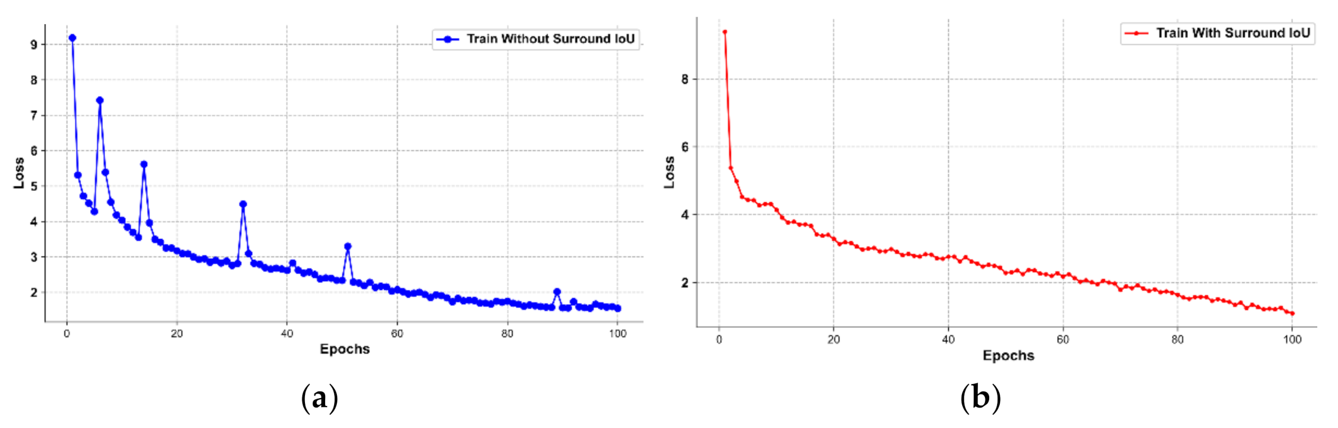
In the experiment, we first discussed the impact of the weights of the Loss function. The experiments show that the Loss weight $\lambda$ should be 1.25, and in PQES, the weights of ${\alpha }_2$ and ${\alpha }_3$ should be set to 0.5 and 0.7. Further, we investigated the influence of our three proposed modules. The soft constraint module results in a performance enhancement of 0.7%, and more importantly, it enables the model to output a rectangular detection box that meets the geometric requirements. The dense prediction module improves the performance by 1.13%, while the attention mechanism model improves it by 1.501%. In order to enhance the smoothness of the Loss curve, we adopted the Surround IoU Loss by incorporating location information to train the sliding ratio. In addition, we also conducted experiments and discussions on the effectiveness of multi-branch prediction, which showed that a single regression method will damage the detector’s performance in terms of oriented detection. Finally, we compared the results with the state of the art and visualized the detection results. It can be seen that the model proposed in this paper achieved values of 75.88 mAP and 74.07 mAP at 12.57 FPS, which is a competitive result and represents a trade-off between performance and running speed.

However, it should be noted that there is still a slight gap between Surround-Net and the state of the art. In the anchor-based and two-stage models [19,20,21,25,26,31,46,47] listed in Table 6, the best Surround-Net performance is in a position that is higher than the middle of the ranking list. In the anchor-free and one-stage models [27,28,30,48,49,50,51,52,53], the values representing the best performance in our work are only lower than those achieved by DAFNE [53]. 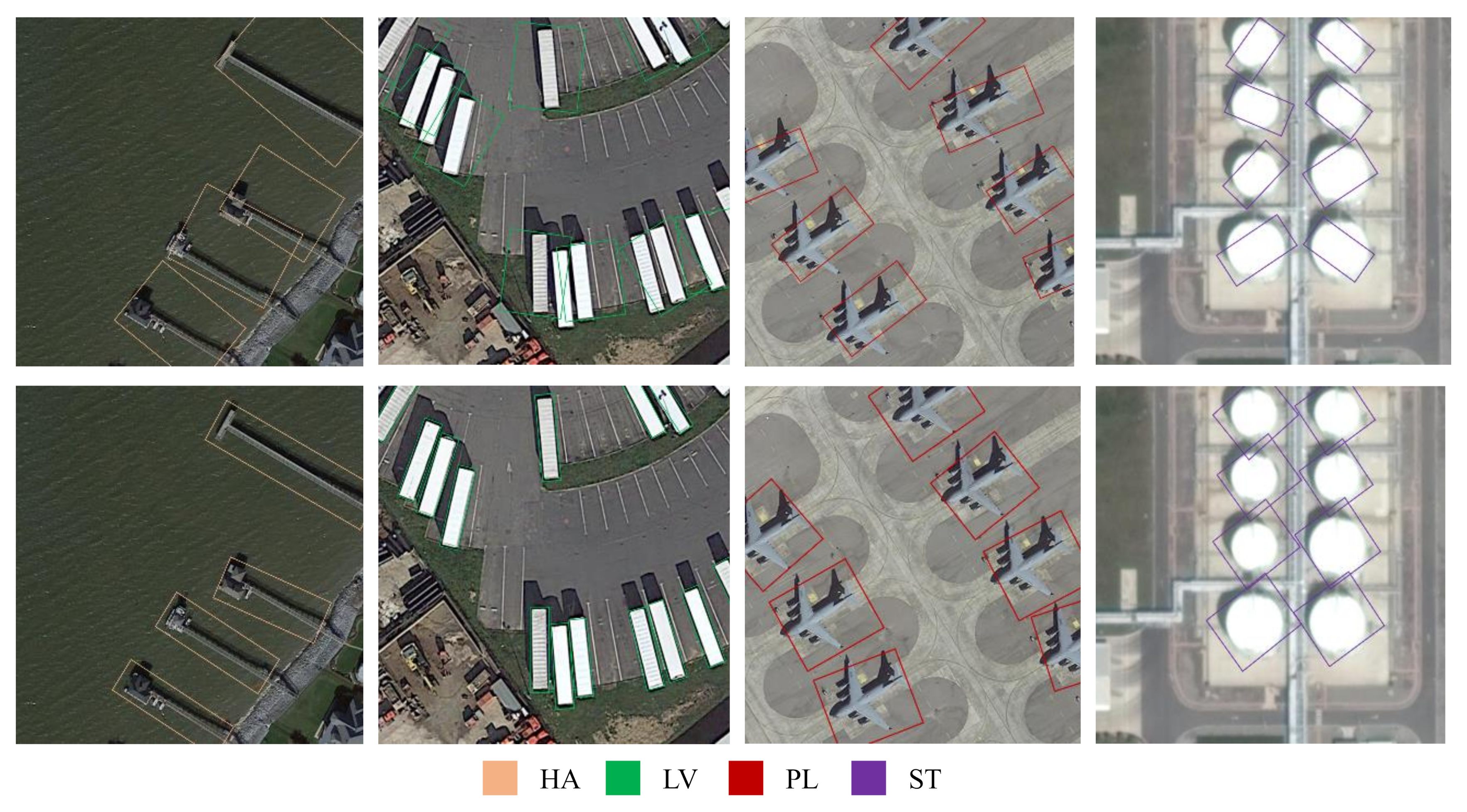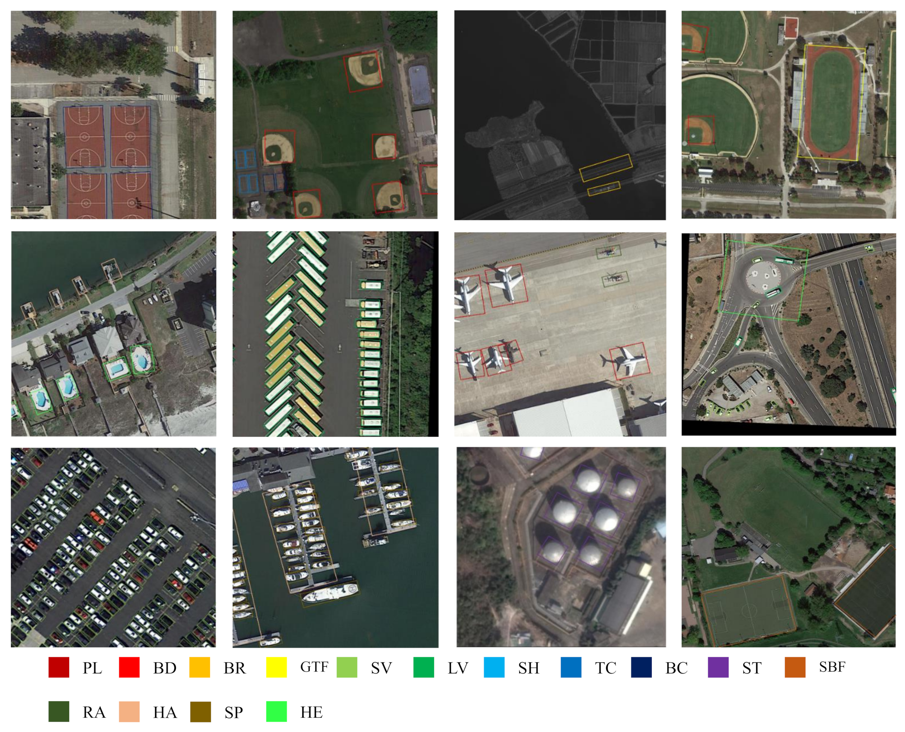However, when multi-scale testing technology is not used and Resnet-101 is used as the backbone, the performance of Surround-Net-101 (72.66%) is better than that of DAFNE-101 [53] (70.75%). In addition, we found a few missed detections (which occur in the first two pictures in the last line of Figure 16) in some specific categories (Small Vehicle and Ship). It is because the output feature map undergoes 4-fold down-sampling, and some objects may share the same center. As such, reducing the probability of missed detection is particularly important for our future research.