Article

Consolidated Convolutional Neural Network for Hyperspectral Image Classification

1
Department of Electrical Engineering, National Taipei University of Technology, Taipei 10608, Taiwan
2
Department of Communications, Navigation and Control Engineering, National Taiwan Ocean University, Keelung City 202301, Taiwan
3
Center for Space and Remote Sensing Research, National Central University, Taoyuan 32001, Taiwan
4
Department of Computer Science & Information Engineering, National Central University, Taoyuan 32001, Taiwan
*
Author to whom correspondence should be addressed.
Remote Sens. 2022, 14(7), 1571; https://doi.org/10.3390/rs14071571
Submission received: 18 February 2022 / Revised: 14 March 2022 / Accepted: 22 March 2022 / Published: 24 March 2022

Abstract

:
The performance of hyperspectral image (HSI) classification is highly dependent on spatial and spectral information, and is heavily affected by factors such as data redundancy and insufficient spatial resolution. To overcome these challenges, many convolutional neural networks (CNN) especially 2D-CNN-based methods have been proposed for HSI classification. However, these methods produced insufficient results compared to 3D-CNN-based methods. On the other hand, the high computational complexity of the 3D-CNN-based methods is still a major concern that needs to be addressed. Therefore, this study introduces a consolidated convolutional neural network (C-CNN) to overcome the aforementioned issues. The proposed C-CNN is comprised of a three-dimension CNN (3D-CNN) joined with a two-dimension CNN (2D-CNN). The 3D-CNN is used to represent spatial–spectral features from the spectral bands, and the 2D-CNN is used to learn abstract spatial features. Principal component analysis (PCA) was firstly applied to the original HSIs before they are fed to the network to reduce the spectral bands redundancy. Moreover, image augmentation techniques including rotation and flipping have been used to increase the number of training samples and reduce the impact of overfitting. The proposed C-CNN that was trained using the augmented images is named C-CNN-Aug. Additionally, both Dropout and L2 regularization techniques have been used to further reduce the model complexity and prevent overfitting. The experimental results proved that the proposed model can provide the optimal trade-off between accuracy and computational time compared to other related methods using the Indian Pines, Pavia University, and Salinas Scene hyperspectral benchmark datasets.

Graphical Abstract

1. Introduction

Hyperspectral images (HSIs) have been found in a number of applications in the field of remote sensing such as vegetation monitoring [1,2,3], area change detection [4,5], and atmospheric research [6,7]. Hyperspectral sensors generate hundreds of wavelength bands that range from the visible to the near-infrared spectrum [8]. These wavelength bands typically provide rich spectral and spatial information for analyzing the target area [9]. Each pixel in a HSI corresponds to hundreds of reflected electromagnetic radiation bands [10]. However, this large number of wavelength bands contains nonlinear and high-dimensional features which make the analysis of HSIs even more challenging [11]. Lately, principal component analysis (PCA) [12] and kernel PCA [13,14] techniques have been proposed to overcome the dimensionality and nonlinear problem in the field of hyperspectral images classification, respectively. Although these techniques showed a great success in dimensionality reduction, they have some limitations in feature extraction for HSIs classification [15]. HSIs classification is always one of the key topics in the field of remote sensing. Traditional machine learning algorithms such as support vector machines (SVM) [16], random forest [17], multinomial logistic regression [18], and k-nearest neighbor [19,20] have been widely used for hyperspectral image classification. However, the complex characteristics and nonlinearity of HSIs make the classification of HSIs a challenging task for the traditional machine learning methods [21]. Unlike these traditional machine learning methods that require extensive domain knowledge, debugging skills, and hand-crafted features, convolutional neural networks (CNNs) have shown very promising results in HSI classification in recent years [21,22,23,24,25]. CNNs use a series of hierarchical layers to extract informative features from the HSIs. Shallower layers extract features such as edge and texture features, while the deeper layers extract more complex features [26]. The learning process and features extraction from high-dimensional data are automatic, which makes CNNs more suitable for complex applications in the field of remote sensing such as scene classification and object detection [27,28,29,30]. The structure of CNNs typically consists of a stack of convolution layers and pooling layers, and a fully connected layer. In the convolutional layers, the image spatial information is extracted by a set of filters. Then, the pooling layers reduce the spatial size of the feature maps created by the convolutional layers to produce more abstract features. Finally, these feature maps are further flattened into a feature vector and fed to a fully connected layer [31,32]. However, CNN architectures require a large number of training samples to avoid issues, such as overfitting and vanishing gradient [33,34]. Usually, techniques such as data augmenting [35] and Dropout regularization [36] have been used to reduce the impact of such issues. Moreover, CNNs are computationally intensive and require a large amount of memory [37]. Recently, graphics processing units (GPUs) have been used to boost the CNNs performance on HSI classification [38,39]. Hyperspectral images classification using CNNs has been extensively studied in recent years.
One study [40] introduced a method based on adaptive dimensionality reduction (ADR) and a semi-supervised 3D convolutional neural network (SS-3DCNN) for hyperspectral images classification. The proposed approach seeks to solve the curse of dimensionality problem and the limited number of training samples by finding the most informative spectral bands using labeled and unlabeled training samples. Then, the selected bands are fed into a semi-supervised encoder-decoder 3-D CNN for HSI classification. Zhang et al. [41] proposed a lightweight spectral–spatial attention fusion with a deformable convolution residual network (SSAF-DCR) for HSI classification. The proposed model is composed of both end-to-end sequential deep feature extraction and a classification network, which led to improvement in the HSI classification performance. The spectral and low-level spatial features of HSIs are extracted with a 3D CNN, and the high-level spatial features are extracted by a 2D CNN. The effectiveness of the SSAF-DCR approach was clearly proven. Another interesting work [42] proposed a deep spectral spatial inverted residuals network (DSSIRNet) for hyperspectral images classification. The proposed DSSIRNet introduced a data block random erasing technique to overcome the lack of labeled samples by augmenting small spatial blocks. Moreover, a deep inverted residuals (DIR) module for spectral spatial feature extraction is proposed. Furthermore, a global 3D attention module is implemented and embedded into the DIR module. The module considers the global context features of spectral and spatial dimension to further improve the classification performance.
Nevertheless, the performance of the HSIs classification is still negatively impacted by factors such as data redundancy, insufficient spatial resolution, and limited labeling samples. This study proposes a C-CNN structure, which aims to resolve the aforementioned issues and achieve satisfactory accuracy. Moreover, it aims to accelerate the computing processes and provide faster response time for the HSI classification. Meanwhile, the use of high-performance computing (HPC) methods is evaluated to improve the computing process for the HSI classification. The contributions of this study can be summarized as follows:
1.
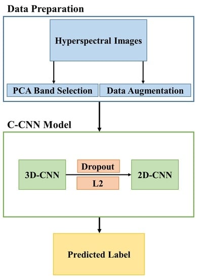
This paper proposes a consolidated convolutional neural network (C-CNN) that is comprises of a three-dimensional CNN (3D-CNN) joined with a two-dimension CNN (2D-CNN) to produce sufficient accuracy and reduce the computational complexity for HSIs classification.
2.
PCA has been used to reduce the spectral bands of the input HSIs.
3.
Image augmentation methods including rotation and flipping have been applied to increase the number of training samples and reduce the impact of overfitting.
4.
Dropout and L2 were adopted to further reduce the model complexity and prevent overfitting.
5.
The influence of band selection and training sample ratio on the overall accuracy (OA) was investigated.
6.
The impact of window size and multi-GPUs on the OA and processing time was also examined.

2. Methodology

In the traditional 2D-CNNs, the convolutional filter is normally applied to HSI on the spatial level instead of the spectral level. On the other hand, in the 3D-CNNs, convolutional kernel can be used to simultaneously extract spatial and spectral features from the HSI data. However, the computational complexity of the 3D-CNN convolutional kernel can be very high. The previous methods that combined both 2D-CNN and 3D-CNN have demonstrated a certain level of improvement. However, there is still a room for computational complexity and performance improvement. Both spatial and spectral information are expected to be extracted together for performing a better HSI classification result.

2.1. Proposed Model

By the 2D-CNN of the proposed model, the 2D convolutional filter extracts features from the local neighborhood of the previous feature map and applies an added bias value before passing the result to an activation function. Formally, at position (x, y) on the ith layer and jth feature map, the unit value is expressed as v i j x y , and is given by the following Equation (1) [43]:
v i j x y = g b i j + m p = 0 P i 1 q = 0 Q i 1 w i j m p q v i 1 m x + p y + q
where g is the sigmoid activation function, b is a bias value for the feature map, m is a position set from ( m 1 ) th layer feature map connected to the current feature map, w i j m p q is the weight value at the nuclear position (p, q) connecting the mth feature map, and P i and Q i are the height and width of the kernel.
In the down-sampling layer on the feature map of the previous layer, it can increase the invariance of the input distortion by pooling of the local neighborhood and by reducing the feature map resolution. Then, the CNN architecture can be constructed by stacking multiple convolutional and down-sampling layers in an alternating manner. In the 2D-CNN, when dealing with spectral analysis, it is necessary to extract features among different wavelength spectra. For this purpose, during the convolutional phase of CNN, a 3D convolution operation is performed to simultaneously extract features from both spatial and spectral dimensions. The 3D convolution operation is implemented by convolving a cube formed by stacking a plurality of consecutive bands with a 3D core, and by having the feature map on the convolution layer be connected to a plurality of consecutive bands of the previous layer to extract spectral features. Formally, at the (x, y, z) position of the ith layer and the jth feature map, the unit value is given by the following Equation (2):
v i j x y z = g b i j + m p = 0 P i 1 q = 0 Q i 1 r = 0 R i 1 w i j m p q r v i 1 m x + p y + q ( z + r )
where R i represents the size of the 3D convolution kernel in the spectral dimension, and w i j m p q r is the value of the (p, q, r) of the kernel of the mth feature map connected to the previous layer.
The proposal structure of C-CNN model for hyperspectral image classification is illustrated in Figure 1. The proposed C-CNN structure consists of 3D convolutional layers, 2D convolutional layers, fully connected (FC) layers, and Softmax output layer, where 3D-CNN is used to extract both spectral and spatial features, and the 2D-CNN is used to further extract more spatial features. In addition, the placement of the Max-pooling in the 3D-CNN and the 1 × 1 convolutions in the 2D-CNN with data augmentation are introduced in the proposed model to reduce the computational complexity and produce better performance. Additionally, because of the common problem of overfitting in deep neural networks especially with high-dimensional data, methods such as rectified linear unit (ReLU) [44], L2 regularization [45] and Dropout [46] have been adopted in this study. In the proposed network, the HSI is expressed as I R M * N * D , where I is the original input, M is the width, N is the height, and D is the number of spectral bands. Each pixel in I contains D spectral values. It uses the one-hot tag vector to represent the output as Y = ( y 1 , y 2 , , y C ) R 1 * 1 * C , where C represents the number of land cover categories.
Since pixels in hyperspectral images are usually mixed with land cover categories, it is a huge challenge to accurately classify a category corresponding to each pixel for any model. In order to eliminate spectral redundancy, the PCA is firstly applied to the original HSI data (I). The PCA is employed to reduce the number D of spectral bands while maintaining the same spatial size, i.e., M as the width and N as the height. We only reduce the spectral band and retain the important spatial information in the HSI classification. After the PCA reduces the number of bands, we use X R M * N * B to represent its spectral image, where X is the input after the PCA dimensionality reduction, M is the width, N is the height, and B is the number of bands after the dimension is reduced by the PCA band selection ratio ( λ ). After the PCA band reduction, the 3D-CNN uses a 3D kernel for 3D convolution operations to extract both spatial and spectral features simultaneously. The proposed model C-CNN is deployed with the number and size of the 3D convolutional kernel on the 3D convolutional layer. In the proposed model, there are three 3D convolution layers for learning the spectral information with different scales. The deployments are set with 8, 3 × 3 × 7 convolution kernels on the first layer, 16, 3 × 3 × 5 convolution kernels on the second layer, and 32, 3 × 3 × 3 convolution kernels on the third layer.
In order to provide invariance to the proposed model, a Max-pooling function was performed after all the 3D convolutions as the down-sampling process to reduce the resolution of the feature map. Each pooling layer corresponds to the previous convolution layer, and the neurons on the pooling layer are combined by the specified block size on the convolutional layer. It is used after the third 3D convolutional layer. Since the size of the feature maps can be reduced without losing any feature information, the convergence of the network can be well facilitated with less amount of computations on the feature map with the size S 2 × S 2 × B 2 × 32 after the Max-pooling, and the processing time for the classification can be facilitated and optimized. Prior to switching into the 2D domain, since the 2D convolution input must be of three-dimensional for fulfilling the process, the feature map must be reshaped to be 3-dimensional with the size of S 2 × S 2 × ( B 2 × 32 ) as the input of the 2D convolutional layer, where the ( B 2 × 32 ) is the number of channels in the 2D convolutional input feature maps.
Due to the large number of channels, the increase of computing complexity is the concern for further 2D convolution operations. The 1 × 1 convolutions are deployed to reduce both the size of convolutional kernels and the complexity of the model without losing the representation of the model feature. Meanwhile, because a simple convolution operation easily leads to overfitting, the deployment of 1 × 1 convolutions can also get better generalization and learning ability. The number and size of 2D convolution kernels on the 2D convolutional layer are deployed as 128, 1 × 1 convolution kernels on the first layer, 256, 3 × 3 convolution kernels on the second layer, and 64, 1 × 1 convolution kernels on the third layer, respectively, as shown in Figure 1. Maintaining an appropriate representation is very important for HSI classification. For increasing the number of spectral–spatial feature maps, the 3D convolution is applied three times, by which the spectral information in the input HSI data can be well preserved. Per the data process flow, the 2D convolution is also applied three times before stepping into the Flatten layer, by which the spatial information in different spectral bands can be distinguished without the loss of substantial spectral information.

2.2. Training and Testing Process

During the training process, the training samples are randomly divided into a number of N batches, and each batch contains the same number of samples. The training is performed by using a random gradient descent method. For each iteration, only one batch is sent to the network for training. The training process does not stop until the specified number of iterations is reached. During the testing process, test samples are sent to the trained network and the predicted labels can be obtained by finding the maximum value in the output vector. The training and testing process flow chart of the proposed model C-CNN is shown in Figure 2.

2.3. Data Augmentation

Due to the lack of training samples, the learning model can be easily overfit. Hence, in order to reduce the impact of overfitting, one of the most common methods is to produce a slightly modified version of the existing training samples to increase the number of training samples. This production operation is known as data augmentation or image augmentation. In the experiment, each pixel was treated as a center and its neighbor S × S pixel block was taken as a sample, hence the data size of each sample is S × S × B. For every training sample, a rotation by 90 , 180 , and 270 has been performed as the conversion to have 4 samples including the original one, and then these samples are flipped vertically to form 8 samples in total. The proposed model trained on the augmented datasets is called C-CNN-Aug.

3. Experimental Results

This section introduces the experimental environment, the impact of PCA ratio λ on the overall accuracy (OA), the results of varying the window size, the comparative results of other HSI classification methods, the impact of training sample ratio on the OA, and the impact of multi-GPUs implementation on the processing time, respectively.

3.1. Experimental Environment and Parameter Settings
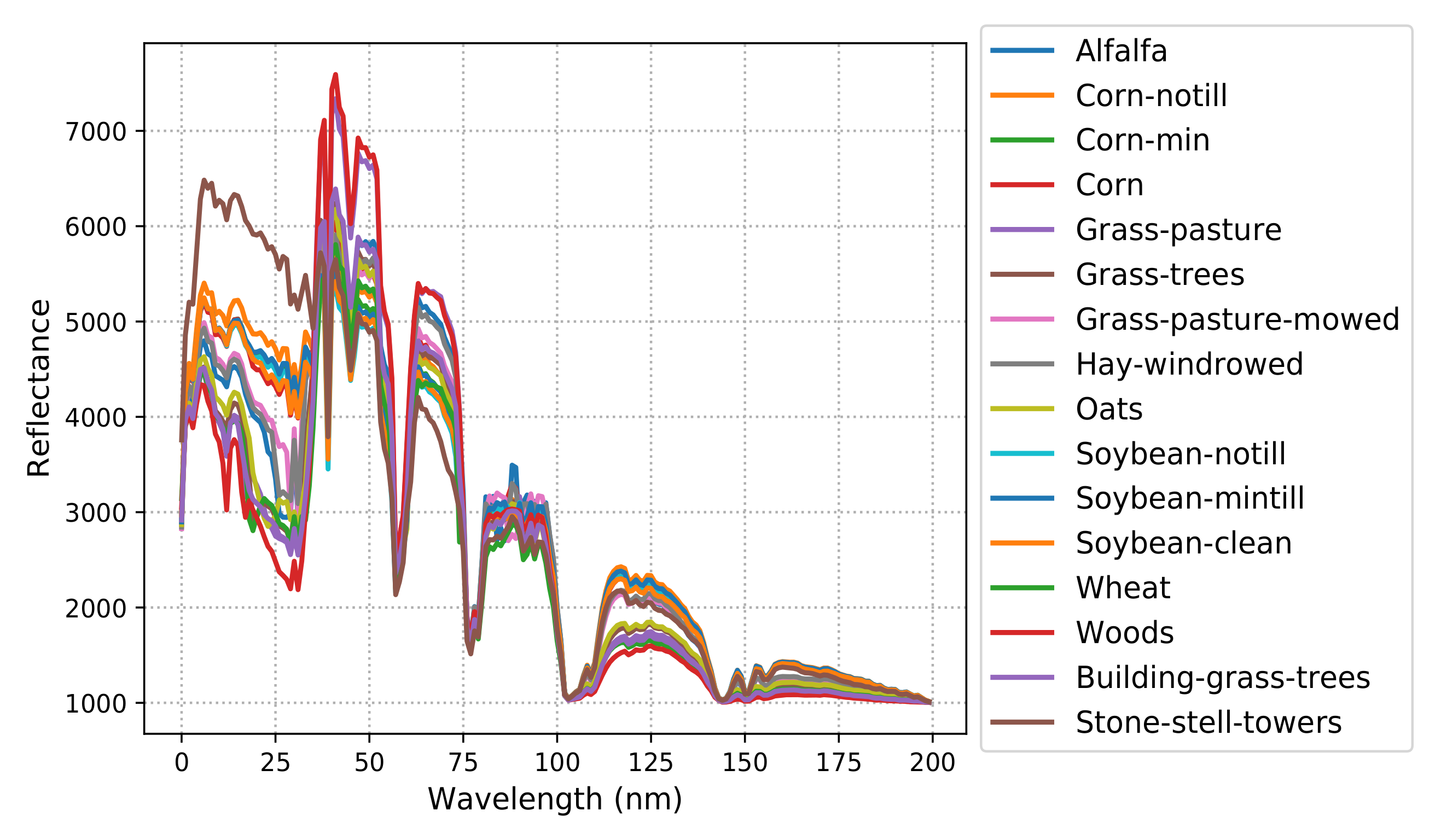
The hardware environment in which all experiments are performed has Intel Xeon (R) CPU E5-2630 v4 processors with 64 GB of DDR4 RAM. The graphics processing unit (GPU) is NVIDIA GeForce RTX 2080 Ti with 11 GB of memory. The software environment is set up with Ubuntu 16.04.4, 64-bit as the operating system, CUDA 9, cuDNN 5.1.5, TensorFlow 1.13.1, and Python 3.6. The datasets are randomly divided into a training set and testing set in a ratio of 1% and 99%, respectively. In addition, all the network weights were randomly initialized, and the adaptive moment estimation (Adam) [47] was employed as the optimization strategy. The initial learning rate was set at 0.001, and the mini-batch size was 128.

3.2. Datasets

Three benchmark datasets are used to evaluate the performance of our proposed models. They are namely Indian Pines (IP), Pavia University (PU), and Salinas Scene (SA). These three datasets are collected by the airborne visible infrared imaging spectrometer (AVIRIS), reflective optics system imaging spectrometer (ROSIS), and AVIRIS sensor in the Salinas Valley, California, respectively. The detail information of each dataset is shown in Table 1, where the column Discarded Bands depicts the number of the bands covering water. In practical applications, the labeled samples are usually very limited, which makes HSI classification more challenging. Therefore, in order to present the performance of our proposed method under a condition of small sample size, we randomly selected 1% of each class to form a training set, and the remaining samples made up for the testing set. The semantics and labels of the Indian Pines, Pavia University, and Salinas Scene datasets have been shown in Figure 3, Figure 4 and Figure 5, respectively.

3.3. The Impact of PCA Band Selection Ratio on Overall Accuracy

The influence of band selection ratio λ of PCA on the OA was examined in this section. For example, the band selection ratio, λ = 0.10 represents 10% of the most informative selected band, and the higher λ indicates the selected data is more similar to the original data. However, the higher the λ value is, the more computational power is required. The appropriate λ value was empirically determined by the best OA in the band selection ratio analysis in Table 2. In fact, the appropriate λ value is not only determined by the OA, but also by the computational complexity as shown in Table 3. Therefore, there is a trade-off between the OA and computational complexity when the optimal λ value is determined. Table 2 shows the λ value ranges from 0.01 to 0.10, and their OAs are presented using IP, PU, and SA datasets, respectively. For the IP and PU datasets, the optimal OA is λ = 0.10 and λ = 0.08, respectively. For the SA dataset, the OA reached to 99% at λ = 0.03, and continued rising up to 99.43% at λ = 0.10. Therefore, λ = 0.10, 0.08, and 0.10 are selected in this experiment for IP, PU, and SA datasets, respectively.

3.4. The Impact of Window Size on Overall Accuracy and Processing Time

The impact of window size S × S on the model performance is shown in Table 3. From Table 3 and Figure 6 below, it is found that the performance of 5 × 5 size is lower than those of other sizes. The performance of 15 × 15 size shows significant improvement compared with that of 5 × 5 size. Nevertheless, there is no much difference among 15 × 15, 25 × 25, and 35 × 35 sizes in terms of OA. The 15 × 15 was finally decided in this study as it turns out that the 15 × 15 window size provides the best trade-off between the overall accuracy and testing time.

3.5. Comparison with Other Methods

In order to compare the performance of the proposed models with the-state-of-art models, such as SS-3DCNN [40], SSAF-DCR [41], and DSSIRNet [42], for the hyperspectral image classification, the experimental results with each benchmark dataset are addressed in the subsections below.

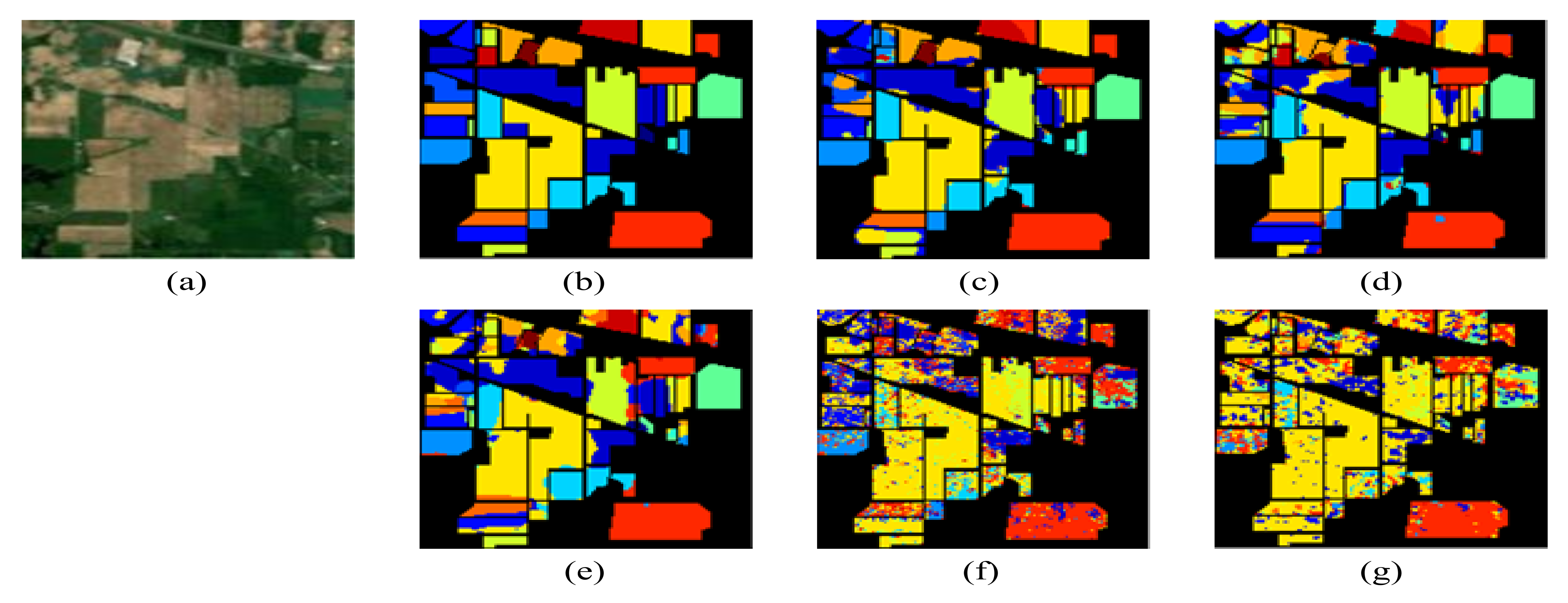
3.5.1. Test Results on Indian Pines Dataset

From 220 bands of the IP scene dataset, 15 × 15 × 16 (S × S × B) data blocks were extracted to calculate the original spectral–spatial features and used as the input to the network, where the window size, S = 15, the number of bands after the dimensionality reduction by PCA, B = 16, and the optimal band selection ratio λ = 0.10 is selected for the best OA performance as shown in Table 2. With respect to average accuracy (AA), OA, and Kappa evaluation metrics, the proposed methods are not superior to other methods. This could be due to the small size of the dataset which contains 145 × 145 pixels. However, in comparison with other methods, the processing time of the proposed methods C-CNN and C-CNN-Aug is the best. The visual results of HSI classification by the five methods are shown in Figure 7. The performance comparison is shown in Table 4.

3.5.2. Test Results on Pavia University Dataset

With 103 bands of the PU scene dataset, 15 × 15 × 8 (S × S × B) data blocks have been extracted to calculate the original spectral–spatial features and used as the input to the network, where the window size, S = 15, the number of bands after the dimensionality reduction by PCA, B = 8, and the optimal band selection ratio λ = 0.08 is selected for the best OA performance as shown in Table 2. Our proposed method has surpassed the other methods in terms of AA, OA, Kappa, and processing time. In comparison with other methods, the OA performance of the proposed method C-CNN is 97.08%. On the other hand, the C-CNN-Aug has achieved OA of 98.25% which is comparable to DSSIRNet method. Nevertheless, the running time of the proposed methods reached 79 s, which is faster than that of the other methods. The maps of hyperspectral images classification by the five methods are shown in Figure 8. The performance comparison is presented in Table 5.

3.5.3. Test Results on Salinas Scene Dataset

With SA scene dataset (including 224 bands), the 15 × 15 × 20 (S × S × B) data blocks are extracted to calculate the original spectral–spatial features and used as the input to the proposed network, where the window size, S = 15, the number of bands after the dimensionality reduction by PCA, B = 20, and the optimal band selection ratio λ = 0.10. The OA of the proposed C-CNN-Aug on the SA map dataset is higher than those of other methods. Additionally, better performance is achieved in terms of the processing time, where the proposed methods achieved 196 seconds of processing time. The classification maps obtained by SS-3DCNN, SSAF-DCR, DSSIRNet, C-CNN, and C-CNN-Aug are shown in Figure 9. The comparison results are shown in Table 6.

3.6. The Impact of Training Sample Ratio on Overall Accuracy

The effectiveness of the proposed models on various training sample ratios has been evaluated and demonstrated in this Section 1%, 2%, 3%, 4%, and 5% of the labeled training samples from each class have been used to form the training sets, and then evaluated the performance of different methods on the benchmark datasets. The Figure 10 shows the OA results on different training samples ratios of IP, PU, and SA datasets, respectively. It can be clearly seen that the proposed C-CNN and C-CNN-Aug achieve better OA than other methods on PU and SA especially when the ratio of the training sample increases. On the other hand, the proposed C-CNN and C-CNN-Aug performed worse than the other methods on the IP dataset. However, the processing time of C-CNN and C-CNN-Aug is better than other methods on IP dataset as well as the other two datasets, PU and SA.

3.7. The Impact of Multi-GPUs Implementation with NVLink on Processing Time

To further improve the performance, another experimental environment was set to evaluate the influence of the NVLink [48] on the processing time. In hardware, we increased the number of GPUs (GeForce RTX 2080 Ti) from 1 to 2 by the NIVIDA NVLink technology for GPU interconnection. For building the extra software for the evaluation environment, we firstly set up Docker 18.06.1-ce, then, installed NVIDIA Container Toolkit and NVIDIA NGC to support NVIDIA SLI technology, which is able to merge and utilize multi-GPUs’ capability efficiently. The container image employed is the nvcr.io/nvidia/tensorflow: 18.04-py3 linked with NCCL and CUDA 9.0. The processing time with the benchmark datasets is shown in Table 7. The observations indicate that the implementation of HPC by employing the NVLink technology with 2xGPU is a significant advance that makes the training phase of deep neural network more efficient.

4. Discussion

In deep neural network (DNN) models such as CNN are prone to overfitting because of the large number of parameters and the small amount of training data used to train the model. Consequently, the model is able to perform well on the training samples, but its results on the validation or testing samples are poor. Therefore, the model cannot be generalized to new data samples. This issue of overfitting can be worse in the field of remote sensing due to the complexity of data such as hyperspectral images which are composed of thousands of spectral channels. Typically, techniques such as data augmenting, Dropout regularization, and L1/L2 regularization are used to reduce the impact of such an issue. The vanishing gradient is another issue faced by deep CNN models. The vanishing gradient problem arises from the backpropagation technique used for updating the DNN models’ parameters during the training process. For example, in the gradient descent algorithm, the gradient might fade slightly as it passes through each layer of the CNN, resulting in its disappearance or vanishing. To avoid this problem, an appropriate learning rate should be used, making the gradient to perform appropriate steps until convergence. However, finding the optimal learning rate is another issue. To address such an issue, an adaptive variant of optimizers such as adaptive moment estimation (Adam) was proposed. In comparison to other optimizers, the superiority of Adam optimizer for HSI classification was demonstrated in [49]. The main goal of the proposed C-CNN method is to achieve satisfactory HSI classification accuracy while accelerate the computing processes and provide faster response time for the HSI classification. Hence, several techniques have been implemented and incorporated into the proposed method in order to achieve this goal. These techniques include principal component analysis (PCA), image augmentation, Dropout, and L2 regularization. Moreover, the impact of band selection ratio, window size, training sample ratio, and multi-GPUs on the model performance was evaluated. The implementation of C-CNN without the PCA led to similar results as those of the λ = 0.01. Hence, only the results of the C-CNN with PCA were discussed in the paper. The spectral bands have been intentionally reduced by a small ratio of λ ranging from 0.01 to 0.10 to preserve as much useful information as possible and keep the computational cost low. More importantly, this small ratio of λ can mitigate any potential negative impact of PCA on the spectral data while providing comparable performance. The appropriate λ value is determined by both the OA and computational complexity. For example, for the IP and PU datasets, the optimal OA is λ = 0.10 and λ = 0.08, respectively. For the SA dataset, the OA reached to 99% at λ = 0.03, and continued rising up to 99.43% at λ = 0.10. On the other hand, the optimal processing time is reached when λ = 0.10. Image augmentation methods including rotation and flipping have been applied to increase the number of training samples and reduce the impact of overfitting. The impact of image augmentation methods on the performance of the proposed method is shown in Table 4, Table 5 and Table 6. The most noticeable improvement is shown in Table 4, where the proposed C-CNN with image augmentation (C-CNN-Aug) has yielded to ∼15% improvement in terms of AA, OA, and Kappa on Indian Pines dataset. Dropout and L2 regularization techniques were adopted to further reduce the model complexity and prevent overfitting. Additionally, the 15 × 15 was finally decided in this study as it turns out that the 15 × 15 window size offers the best trade-off between the OA and testing time as shown in Table 3. The impact of several training sample ratios on the proposed model is shown in Figure 10, where the OA of the proposed C-CNN and C-CNN-Aug increases on Indian Pines, Pavia University, and Salinas Scene dataset when the ratio of the training sample increases. Finally, by using multi-GPUs with 2xNVIDIA GeForce RTX 2080 Ti, NVLink, the processing time has been improved by ∼44% with the three standard datasets.

5. Conclusions

This study proposed a convolutional neural network called consolidated convolutional neural network (C-CNN) by combining a 3D-CNN and a 2D-CNN for better and faster hyperspectral image (HSI) classification than those of the previous state-of-the-art methods. The experimental results on the benchmark datasets of Indian Pines (IP), Pavia University (PU), and Salinas Scene (SA) proved that our proposed C-CNN and the augmented C-CNN (C-CNN-Aug) methods can firmly reduce the complexity of the model, and effectively resolve the overfitting problem by applying deep learning techniques such as image augmentation, Dropout, and L2 regularization. Moreover, principal component analysis (PCA) has been used to reduce the spectral bands dimensionality of the input HSIs. Consequently, the accuracy and the processing time have been significantly improved on most of the benchmark datasets. Furthermore, the impact of PCA band selection ratio λ and window size on the overall accuracy (OA) were presented. The OA of the proposed model reached 83.68%, 98.25%, and 99.43% on IP, PU, and SA datasets, respectively. By enhancing the computing power with 2xNVIDIA GeForce RTX 2080 Ti, NVLink, the processing time has been further improved by ∼44%. Future work will study the effectiveness of varying the PCA band selection ratio λ on the processing time. Additionally, the impact of the variation of the data size on the classification results will be investigated.

Author Contributions

Conceptualization, Y.-L.C., T.-H.T., K.-C.F. and W.-H.L.; methodology, Y.-L.C., M.A., L.C. and T.-H.T.; software, W.-H.L.; validation, M.A., Y.-N.C. and Y.-L.C.; formal analysis, Y.-L.C. and M.A.; investigation, W.-H.L. and M.A.; data curation, W.-H.L.; writing—review and editing, W.-H.L., M.A. and Y.-L.C.; supervision, Y.-L.C. and M.A. All authors have read and agreed to the published version of the manuscript.

Funding

This work was funded by the Ministry of Science and Technology, Taiwan, Grant No. MOST 110-2622-E-027-025, 110-2119-M-027-001, 110-2221-E-027-101, 109-2116-M-027-004; and National Space Organization, Grant No. NSPO-S-110244; and National Science and Technology Center for Disaster Reduction, Grant No. NCDR-S-110096.

Institutional Review Board Statement

Not applicable.

Informed Consent Statement

Not applicable.

Data Availability Statement

The Indiana Pines, University of Pavia, and Salinas Valley datasets are available online at http://www.ehu.eus/ccwintco/index.php?title=Hyperspectral_Remote_Sensing_Scenes, (accessed on 16 February 2022).

Conflicts of Interest

The authors declare no conflict of interest.

References

  1. Guo, A.; Huang, W.; Dong, Y.; Ye, H.; Ma, H.; Liu, B.; Wu, W.; Ren, Y.; Ruan, C.; Geng, Y. Wheat yellow rust detection using UAV-based hyperspectral technology. Remote Sens. 2021, 13, 123. [Google Scholar] [CrossRef]
  2. Liu, N.; Townsend, P.A.; Naber, M.R.; Bethke, P.C.; Hills, W.B.; Wang, Y. Hyperspectral imagery to monitor crop nutrient status within and across growing seasons. Remote Sens. Environ. 2021, 255, 112303. [Google Scholar] [CrossRef]
  3. Lyu, X.; Li, X.; Dang, D.; Dou, H.; Xuan, X.; Liu, S.; Li, M.; Gong, J. A new method for grassland degradation monitoring by vegetation species composition using hyperspectral remote sensing. Ecol. Indic. 2020, 114, 106310. [Google Scholar] [CrossRef]
  4. Marinelli, D.; Bovolo, F.; Bruzzone, L. A novel change detection method for multitemporal hyperspectral images based on binary hyperspectral change vectors. IEEE Trans. Geosci. Remote Sens. 2019, 57, 4913–4928. [Google Scholar] [CrossRef]
  5. Hou, Z.; Li, W.; Li, L.; Tao, R.; Du, Q. Hyperspectral change detection based on multiple morphological profiles. IEEE Trans. Geosci. Remote Sens. 2021, 60, 5507312. [Google Scholar] [CrossRef]
  6. Huang, P.; Guo, Q.; Han, C.; Zhang, C.; Yang, T.; Huang, S. An Improved Method Combining ANN and 1D-Var for the Retrieval of Atmospheric Temperature Profiles from FY-4A/GIIRS Hyperspectral Data. Remote Sens. 2021, 13, 481. [Google Scholar] [CrossRef]
  7. Calin, M.A.; Calin, A.C.; Nicolae, D.N. Application of airborne and spaceborne hyperspectral imaging techniques for atmospheric research: Past, present, and future. Appl. Spectrosc. Rev. 2021, 56, 289–323. [Google Scholar] [CrossRef]
  8. Paoletti, M.E.; Haut, J.M.; Pereira, N.S.; Plaza, J.; Plaza, A. Ghostnet for hyperspectral image classification. IEEE Trans. Geosci. Remote Sens. 2021, 59, 10378–10393. [Google Scholar] [CrossRef]
  9. Zhao, B.; Ulfarsson, M.O.; Sveinsson, J.R.; Chanussot, J. Unsupervised and supervised feature extraction methods for hyperspectral images based on mixtures of factor analyzers. Remote Sens. 2020, 12, 1179. [Google Scholar] [CrossRef] [Green Version]
  10. Paoletti, M.E.; Haut, J.M.; Tao, X.; Miguel, J.P.; Plaza, A. A new GPU implementation of support vector machines for fast hyperspectral image classification. Remote Sens. 2020, 12, 1257. [Google Scholar] [CrossRef] [Green Version]
  11. Cao, F.; Yang, Z.; Ren, J.; Ling, W.K.; Zhao, H.; Sun, M.; Benediktsson, J.A. Sparse representation-based augmented multinomial logistic extreme learning machine with weighted composite features for spectral—Spatial classification of hyperspectral images. IEEE Trans. Geosci. Remote Sens. 2018, 56, 6263–6279. [Google Scholar] [CrossRef] [Green Version]
  12. Jiang, J.; Ma, J.; Chen, C.; Wang, Z.; Cai, Z.; Wang, L. SuperPCA: A superpixelwise PCA approach for unsupervised feature extraction of hyperspectral imagery. IEEE Trans. Geosci. Remote Sens. 2018, 56, 4581–4593. [Google Scholar] [CrossRef] [Green Version]
  13. Li, X.; Zhang, L.; You, J. Hyperspectral image classification based on two-stage subspace projection. Remote Sens. 2018, 10, 1565. [Google Scholar] [CrossRef] [Green Version]
  14. Yu, H.; Xu, Z.; Wang, Y.; Jiao, T.; Guo, Q. The use of KPCA over subspaces for cross-scale superpixel based hyperspectral image classification. Remote Sens. Lett. 2021, 12, 470–477. [Google Scholar] [CrossRef]
  15. Uddin, M.P.; Mamun, M.A.; Afjal, M.I.; Hossain, M.A. Information-theoretic feature selection with segmentation-based folded principal component analysis (PCA) for hyperspectral image classification. Int. J. Remote Sens. 2021, 42, 286–321. [Google Scholar] [CrossRef]
  16. Seifi Majdar, R.; Ghassemian, H. A probabilistic SVM approach for hyperspectral image classification using spectral and texture features. Int. J. Remote Sens. 2017, 38, 4265–4284. [Google Scholar] [CrossRef]
  17. Zhang, Y.; Cao, G.; Li, X.; Wang, B.; Fu, P. Active semi-supervised random forest for hyperspectral image classification. Remote Sens. 2019, 11, 2974. [Google Scholar] [CrossRef] [Green Version]
  18. Wang, X. Kronecker Factorization-Based Multinomial Logistic Regression for Hyperspectral Image Classification. IEEE Geosci. Remote Sens. Lett. 2021, 19, 1–5. [Google Scholar] [CrossRef]
  19. Ma, L.; Crawford, M.M.; Tian, J. Local manifold learning-based k-nearest-neighbor for hyperspectral image classification. IEEE Trans. Geosci. Remote Sens. 2010, 48, 4099–4109. [Google Scholar] [CrossRef]
  20. Wei, W.; Ma, M.; Wang, C.; Zhang, L.; Zhang, P.; Zhang, Y. A novel analysis dictionary learning model based hyperspectral image classification method. Remote Sens. 2019, 11, 397. [Google Scholar] [CrossRef] [Green Version]
  21. Khotimah, W.N.; Bennamoun, M.; Boussaid, F.; Sohel, F.; Edwards, D. A high-performance spectral-spatial residual network for hyperspectral image classification with small training data. Remote Sens. 2020, 12, 3137. [Google Scholar] [CrossRef]
  22. Ge, Z.; Cao, G.; Li, X.; Fu, P. Hyperspectral image classification method based on 2D–3D CNN and multibranch feature fusion. IEEE J. Sel. Top. Appl. Earth Obs. Remote Sens. 2020, 13, 5776–5788. [Google Scholar] [CrossRef]
  23. Zheng, J.; Feng, Y.; Bai, C.; Zhang, J. Hyperspectral image classification using mixed convolutions and covariance pooling. IEEE Trans. Geosci. Remote Sens. 2020, 59, 522–534. [Google Scholar] [CrossRef]
  24. Feng, Y.; Zheng, J.; Qin, M.; Bai, C.; Zhang, J. 3D Octave and 2D Vanilla Mixed Convolutional Neural Network for Hyperspectral Image Classification with Limited Samples. Remote Sens. 2021, 13, 4407. [Google Scholar] [CrossRef]
  25. Farooque, G.; Xiao, L.; Yang, J.; Sargano, A.B. Hyperspectral Image Classification via a Novel Spectral–Spatial 3D ConvLSTM-CNN. Remote Sens. 2021, 13, 4348. [Google Scholar] [CrossRef]
  26. Jiang, Y.; Li, Y.; Zou, S.; Zhang, H.; Bai, Y. Hyperspectral image classification with spatial consistence using fully convolutional spatial propagation network. IEEE Trans. Geosci. Remote Sens. 2021, 59, 10425–10437. [Google Scholar] [CrossRef]
  27. Zhang, D.; Shao, J.; Li, X.; Shen, H.T. Remote sensing image super-resolution via mixed high-order attention network. IEEE Trans. Geosci. Remote Sens. 2020, 59, 5183–5196. [Google Scholar] [CrossRef]
  28. LeCun, Y.; Bengio, Y.; Hinton, G. Deep learning. Nature 2015, 521, 436–444. [Google Scholar] [CrossRef]
  29. Maxwell, A.E.; Warner, T.A.; Fang, F. Implementation of machine-learning classification in remote sensing: An applied review. Int. J. Remote Sens. 2018, 39, 2784–2817. [Google Scholar] [CrossRef] [Green Version]
  30. Ma, L.; Liu, Y.; Zhang, X.; Ye, Y.; Yin, G.; Johnson, B.A. Deep learning in remote sensing applications: A meta-analysis and review. ISPRS J. Photogramm. Remote Sens. 2019, 152, 166–177. [Google Scholar] [CrossRef]
  31. Li, S.; Song, W.; Fang, L.; Chen, Y.; Ghamisi, P.; Benediktsson, J.A. Deep learning for hyperspectral image classification: An overview. IEEE Trans. Geosci. Remote Sens. 2019, 57, 6690–6709. [Google Scholar] [CrossRef] [Green Version]
  32. Meng, Z.; Li, L.; Jiao, L.; Feng, Z.; Tang, X.; Liang, M. Fully dense multiscale fusion network for hyperspectral image classification. Remote Sens. 2019, 11, 2718. [Google Scholar] [CrossRef] [Green Version]
  33. Feng, J.; Wu, X.; Shang, R.; Sui, C.; Li, J.; Jiao, L.; Zhang, X. Attention multibranch convolutional neural network for hyperspectral image classification based on adaptive region search. IEEE Trans. Geosci. Remote Sens. 2020, 59, 5054–5070. [Google Scholar] [CrossRef]
  34. Paoletti, M.E.; Haut, J.M.; Plaza, J.; Plaza, A. Deep&dense convolutional neural network for hyperspectral image classification. Remote Sens. 2018, 10, 1454. [Google Scholar]
  35. Acquarelli, J.; Marchiori, E.; Buydens, L.; Tran, T.; van Laarhoven, T. Convolutional neural networks and data augmentation for spectral-spatial classification of hyperspectral images. Networks 2017, 16, 21–40. [Google Scholar]
  36. Srivastava, N.; Hinton, G.; Krizhevsky, A.; Sutskever, I.; Salakhutdinov, R. Dropout: A simple way to prevent neural networks from overfitting. J. Mach. Learn. Res. 2014, 15, 1929–1958. [Google Scholar]
  37. Yu, C.; Han, R.; Song, M.; Liu, C.; Chang, C.I. A simplified 2D-3D CNN architecture for hyperspectral image classification based on spatial–spectral fusion. IEEE J. Sel. Top. Appl. Earth Obs. Remote Sens. 2020, 13, 2485–2501. [Google Scholar] [CrossRef]
  38. Xu, Q.; Xiao, Y.; Wang, D.; Luo, B. CSA-MSO3DCNN: Multiscale octave 3D CNN with channel and spatial attention for hyperspectral image classification. Remote Sens. 2020, 12, 188. [Google Scholar] [CrossRef] [Green Version]
  39. Yang, X.; Ye, Y.; Li, X.; Lau, R.Y.; Zhang, X.; Huang, X. Hyperspectral image classification with deep learning models. IEEE Trans. Geosci. Remote Sens. 2018, 56, 5408–5423. [Google Scholar] [CrossRef]
  40. Sellami, A.; Farah, M.; Farah, I.R.; Solaiman, B. Hyperspectral imagery classification based on semi-supervised 3-D deep neural network and adaptive band selection. Expert Syst. Appl. 2019, 129, 246–259. [Google Scholar] [CrossRef]
  41. Zhang, T.; Shi, C.; Liao, D.; Wang, L. A Spectral Spatial Attention Fusion with Deformable Convolutional Residual Network for Hyperspectral Image Classification. Remote Sens. 2021, 13, 3590. [Google Scholar] [CrossRef]
  42. Zhang, T.; Shi, C.; Liao, D.; Wang, L. Deep Spectral Spatial Inverted Residual Network for Hyperspectral Image Classification. Remote Sens. 2021, 13, 4472. [Google Scholar] [CrossRef]
  43. Chen, Y.; Jiang, H.; Li, C.; Jia, X.; Ghamisi, P. Deep feature extraction and classification of hyperspectral images based on convolutional neural networks. IEEE Trans. Geosci. Remote Sens. 2016, 54, 6232–6251. [Google Scholar] [CrossRef] [Green Version]
  44. Nair, V.; Hinton, G.E. Rectified linear units improve restricted boltzmann machines. In Proceedings of the 27th International Conference on International Conference on Machine Learning (ICML), Haifa, Israel, 21–24 June 2010; pp. 807–814. [Google Scholar]
  45. Cortes, C.; Mohri, M.; Rostamizadeh, A. L2 regularization for learning kernels. arXiv 2012, arXiv:1205.2653. [Google Scholar]
  46. Hinton, G.E.; Srivastava, N.; Krizhevsky, A.; Sutskever, I.; Salakhutdinov, R.R. Improving neural networks by preventing co-adaptation of feature detectors. arXiv 2012, arXiv:1207.0580. [Google Scholar]
  47. Kingma, D.P.; Ba, J. Adam: A method for stochastic optimization. arXiv 2014, arXiv:1412.6980. [Google Scholar]
  48. Li, A.; Song, S.L.; Chen, J.; Li, J.; Liu, X.; Tallent, N.R.; Barker, K.J. Evaluating modern gpu interconnect: Pcie, nvlink, nv-sli, nvswitch and gpudirect. IEEE Trans. Parallel Distrib. Syst. 2019, 31, 94–110. [Google Scholar] [CrossRef] [Green Version]
  49. Bera, S.; Shrivastava, V.K. Analysis of various optimizers on deep convolutional neural network model in the application of hyperspectral remote sensing image classification. Int. J. Remote Sens. 2020, 41, 2664–2683. [Google Scholar] [CrossRef]
Figure 1. The proposed C-CNN model architecture.
Remotesensing 14 01571 g001
Figure 2. C-CNN training and testing flow chart.
Remotesensing 14 01571 g002
Figure 3. Land cover category of Indian Pines dataset.
Remotesensing 14 01571 g003
Figure 4. Land cover category of Pavia University dataset.
Remotesensing 14 01571 g004
Figure 5. Land cover category of Salinas Scene dataset.
Remotesensing 14 01571 g005
Figure 6. The effect of different window size on the overall accuracy of C-CNN-Aug.
Remotesensing 14 01571 g006
Figure 7. (a) False-color composite (R: 26, G: 14, B: 8), (b) ground truth, (c) SS-3DCNN (97.89%), (d) SSAF-DCR (96.36%), (e) DSSIRNet (97.18%), (f) C-CNN (73.33%), (g) C-CNN-Aug (83.68%).
Remotesensing 14 01571 g007
Figure 8. (a) False-color composite (R: 53, G: 31, B: 8), (b) Ground truth, (c) SS-3DCNN (98.45%), (d) SSAF-DCR (97.43%), (e) DSSIRNet (99.31%), (f) C-CNN (97.08%), (g) C-CNN-Aug (98.25%).
Remotesensing 14 01571 g008
Figure 9. (a) False-color composite (R: 53, G: 31, B: 8), (b) Ground truth, (c) SS-3DCNN (98.29%), (d) SSAF-DCR (96.53%), (e) DSSIRNet (99.35%), (f) C-CNN (99.22%), (g) C-CNN-Aug (99.43%).
Remotesensing 14 01571 g009
Figure 10. The overall accuracy performance comparison for different sample ratio of datasets and methods.
Remotesensing 14 01571 g010
Table 1. Indian Pines, Pavia University, and Salinas Scene datasets information.
Data SetPixelsSpatial ResolutionBandsWavelength RangeDiscarded BandsClasses
Indian Pines 145 × 145 20 m/pixel224400∼2400 nm2416
Pavia University 610 × 340 1.3 m/pixel103430∼860 nm09
Salinas Scene 512 × 217 3.7 m/pixel224360∼2500 nm2016
Table 2. The impact of band selection ratio λ on the overall accuracy (OA) of C-CNN-Aug.
λ IPPUSA
0.0165.0894.2395.79
0.0277.5595.8898.21
0.0380.4296.6299.00
0.0480.4996.6499.08
0.0581.3297.6899.06
0.0682.2498.0099.28
0.0782.2897.9399.25
0.0883.5798.2599.28
0.0983.5398.1999.36
0.1083.6898.2099.43
Table 3. The impact of window size on the overall accuracy and testing time of C-CNN-Aug, where λ   =   0.10 .
Window SizeOverall Accuracy (OA)Time (Seconds)
IPPUSAIPPUSA
5 × 5 70.2695.4696.24103754
15 × 1583.6898.2099.433995196
25 × 25 84.2898.8799.6797210486
35 × 35 84.0998.7799.80185395953
Herein, λ is defined as the band selection ratio.
Table 4. The accuracy comparison of Indian Pines classification.
ClassSS-3DCNN [40]SSAF-DCR [41]DSSIRNet [42]C-CNNC-CNN-Aug
197.9697.8298.8842.0061.93
296.4996.0396.6558.1575.82
399.5396.3996.6454.2775.75
497.4796.0094.8118.3448.47
597.2199.5198.6280.9081.69
695.2499.0999.1392.9994.75
798.8871.1394.1870.0089.29
898.51100.099.9298.4699.32
997.7396.9083.7176.5079.83
1094.4493.1197.0767.6779.50
1197.8397.1497.6583.0688.41
1297.7093.5898.6945.3867.12
1397.2499.69100.076.0696.49
1496.4797.0598.7895.6995.46
1595.8195.1395.7654.2771.68
1699.8397.6398.7059.2491.85
AA97.3995.3996.8267.0681.08
OA97.8996.3697.1873.3383.68
Kappa98.7295.8596.7869.4381.25
Time (s)37147403939
Table 5. The accuracy comparison of Pavia University classification.
ClassSS-3DCNN [40]SSAF-DCR [41]DSSIRNet [42]C-CNNC-CNN-Aug
198.0198.8099.0497.6398.64
299.41100.0100.099.7599.74
398.9294.4698.7083.7492.50
498.1599.1697.9894.6294.89
598.20100.0100.099.7399.91
699.3197.95100.098.6899.11
798.0894.1199.3995.3198.04
898.0688.2397.8691.4695.26
999.23100.099.8990.2194.68
AA98.6096.9699.2094.5796.98
OA98.4597.4399.3197.0898.25
Kappa98.530.9799.0596.1397.68
Time (s)2651561007979
Table 6. The accuracy comparison of Salinas Scene classification.
ClassSS-3DCNN [40]SSAF-DCR [41]DSSIRNet [42]C-CNNC-CNN-Aug
196.73100.0100.099.9499.91
298.5099.93100.099.6399.99
396.0698.3399.8699.8099.83
498.8096.9999.6699.4998.89
597.8897.6899.9199.0899.07
698.87100.0100.099.9499.93
796.58100.0100.099.9699.97
898.6192.7299.0798.3999.22
998.9299.86100.0100.099.99
1098.3098.6499.7997.9298.23
1198.9696.9197.7899.9499.87
1299.7197.43100.099.9399.61
1398.7896.7899.8099.1599.24
1498.9699.2798.9398.9098.81
1598.0191.4998.8398.8799.00
1698.77100.0100.099.2999.35
AA98.2897.8799.6099.3999.43
OA98.2996.5399.3599.2299.43
Kappa98.1696.1499.2799.1399.36
Time (s)289198219196196
Table 7. The processing time comparison by 1 and 2 GPUs on benchmark datasets (Measured unit: Second).
DatasetC-CNN-Aug, 1 × 2080TiC-CNN-Aug, 2 × 2080TiImproved%
IP321844
PU794543
SA19711144
Publisher’s Note: MDPI stays neutral with regard to jurisdictional claims in published maps and institutional affiliations.

