Article

Unsupervised Remote Sensing Image Super-Resolution Guided by Visible Images

School of Electronic Information and Communications, Huazhong University of Science and Technology, Wuhan 430074, China
*
Author to whom correspondence should be addressed.
Remote Sens. 2022, 14(6), 1513; https://doi.org/10.3390/rs14061513
Submission received: 22 February 2022 / Revised: 18 March 2022 / Accepted: 18 March 2022 / Published: 21 March 2022
(This article belongs to the Special Issue Advanced Super-resolution Methods in Remote Sensing)

Abstract

:
Remote sensing images are widely used in many applications. However, due to being limited by the sensors, it is difficult to obtain high-resolution (HR) images from remote sensing images. In this paper, we propose a novel unsupervised cross-domain super-resolution method devoted to reconstructing a low-resolution (LR) remote sensing image guided by an unpaired HR visible natural image. Therefore, an unsupervised visible image-guided remote sensing image super-resolution network (UVRSR) is built. The network is divided into two learnable branches: a visible image-guided branch (VIG) and a remote sensing image-guided branch (RIG). As HR visible images can provide rich textures and sufficient high-frequency information, the purpose of VIG is to treat them as targets and make full use of their advantages in reconstruction. Specially, we first use a CycleGAN to drag the LR visible natural images to the remote sensing domain; then, we apply an SR network to upscale these simulated remote sensing domain LR images. However, the domain gap between SR remote sensing images and HR visible targets is massive. To enforce domain consistency, we propose a novel domain-ruled discriminator in the reconstruction. Furthermore, inspired by the zero-shot super-resolution network (ZSSR) to explore the internal information of remote sensing images, we add a remote sensing domain inner study to train the SR network in RIG. Sufficient experimental works show UVRSR can achieve superior results with state-of-the-art unpaired and remote sensing SR methods on several challenging remote sensing image datasets.

1. Introduction

Remote sensing images are currently being used in many applications, such as weather alerts [1], land cover classification [2,3], and target detection [4,5,6]. In fact, high-resolution (HR) remote sensing images are required in these applications for precise prediction. While visible images have rich textures and detailed content in their HR images, the visual resolution of most remote sensing images is poor and limited by various sensors in satellites due to their high altitude. Moreover, monsoons, clouds, and detector blur and noise can also degrade the quality of remote sensing images. Consequently, it is difficult to obtain high-quality satellite images, and this undoubtedly will constrain their further applications. One cost-efficient technique to increase the spatial resolution of remotely sensed data is image super-resolution (SR).
Image SR is an important issue in image processing tasks. It can be defined as a key preprocessing stage for image identification, image classification, and image segmentation, etc. The purpose of SR is to scale up a single degraded low-resolution (LR) image to a corresponding HR image in software without having to update the hardware, thereby keeping hardware costs in hand, especially considering the scaling factor up to 8 × (8 times). Nonetheless, SR incurs two challenges: the high number of potential super-resolution results from the corresponding LR, and the difficulty in defining a model to produce an optimal SR result. With the evolution of deep learning methods and models, SR research is rapidly improving. Deep learning SR models have demonstrated the capability to identify likely HR reconstructions by capturing detailed prior information about images. These methods have achieved remarkable performance by leveraging convolutional neural networks (CNNs) [7,8,9,10,11,12,13] and generative adversarial networks (GANs) [14,15,16,17,18].
All existing SR models can be classified into two kinds of techniques, supervised or unsupervised SR, depending on the training data. Most models are trained in a supervised manner, in that indispensable HR/LR image pairs should be provided in the model training. Essential HR image datasets including visible clean datasets, such as DIV2K [19], SET5 [20], URBAN [21], and B100 [22], are adopted to generate paired HR/LR training data by downsampling the HR images. Regarding the unsupervised category, these SR approaches estimate the HR information in the result with the LR input image itself. This is because in most practical applications, including remote sensing images, infrared images, real-world visible images, and HR datasets are always unavailable. Recently, some work [23,24,25,26] has adopted unpaired training in unsupervised SR. Specifically, they built the models to enhance the resolution of LR data by other HR image datasets and trained the model with these unpaired HR/LR counterparts.
Real-world visible image SR [25,26,27,28,29,30,31] deals with unpaired training. Real-world images are captured by various visible sensors such as cameras, smartphones, and surveillance cameras, but it can be arduous to obtain HR/LR pairs due to the shaking of sensors or changing backgrounds. Recently, CycleGAN [32] was proposed to translate an image from a source domain to a target domain in the absence of training paired examples. Some recent work applied CycleGAN to real-world SR. Bulat et al. [26] first applied CycleGAN to real-world facial SR. Specifically, guided by an unpaired LR real-world face, they exploited CycleGAN to transfer a LR clean facial image to the real-world domain. Then, a stacked SR network after CycleGAN scaled up the resolution of this LR simulated real-world face to the expected scale. In their pipeline, they trained CycleGAN and the SR network together with several loss functions. Yuan et al. [31] improved Bulat’s model and used a cycle-in-cycle network in natural real-world image SR. Their work used two CycleGANs, one to learn real-world degradation similar to Butal et al. [26], and the next to perform the SR task. To maintain the content consistency, an additional CycleGAN was used to ensure that the final result can go back to the initial input. However, the recent work on the zero-shot super-resolution network (ZSSR) [33] offered another way of performing unsupervised SR. They first trained paired HR/LR synthetic image pairs in a single SR network and downsampled the LR real image to an expected scale. Then, they applied these downsampled LR real image/LR real image pairs to continue to train the SR network in a test time, which can also be regarded as online training. This training strategy can be used to explore the inner relationship of real-world images. In this paper, we take full advantage of both CycleGAN and ZSSR in our unsupervised remote sensing SR model.
In remote sensing scenarios, to the best of our knowledge, there is very limited work on the training setting of unpaired HR/LR images. Most remote sensing SR methods [34,35,36,37,38] simply treat the initial remote sensing image from the dataset and its downsampled counterpart as HR/LR. However, there are two key problems in this setting. Because the resolution of the initial remote sensing image is low and lacks details, it is improper to treat it as the target. In addition, the degradation between HR/LR remote sensing is unknown and more complicated than when it is simply downsampled. To deal with an unpaired setting, Haut et al. [39] proposed an unsupervised learning model for generating remote sensing images from unpaired random noise and improved the resolution of remote sensing imagery. Later, Wang et al. [40] improved this noise generation strategy. In their implementation, they encoded the reference image into the latent space as the migration image prior and updated noise maps to obtain a more stable and detailed reconstruction. However, noise itself has meaningful high-frequency information; this constrains the further improvement of remote sensing images.
Rather than random noise, visible HR clean images have more meaningful textures and can provide sufficient high-frequent information. In this paper, we use HR clean images as a target to guide remote sensing SR. Nonetheless, the domain distance between the visible clean images and remote sensing images is much greater than that between the visible clean images and the real-world images, and the direct use of the models in real-world SR is more likely to cause domain shift in the reconstruction. How to explore the ability of an HR clean target in the reconstruction without domain shift is a significant challenge in remote sensing SR.
To resolve this problem, we proposed a novel unsupervised GAN-based and cross-domain super-resolution network for remote sensing images, which we call UVRSR. The network is divided into two learnable branches: the visible image guide branch (VIG) and the remote sensing image guide branch (RIG). The design of the VIG is to explore the high frequency information and textures in HR clean images for the network. To avoid domain shift in the reconstruction, we design a novel domain-ruled(DR) discriminator to ensure domain consistency. The DR discriminator learns to determine the remote sensing domain by remote sensing the target, and it learns to determine the content by the HR visible target. Moreover, it enhances the target domain to avoid domain shift in the reconstruction. In addition, to learn the remote sensing inner relationship, we add a RIG to the SR network.
In summary, our contributions are:
  • To the best of our knowledge, this is the first work to perform cross-domain SR in the absence of HR/LR image pairs, as well as the first to apply visible images to assist in remote sensing domain image SR;
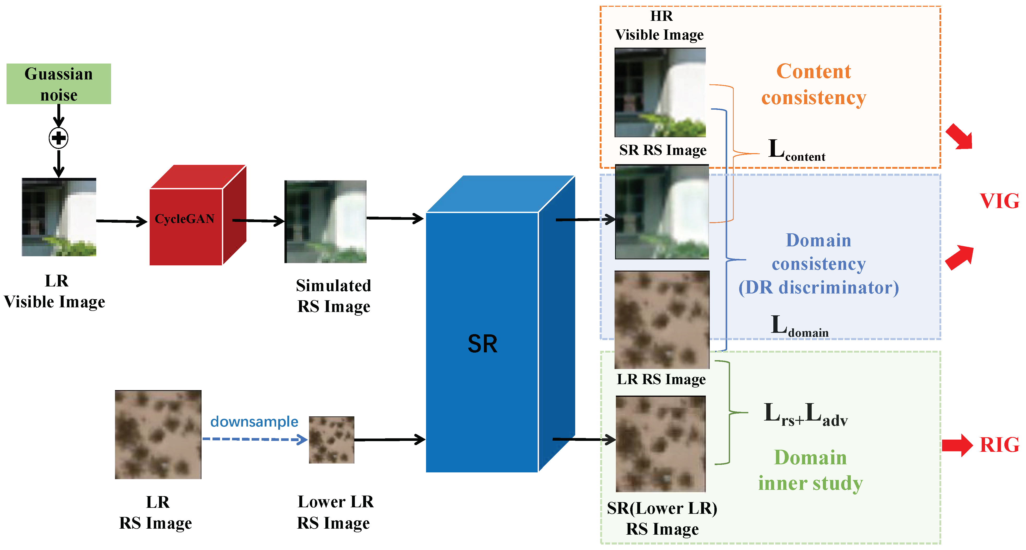
  • This paper proposes a novel two-branch network, UVRSR, to produce an SR remote sensing domain image with an HR visible image and an unpaired LR remote sensing image. A CycleGAN-based learnable branch VIG is proposed to dig the rich textures from HR visible images, and another learnable branch, RIG, is built to explore the internal information of remote sensing images;
  • We design a novel domain-ruled (DR) discriminator to determine the SR output to the target remote sensing domain without domain shift in the reconstruction;
  • Experiments show that UVRSR can achieve superior results when compared with state-of-the-art unpaired and remote sensing SR methods on the remote sensing UC Merced and the NWPU-RESISC45 datasets.
The paper is organized as follows. Section 2 investigates work related to our proposed method. Section 3 describes the theory, structure and training of our proposed UVRSR model. Section 4 illustrates our experimental work and analysis in multiple remote sensing datasets. Section 5 further discusses the effects of our proposed model. Section 6 contains our conclusions and future work indications.

2. Related Work

2.1. Remote Sensing Super-Resolution

The first work on remote sensing SR was proposed by Tsai et al. [41]. These authors applied frequency-domain to upscale LR images by multiple downsampled images. Then, with the proposal of various image processing techniques, including domain wavelet transformation (DWT), maximum a posterior (MAP), total variation (TV), iterative back-projection (IBP) and projection onto convex sets (POCS), in the following years, remote sensing SR rapidly developed. Tao et al. [42] first applied the DWT method in remote sensing SR. The SR result is obtained by the inverse discrete wavelet transform. Wang et al. [43] proposed a MAP method to iteratively produce SR remote sensing images and keep spectral characters of multi-spectral images. Li et al. [44] embedded the improved elastic registration method in a modified IBP method to reconstruct better detailed remote sensing images. Yuan et al. [45] proposed a regional spatially adaptive total variation model, which reduced some pseudo-edges. Recently, deep learning networks have boosted the performance of remote sensing SR. Feng et al. [46] proposed a denoising and residual dense-based SR network in a unified framework to acquire better reconstruction quality. Liu et al. [47] proposed a saliency-guided image super-resolution model to strengthen the salient object in the remote sensing images. Jiang et al. [37] proposed a GAN-based edge-enhancement network (EEGAN) for robust satellite image SR reconstruction, along with an adversarial learning strategy that is insensitive to noise. Haut et al. [38] integrated a visual attention mechanism within a residual-based network to enhance feature presentation. Xu et al. [18] proposed a GAN-based model and combined the attention mechanism and pyramidal convolution in the generator.

2.2. Super-Resolution Frameworks in Deep Learning

Much of the initial effort in single-image super-resolution (SISR) has focused on the design of neural network architectures. Dong et al. [7] proposed one of the earliest SR methods based on a CNN. DRRN [8] and DRCN [9] used recursive neural networks to address the difficulty of training very deep networks. VDSR [48] used a deeper convolution network and residual learning with an extremely high learning rate to quickly train the network. Some recent researchers made the layers in their network dense to learn better and stronger features. Inspired by the success of ResNet [49] in image classification, multiple papers have used residual learning in recent SR work. SRResNet [14] demonstrated high-quality reconstructions via the ResNet architecture. EDSR [10] removed the batch normalization layers in ResNet and used residual scaling to achieve faster, more stable training. Inspired by both DenseNet [50] and ResNet, RDN [11] used residual dense blocks to learn deeper features before scaling up. Attention mechanisms have also been used in the SR task. RCAN [12] applied a residual channel attention block to learning the interdependence of different channels. Wang et al. [51] proposed a feature distillation pyramid residual group to extract features efficiently from the LR inputs. Subsequent work, including [13,52,53], exploited non-local attention in SR. Mei et al. [13] proposed a cross-scale non-local (CS-NL) attention module to explore cross-scale feature correlation in image representation.
GANs are networks that can learn to produce realistic samples, and, in particular, images, from Gaussian noise. However, they also find use in imaging problems as an additional loss term that encourages realistic reconstructions. For example, SRGAN [14] exploited GAN loss for SR together with perceptual loss (it uses features of a pretrained VGG) to reconstruct more realistic textures and details. ESRGAN [15] built a residual-in-residual dense block, which provided a further improvement over the perceptual loss. Ma et al. [17] exploited a GAN-based model to concentrate more on geometric structures with the help of gradient maps and gradient loss.

2.3. Unpaired Training in Super-Resolution

Unpaired/Unsupervised training is widely used in image restoration, such as image dehazing [54], deraining [55], deblurring [56] and denoising [57]. In super-resolution, real-world visible SR is a hot application. Real-world visible images are a complicated degradation that always lack reference high quality images. Accordingly, there are no paired HR/LR real-world images in the training. Recently, CycleGAN [32] was proposed for image style transfer. Subsequently, many other researchers used this network in unsupervised SR. Bulat et al. [26] first applied CycleGAN to an unsupervised SR task. Yuan et al. [31] used a cycle-in-cycle network in natural real-world image SR. One CycleGAN is exploited to the domain transfer, and the other is used to maintain content consistency with the initial input. Wei et al. [24] adopted domain-gap-aware training and domain-distance-weighted supervision strategies in their model to address the domain gap between real-world images and clean images. Liu et al. [33] proposed a conditional variation autoencoder in a joint image denoising and SR model. A cycle training was also adopted for stable training. ZSSR [33] offered a new method of this unpaired training in real-world SR. The authors trained paired HR/LR synthetic image pairs first, then applied down-sampled LR real images and LR real image pairs to continue to train the SR network in a test time. This training strategy can explore the inner relationship of real images. Moreover, Haut et al. [39] built a unsupervised generative network that injected random noise to generate HR remote sensing reconstructions. Wang et al. [40] improved this noise-generative model in [39], adding a reference image as the migration image prior to the generation step to enhance the textures and structured information of SR remote sensing images.

3. Methodology

In this section, we explain our proposed UVRSR, including its two learnable branches and total training.

3.1. Overall Architecture

As shown in Figure 1, UVRSR is composed of two learnable branches: VIG and RIG. VIG is trained by unpaired HR visible images and LR remote sensing images. Similar to real-world image SR, we first utilize a CycleGAN [32] and transfer an LR visible image to a remote sensing domain with an unpaired remote sensing image. Next, a residual-based SR network is stacked after the CycleGAN and produces a remote sensing domain SR image. The perceptual loss [58] is applied to match perceptual content with the HR clean visible target and the SR image. We define this process as content consistency. To avoid domain shift in the reconstruction, we design a novel domain-ruled (DR) discriminator to keep domain consistency. Unlike many other traditional discriminators, the proposed DR discriminator has three inputs: the SR output, the HR clean visible target and a remote sensing target. RIG is trained by paired LR remote sensing images and its lower counterparts. A downsampled LR remote sensing image is fed to the same SR network in VIG. In the training of RIG, L1 loss and adversarial loss are applied to match the content between the SR remote sensing output and the LR remote sensing target.

3.2. Formulation

As shown in Figure 1, the training of UVRSR consists of two learnable branches. To make full use of the guided HR visible target, UVRSR exploits a visible guided branch (VIG), defined as G V I S (see Figure 1’s upper branch). Then, to further study the inner relationship of the remote sensing images, a remote sensing guided branch(RIG) is further designed to train the network (see Figure 1’s lower branch), defined as G R S .
In the VIG, given a LR input visible image x l r v i s , the final output is the SR image in the remote sensing domain, defined as y s r r s . The x l r v i s is simply downsampled by the HR visible target x h r v i s with a bicubic operator. To stabilize the adversarial training, in [59], the authors added a noisy image as well as a LR input to their variational autoEncoder GAN-based model. In our UVRSR, inspired by [59], we add a zero-mean Gaussian noise map n o i s e to x l r v i s with the same size before CycleGAN, as follows:
x ^ l r v i s = n o i s e + x l r v i s
To transfer x ^ l r v i s to the expected remote sensing domain, we also use a CycleGAN as in [24,26,31] in real world SR. We treat CycleGAN as a process operator that can be formulated as C y c G ( ) . The output of CycleGAN is described as the simulated remote sensing image y ^ l r r s , which should have the same content as the LR input x l r v i s , but a different domain. This transfer process is as follows:
y ^ l r r s = C y c G x ^ l r v i s
Next, an SR network, defined as S R ( ) , is used to reconstruct y ^ l r r s to an SR image y s r r s in a fixed scale factor r. The SR process is:
y s r r s = S R y ^ l r r s
In the end, the full visible guided branch can be formulated as follows:
y s r r s = G V I S x ^ l r v i s = S R C y c G x ^ l r v i s
In the RIG, we train the SR network in VIG in another way. In ZSSR [33], the authors applied the down-sampled LR real images and initial LR real image pairs (low LR/LR) to continue to train a SR network which had been trained by synthetic data. The inner relationship between low LR/LR real images can be further explored in the training. Inspired by ZSSR, we downsampled the input LR remote sensing image x l r r s to a lower size x l r l o w r s in the scale r, then fed x l r l o w r s to the same SR network ( S R ( ) ) in the VIG. The SR network learns to generate y l r r s by minimizing the distance between y l r r s and x l r r s . The remote sensing guided branch can be formulated as:
y l r r s = G R S x l r l o w r s = S R x l r l o w r s

3.3. Visible Image Guided Branch Training

In the training of this branch, the visible image plays an important role and guides the network to generate an SR image with rich textures and details. As shown in Figure 1, the key modules in VIG include a CycleGAN, an SR network and a DR discriminator. We illustrate the details of each, respectively.

3.3.1. CycleGAN

The architecture of CycleGAN is shown in Figure 2. First, the noisy input x ^ l r v i s is set into CycleGAN and then transferred from the visible domain to the remote sensing domain. In CycleGAN, the first generator G r s is a CNN-based network that has several convolution layers. The function for this generator is to produce a remote sensing version of input x l r v i s with the same size.
We specify the filter sizes by using the letters k, which denotes the (square) kernel size; n, which denotes the number of output filters; and s, which denotes the stride size, followed by the corresponding number. The first Conv layer of CycleGAN to process the noisy input x ^ l r v i s into the feature space has filters with k = 7 , n = 64 and s = 1 . SRGAN [14] benefited from their proposed residual-based basic layers with efficient feature representation. However, in their basic layers, the BN normalization layers tend to introduce unpleasant artifacts and increase computing cost. In our work, we use its basic layers without all BN normalization layers as our basic layers in CycleGAN. Here we have five stacked basic layers in G r s . In addition, adversarial training is used to ensure that the output y ^ l r r s transfers to the proper remote sensing domain. The discriminator D r s for the remote sensing domain has the first Conv layer with the filters k = 3 , n = 64 and s = 2 . Then, the following three Conv layers with BN layers are stacked after the first layer, which have the filters k = 2 , n = 128 , s = 2 ; k = 2 , n = 256 , s = 2 ; and k = 2 , n = 512 , s = 1 , respectively. The final Conv layer of D r s to process the features to 1 / 0 (true/false) has the filters k = 3 , n = 1 and s = 1 . The training of discriminator D r s can be trained as:
L Drs = E z l r r s | D r s ( z l r r s ) 1 | 2 2 + E x l r v i s | D r s ( G r s ( x ^ l r v i s ) ) | 2 2 ,
where z l r r s denotes an unpaired LR remote sensing image for domain guidance, and E z l r r s and E x l r v i s denote the expectation with respect to the random variable z l r r s and x ^ l r v i s .
A cycle training method was used to avoid bias in the content between the output y ^ l r r s and input x l r v i s during the domain transfer. Specifically, we put y ^ l r r s to another generator G v i s so that it could come back to the initial visible domain without content bias. We define the output of G v i s as the cycle visible image y c y c l e v i s , and in the cycle training, we suppose y c y c l e v i s could return to LR visible input x l r v i s as close as possible. This is achieved by further adversarial training with a discriminator D c y c l e :
L Dcycle = E x l r v i s | D c y c l e x l r v i s 1 | 2 2 + E y ^ l r r s | D c y c l e G v i s ( y ^ l r r s ) | 2 2 ,
where E x l r v i s and E y ^ l r r s denote the expectation with respect to the random variable x l r v i s and y ^ l r r s . The architectures of G v i s and G r s , as well as D r s and D c y c l e , are the same, as shown in Figure 3.

3.3.2. SR Netowrk

The output of CycleGAN y ^ l r r s is then put into an SR network to produce the HR result y s r r s . As illustrated in the introduction section, the HR visible clean image can provide sufficient textures and details; in this sense, we apply the HR visible clean image x h r v i s as a target for reconstruction. We train the SR network by minimizing the content distance between x h r v i s and y s r r s . Recently, ESRGAN [15] produced a residual-in-residual dense block (RRDB) to provide a deeper and more efficient feature representation block. Each RRDB combines multi-level residual network and dense connections without BN normalization layers.
In our UVRSR, we used their 5 stacked RRDBs after the first two Conv layers, which have filters of k = 3 , n = 64 , and s = 1 . Then we used a pixel shuffle layer to scale up the resolution of features, followed by two stacked Conv layers having the filters of k = 3 , n = 64 , and s = 1 . Finally, the Conv layer with the filter k = 3 , n = 3 , and s = 1 is used to produce the SR image from 64-dimensional features.
In the real-world SR, there are also no real-world domain HR targets. Recent works [16,24,25,26,27,28] have regarded HR visible clean images as the target and trained the network with paired simulated real-world images and HR visible clean images in an end-to-end manner. This setting is based on one hypothesis that the domains of HR real-world visible image and HR clean visible images are the same. Actually, as shown in Figure 4a, their domain distance is close. Nonetheless, in Figure 4b, the domain gap between remote sensing images and visible clean image is much larger. If we directly treat the HR clean visible image x h r v i s as the target, as in real-world SR, it will probably cause a domain shift in y s r r s ; in other words, y s r r s will change to a visible domain in the reconstruction.
To avoid that, we train the SR network in two ways: content consistency and domain consistency. Through these, we expect the SR network to produce y s r r s as the visible target x h r v i s but to remain the target remote sensing domain. There is a likely trade-off between domain and content for y s r r s in the super-resolution process.
The architecture of the SR network is shown in Figure 5.
In content consistency, perceptual loss [58] between x h r v i s and y s r r s based on a pretrained 19-layer VGG network is used for better content reconstruction. Perceptual loss can be defined as:
L content = E y ^ l r r s | ϕ VGG y s r r s ϕ VGG x h r v i s | 2 2 ,
where E y ^ l r r s denotes the expectation with respect to the random variable, and y ^ l r r s . ϕ VGG denotes the high-level features produced by a pretrained 19-layer VGG network.

3.3.3. DR Discriminator

For domain consistency, we proposed a novel DR discriminator in VIG. We fed three inputs into the DR discriminator, including SR output y s r r s , the HR visible clean target x h r v i s and an RS domain target z ^ h r r s of the same size. To avoid domain shift in the reconstruction, we add an unpaired remote sensing image (different content with SR image) as the domain target for the DR discriminator. The reason for designing three inputs here is simple: the HR visible target x h r v i s can help the DR discriminator learn the content validity, while the remote sensing image z ^ h r r s helps it to ensure the domain validity. Thus, the DR discriminator learns the trade-off between the content validity and domain validity of the SR image. In this paper, because there is no HR remote sensing image, we upsample the z l r r s in the CycleGAN to the scale of r.
We feed the z ^ h r r s to the DR discriminator as real with the weight of α , and we also feed the visible target x h r v i s to the discriminator as real with the weight of β . The SR network learns to produce a detailed SR image with rich texture in the remote sensing domain to fool the DR discriminator. The reason we call it a domain-ruled discriminator is that in SR reconstruction, the domain validity is more important and problematic than content validity; therefore, the domain should rule the validity in the discriminator. Consequently, we set the weights of domain validity and content validity with a large distance α > > β ( α = 0.9 , β = 0.1 in this paper). The design of the DR discriminator is shown in Figure 6. The architecture follows the discriminators in Figure 3, and in the training, we set two different outputs of DR discriminator with different weights. The training of the DR discriminator D D R can be formulated as:
L D 3 = α E x h r r s | D D R x h r r s 1 | 2 2 + α E x h r r s | D D R y s r r s | 2 2 + β E x h r v i s | D D R x h r v i s 1 | 2 2 + β E x h r v i s | D D R y s r r s | 2 2 ,
where E x h r r s and E x h r v i s denote the expectation with respect to the random variable x h r r s and x h r v i s , respectively. α and β denote the weights of the domain validity and content validity in the DR discriminator.

3.4. Remote Sensing Image-Guided Branch Training

In RIG, we train the SR network in VIG in the guidance of remote sensing images. Because the HR remote sensing images are unavailable, to learn the inner relationship of remote sensing images, inspired by ZSSR [33], we use an LR remote sensing image x l r r s and its smaller x l r l o w r s to train the same SR network in the VIG. We first exploit the bicubic operator to downsample x l r r s with the scale factor r. We define the output of the SR network as y l r r s . Then, the SR network is trained with this paired and the target in supervised training. We define L1 loss in the training as:
L r s = E x l r l o w r s | y l r r s x l r r s | 1 ,
where E x l r l o w r s denotes the expectation with respect to the random variable x l r l o w r s .

3.5. Total Training

In this section, we illustrate the training details of UVRSR. As described in the previous sections, in the VIG, we first train the CycleGAN for domain transfer. We have three losses for CycleGAN: cycle loss, the adversarial loss of the remote sensing domain and the adversarial loss for cycle content consistency. The cycle loss computes the L1 loss between the cycle visible image y c y c l e v i s and the LR visible image x l r v i s :
L cycle = E x l r v i s | x l r v i s y v i s c y c l e | 1
The adversarial loss of the remote sensing domain related to Equation (6) is:
L GAN 1 = E x ^ l r v i s | D r s G r s ( x ^ l r v i s ) 1 | 2 2
while the adversarial loss for the visible domain related to Equation (7) is:
L GAN 2 = E y ^ l r r s | D r s G v i s ( y ^ l r r s ) 1 | 2 2
Therefore, the total loss to train the CycleGAN is:
L CycleGAN = α 1 L cycle + β 1 L GAN 1 + γ 1 L GAN 2 ,
where α 1 , β 1 and γ 1 are the weights of L cycle , L GAN 1 and L GAN 2 , respectively.
The SR network is trained after feeding the output y ^ l r r s of CycleGAN. Equation (8) calculates the training loss of content consistency. For domain consistency, related to Equation (9), the GAN loss of the DR discriminator can be formulated as:
L domain = E y s r r s | D D R y s r r s 1 | 2 2 ,
where E y s r r s denotes the expectation with respect to the random variable y s r r s .
The total loss for the SR network is calculated as:
L SR = α 2 L content + β 2 L domain ,
where α 2 and β 2 are the weights of L content and L domain , respectively.
The total loss of the VIG is:
L VIG = ζ 1 L SR + ζ 2 L CycleGAN ,
where ζ 1 and ζ 2 are the weights of L SR and L CycleGAN , respectively.
We further train the SR network with the paired x l r r s and its smaller x l r l o w r s . The loss of RIG is equal to L r s in Equation (8). In the end, we train and optimize both two learnable branches together. The total training loss for our UVRSR is:
L Total = η 1 L VIG + η 2 L RIG ,
where η 1 and η 2 are the weights of L VIG and L RIG , respectively.

4. Experiments and Analysis

In this section, we first describe the datasets and quality assessment metrics used in this paper, then illustrate the detailed implementation of UVRSR and the comparison with state-of-the-art methods.

4.1. Datasets

As the setting of our proposed UVRSR, we used two types of datasets to train our model: an HR visible clean image dataset and an LR remote sensing image dataset. For the HR visible clean image dataset, we used the DIV2K dataset, while for the remote sensing image dataset, we chose two classic remote sensing image datasets: UC Merced [60] and NWPU-RESISC45 [61]. The details of each dataset are as follows.

4.1.1. DIV2K

There are adequate HR visible clean image datasets for image processing tasks, such as DIV2K [19], SET5 [20], URBAN [21], and B100 [22]. Among all these datasets, DIV2K is the most popular for super-resolution tasks. DIV2K was first used in the NTIRE 2017 Challenge on Single Image Super-Resolution. It contains 800 high-definition HR training images, 100 HR test images and 100 HR images for validation. The resolution of the these 1000 HR images are about 2 k × 1 k pixels. The content in the DIV2K contains abundant natural scenes, including animals, human, buildings, and plants; see the first row in Figure 7. It can provide diverse content and sufficient details for the training of our UVRSR.

4.1.2. UC Merced

The UCMerced dataset is one of the most popular datasets in remotely sensed data processing. The UCMerced dataset contains a total of 2100 images of the surface of the earth; see the second row in Figure 7. It is composed of 21 types of low-light land use images, including agricultural areas (AGI), airplanes (APL), baseball diamonds (BD), beaches (BE), buildings (BU), chaparral (CP), dense residential areas (DR), forests (FO), freeways (FW), golf courses (GC), harbors (HA), intersections (IS), medium residential areas (MR), mobile-home parks (MHP), overpasses (OP), parking lots (PL), rivers (RI), runways (RW), sparse residential areas (SR), storage tanks (ST), and tennis courts (TC). Each category has 100 images with a resolution of 256 × 256 pixels, with a spatial resolution of 0.3 m per pixel in the RGB color space. In particular, these images were originally extracted from aerial orthoimagery downloaded from the United States Geological Survey (USGS) National Map.

4.1.3. NWPU-RESISC45

The NWPU-RESISC45 dataset is a large-scale remote sensing dataset with a number of scene classes, images per class and total number of images. The NSPU-RESISC45 dataset contains a total of 31,500 images of the surface of the Earth; see the last row in Figure 7. This database was created by Northwestern Polytechnical University (NWPU). It is composed of 45 types of scene classes, including airplanes (APL), airports (AP), baseball diamonds (BD), basketballs (BB), courts (CO), beaches (BE), bridges (BR), chaparral (CP), churches (CH), circular farmland (CF), clouds (CL), commercial areas (CA), dense residential areas (DR), desert (DE), forests (FO), freeways (FW), golf courses (GO), courses (CR), ground track fields (GTF), harbors (HB), industrial areas (IA), intersections (IS), islands (IL), lakes (LA), meadows (ME), medium residential areas (MR), mobile home parks (MHP), mountains (MT), overpasses (OP), palaces (PA), parking lots (PL), railways (RW), railway stations (RS), rectangular farmland (RF), rivers (RI), roundabouts (RD), runways (RU), sea ice (SI), ships (SH), snowbergs (SB), sparse residential areas (SR), stadiums (SD), storage tanks (ST), tennis courts (TC), terraces (TR), thermal power stations (TPS), and wetlands (WL). Each class has 700 images with a size of 256 × 256 pixels in the RGB color space. The spatial resolution varies from about 30 m to 0.2 m per pixel for most of the scene classes.

4.2. Quality Assessment Metrics

Due to the unpaired training implementation in this paper, in the testing, there are no HR target remote sensing images to measure the quality of the SR images. Therefore, to use the reference-based image quality assessment (IQA) metrics of PSNR, as followed by [37], we set the test images in the UC Merced and NWPU-RESISC45 datasets as targets and used the degradation method (simply a bicubic downsampling operator in this paper) to generate corresponding LR input images. PSNR, short for “peak signal-to-noise ratio”, is an objective standard for image evaluation. The PSNR value approaches infinity as the MSE approaches zero; a higher PSNR value provides a higher image quality. It can be calculated as:
PSNR = 10 l o g 10 ( 2 n 1 ) 2 MSE ,
where n is the image bit width, and MSE is the mean square error defined as:
MSE = j = 1 N i = 1 M Y ^ i , j X i , j 2 M N ,
where X i , j is the ground truth image, and Y ^ i , j is the reconstructed image. M N is the size of Y ^ i , j and X i , j .
In addition, for a more comprehensive comparison, as in real-world visible image SR, we also use two non-reference-based IQA metrics to measure the quality of the reconstruction images: NIQE [62] and perceptual index (PI). NIQE and PI can directly assess the quality of remote sensing images without ground truth, which is more practical in application. Lower measures of both metrics relate to higher image quality.
NIQE is based on constructing “quality-aware” features and fitting them to a multivariate Gaussian (MVG) model. The quality-aware features are derived from a regular natural scene statistic (NSS) model. The quality of the reconstruction image is expressed as the distance between the quality-aware NSS feature model and the MVG fit to the features extracted from the reconstruction image. It is defined as:
D ν 1 , ν 2 , ρ 1 , ρ 2 = ν 1 ν 2 T ρ 1 + ρ 2 2 1 ν 1 ν 2 ,
where ν 1 , ν 2 and ρ 1 , ρ 2 are the mean vectors and covariance matrices of the natural MVG model and the reconstruction image’s MVG model.
PI is now one of popular perceptual metrics applied in image quality assessment. The definition of PI is calculated by Ma’s score [63] and NIQE as follows:
P I = 1 2 ( 10 M a s s c o r e ) + NIQE ,

4.3. Implementation Details

In the training of our model, we adopt the Adam optimizer with β 1 = 0.5 and β 2 = 0.999 . The initial learning rate is 10 4 , and it decays every 60 epochs. Specifically, in the training, we first train the CycleGAN with the weights α 1 = 10 , β 1 = 3 and γ 1 = 1 after 10 epochs; then, we train the CycleGAN and SR network together with the weights α 1 = 5 , β 1 = 1 and γ 1 = 1 . The weight for CycleGAN is α 2 = 5 , and it is β 2 = 1 for the SR network in VIG. Finally, we set the weights for total loss in VIG to be ζ 1 = 1 and ζ 2 = 1 . We train the SR network with the loss in Equation (18) together, and the weights are η 1 = 1 , η 2 = 3 .
For the 4 × (4 times) training setting, we cropped the HR visible clean images in DIV2K to obtain HR target images of 256 × 256 pixels and to form minibatches of 8 images. We downsampled the HR target images to 64 × 64 pixels to become the LR visible inputs in the VIG. We cropped the LR remote sensing images in the UC Merced and NWPU-RESISC45 training datasets of 64 × 64 pixels to CycleGAN and the DR discriminator in the VIG. In the RIG, we also cropped the LR remote sensing images of 64 × 64 pixels and downsampled them to 16 × 16 pixels as lower-version counterparts. In this paper, we also trained and tested in the scale of 2 × (2 times/twice) and the extreme scale of 8 × (8 times). Thus, in the training, the size of 256 × 256 pixels in 4 × setting remained the same, but the 64 × 64 pixels were all changed to 128 × 128 pixels and 32 × 32 pixels, corresponding to scale factors of 2 × and 8 × . Additionally, 16 × 16 pixels were changed to 32 × 32 pixels and 8 × 8 pixels, corresponding to scale factors of 2 × and 8 × . We also used data augmentation through rotations and horizontal flipping. In the training, we divided two remote sensing datasets images into training images and test images. To be specific, in the UC Merced dataset, the images of numbers 0–39 in 10 categories were used for training, and numbers 40–69 were used for testing; for the NWPU-RESISC45 dataset, the images of numbers 1–40 in 10 categories were used for training, and numbers of 41–70 were used for testing. The categories we chose are demonstrated in the next subsection.

4.4. Comparison with State-of-the-Art Methods

To validate the effectiveness of our proposed method, we compared our UVRSR trained with a fixed scale ( 2 × , 4 × , 8 × ) to three state-of-the-art(SoTA) unpaired SR methods: CinCGAN [31], ZSSR [33], and Bulat et al.’s method [26]. We also compared UVRSR with two remote sensing image methods: Haut et al.’s method [38] and EEGAN [37] on the UC Merced dataset and the NWPU-RESISC45 test set. As shown in Table 1, we used the same 10 classes of the images in the UC Merced dataset test set and the NWPU-RESISC45 dataset test set to test, including airplanes (APL), buildings (BU), beaches (BE), freeways (FR), harbors (HA), medium residential areas (MR), overpasses (OP), rivers (RI), storage tanks (ST) and tennis courts (TC). Then we combined the images from the same class in both datasets together. We calculated both the reference-based index PSNR and the non-reference based indexes NIQE and PI for each method with a scale of 2 × , 4 × and 8 × . We also calculated the average number of each index. Regarding the methods, Haut [38] and ZSSR [33] are distortion-based (CNN-based) methods, while CinCGAN [31], Bulat’s method [26], EEGAN [37] and UVRSR (our method) are perceptual-based (GAN-based) methods. According to the demonstration in ESRGAN [15], distortion-based methods always perform better regarding PSNR (distortion loss) than perceptual-based methods, and perceptual-based methods perform better in perception loss (PI, NIQE). In Table 1, UVRSR achieved the top performance in terms of the PI and NIQE metrics, which shows that the reconstructed images tend to be more realistic than other methods, especially in large factors of 4 × and 8 × . Regarding PSNR, UVRSR outperforms all perceptual-based methods and is on par with the top performing distortion-based methods. We also observed that in the large scale factor of 8 × , our proposed UVRSR demonstrated the best PSNR results, even though it is a perceptual-based method. Moreover, we offered a visual comparison in Figure 8, Figure 9 and Figure 10 with the scales of 2 × , 4 × and 8 × . The visual examples clearly demonstrate that our UVRSR has more textures and is always sharper than other approaches.

5. Discussion

In this section, we further discuss the effects of the proposed USRVR.

5.1. Effect of Two Learnable Branches

As illustrated in the previous sections, UVRSR consists of two learnable branches: VIG and RIG. In VIG, the SR network is guided by HR visible images. They can provide sufficient high frequency information for reconstruction. In RIG, the inner relationship of remote sensing images is explored for the SR network. In this subsection, we assess the impact of each branch for the final reconstruction. In Table 2, we present the results on the learnable branches when UVRSR is trained and tested with scale factors of 2 × , 4 × and 8 × . From the table, the final choice for UVRSR achieves the best performance, which proves that the best choice for the proposed UVRSR trains RIG and VIG together. In addition, we also find an interesting conclusion from Table 2, which is that RIG performs better in the PSNR metric than VIG, while VIG has better PI results than RIG. This indicates that VIG can provide more realistic details than RIG, and RIG can provide more structural information than VIG.

5.2. Role of the DR Discriminator

The proposed DR discriminator is proposed in VIG for remote sensing domain consistency in the reconstruction. As demonstrated in Section 3, the inputs for the DR discriminator are SR output (SR), the HR visible clean target (VT) and RS domain target (RT). Here, we analysis the importance of using DR discriminators. In Table 3, the combination SR + VT + RT is the proposed DR discriminator, the combination SR + VT is the traditional setting of the discriminator and SR + RT is another design of discriminator. We train and test UVRSR with/without DR discriminators for 2 × , 4 × and 8 × scale factors. As shown in Table 3, UVRSR trained with DR discriminators (with all SR + VT + RT inputs) yields the best accuracy. We also provide a visual comparison in Figure 11, which clearly shows that the result with DR discriminator (SR + VT + RT) has more detailed and realistic results than the others. In addition, even though the result of SR + VT has more textures than that of SR + RT, it is also closer to the visible domain. On the other hand, this observation indicates that domain shift will occur with traditional settings of the discriminator, (SR + VT. The visual result of SR + RT and the DR discriminator (SR + VT + RT) maintain the remote sensing domain. With the help of the HR visible target, the result of the DR discriminator is sharper than SR + RT.

6. Conclusions

In this paper, we proposed a novel cross-domain super-resolution method called UVRSR, which allowed training to be conducted with unpaired HR visible images and LR remote sensing images. It enhanced the capability for HR visible images to assist in the reconstruction of remote sensing images. It is the first work to apply visible images to assist remote sensing domain SR, and is also the first to perform cross-domain SR without HR/LR training pairs. It combines the advantages of HR visible images and remote sensing images, or, in other words, the advantages of visible realistic details and remote sensing structural information. In UVRSR, to learn more detailed images without domain shift in the reconstruction, we propose a novel two-branch training strategy and a domain-ruled discriminator. The two-branch training, which included the visible image-guided branch (VIG) and the remote image-guided branch (RIG), has different functions for the SR network. VIG is designed to explore sufficient high frequency information from the HR visible target, while RIG is meant to learn the inner relationship in the remote sensing domain. The proposed DR discriminator further helps the SR network to produce a more detailed remote sensing reconstruction and keep the domain consistency in the meantime. We demonstrated that UVRSR achieved state-of-the-art performance including unpaired and remote sensing SR methods. Extensive experiments on the datasets of UC Merced and NWPU-RESISC45 show that our UVRSR achieved SoTA results in the scale of 2 × , 4 × and 8 × . In the future, we will incorporate this unpaired training strategy in other domain SR scenarios.

Author Contributions

Conceptualization, Z.Z. and Y.T.; methodology, Z.Z.; software, Z.Z.; validation, Z.Z., Y.X. and J.L.; formal analysis, Z.Z.; investigation, Y.X. and J.L.; resources, Y.T.; data curation, Z.Z. and J.L.; writing—original draft preparation, Z.Z.; writing—review and editing, Y.T.; visualization, Z.Z.; supervision, Y.T.; project administration, Z.Z. All authors have read and agreed to the published version of the manuscript.

Funding

This research was supported by the National Key R&D Program of China under Grant 2020YFC0833102.

Data Availability Statement

The datasets used in this study are available on request from the corresponding author. The code will be available at https://github.com/Andyzhang59 (accessed on 21 February 2022).

Conflicts of Interest

The authors declare no conflict of interest.

Abbreviations

The following abbreviations are used in this manuscript:
HRHigh resolution
LRLow resolution
SRSuper resolution
UVRSRUnsupervised visible image-guided
Remote sensing image super-resolution network
VIGVisible image-guided branch
RIGRemote sensing image-guided branch
RSRemote sensing
VisVisible
PSNRPeak signal-to-noise Ratio
IQAImage quality assessment
RoIRegion of interest
PIPerceptual index
MVGMulti-variate Gaussian
NSSNatural scene statistic
VTVisible clean target
RTRemote sensing domain target
DR discriminatorsDomain-ruled discriminator

References

  1. Thies, B.; Bendix, J. Satellite based remote sensing of weather and climate: Recent achievements and future perspectives. Meteorol. Appl. 2011, 8, 262–295. [Google Scholar] [CrossRef]
  2. He, N.; Fang, L.; Li, S.; Plaza, A.; Plaza, J. Remote sensing scene classification using multilayer stacked covariance pooling. IEEE Trans. Geosci. Remote Sens. 2018, 56, 6899–6910. [Google Scholar] [CrossRef]
  3. Fang, L.; Liu, G.; Li, S.; Ghamisi, P.; Benediktsson, J.A. Hyperspectral image classification with squeeze multibias network. IEEE Trans. Geosci. Remote Sens. 2018, 57, 1291–1301. [Google Scholar] [CrossRef]
  4. Sun, H.; Sun, X.; Wang, H.; Li, Y.; Li, X. Automatic target detection in high-resolution remote sensing images using spatial sparse coding bag-of-words model. IEEE Trans. Geosci. Remote Sens. 2011, 9, 109–113. [Google Scholar] [CrossRef]
  5. Xu, D.; Wu, Y. Improved YOLO-V3 with DenseNet for multi-scale remote sensing target detection. Sensors 2020, 20, 4276. [Google Scholar] [CrossRef]
  6. Zou, Z.; Shi, Z. Random access memories: A new paradigm for target detection in high resolution aerial remote sensing images. IEEE Trans. Image Process. 2017, 27, 1100–1111. [Google Scholar] [CrossRef]
  7. Dong, C.; Loy, C.C.; He, K.; Tang, X. Image super-resolution using deep convolutional networks. IEEE Trans. Pattern Anal. Mach. Intell. 2015, 38, 295–307. [Google Scholar] [CrossRef] [Green Version]
  8. Tai, Y.; Yang, J.; Liu, X. Image super-resolution via deep recursive residual network. In Proceedings of the 2017 IEEE/CVF Conference on Computer Vision and Pattern Recognition (CVPR), Honolulu, HI, USA, 21–26 July 2017; pp. 3147–3155. [Google Scholar]
  9. Kim, J.; Lee, J.K.; Lee, K.M. Deeply-recursive convolutional network for image super-resolution. In Proceedings of the 2016 IEEE Conference on Computer Vision and Pattern Recognition (CVPR), Las Vegas, NV, USA, 26 June–1 July 2016; pp. 1637–1645. [Google Scholar]
  10. Lim, B.; Son, S.; Kim, H.; Nah, S.; Mu Lee, K. Enhanced deep residual networks for single image super-resolution. In Proceedings of the 2017 IEEE/CVF Conference on Computer Vision and Pattern Recognition Workshops, Honolulu, HI, USA, 21–26 July 2017; pp. 136–144. [Google Scholar]
  11. Zhang, Y.; Tian, Y.; Kong, Y.; Zhong, B.; Fu, Y. Residual dense network for image super-resolution. In Proceedings of the 2018 IEEE/CVF Conference on Computer Vision and Pattern Recognition (CVPR), Salt Lake City, UT, USA, 18–22 June 2018; pp. 2472–2481. [Google Scholar]
  12. Zhang, Y.; Li, K.; Li, K.; Wang, L.; Zhong, B.; Fu, Y. Image super-resolution using very deep residual channel attention networks. In Proceedings of the European Conference on Computer Vision (ECCV), Munich, Germany, 8–14 September 2018; pp. 286–301. [Google Scholar]
  13. Mei, Y.; Fan, Y.; Zhou, Y.; Huang, L.; Huang, T.S.; Shi, H. Image super-resolution with cross-scale non-local attention and exhaustive self-exemplars mining. In Proceedings of the 2020 IEEE/CVF Conference on Computer Vision and Pattern Recognition (CVPR), Seattle, WA, USA, 14–19 June 2020; pp. 5690–5699. [Google Scholar]
  14. Ledig, C.; Theis, L.; Huszár, F.; Caballero, J.; Cunningham, A.; Acosta, A.; Aitken, A.; Tejani, A.; Totz, J.; Wang, Z.; et al. Photo-Realistic Single Image Super-Resolution Using a Generative Adversarial Network. In Proceedings of the 2017 IEEE Conference on Computer Vision and Pattern Recognition, Honolulu, HI, USA, 21–26 July 2017; pp. 4681–4690. [Google Scholar]
  15. Wang, X.; Yu, K.; Wu, S.; Gu, J.; Liu, Y.; Dong, C. Esrgan: Enhanced super-resolution generative adversarial networks. In Proceedings of the European Conference on Computer Vision Workshops, Munich, Germany, 8–14 September 2018. [Google Scholar]
  16. Wang, X.; Xie, L.; Dong, C.; Shan, Y. Real-esrgan: Training real-world blind super-resolution with pure synthetic data. In Proceedings of the 2021 IEEE/CVF Conference on Computer Vision and Pattern Recognition, Nashville, TN, USA, 19–25 June 2021; pp. 1905–1914. [Google Scholar]
  17. Ma, C.; Rao, Y.; Cheng, Y.; Chen, C.; Lu, J.; Zhou, J. Structure-preserving super resolution with gradient guidance. In Proceedings of the 2020 IEEE/CVF Conference on Computer Vision and Pattern Recognition (CVPR), Seattle, WA, USA, 14–19 June 2020; pp. 7769–7778. [Google Scholar]
  18. Xu, M.; Wang, Z.; Zhu, J.; Jia, X.; Jia, S. Multi-Attention Generative Adversarial Network for Remote Sensing Image Super-Resolution. arXiv 2021, arXiv:2107.06536. [Google Scholar]
  19. Agustsson, E.; Timofte, R. Ntire 2017 challenge on single image super-resolution: Dataset and study. In Proceedings of the 2017 IEEE/CVF Conference on Computer Vision and Pattern Recognition Workshops, Honolulu, HI, USA, 21–26 July 2017; pp. 126–135. [Google Scholar]
  20. Bevilacqua, M.; Roumy, A.; Guillemot, C.; Alberi-Morel, M.L. Low-complexity single-image super-resolution based on nonnegative neighbor embedding. In Proceedings of the British Machine Vision Conference, Surrey, UK, 3–7 September 2012. [Google Scholar]
  21. Huang, J.B.; Singh, A.; Ahuja, N. Single image super-resolution from transformed self-exemplars. In Proceedings of the 2015 IEEE/CVF Conference on Computer Vision and Pattern Recognition, Boston, MA, USA, 7–12 June 2015; pp. 5197–5206. [Google Scholar]
  22. Martin, D.; Fowlkes, C.; Tal, D.; Malik, J. A database of human segmented natural images and its application to evaluating segmentation algorithms and measuring ecological statistics. In Proceedings of the 2001 IEEE International Conference on Computer Vision (ICCV), Vancouver, BC, Canada, 7–14 July 2001; pp. 416–423. [Google Scholar]
  23. Qu, Y.; Qi, H.; Kwan, C. Unsupervised sparse dirichlet-net for hyperspectral image super-resolution. In Proceedings of the 2018 IEEE/CVF Conference on Computer Vision and Pattern Recognition (CVPR), Salt Lake City, UT, USA, 18–22 June 2018; pp. 2511–2520. [Google Scholar]
  24. Wei, Y.; Gu, S.; Li, Y.; Timofte, R.; Jin, L.; Song, H. Unsupervised real-world image super resolution via domain-distance aware training. In Proceedings of the 2021 IEEE/CVF Conference on Computer Vision and Pattern Recognition, Nashville, TN, USA, 19–25 June 2021; pp. 13385–13394. [Google Scholar]
  25. Zhang, Y.; Liu, S.; Dong, C.; Zhang, X.; Yuan, Y. Multiple cycle-in-cycle generative adversarial networks for unsupervised image super-resolution. IEEE Trans. Image Process. 2019, 29, 1101–1112. [Google Scholar] [CrossRef]
  26. Bulat, A.; Yang, J.; Tzimiropoulos, G. To learn image super-resolution, use a gan to learn how to do image degradation first. In Proceedings of the European Conference on Computer Vision (ECCV), Munich, Germany, 8–14 September 2018; pp. 185–200. [Google Scholar]
  27. Ji, X.; Cao, Y.; Tai, Y.; Wang, C.; Li, J.; Huang, F. Real-world super-resolution via kernel estimation and noise injection. In Proceedings of the 2020 IEEE/CVF Conference on Computer Vision and Pattern Recognition Workshops, Seattle, WA, USA, 14–19 June 2020; pp. 466–467. [Google Scholar]
  28. Wei, P.; Xie, Z.; Lu, H.; Zhan, Z.; Ye, Q.; Zuo, W.; Lin, L. Component divide-and-conquer for real-world image super-resolution. In Proceedings of the European Conference on Computer Vision (ECCV), Virtual, 23–28 August 2020; pp. 101–117. [Google Scholar]
  29. Bulat, A.; Tzimiropoulos, G. Super-fan: Integrated facial landmark localization and super-resolution of real-world low resolution faces in arbitrary poses with gans. In Proceedings of the 2018 IEEE/CVF Conference on Computer Vision and Pattern Recognition (CVPR), Salt Lake City, UT, USA, 18–22 June 2018; pp. 109–117. [Google Scholar]
  30. Lugmayr, A.; Danelljan, M.; Timofte, R. Unsupervised learning for real-world super-resolution. In Proceedings of the 2019 IEEE/CVF International Conference on Computer Vision Workshop, Seoul, Korea, 20–26 October 2019; pp. 3408–3416. [Google Scholar]
  31. Yuan, Y.; Liu, S.; Zhang, J.; Zhang, Y.; Dong, C.; Lin, L. Unsupervised image super-resolution using cycle-in-cycle generative adversarial networks. In Proceedings of the 2018 IEEE/CVF Conference on Computer Vision and Pattern Recognition Workshops, Salt Lake City, UT, USA, 18–22 June 2018; pp. 701–710. [Google Scholar]
  32. Zhu, J.Y.; Park, T.; Isola, P.; Efros, A.A. Unpaired image-to-image translation using cycle-consistent adversarial networks. In Proceedings of the 2017 IEEE International Conference on Computer Vision (ICCV), Venice, Italy, 22–29 October 2017; pp. 2223–2232. [Google Scholar]
  33. Shocher, A.; Cohen, N.; Irani, M. “zero-shot” super-resolution using deep internal learning. In Proceedings of the 2018 IEEE/CVF Conference on Computer Vision and Pattern Recognition (CVPR), Salt Lake City, UT, USA, 18–22 June 2018; pp. 3118–3126. [Google Scholar]
  34. Lei, S.; Shi, Z.; Zou, Z. Super-resolution for remote sensing images via local–global combined network. IEEE Geosci. Remote Sens. Lett. 2017, 14, 1243–1247. [Google Scholar] [CrossRef]
  35. Shao, Z.; Wang, L.; Wang, Z.; Deng, J. Remote sensing image super-resolution using sparse representation and coupled sparse autoencoder. IEEE J. Sel. Top Appl. Earth Obs. Remote Sens. 2019, 12, 2663–2674. [Google Scholar] [CrossRef]
  36. Lei, S.; Shi, Z.; Zou, Z. Coupled adversarial training for remote sensing image super-resolution. IEEE Trans. Geosci. Remote Sens. 2019, 58, 3633–3643. [Google Scholar] [CrossRef]
  37. Jiang, K.; Wang, Z.; Yi, P.; Wang, G.; Lu, T.; Jiang, J. Edge-enhanced GAN for remote sensing image superresolution. IEEE Trans. Geosci. Remote Sens. 2019, 57, 5799–5812. [Google Scholar] [CrossRef]
  38. Haut, J.M.; Fernandez-Beltran, R.; Paoletti, M.E.; Plaza, J.; Plaza, A. Remote sensing image superresolution using deep residual channel attention. IEEE Trans. Geosci. Remote Sens. 2019, 57, 9277–9289. [Google Scholar] [CrossRef]
  39. Haut, J.M.; Fernandez-Beltran, R.; Paoletti, M.E.; Plaza, J.; Plaza, A.; Pla, F. A new deep generative network for unsupervised remote sensing single-image super-resolution. IEEE Trans. Geosci. Remote Sens. 2018, 56, 6792–6810. [Google Scholar] [CrossRef]
  40. Wang, J.; Shao, Z.; Lu, T.; Huang, X.; Zhang, R.; Wang, Y. Unsupervised Remoting Sensing Super-Resolution via Migration Image Prior. In Proceedings of the 2021 IEEE International Conference on Multimedia and Expo (ICME), Shenzhen, China, 5–9 July 2021; pp. 1–6. [Google Scholar]
  41. Tsai, R. Multiframe image restoration and registration. Adv. Comput. Vis. Image Process. 1984, 1, 317–339. [Google Scholar]
  42. Tao, H.; Tang, X.; Liu, J.; Tian, J. Superresolution remote sensing image processing algorithm based on wavelet transform and interpolation. In Proceedings of the Image Processing and Pattern Recognition in Remote Sensing, Hangzhou, China, 23–27 October 2002; pp. 259–263. [Google Scholar]
  43. Wang, S.; Zhuo, L.; Li, X. Spectral imagery super resolution by using of a high resolution panchromatic image. In Proceedings of the IEEE International Conference on Computer Science and Information Technology (ICCSIT 2010), Chengdu, China, 9–11 October 2011; pp. 220–224. [Google Scholar]
  44. Li, F.; Fraser, D.; Jia, X. Improved IBP for super-resolving remote sensing images. Geogr. Inf. Sci. 2006, 12, 106–111. [Google Scholar] [CrossRef]
  45. Yuan, Q.; Yan, L.; Li, J.; Zhang, L. Remote sensing image super-resolution via regional spatially adaptive total variation model. In Proceedings of the 2014 IEEE Geoscience and Remote Sensing Symposium (IGARSS), Quebec City, QC, Canada, 13–18 July 2014; pp. 3073–3076. [Google Scholar]
  46. Feng, X.; Zhang, W.; Su, X.; Xu, Z. Optical Remote sensing image denoising and super-resolution reconstructing using optimized generative network in wavelet transform domain. Remote Sens. 2021, 13, 1858. [Google Scholar] [CrossRef]
  47. Liu, B.; Zhao, L.; Li, J.; Zhao, H.; Liu, W.; Li, Y.; Wang, Y.; Chen, H.; Cao, W. Saliency-Guided Remote Sensing Image Super-Resolution. Remote Sens. 2021, 13, 5144. [Google Scholar] [CrossRef]
  48. Kim, J.; Lee, J.K.; Lee, K.M. Accurate image super-resolution using very deep convolutional networks. In Proceedings of the 2016 IEEE Conference on Computer Vision and Pattern Recognition (CVPR), Las Vegas, NV, USA, 26 June–1 July 2016; pp. 1646–1654. [Google Scholar]
  49. He, K.; Zhang, X.; Ren, S.; Sun, J. Deep residual learning for image recognition. In Proceedings of the 2016 IEEE Conference on Computer Vision and Pattern Recognition (CVPR), Las Vegas, NV, USA, 26 June–1 July 2016; pp. 770–778. [Google Scholar]
  50. Huang, G.; Liu, Z.; Van Der Maaten, L.; Weinberger, K.Q. Densely connected convolutional networks. In Proceedings of the 2017 IEEE Conference on Computer Vision and Pattern Recognition, Honolulu, HI, USA, 21–26 July 2017; pp. 4700–4708. [Google Scholar]
  51. Wang, Y.; Zhao, L.; Liu, L.; Hu, H.; Tao, W. URNet: A U-Shaped Residual Network for Lightweight Image Super-Resolution. Remote Sens. 2021, 13, 3848. [Google Scholar] [CrossRef]
  52. Jiang, J.; Ma, X.; Chen, C.; Lu, T.; Wang, Z.; Ma, J. Single image super-resolution via locally regularized anchored neighborhood regression and nonlocal means. IEEE Trans. Multimed. 2016, 19, 15–26. [Google Scholar] [CrossRef]
  53. Mei, Y.; Fan, Y.; Zhou, Y. Image super-resolution with non-local sparse attention. In Proceedings of the 2021 IEEE/CVF Conference on Computer Vision and Pattern Recognition, Nashville, TN, USA, 19–25 June 2021; pp. 3517–3526. [Google Scholar]
  54. Li, B.; Gou, Y.; Gu, S.; Liu, J.Z.; Zhou, J.T.; Peng, X. You only look yourself: Unsupervised and untrained single image dehazing neural network. Int. J. Comput. Vis. 2021, 129, 1754–1767. [Google Scholar] [CrossRef]
  55. Zhu, H.; Peng, X.; Zhou, J.T.; Yang, S.; Chanderasekh, V.; Li, L.; Lim, J.H. Singe image rain removal with unpaired information: A differentiable programming perspective. In Proceedings of the AAAI Conference on Artificial Intelligence, Hilton Hawaiian Village, Honolulu, HI, USA, 27 June–1 February 2019; pp. 9332–9339. [Google Scholar]
  56. Lu, B.; Chen, J.C.; Chellappa, R. Unsupervised domain-specific deblurring via disentangled representations. In Proceedings of the 2018 IEEE/CVF Conference on Computer Vision and Pattern Recognition (CVPR), Salt Lake City, UT, USA, 18–22 June 2018; pp. 10225–10234. [Google Scholar]
  57. Hermosilla, P.; Ritschel, T.; Ropinski, T. Total denoising: Unsupervised learning of 3d point cloud cleaning. In Proceedings of the 2019 IEEE/CVF International Conference on Computer Vision (ICCV), Seoul, Korea, 20–26 October 2019; pp. 52–60. [Google Scholar]
  58. Johnson, J.; Alahi, A.; Fei-Fei, L. Perceptual losses for real-time style transfer and super-resolution. In Proceedings of the European Conference on Computer Vision (ECCV), Amsterdam, The Netherlands, 11–14 October 2016; pp. 694–711. [Google Scholar]
  59. Liu, Z.S.; Siu, W.C.; Wang, L.W.; Li, C.T.; Cani, M.P. Unsupervised real image super-resolution via generative variational autoencoder. In Proceedings of the 2020 IEEE/CVF Conference on Computer Vision and Pattern Recognition Workshops, Seattle, WA, USA, 14–19 June 2020; pp. 442–443. [Google Scholar]
  60. Yang, Y.; Newsam, S. Bag-of-visual-words and spatial extensions for land-use classification. In Proceedings of the 18th SIGSPATIAL International Conference on Advances in Geographic Information Systems, San Jose, CA, USA, 2–5 November 2010; pp. 270–279. [Google Scholar]
  61. Cheng, G.; Han, J.; Lu, X. Remote sensing image scene classification: Benchmark and state of the art. Proc. IEEE 2017, 105, 1865–1883. [Google Scholar] [CrossRef] [Green Version]
  62. Mittal, A.; Soundararajan, R.; Bovik, A.C. Making a “completely blind” image quality analyzer. IEEE Signal Process. Lett. 2012, 20, 209–212. [Google Scholar] [CrossRef]
  63. Ma, C.; Yang, C.Y.; Yang, X.; Yang, M.H. Learning a no-reference quality metric for single-image super-resolution. Comput. Vis. Image Underst. 2017, 158, 1–16. [Google Scholar] [CrossRef] [Green Version]
Figure 1. The architecture of the proposed UVRSR.The proposed network consists of two learnable training branches: VIG and RIG. VIG learns the detailed texture and high-frequency information in the reconstruction by the HR visible images. In RIG, the remote sensing image inner relationship is learned by LR remote sensing images.
Remotesensing 14 01513 g001
Figure 2. The architecture of CycleGAN in VIG.
Remotesensing 14 01513 g002
Figure 3. The architecture of generators and discriminators in this paper.
Remotesensing 14 01513 g003
Figure 4. Different domain gaps of the real-world visible domain/visible clean domain and the remote sensing domain/visible clean domain.
Remotesensing 14 01513 g004
Figure 5. The architecture of the SR network.
Remotesensing 14 01513 g005
Figure 6. The architecture of the proposed DR discriminator.
Remotesensing 14 01513 g006
Figure 7. Datasets in the paper. The first row depicts images from the DIV2K dataset. The second row shows images from the UC Merced dataset, and the last row shows images from the NWPU-RESISC45 dataset.
Remotesensing 14 01513 g007
Figure 8. Visual comparison on two remote sensing datasets with the scale factor of 2 × . For results on the UC Merced dataset, see upper images, and for the NWPU-RESISC45 dataset, see lower images. The LR inputs and SR outputs in both cases are 200 × 200 pixels and 400 × 400 . We crop the ROIs in the SR images for better comparison. We additionally compute the NIQE and PI for each ROI, which lower denote better quality. We can easily observe that UVRSR yields all comparable methods.
Remotesensing 14 01513 g008
Figure 9. Visual comparison on two remote sensing datasets with the scale factor of 4 × . For results on the UC Merced dataset, see upper images, and for results on the NWPU-RESISC45 dataset see lower images. The LR inputs and SR outputs in both cases are 100 × 100 pixels and 400 × 400 . We crop ROIs in the SR images for better comparison. We also compute the NIQE and PI for each ROI, for which lower values denote better quality. We can also easily observe that UVRSR wins the first place among all methods.
Remotesensing 14 01513 g009
Figure 10. Visual comparison on two remote sensing datasets with the scale factor of 8 × . Results on UC Merced dataset see upper images and NWPU-RESISC45 dataset see lower images. The LR inputs and SR outputs in both cases are 80 × 80 pixels and 640 × 640 . We crop ROIs in the SR images for better comparison. Also we compute the NIQE and PI for each ROI which lower denote better quality. We can conclude that UVRSR yields the performance among all methods.
Remotesensing 14 01513 g010
Figure 11. Visual comparison with different discriminator settings. The results are trained and tested on the UC Merced dataset with a scale of 4 × .
Remotesensing 14 01513 g011
Table 1. Quantitative comparisons with state-of-the-art methods on the UC Merced dataset and NWPU-RESISC45 test set. The best results (PSNR/NIQE/PI) are highlighted.
Class/MethodBicubicHaut [38]EEGAN [37]ZSSR [33]Bulat [26]CinCGAN [31]UVRSR (Ours)
2 × scale factor
APL29.12/5.77/5.6431.78/4.22/4.1630.94/2.29/2.1431.36/4.89/4.8229.40/4.71/4.5330.98/2.29/2.2431.16/2.05/2.00
BE28.92/5.71/5.6431.72/4.14/4.0830.84/2.25/2.1131.26/4.82/4.9929.16/4.79/4.8530.86/2.25/2.1931.20/2.12/2.07
BU28.80/5.85/5.7031.47/4.34/4.2730.57/2.40/2.2731.12/4.86/4.7029.30/4.76/4.6230.62/2.47/2.4330.88/2.22/2.16
FW28.39/6.05/5.8931.25/4.48/4.3630.45/2.51/2.5630.87/5.08/4.8228.62/4.95/5.1530.39/2.54/2.6330.53/2.38/2.42
HA28.75/5.84/5.7931.52/4.26/4.1930.62/2.38/2.4931.19/5.12/4.7428.67/4.82/4.9930.44/2.41/2.4730.79/2.22/2.29
MR29.59/5.42/5.3732.29/3.73/3.5731.43/1.86/1.7331.83/4.43/4.4929.94/4.25/4.0631.26/2.13/2.1431.52/1.65/1.58
OP29.32/5.60/5.4932.02/4.20/4.0131.33/1.99/1.9131.73/4.75/4.6829.56/4.60/4.4931.31/2.17/2.0631.62/1.97/2.05
RI29.47/5.51/5.4332.07/3.87/3.8531.40/1.94/1.8931.76/4.35/4.2729.81/4.43/4.2931.20/2.15/2.0131.37/1.84/1.76
ST29.42/5.57/5.4232.02/4.02/4.0631.33/2.07/2.0131.64/4.62/4.7729.74/4.52/4.3631.27/2.10/2.1531.28/1.87/1.94
TC29.18/5.46/5.5231.82/4.15/4.2331.04/2.15/1.9931.39/4.78/4.6529.32/4.82/4.6130.96/2.32/2.1131.24/2.02/1.89
AVG29.10/5.68/5.5931.90 /4.13/4.0830.99/2.18/2.1131.42/4.77/4.6929.35/4.67/4.6030.93/2.26/2.2331.16/2.03/2.02
4 × scale factor
APL23.82/6.43/6.5728.38/4.53/4.4925.24/2.39/2.4225.76/5.13/4.9723.77/6.77/6.6224.96/2.62/2.5825.20/2.31/2.33
BE24.12/6.38/6.5228.53/4.62/4.4225.14/2.45/2.3625.81/4.93/5.0923.85/6.65/6.5425.17/2.56/2.4925.34/2.41/2.34
BU23.26/7.09/7.2627.86/4.85/4.9324.32/2.66/2.7924.79/5.42/5.2922.43/7.12/6.9524.21/2.75/2.7424.37/2.54/2.58
FW23.32/6.72/6.6828.09/4.77/4.8124.54/2.67/2.7224.96/5.32/5.1422.25/7.23/7.0824.36/2.86/2.7524.76/2.52/2.48
HA23.79/6.50/6.5228.22/4.56/4.3524.86/2.59/2.6825.43/5.34/5.2623.54/6.89/6.7324.82/2.55/2.6524.90/2.39/2.37
MR24.86/5.93/6.0728.92/4.26/4.1725.52/2.15/2.0226.35/4.52/4.5523.89/6.32/6.3725.31/2.26/2.2425.78/1.96/2.08
OP24.25/6.45/6.3828.68/4.39/4.3325.16/2.36/2.4225.88/4.92/4.8423.54/6.80/6.6825.06/2.42/2.3925.29/2.29/2.26
RI24.81/6.03/6.1128.85/4.35/4.3025.49/2.23/2.2626.47/4.63/4.6824.07/6.35/6.2225.42/2.31/2.4025.62/2.06/2.14
ST24.43/6.29/6.3528.62/4.49/4.4225.22/2.31/2.2226.06/4.85/4.8923.77/6.59/6.8025.29/2.43/2.3125.39/2.29/2.23
TC24.19/6.46/6.3928.42/4.44/4.3725.27/2.38/2.4925.56/4.93/4.8423.67/6.75/6.6825.26/2.35/2.2925.32/2.24/2.28
AVG24.06/6.43/6.4928.46 /4.53/4.4625.08/2.42/2.4425.71/5.00/4.9623.48/6.75/6.6724.99/2.51/2.4925.20/2.30/2.31
8 × scale factor
APL17.46/7.92/7.9520.66/5.88/5.9119.59/5.24/5.1516.95/8.25/8.3016.85/8.56/8.5219.32/5.36/5.1820.85/3.82/3.73
BE17.62/7.80/7.7220.77/5.84/5.9619.71/5.06/4.8717.18/8.08/8.1516.92/8.42/8.3619.62/5.39/5.4521.26 /3.65/3.28
BU16.70/8.39/8.2119.68/6.54/6.2618.52/5.75/5.6116.33/8.48/8.5616.24/8.92/8.7118.75/5.68/5.5920.15/4.52/4.35
FW16.84/8.23/8.0619.92/6.34/6.2218.83/5.53/5.4216.53/8.12/8.0916.04/8.79/8.8518.92/5.62/5.5119.89/4.65/4.55
HA17.22/8.10/7.9220.47/5.93/6.0519.27/5.40/5.2116.82/8.34/8.4616.41/8.63/8.6919.25/5.42/5.4420.26/4.05/3.86
MR18.56/7.24/7.1621.51/5.32/5.4020.73/4.85/4.6218.71/7.42/7.3419.25/6.87/6.9220.82/4.58/4.5321.49/3.49/3.36
OP17.92/7.62/7.5621.04/5.75/5.6820.22/5.03/4.8817.79/7.81/7.7717.64/7.86/7.7520.17/5.11/4.8721.14/3.62/3.65
RI18.53/7.36/7.2521.34/5.44/5.5620.39/4.97/4.8518.35/7.52/7.4318.82/7.16/6.9220.47/4.89/4.7921.50/2.81/2.94
ST18.24/7.44/7.4221.06/5.68/5.4920.25/4.92/4.7618.02/7.66/7.5418.31/7.58/7.4620.19/5.12/4.8221.25/3.57/3.40
TC17.64/7.85/7.7920.88/5.84/5.9019.73/5.06/4.8817.02/8.18/8.3816.95/8.42/8.3620.08/5.04/4.9321.06/3.67/3.54
AVG17.67/7.80/7.7020.73/5.86/5.8419.72/5.18/5.0317.37/7.99/8.0217.39/8.12/8.0519.79/5.22/5.1120.88/3.79/3.67
Table 2. Analysis of the learnable branches. The best performance is highlighted.
Branches 2 × 4 × 8 ×
VIG + RIG30.79/2.22/2.2924.90/2.39/2.3720.26/4.05/3.86
VIG30.66/2.28/2.3524.76/2.44/2.4120.12/4.11/3.93
RIG30.72/2.34/2.4324.80/2.52/2.4820.14/4.19/3.98
Table 3. Analysis of DR discriminators. The best performance is highlighted.
Inputs of Discriminator 2 × 4 × 8 ×
SR + VT + RT31.16/2.05/2.0025.20/2.31/2.3320.85/3.82/3.73
SR + VT30.75/2.10/2.0724.52/2.39/2.3820.28/4.03/3.92
SR + RT31.08/2.19/2.1324.92/2.46/2.4920.66/4.18/4.11
Publisher’s Note: MDPI stays neutral with regard to jurisdictional claims in published maps and institutional affiliations.

