A Proposed Satellite-Based Crop Insurance System for Smallholder Maize Farming

Abstract

Crop farming in Sub-Saharan Africa is constantly confronted by extreme weather events. Researchers have been striving to develop different tools that can be used to reduce the impacts of adverse weather on agriculture. Index-based crop insurance (IBCI) has emerged to be one of the tools that could potentially hedge farmers against weather-related risks. However, IBCI is still constrained by poor product design and basis risk. This study complements the efforts to improve IBCI design by evaluating the performances of the Tropical Applications of Meteorology using SATellite data and ground-based observations (TAMSAT) and Climate Hazards Group InfraRed Precipitation with Station data (CHIRPS) in estimating rainfall at different spatial scales over the maize-growing season in a smallholder farming area in South Africa. Results show that CHIRPS outperforms TAMSAT and produces better results at 20-day and monthly time steps. The study then uses CHIRPS and a crop water requirements (CWR) model to derive IBCI thresholds and an IBCI payout model. Results of CWR modeling show that this proposed IBCI system can cover the development, mid-season, and late-season stages of maize growth in the study area. The study then uses this information to calculate the weight, trigger, exit, and tick for each of these growth stages. Although this approach is premised on the prevailing conditions in the study area, it can be applied in other areas with different growing conditions to improve IBCI design.

1. Introduction

Smallholder farming is an integral part of Sub-Saharan Africa’s (SSA) economies [1,2]. However, frequent occurrences of extreme weather events in this region disrupt crop farming and hamper economic development [3,4,5]. The devastating impacts of extreme weather events, especially drought, need to be addressed with innovative risk management mechanisms. Reports show that index-based crop insurance (IBCI) is potentially capable of hedging SSA’s farmers against weather-related risks [6,7,8,9,10]. IBCI is a type of insurance that calculates compensation from a predetermined index rather than a direct proof of the incurred loss [11]. The index must be associated with crop health, crop yields, and crop losses [11,12]. The commonly used indices are rainfall, temperature, soil moisture, evapotranspiration and crop yield-related indicators like the Normalized Difference Vegetation Index (NDVI) and area yields [12,13]. IBCI then issues payouts when these indices deviate from the normal levels associated with healthy crops because the deviations cause crop losses.

By using indices, IBCI avoids moral hazard, adverse selection, and high insurance expenses, which plague traditional claim-based insurance systems. IBCI is able to avoid moral hazard and adverse selection because the indices are objectively measured and cannot be easily manipulated by the farmer. In addition, using indices rather than direct loss assessment reduces administrative costs and premiums. Although IBCI is widely considered to be better than traditional claim-based insurance, it is constrained by basis risk [14]. Basis risk arises when there is a mismatch between the insurance index and the losses experienced by the farmer, which exposes the farmer to the risk of not receiving fair compensation or the insurer to the risk of overcompensating [14]. Some studies attempt to reduce basis risk by optimizing the relationship between crop yields and the indices mentioned above [15,16,17]. However, these indices are not always the most important factors associated with crop yields and losses.

Masiza et al. [18] demonstrated that non-weather factors including seed variety, fertilizer application rate, mechanization, and soil pH have a significant influence on the maize yields of O.R Tambo District Municipality (ORTDM), South Africa. Furthermore, they [18] showed that the relationships between maize yield and indices like rainfall and soil moisture were nonlinear and observable on yields above 3000 kg/ha. Other studies conducted elsewhere in Africa attribute yield variability to various weather and non-weather factors [19,20,21,22,23]. Outside Africa, in India for example, Dutta et al. [24] attributed smallholder maize yield variability to complex interplays between soil factors, seeds, fertilizer, and farm labor, while Banerjee et al. [25] identified socioeconomic, agronomic, and weather conditions as the major determinants. These findings demonstrate intricate influences of non-weather factors, which make it difficult to determine the exact contribution of weather to yield losses. In addition, the relationship between rainfall and yield does not always follow a linear pattern as often assumed in most cases [26]. It is even difficult to calibrate yield-rainfall models in SSA where reliable yield records are lacking [27,28,29].

This study systematically manipulates this complexity by deriving IBCI thresholds and an insurance payout structure from crop water requirements (CWR) and satellite-based rainfall estimates (SRFEs). CWR is the amount of water needed by the crop for optimal growth and development under field conditions at a given place [30]. We chose a CWR approach because it is water-driven; it focuses on crop water needs and does not require a large number of input data from non-weather yield-determining factors. In addition, since SSA’s smallholder crop farming is rain-fed and vulnerable to water stress [4,31], water deficit (deficit being the difference between actual rainfall and CWR) is the most used parameter in most SSA’s IBCI programs [6,7,9,32,33]. In other words, most often, rainfall-related yield reductions and crop losses result from the failure of rainfall to meet CWR in the water-sensitive stages of the crop [34,35,36,37]. SRFEs were selected because satellite data have the advantage over ground-based data to provide spatially continuous measurements covering large geographic areas, which could reduce spatial basis risk. We selected Climate Hazards Group InfraRed Precipitation with Station data (CHIRPS) and Tropical Applications of Meteorology using SATellite data (TAMSAT) because they have higher spatial resolutions than other SRFEs covering Africa [38,39]. Therefore, the aims of this study were to (1) compare the performances of CHIRPS and TAMSAT data in estimating rainfall at different spatial and temporal scales, and (2) design an IBCI payout system that is based on maize CWR and SRFEs.

2. Materials and Methods

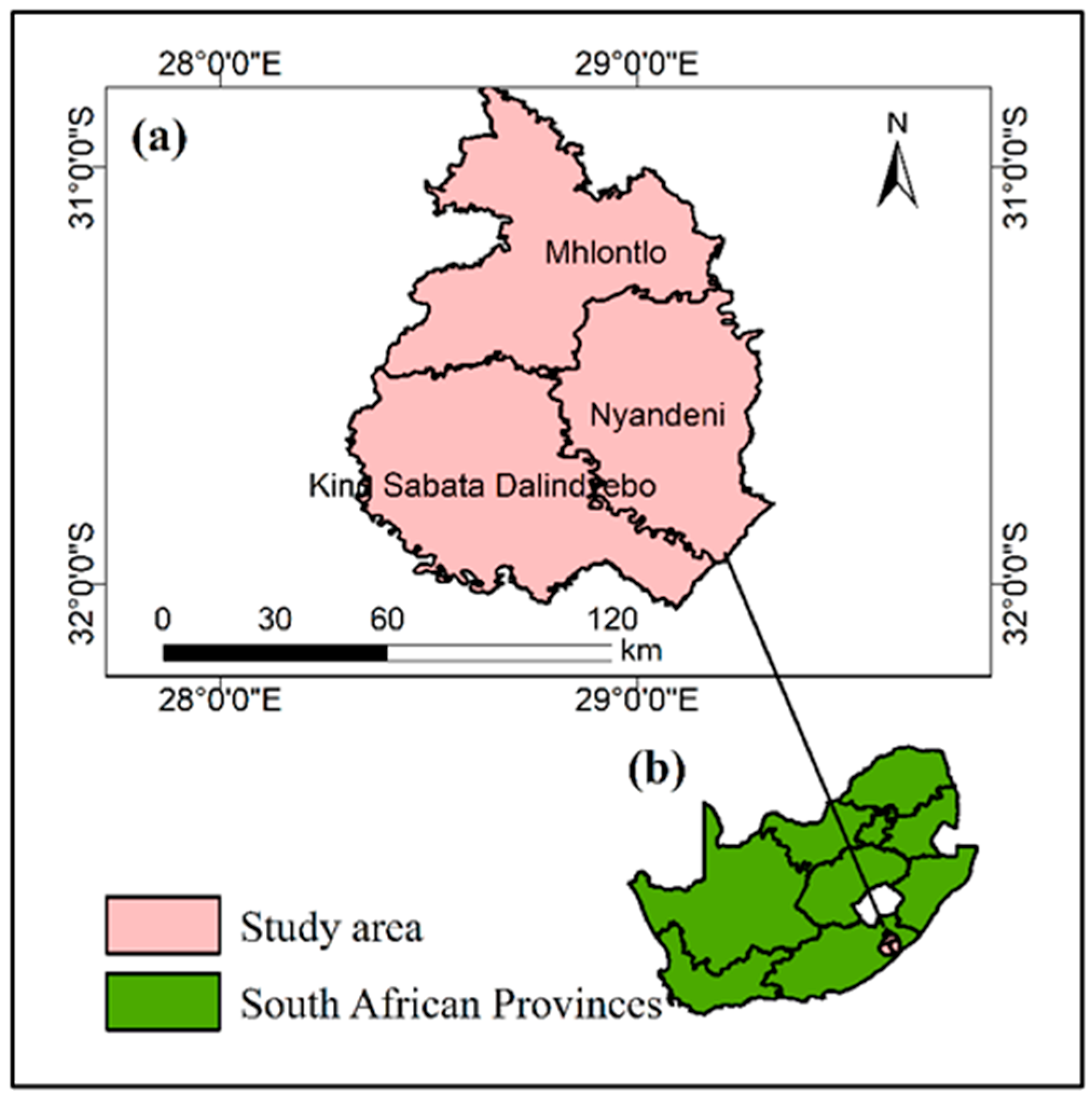
2.1. Study Area

The study focused on the ORTDM in the Eastern Cape Province of South Africa. ORTDM’s average annual rainfall ranges between 900 and 1300 mm. Summer or growing season temperatures range between 14 and 27 °C [40]. The physiography is characterized by densely vegetated undulating landscapes of 5 to 500 m elevations along the wild coast, gently-sloping grasslands in the interior and savannas and forests in the northern areas where elevation rises to 1500 m. The soils are sandy loams, sandy clay loams, and clays that are slightly acidic and yellow to black in color [41,42].

The study sites were located in ORTDM’s three local municipalities, which were King Sabata Dalindyebo (3027 km²), Nyandeni (2474 km²), and Mhlontlo (2826 km²) (Figure 1a). In these local municipalities, the study was limited around five weather stations, which are distributed within an area of approximately 70 × 50 km (Figure 2). More information about the study area is provided in Section 2.3.1 and Figure 2. The choice of this area was based on a list of maize producing farms that we obtained from the Department of Agriculture, Land Reform and Rural Development (DALRRD). Maize is the most important grain crop in South Africa; white maize is the major staple food and yellow maize is mostly used for feeding animals [43]. It is sown between October and early-January and harvested between June and August; however, some of the farmers plant late because of delayed delivery of inputs. Farmers and DALRRD officials indicated that the optimum planting window in the study area is 15 November to 31 December. Therefore, this study focused on the maize growing period, which coincides with the rainy season and spans between November and April. The cultivation records we obtained from the DALRRD show that target yield is five tons per hectare (t/ha). However, studies show that maize yields in ORTDM are low and often below five t/ha [18,44,45]. Currently, all of ORTDM’s maize farmers, including the majority of South Africa’s smallholder farmers, do not have any type of formal insurance [46,47,48].

2.2. Data

The rainfall data used in this study include (1) in-situ rainfall records from automatic weather stations (WSs), (2) TAMSAT and (3) CHIRPS data. Long-term averages of minimum and maximum temperatures, humidity, wind speed, and sunshine hours were obtained from the CLIMWAT database.

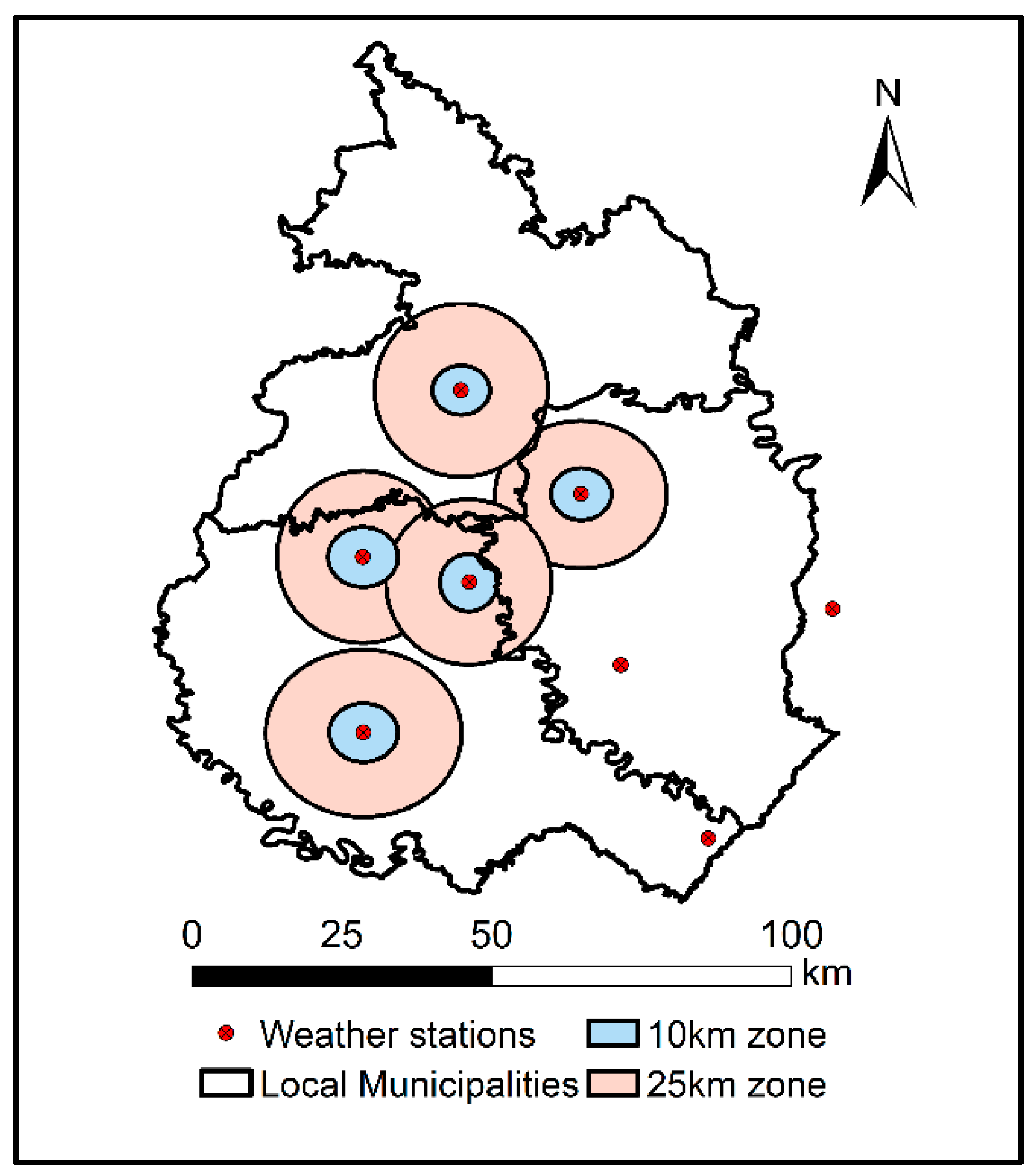
2.2.1. In-Situ Rainfall Data

In-situ rainfall records were obtained from the Agricultural Research Council’s agro-climate databank, which receives weather data from automatic WSs situated in Tsolo, Libode, Ross Mission, Qunu, and Mthatha (

Table 1. Locations of the weather stations.

Station Name	Latitude	Longitude
Tsolo	−31.2923	28.7627
Libode	−31.4481	28.9430
Ross Mission	−31.5427	28.6153
Qunu	−31.8060	28.6161
Mthatha	−31.5803	28.7754

). The study focused on the critical maize growing period, which is from November to April and covered the 18 seasons between 2002 and 2019. This period was selected because there were numerous missing data in the rainfall records of the manual WSs that were operating prior to 2002. The five WSs listed in Table 1 were selected because they are situated within the area that is suitable for growing maize. Although maize is also grown in the areas around the other three WSs shown in Figure 2, these areas have high rainfall and uneven terrain and are suitable for vegetables, fruits, and forestry [49].

2.2.2. TAMSAT

TAMSAT version 3.1 data covering 2002 to 2019 were downloaded from https://www.tamsat.org.uk/ (accessed on 20 September 2021). This dataset has a spatial resolution of 0.0375° and includes daily, pentadal, monthly, and seasonal rainfall products developed from thermal infrared satellite data and gauge-based rainfall data. The dataset is developed by the University of Reading. The approach used to estimate TAMSAT rainfall is based on the understanding that rainfall predominantly comes from convective cumulonimbus storm clouds [50]. Precipitation occurs when these clouds reach a certain temperature. TAMSAT infers this temperature from thermal infrared satellite imagery. The threshold temperature and the regression coefficients that estimate rainfall from the thermal imagery are determined by relating gauge observations to Cold Cloud Duration (CCD).

2.2.3. CHIRPS

CHIRPS data covering 2002 to 2019 were downloaded from https://climateserv.servirglobal.net/ (accessed on 19 September 2021). CHIRPS includes daily, pentadal, and monthly precipitation observations of 0.05° spatial resolution. This dataset is developed by the Climate Hazard Group and the United States Geological Survey’s Earth Resources Observation and Science Centre. CHIRPS is a product of multiple satellite datasets and gauge-based observations [51]. The data is produced in two phases in which; (1) World Meteorological Organisation’s Global Telecommunication System gauge data are blended with CCD rainfall estimates at every pentad and, (2) the best available monthly and pentadal station data are combined with CCD-based rainfall estimates.

2.2.4. Climate Data Used for Calculating CWR

We obtained long-term averages of minimum and maximum temperatures, humidity, wind speed, and sunshine hours from the CLIMWAT database. CLIMWAT is a climatic database that is used with the CROPWAT model to calculate CWR [52]. Of all the WSs in ORTDM, the CLIMWAT database only has climatic data of the Mthatha weather station (WS) (denoted as Umtata).

2.3. Data Preprocessing and Analysis

2.3.1. Preprocessing of In-Situ Rainfall Data

WS data were preprocessed and transformed to daily, 20-day cumulative, and monthly cumulative measurements covering November to April for each of the 18 seasons between 2002 and 2019. The 20-day and monthly time steps correspond to the lengths of the growth stages of maize as classified by the Food and Agriculture Organization (FAO) in the CROPWAT model [52]. These stages are the plant’s initial, development, mid-season, and late growth phase.

2.3.2. Preprocessing of SRFEs

A python script was used to extract time series rainfall values from CHIRPS images to comma separated values (CSV) files. TAMSAT data are provided in the form of source-compiled CSV files. Studies report that satellite-based rainfall estimates are better when spatially aggregated than in their native spatial resolutions [15,38]. Therefore, both CHIRPS and TAMSAT were spatially aggregated (Figure 2).

CHIRPS data were aggregated by averaging pixel values that lie within 5 and 12.5 km from the reference WS (Figure 2). TAMSAT data were aggregated to the same spatial scales using the sub-setting tool available in the TAMSAT website, which allows users to download spatially averaged values within a specified boundary. Both datasets were daily, 20-day cumulative, and monthly cumulative records covering November to April for each of the 18 seasons between 2002 and 2019

2.3.3. Evaluating TAMSAT and CHIRPS against In-Situ Rainfall Data

The SRFEs were evaluated against the WS data using Pearson’s correlation. Correlation analysis was purposefully selected because it has been used to validate satellite-based rainfall products [35,36,37] and to assess different satellite data in IBCI [15,38,39,40]. Of all the WSs in ORTDM, the Mthatha WS is the only one whose data are used for calibration by the developers of CHIRPS and TAMSAT (Table 1). Therefore, the SRFEs were evaluated against the other four WSs excluding the Mthatha WS. However, after evaluating and validating the SRFEs against these four WSs, we used the Mthatha WS for the next objective, which was calculate CWR and develop the IBCI payout structure.

2.3.4. Crop Water Requirements

Stagewise assessments of crop water requirements (CWR) were conducted using FAO’s CROPWAT 8.0 model [52]. CROPWAT is a computer model for calculating CWR and irrigation requirements based on soil, climate, and crop data [52,53]. CROPWAT can also be used to estimate crop performance under both rain-fed and irrigated conditions. This model has been used in South Africa by several studies to calculate evapotranspiration and CWR [54,55,56,57]. The model calculates growing season CWR or crop evapotranspiration ${\mathrm{ET}}_{\mathrm{c}}$ from reference evapotranspiration (ET₀) and crop coefficients (K_c) according to Equation (1).

$${\mathrm{ET}}_{\mathrm{c}}={ \mathrm{K}}_{\mathrm{c} }\times { \mathrm{ET}}_0$$

(1)

The calculation of ET₀ is based on the Penman-Monteith method and long-term average minimum and maximum temperatures, humidity, wind speed, and sunshine hours. Rainfall data were extracted from CHIRPS because CHIRPS outperformed TAMSAT. CWR were calculated for each of the earlier stated four growth stages of maize for a 120-day maturing variety. In South Africa, maize takes 120 or more days to mature [58,59,60]. Crop coefficients ${\mathrm{K}}_{\mathrm{c}}$ were based on FAO’s recommendations, which are available in the maize file provided in CROPWAT’s crop folder. Effective rainfall was calculated using the USDA soil conservation service method [61,62]. Lastly, rainfall deficits (RD) or irrigation water requirements, which indicate whether CWR are met or not, were calculated for each of the four growth stages. These calculations were carried out in order to (1) explore the possibility of using the CWR as the trigger threshold for IBCI, and (2) identify the most water-critical of the four growth stages of maize by comparing their CWR and RD.

2.3.5. IBCI Development and Payout Thresholds

Designing an IBCI involves determination of key thresholds, which are, (1) the trigger and exit thresholds, (2) the crop growth period over which the index is measured, (3) the tick, which is the payout frequency between the trigger and the exit, and (4) the insured amount. We adopted the approach used by Choudhury et al. [15] as well as Eze et al. [17] for the IBCI payout structure. However, instead of correlating crop yields and rainfall, we used CWR and long-term SRFEs to derive the trigger and exit thresholds. The payout structure is based on Equation (2);

$$\mathrm{Payout}=\{\begin{array}{c}{\mathrm{IA}}_{\mathrm{i}},\\ {\mathrm{IA}}_{\mathrm{i}}\\ 0,\end{array}\left(\frac{{\mathrm{T}}_{\mathrm{i}}-{\mathrm{A}}_{\mathrm{i}}}{{\mathrm{T}}_{\mathrm{i}}-{\mathrm{E}}_{\mathrm{i}}}\right), \begin{array}{c}{\mathrm{if} \mathrm{A}}_{\mathrm{i}} \le { \mathrm{E}}_{\mathrm{i}}\\ { \mathrm{if} \mathrm{E}}_{\mathrm{i}}<{\mathrm{A}}_{\mathrm{i}}\le {\mathrm{T}}_{\mathrm{i}}\\ {\mathrm{if} \mathrm{A}}_{\mathrm{i}}>{\mathrm{T}}_{\mathrm{i}}\end{array}$$

(2)

where,

• ${\mathrm{IA}}_{\mathrm{i}}$ is the insured amount for growth stage $\mathrm{i}$, which is a portion of the costs spent on inputs (seeds, fertilizers, pesticides, herbicides, land preparations, etc.) [17],
• ${\mathrm{A}}_{\mathrm{i}}$ is the actual index value of growth stage $\mathrm{i}$,
• ${\mathrm{T}}_{\mathrm{i}}$ is the trigger point at which payout starts, and
• ${\mathrm{E}}_{\mathrm{i}}$ is the exit threshold at which full payout is given.

when ${\mathrm{A}}_{\mathrm{i}}$ is equal to or below ${\mathrm{E}}_{\mathrm{i}}$, the farmer gets the entire insured amount for that growth stage. If ${\mathrm{A}}_{\mathrm{i}}$ is between ${\mathrm{T}}_{\mathrm{i}}$ and ${\mathrm{E}}_{\mathrm{i}}$, the system pays out a proportion of the amount according to ${\mathrm{IA}}_{\mathrm{i}}\left(\frac{{\mathrm{T}}_{\mathrm{i}}-{\mathrm{A}}_{\mathrm{i}}}{{\mathrm{T}}_{\mathrm{i}}-{\mathrm{E}}_{\mathrm{i}}}\right)$. When ${\mathrm{A}}_{\mathrm{i}}$ is above ${\mathrm{T}}_{\mathrm{i}}$, the system pays nothing. Following Chen et al. [63], the tick was derived using Equation (3). In this case, the tick is the amount insured for growth stage $\mathrm{i}$ divided by the difference between the trigger and the exit of growth stage $\mathrm{i}$.

$$\mathrm{Tick}=\frac{{\mathrm{IA}}_{\mathrm{i}}}{{\mathrm{T}}_{\mathrm{i}}-{\mathrm{E}}_{\mathrm{i}}}$$

(3)

The insured amount is equal to the sum of money spent on inputs and land preparation, which, according to the farmers and the DALRRD, is approximately R10,000 ($623.22 by 2 December 2021) per hectare. In an earlier study, Masiza et al. [64] demonstrated that information on hectarage and distributions of farms can be accurately derived by optimizing machine learning and remote sensing methods. A similar study used the same techniques and demonstrated that the approach is very accurate (p < 0.05, R = 0.84) in estimating crop hectarage [65].

To calculate the insurable amount for each growth stage, the stages were weighted according to RD. CROPWAT reports RD as irrigation water requirements. The weightings of the growth stages were based on RD and not on CWR because the calculation of RD takes into account both CWR and the actual rainfall received by the crop (i.e., RD = CWR − Effective Rainfall). The weight of growth stage $\mathrm{i}$, therefore, is given by the RD of growth stage $\mathrm{i}$ divided by the total RD of the four stages (Equation (4)).

$${\mathrm{Weight}}_{\mathrm{i}}=\frac{{\mathrm{RD}}_{\mathrm{i}}}{{{\displaystyle \sum }}_1^{\mathrm{n}}\mathrm{RD}}$$

(4)

The insurable amount for each stage is calculated according to Equation (5).

$${\mathrm{IA}}_{\mathrm{i}}={ \mathrm{Weight}}_{\mathrm{i}}\times \mathrm{R}10,000$$

(5)

3. Results

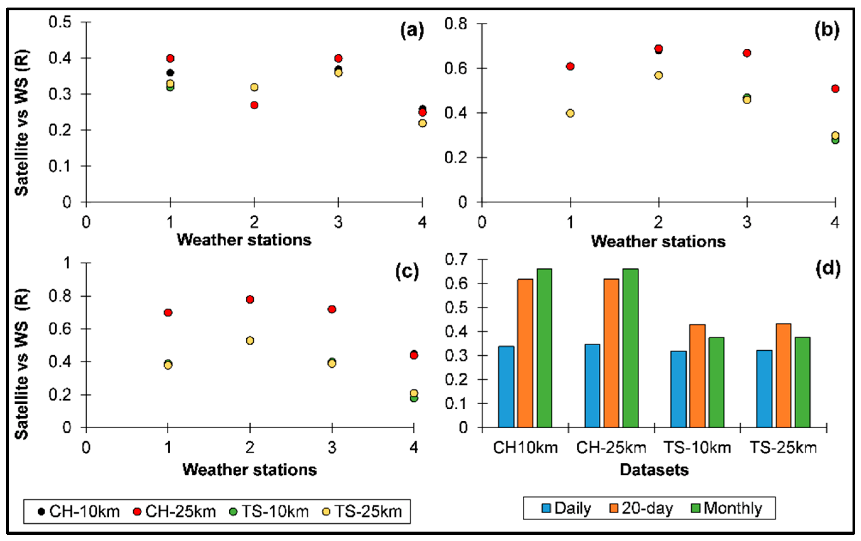
3.1. Correlations between Satellite and WS Data at Different Spatial and Temporal Scales

This subsection presents composite graphs that show correlations between satellite and WS data (Figure 3). Figure 3 shows how WS data and SRFEs (TS = TAMSAT, CH = CHIRPS) correlated at different spatial and temporal scales.

All correlations were statistically significant at the 95% confidence level with all p-values less than 0.05 except for the lowest correlations (R ≤ 0.21) between TAMSAT and WS data in Figure 3c. Correlations between daily CHIRPS and WS data were weak (R ≤ 0.40) and slightly weaker between daily TAMSAT and WS data (R ≤ 0.37) (Figure 3a). However, the results improved at the 20-day time step, with CHIRPS and WS data correlating by 0.51 to 0.68 at the 10 km scale and by 0.51 to 0.69 at the 25 km scale. Correlations between TAMSAT and WS data were lower with a maximum correlation of 0.57 (Figure 3b). At the monthly time step, CHIRPS agreed strongly with WS data by achieving maximum correlations of 0.78 at both spatial scales, while TAMSAT reached a moderate maximum of 0.53 (Figure 3c). Figure 3d summarizes Figure 3a–c by averaging the correlations for the four weather stations. Overall, CHIRPS outperformed TAMSAT at all the spatial and temporal scales and performed best at the monthly time step.

3.2. Crop Water Requirements Based on Different Planting Dates

Table 2. CWR when planting is on 21 November.

Planting Date	Stage	Days	CWR	ER *	RD	MR *	MMR *
21 November	Initial	20	25.20	50.40	0.00	67.07	37.79
	Development	30	102.30	83.70	18.60	90.22	63.92
	Mid-season	40	201.00	115.10	85.90	141.98	109.63
	Late season	30	73.50	86.40	0.00	94.58	26.84
	Total	120	402.00	335.60	104.50	393.82	238.18
1 December	Initial	20	25.20	52.80	0.00	62.23	47.76
	Development	30	103.20	86.50	16.70	92.03	66.59
	Mid-season	40	184.20	113.10	71.10	146.74	108.17
	Late season	30	78.20	81.30	0.00	96.45	75.74
	Total	120	390.80	333.70	87.80	397.45	298.26
11 December	Initial	20	26.80	54.80	0.00	54.51	26.60
	Development	30	105.30	87.90	17.40	100.62	84.21
	Mid-season	40	170.70	112.90	57.80	137.10	109.03
	Late season	30	74.20	72.10	2.10	87.88	25.93
	Total	120	377.00	327.70	77.30	380.11	245.77
21 December	Initial	20	27.20	56.70	0.00	65.22	26.53
	Development	30	102.40	87.30	15.10	96.27	52.40
	Mid-season	40	163.00	114.20	48.80	140.87	73.55
	Late season	30	70.30	58.20	12.10	67.52	24.94
	Total	120	362.90	316.40	76.00	369.88	177.42

* ER = Effective Rainfall, MR = Mean Rainfall, MMR = Mean Minimum Rainfall.

shows the results of CWR assessment for maize planted on different dates. The metric unit for rainfall and CWR is millimeters (mm). CWR were calculated using long-term climate data.

For all the four planting dates, the initial growth stage has the lowest CWR and the mid-season stage has the highest (Table 2). The late-season and development stages have the second-lowest and second-highest CWR, respectively. For all the four planting dates, the initial stage gets enough effective rainfall and no RD. When planting is on 21 November or 1 December, the late-season period also has no RD, whereas planting on 11 December or 21 December results in late-season RD. The mid-season period has the highest RD followed by the development stage. The initial stage has the lowest rainfall across all planting dates, while the mid-season period has the highest. Planting on 21 November or 1 December results in the late-season period receiving the second-highest rainfall, whereas planting on 11 December or 21 December results in the development stage receiving the second-highest rainfall.

3.3. Insurance Threshold Values

The index thresholds presented in

Table 3. Index threshold values for maize planted on 21 December.

Growth Stages	Trigger (mm)	Exit (mm)	Tick (R/mm)	Weight	Amount (R)
Development	96.27	52.40	45.59	0.20	2000
Mid-season	140.87	73.55	95.07	0.64	6400
Late-season	67.52	24.94	37.58	0.16	1600

are based on the results presented in Section 3.2 and on Equations (2)–(5). The thresholds are based on the optimum planting date, which was 21 December. The optimum planting date may change from year to year; the optimum planting date in this case is based on long-term data. The selection of this date was based on the following considerations:

• First, we observed that total seasonal and mid-season CWR decrease with delayed planting. In other words, planting on 21 December results in less CWR than planting on 11 December, 1 December, and 21 November;
• Second, total seasonal and mid-season RD also decrease with delayed planting. In other words, planting on 21 December results in less RD than planting earlier;
• Third, the mid-season stage is given more weight because it has the highest CWR and RD, and it is the most water-sensitive growth stage;
• Fourth, a planting date that evenly and proportionately distributes CWR and RD across multiple stages is less risky;
• Fifth, the farmers’ experiences and historical planting dates were considered.

Based on these factors, 21 December was selected as the optimum planting date because it meets the first two of the considerations listed above. 21 December is also the date on which the most important stage (i.e., the mid-season) has the lowest RD. Lastly, 21 December meets the fourth consideration because it evenly and proportionately distributes CWR and RD across all the growth stages. This date was then used to develop the proposed payout structure. However, instead of using CWR, the study used long-term mean-total and mean-minimum rainfall as trigger and exit points (Table 3). The choice of these thresholds is explained in the discussion section. The most crucial growth stages for a planting date of 21 December are the development, mid-season, and late-season stages. Since the initial growth stage has enough effective rainfall and zero RD (Table 2), this stage has zero weight. The development stage has a weight of 20%, the mid-season stage has a weight of 64%, and the late-season stage has a weight of 16%. For each millimeter of rainfall below the trigger point, amounts of R45.59, R95.07, and R37.58 are paid out for the development, mid-season, and late-season stages, respectively (Table 3).

4. Discussions and Conclusions

4.1. Satellite Data for IBCI Design

The first objective of this study was to assess the performances of CHIRPS and TAMSAT datasets in estimating rainfall at different spatial and temporal scales in ORTDM. These datasets performed better at 20-day and monthly time-steps, with CHIRPS consistently performing better than TAMSAT. The superiority of CHIRPS over TAMSAT is also reported in other studies [66,67,68]. The different spatial scales at which the analyses were carried out did not influence the performances of these datasets. This means that, CHIRPS data, aggregated to any spatial scale between 10 × 10 km and 25 × 25 km, can fairly represent the local rainfall conditions in ORTDM. This finding is supported by Duplessis and Kibii [69], who found that monthly CHIRPS data estimated rainfall very well in 46 locations across South Africa, with an average R² of 0.60. In the Eastern Cape, Mhalalela et al. [70] also found significant correlations ranging between 0.61 and 0.90 between CHIRPS and WS data. However, these findings must be interpreted with caution as SRFEs’ ability to estimate rainfall depends on the climate and physiography of the area. It is reported that SRFEs tend to misestimate rainfall in coastal and mountainous areas [38,39,67,68]. Therefore, since insurance requires reliable and good quality data to minimize basis risk, SRFEs must be validated and compared with in-situ rainfall and other rainfall-related datasets [16,71,72]. Nevertheless, since CHIRPS performed well in ORTDM, this dataset can be used in conjunction with agro-ecological information to demarcate unit areas of insurance. In addition, since CHIRPS performed well at 20-day and monthly time-steps, this dataset can also be used to develop indices for the different growth stages of maize, which range in length between 20 and 40 days. The study, therefore, proceeded to use CHIRPS in the assessment of CWR and the design of the IBCI payout structure.

4.2. Maize Water Requirements and IBCI Design

It is evident from the results that, regardless of the planting date, the average seasonal CWR exceed seasonal rainfall, resulting in RD. These RD are minimal when planting is on 21 December. Although RD pose a challenge to rain-fed maize, the initial stage, which corresponds to germination, emergence and early vegetative stages, receives sufficient rainfall. This scenario implies that the initial stage is less prone to water deficits and has zero weight. It also validates the perception that 21 November to 21 December is a suitable planting window for ORTDM. Therefore, the index is not measured over the initial stage. Although IBCI programs such as the R4 rural resilience initiative, ACRE Africa, and others cover germination failure [7,73], RD-induced germination failure is unlikely to occur in ORTDM if maize is planted between 21 November and 21 December. However, since germination failure is compensated for by replanting, farmers can still be indemnified with the amount of money needed for replanting when RD-induced germination failure occurs.

The development and mid-season stages’ RD decrease with delayed planting, whereas the late-season stage’s RD increase with delayed planting. Remember, rainfall deficit is the difference between CWR and rainfall (Table 2). If RD are likely to occur every year as the results show, insurance cannot compensate for these RD. This means that CWR cannot be used as the trigger threshold as this study initially intended. However, studies report that the weather conditions of ORTDM can produce good yields when inputs are managed properly [18,42,74]. This is supported by Osgood et al. [75], who observed that crops that are adapted to the prevalent local climate conditions have low vulnerability during dry spells. They [75] also point out that the parameters of CWR models are not a definite predictor of crop behavior. It is for these reasons that long-term mean and mean-minimum rainfall were used as trigger and exit thresholds, respectively. Therefore, the proposed system uses long-term mean and mean-minimum rainfall as thresholds; the rainfall data is derived from CHIRPS; the system measures the index over the development, mid-season, and late-season stages and it operates on a linear payout structure as shown in Figure 4.

The model gives more weight to the mid-season stage, which corresponds to the late vegetative, tasseling, silking, pollination, and blister stages. It is over these growth stages that water and nutrient demands are high [58,76,77]. The late-season stage has the lowest weight because it has lower CWR and RD than the development and mid-season stages. Measuring the index over the critical crop growth stages rather than measuring it once at the end of the season potentially reduces temporal basis risk. The key contribution of this study is the derivation of index thresholds from CWR and site-specific rainfall conditions. The widely used approach, which calibrates IBCI by correlating yields and rainfall exposes contracts to basis risk because, by simply correlating yield and rainfall data, it overlooks the influence of non-weather factors on smallholder crop yields and losses [26]. However, the approach used in this study is informed by the fact that, in most cases, rainfall-related yield reduction results from rainfall deficit, which is the failure of rainfall to meet CWR. Although the approach proposed in this study is premised on the prevailing conditions in ORTDM and South Africa, it can be applied in other areas with different growing conditions. More research can improve this approach by investigating the relationship between RD and yield losses under controlled and well-managed non-weather yield-determining factors.

References

1. Langyintuo, A. Smallholder farmers’ access to inputs and finance in Africa. In The Role of Smallholder Farms in Food and Nutrition Security; Paloma, S., Riesgo, L., Louhichi, K., Eds.; Springer International Publishing: Cham, Switzerland, 2020; pp. 133–152. [Google Scholar] [CrossRef]
2. Akinnagbe, O.M.; Irohibe, I.J. Agricultural adaptation strategies to climate change impacts in Africa: A review. Bangladesh J. Agric. 2014, 39, 407–418. [Google Scholar] [CrossRef]
3. Sultan, B.; Defrance, D.; Iizumi, T. Evidence of crop production losses in West Africa due to historical global warming in two crop models. Sci. Rep. 2019, 9, 1–15. [Google Scholar] [CrossRef] [Green Version]
4. Buhaug, H.; Benaminsen, T.A.; Sjaastad, E.; Magnus Theisen, O. Climate variability, food production shocks, and violent conflict in Sub-Saharan Africa. Environ. Res. Lett. 2015, 10, 125015. [Google Scholar] [CrossRef]
5. Gebremeskel, G.; Tang, Q.; Sun, S.; Huang, Z.; Zhang, X.; Liu, X. Droughts in East Africa: Causes, impacts and resilience. Earth-Sci. Rev. 2019, 193, 146–161. [Google Scholar] [CrossRef]
6. ACRE. 3-D Client Value Assessment for ACRE Rwanda Maize & Livestock Insurance Products; ACRE: Nairobi, Kenya, 2020; Available online: https://acreafrica.com/ (accessed on 26 May 2021).
7. WFP. R4 Rural Resilience Initiative: Annual Report; WFP: Rome, Italy, 2020; Available online: https://www.wfp.org/publications/r4-rural-resilience-initiative-2020-annual-report (accessed on 4 February 2021).
8. Sharoff, J.; Diro, R.L.; McCarney, G.; Norton, M. R4 Rural Resilience Initiative in Ethiopia. Clim. Serv. Partnersh. 2015, 1–7. Available online: https://www.climate-services.org/wp-content/uploads/2015/09/R4_Ethiopia_Case_Study.pdf (accessed on 18 January 2021).
9. ARC. Africa RiskView: End of Season Report|Malawi (2020/21 Season); ARC: Johannesburg, South Africa, 2020. [Google Scholar]
10. Hernandez, E.; Goslinga, R.; Wang, V. Using Satellite Data to Scale Smallholder Agricultural Insurance; CGAP: Washington, DC, USA, 2018; Available online: https://www.cgap.org/sites/default/files/Brief-Using-Satellite-Data-Smallholder-Agricultural-Insurance-Aug-2018.pdf (accessed on 18 June 2019).
11. Barnett, B.J.; Mahul, O. Weather index insurance for agriculture and rural areas in lower-income countries. Am. J. Agric. Econ. 2007, 89, 1241–1247. [Google Scholar] [CrossRef]
12. Ntukamazina, N.; Onwonga, R.N.; Sommer, R.; Rubyogo, J.C.; Mukankusi, C.M.; Mburu, J.; Kariuki, R. Index-based agricultural insurance products: Challenges, opportunities and prospects for uptake in sub-Sahara Africa. J. Agric. Rural Dev. Trop. Subtrop. 2017, 118, 171–185. Available online: https://www.jarts.info/index.php/jarts/article/view/2017042052372 (accessed on 13 May 2019).
13. Tadesse, M.A.; Shiferaw, B.A.; Erenstein, O. Weather index insurance for managing drought risk in smallholder agriculture: Lessons and policy implications for sub-Saharan Africa. Agric. Food Econ. 2015, 3, 1–21. [Google Scholar] [CrossRef] [Green Version]
14. Clement, K.Y.; Wouter Botzen, W.J.; Brouwer, R.; Aerts, J.C.J.H. A global review of the impact of basis risk on the functioning of and demand for index insurance. Int. J. Disaster Risk Reduct. 2018, 28, 845–853. [Google Scholar] [CrossRef]
15. Choudhury, A.; Jones, J.; Okine, A.; Choudhury, R.L. Drought-triggered index insurance using cluster analysis of rainfall affected by climate change. J. Insur. Issues 2016, 39, 169–186. Available online: https://www.jstor.org/stable/43921956 (accessed on 16 February 2020).
16. Enenkel, M.; Osgood, D.; Anderson, M.; Powell, B.; McCarty, J.; Neigh, C.; Carroll, M.; Wooten, M.; Husak, G.; Hain, C.; et al. Exploiting the convergence of evidence in satellite data for advanced weather index insurance design. Weather Clim. Soc. 2019, 11, 65–93. [Google Scholar] [CrossRef]
17. Eze, E.; Girma, A.; Zenebe, A.A.; Zenebe, G. Feasible crop insurance indexes for drought risk management in Northern Ethiopia. Int. J. Disaster Risk Reduct. 2020, 47, 101544. [Google Scholar] [CrossRef]
18. Masiza, W.; Chirima, J.; Hamandawana, H.; Kalumba, A.M.; Magagula, H.B. Linking agricultural index insurance with factors that influence maize yield in rain-fed smallholder farming systems. Sustainability 2021, 13, 5176. [Google Scholar] [CrossRef]
19. Gornott, C.; Hattermann, F.; Wechsung, F. Yield gap analysis for Tanzania—The impacts of climate, management, and socio-economic impacts on maize yields. Procedia Environ. Sci. 2015, 29, 231. [Google Scholar] [CrossRef] [Green Version]
20. Kihara, J.; Tamene, L.D.; Massawe, P.; Bekunda, M. Agronomic survey to assess crop yield, controlling factors and management implications: A case-study of Babati in northern Tanzania. Nutr. Cycl. Agroecosyst. 2015, 102, 5–16. [Google Scholar] [CrossRef] [Green Version]
21. Beza, E.; Silva, J.V.; Kooistra, L.; Reidsma, P. Review of yield gap explaining factors and opportunities for alternative data collection approaches. Eur. J. Agron. 2017, 82, 206–222. [Google Scholar] [CrossRef]
22. MacCarthy, D.S.; Adiku, S.G.; Freduah, B.S.; Kamara, A.Y.; Narh, S.; Abdulai, A.L. Evaluating maize yield variability and gaps in two agroecologies in northern Ghana using a crop simulation model. S. Afr. J. Plant Soil 2018, 35, 137–147. [Google Scholar] [CrossRef] [Green Version]
23. Assefa, B.T.; Chamberlin, J.; Reidsma, P.; Silva, J.V.; van Ittersum, M.K. Unravelling the variability and causes of smallholder maize yield gaps in Ethiopia. Food Secur. 2020, 12, 489–490. [Google Scholar] [CrossRef] [Green Version]
24. Dutta, S.; Chakraborty, S.; Goswami, R.; Banerjee, H.; Majumdar, K.; Li, B.; Jat, M.L. Maize yield in smallholder agriculture system—An approach integrating socio-economic and crop management factors. PLoS ONE 2020, 15, e0229100. [Google Scholar] [CrossRef] [PubMed]
25. Banerjee, H.; Goswami, R.; Chakraborty, S.; Dutta, S.; Majumdar, K.; Satyanarayana, T.; Jat, M.L.; Zingore, S. Understanding biophysical and socio-economic determinants of maize (Zea mays L.) yield variability in eastern India. NJAS-Wagening. J. Life Sci. 2014, 70, 79–93. [Google Scholar] [CrossRef] [Green Version]
26. Masiza, W.; Chirima, G.J.; Hamandawana, H.; Kalumba, A.M.; Magagula, H.B. Do satellite data correlate with in-situ rainfall and smallholder crop yields? Implications for crop insurance. Sustainability 2022, 14, 1670. [Google Scholar] [CrossRef]
27. Carletto, C.; Jolliffe, D.; Banerjee, R. The Emperor Has No Data! Agricultural Statistics in Sub-Saharan Africa. World Bank Working Paper. 2013. Available online: http://mortenjerven.com/wp-content/uploads/2013/04/Panel-3-Carletto.pdf (accessed on 16 March 2018).
28. Djurfeldt, G.; Hall, O.; Jirström, M.; Archila Bustos, M.; Holmquist, B.; Nasrin, S. Using panel survey and remote sensing data to explain yield gaps for maize in sub-Saharan Africa. J. Land Use Sci. 2018, 13, 344–357. [Google Scholar] [CrossRef] [Green Version]
29. Osgood, D.; Powell, B.; Diro, R.; Farah, C.; Enenkel, M.; Brown, M.E.; Husak, G.; Blakeley, L.; Hoffman, L.; McCarty, J.L. Farmer perception, recollection, and remote sensing in weather index insurance: An Ethiopia case study. Remote Sens. 2018, 10, 1887. [Google Scholar] [CrossRef] [Green Version]
30. Pereira, L.S.; Alves, I. Crop. Water Requirements; Elsevier Inc.: Amsterdam, The Netherlands, 2013. [Google Scholar] [CrossRef]
31. Wani, S.P.; Sreedevi, T.K.; Rockström, J.; Ramakrishna, Y.S. Rainfed agriculture—Past trends and future prospects. In Rainfed Agriculture: Unlocking the Potential; Wani, S.P., Sreedevi, T.K., Rockström, J., Ramakrishna, Y.S., Eds.; CABI: Wallingford, UK, 2009; pp. 1–35. [Google Scholar] [CrossRef] [Green Version]
32. Worldbank. Weather Index Insurance for Agriculture: Guidance for Development Practitioners; Worldbank: Washington, DC, USA, 2011; Available online: https://documents1.worldbank.org/curated/en/590721468155130451/pdf/662740NWP0Box30or0Ag020110final0web.pdf (accessed on 11 February 2022).
33. Belissa, T.; Bulte, E.; Cecchi, F.; Gangopadhyay, S.; Lensink, R. Liquidity constraints, informal institutions, and the adoption of weather insurance: A randomized controlled trial in Ethiopia. J. Dev. Econ. 2019, 140, 269–278. [Google Scholar] [CrossRef]
34. Alcaide, K.D.R.; Buncag, M.J.J.; Mendoza, R.E.S.; Santos, L.B.U. Developing a Rainfall-Based Index for Corn Crop Insurance in Isabela, Philippines. Int. J. Sci. Manag. Stud. 2019, 2, 77–84. [Google Scholar] [CrossRef]
35. Butts-Wilmsmeyer, C.J.; Seebauer, J.R.; Singleton, L.; Below, F.E. Weather during key growth stages explains grain quality and yield of maize. Agronomy 2019, 9, 16. [Google Scholar] [CrossRef] [Green Version]
36. Çakir, R. Effect of water stress at different development stages on vegetative and reproductive growth of corn. F. Crop. Res. 2004, 89, 1–16. [Google Scholar] [CrossRef]
37. Song, L.; Jin, J.; He, J. Effects of severe water stress on maize growth processes in the field. Sustainability 2019, 11, 5086. [Google Scholar] [CrossRef] [Green Version]
38. Le Coz, C.; Van De Giesen, N. Comparison of rainfall products over sub-saharan africa. J. Hydrometeorol. 2020, 21, 553–596. [Google Scholar] [CrossRef]
39. Gebremicael, T.; Mohamed, Y.; van der Zaag, P.; Berhe, A.G.; Haile, G.G.; Hagos, E.Y.; Hagos, M.K. Comparison and validation of eight satellite rainfall products over the rugged topography of Tekeze-Atbara Basin at different spatial and temporal scales. Hydrol. Earth Syst. Sci. Discuss. 2017, 1–31, preprint. [Google Scholar] [CrossRef] [Green Version]
40. Jordaan, A.; Makate, D.; Mashego, T.; Mdungela, N.; Phatudi-Mphahlele, B.; Mashimbye, C.; Mlambo, D. Vulnerability Adaptation to and Coping with Drought: The Case of Commercial and Subsistence Rain Fed Farming in the Eastern Cape; Water Research Commission: Pretoria, South Africa, 2017; Available online: www.wrc.org.za (accessed on 6 June 2018).
41. Eta, N.E.; Grace, G. Investigation of some physicochemical charactyeristics/prperties of geophagic soil in the Oliver Tambo District Munucipality in the Eastern cape. Acad. J. Sci. 2013, 2, 465–471. [Google Scholar]
42. Sibanda, M.; Mushunje, A.; Mutengwa, C.S. An evaluation on the profitability of growing improved maize open pollinated varieties in the Eastern Cape Province, South Africa. J. Dev. Agric. Econ. 2016, 8, 1–13. [Google Scholar] [CrossRef] [Green Version]
43. DALRRD. Trends in the Agricultural Sector; DALRRD: Pretoria, South Africa, 2018. Available online: https://www.dalrrd.gov.za (accessed on 15 November 2018).
44. Chimonyo, V.G.P.; Mutengwa, C.; Chiduza, C.; Tandzi, L. Participatory variety selection of maize genotypes in the Eastern cape province of South Africa. S. Afr. J. Agric. Ext. 2019, 47, 103–117. [Google Scholar] [CrossRef] [Green Version]
45. Chimonyo, V.G.P.; Mutengwa, C.; Chiduza, C.; Tandzi, L. Characteristics of maize growing farmers, varietal use, and constraints to increase productivity in selected villages in the Eastern Cape province of South Africa. S. Afr. J. Agric. Ext. 2020, 48, 71–77. [Google Scholar] [CrossRef]
46. NAMC. Agripreneur: Agriculture Insurance; NAMC: Pretoria, South Africa, 2020; Available online: https://www.namc.co.za/wp-content/uploads/2020/04/Agrepreneur-Issue-20-March-2020.pdf (accessed on 13 February 2022).
47. Partridge, A.G.; Wagner, N.J. Risky business: Agricultural insurance in the face of climate change: Elsenburg journal. Agriprobe 2016, 13, 49–53. [Google Scholar] [CrossRef]
48. Elum, Z.A.; Modise, D.M.; Marr, A. Farmer’s perception of climate change and responsive strategies in three selected provinces of South Africa. Clim. Risk Manag. 2017, 16, 246–257. [Google Scholar] [CrossRef]
49. Nyandeni Local Municipality. Nyandeni Local Municipality: Local Economic Development Strategy Review; Nyandeni Local Municipality: Libode, South Africa, 2018. Available online: https://www.nyandenilm.gov.za/wp-content/uploads/2019/08/Final-Nyandeni-LM-LED-Strategy-Review-pdf (accessed on 18 November 2020).
50. Maidment, R.; Black, E.; Greatrex, H.; Young, M. TAMSAT. In Satellite Precipitation Measurement; Levizzani, V., Kidd, C., Kirschbaum, D., Eds.; Springer: Cham, Switzerland, 2020. [Google Scholar] [CrossRef]
51. Funk, C.; Peterson, P.; Landsfeld, M.; Pedreros, D.; Verdin, J.; Shukla, S.; Husak, S.; Rowland, J.; Harrison, L.; Hoell, A.; et al. The climate hazards infrared precipitation with stations—A new environmental record for monitoring extremes. Sci. Data. 2015, 2, 1–21. [Google Scholar] [CrossRef] [PubMed] [Green Version]
52. Smith, M.; Kivumbi, D.; Heng, L. Use of the FAO CROPWAT Model in Deficit Irrigation Studies; FAO: Rome, Italy, 2002; pp. 17–27. Available online: https://agris.fao.org/agris-search/search.do?recordID=XF2002407869 (accessed on 6 February 2019).
53. Muhammad, N. Simulation of maize crop under irrigated and rainfed conditions with CROPWAT model. J. Agric. Biol. Sci. 2009, 4, 68–73. Available online: http://www.arpnjournals.com/jabs/research_papers/rp_2009/jabs_0309_123.pdf (accessed on 18 November 2021).
54. Nyambo, P.; Wakindiki, I.I.C. Water footprint of growing vegetables in selected smallholder irrigation schemes in South Africa. Water SA 2015, 41, 571–578. [Google Scholar] [CrossRef] [Green Version]
55. Worldbank. Actual Crop. Water Use in Project Countries—A Synthesis at the Regional Level; Worldbank: Washington, DC, USA, 2007; Volume 4288, Available online: https://elibrary.worldbank.org/doi/abs/10.1596/1813-9450-4288 (accessed on 10 February 2022).
56. Singo, L.R.; Kundu, P.; Mathivha, F. Spatial variation of reference evapotranspiration and its influence on the hydrology of Luvuvhu River Catchment. Res. J. Agric. Environ. Manag. 2016, 5, 187–196. Available online: https://univendspace.univen.ac.za/handle/11602/1265 (accessed on 10 February 2022).
57. Dabrowski, J.M.; Murray, K.; Ashton, P.J.; Leaner, J.J. Agricultural impacts on water quality and implications for virtual water trading decisions. Ecol. Econ. 2009, 68, 1074–1082. [Google Scholar] [CrossRef]
58. du Plessis, J. Maize Production; DALRRD: Pretoria, South Africa, 2003. [Google Scholar] [CrossRef]
59. Frost, C.; Thiebaut, N.; Newby, T. Evaluating Terra MODIS satellite sensor data products for maize yield estimation in South Africa. S. Afr. J. Geomat. 2013, 2, 106–119. [Google Scholar]
60. Masupha, T.E.; Moeletsi, M.E. The use of Water Requirement Satisfaction Index for assessing agricultural drought on rain-fed maize, in the Luvuvhu River catchment, South Africa. Agric. Water Manag. 2020, 237, 106142. [Google Scholar] [CrossRef]
61. Ali, M.; Mubarak, S. Effective rainfall calculation methods for field crops: An overview, analysis and new formulation. Asian Res. J. Agric. 2017, 7, 1–12. [Google Scholar] [CrossRef]
62. Bokke, A.S.; Shoro, K.E. Impact of effective rainfall on net irrigation water requirement: The case of Ethiopia. Water Sci. 2020, 34, 155–163. [Google Scholar] [CrossRef]
63. Chen, W.; Hohl, R.; Tiong, L.K. Rainfall index insurance for corn farmers in Shandong based on high-resolution weather and yield data. Agric. Financ. Rev. 2017, 77, 337–354. [Google Scholar] [CrossRef]
64. Masiza, W.; Chirima, J.; Hamandawana, H.; Pillay, R. Enhanced mapping of a smallholder crop farming landscape through image fusion and model stacking. Int. J. Remote Sens. 2020, 41, 8739–8756. [Google Scholar] [CrossRef]
65. Mashaba-Munghemezulu, Z.; Chirima, G.J.; Munghemezulu, C. Delineating smallholder maize farms from sentinel-1 coupled with sentinel-2 data using machine learning. Sustainability 2021, 13, 4728. [Google Scholar] [CrossRef]
66. Dinku, T.; Funk, C.; Peterson, P.; Maidment, R.; Tadesse, T.; Gadain, H.; Ceccato, P. Validation of the CHIRPS satellite rainfall estimates over eastern Africa. Q. J. R. Meteorol. Soc. 2018, 144, 292–312. [Google Scholar] [CrossRef] [Green Version]
67. Kimani, M.W.; Hoedjes, J.C.B.; Su, Z. An assessment of satellite-derived rainfall products relative to ground observations over East Africa. Remote Sens. 2017, 9, 430. [Google Scholar] [CrossRef] [Green Version]
68. Tarnavsky, E.; Chavez, E.; Boogaard, H. Agro-meteorological risks to maize production in Tanzania: Sensitivity of an adapted Water Requirements Satisfaction Index (WRSI) model to rainfall. Int. J. Appl. Earth Obs. Geoinf. 2018, 73, 77–87. [Google Scholar] [CrossRef]
69. DuPlessis, K.; Kibii, J. Applicability of CHIRPS-based satellite rainfall estimates for South Africa. J. S. Afr. Inst. Civ. Eng. 2021, 63, 43–54. [Google Scholar] [CrossRef]
70. Mahlalela, P.T.; Blamey, R.C.; Hart, N.C.G.; Reason, C.J.C. Drought in the Eastern Cape region of South Africa and trends in rainfall characteristics. Clim. Dyn. 2020, 55, 2743–2759. [Google Scholar] [CrossRef] [PubMed]
71. Enenkel, M.; Osgood, D.; Powell, B. The added value of satellite soil moisture for agricultural index insurance. In Remote Sensing of Hydrometeorological Hazards; Petropoulos, G.P., Islam, T., Eds.; CRS Press: Boca Raton, FL, USA, 2017; pp. 69–83. [Google Scholar] [CrossRef]
72. Enenkel, M.; Farah, C.; Hain, C.; White, A.; Anderson, M.; You, L.; Wagner, W.; Osgood, D. What rainfall does not tell us—enhancing financial instruments with satellite-derived soil moisture and evaporative stress. Remote Sens. 2018, 10, 1819. [Google Scholar] [CrossRef] [Green Version]
73. Arce, C. Comparative Assessment of Weather Index Insurance Strategies in Sub-Saharan Africa; Vuna Africa: Pretoria, South Africa, 2016; Available online: http://www.vuna-africa.com (accessed on 19 August 2019).
74. Sibanda, M.; Mushunje, A.; Mutengwa, C. Factors influencing the demand for improved maize open pollinated varieties (OPVs) by smallholder farmers in the Eastern Cape Province, South Africa. J. Cereals Oilseeds 2016, 7, 14–26. [Google Scholar] [CrossRef] [Green Version]
75. Osgood, D.; Mclaurin, M.; Carriquiry, M.; Mishra, A.; Fiondella, F.; Hansen, J.W.; Peterson, N.; Ward, M.N. Designing Weather Insurance Contracts for Farmers in Malawi, Tanzania, and Kenya; International Research Institute for Climate and Society (IRI), Columbia University: New York, NY, USA, 2007; Available online: https://iri.columbia.edu/~deo/IRI-CRMG-Africa-Insurance-Report-6-2007/IRI-CRMG-Kenya-Tanzania-Malawi-Insurance-Report-6-2007.pdf (accessed on 15 March 2018).
76. Masupha, T.E.; Moeletsi, M.E. Use of standardized precipitation evapotranspiration index to investigate drought relative to maize, in the Luvuvhu River catchment area, South Africa. Phys. Chem. Earth. 2017, 102, 1–9. [Google Scholar] [CrossRef]
77. Udom, B.E.; Kamalu, O.J. Crop water requirements during growth period of maize (Zea mays L.) in a moderate permeability soil on coastal Plain sands. Int. J. Plant. Res. 2019, 2019, 1–7. [Google Scholar] [CrossRef]
Figure 1. Study area (a) within South Africa (b).
Remotesensing 14 01512 g001
Figure 2. WSs and the spatial scales at which analyses were performed. Source: adapted from [26].
Remotesensing 14 01512 g002
Figure 3. Correlations of WS and satellite data at (a) daily, (b) 20-day, and (c) monthly intervals. (d) Mean correlations between WS and satellite data.
Remotesensing 14 01512 g003
Figure 4. Development stage (trigger = 96.27 mm, exit = 52.40 mm), mid-season (trigger = 140.87 mm, exit = 73.55 mm), late-season (trigger = 67.52 mm, exit = 24.94 mm).
Remotesensing 14 01512 g004