
Two-Stream Swin Transformer with Differentiable Sobel Operator for Remote Sensing Image Classification


Abstract
:1. Introduction
- (1)
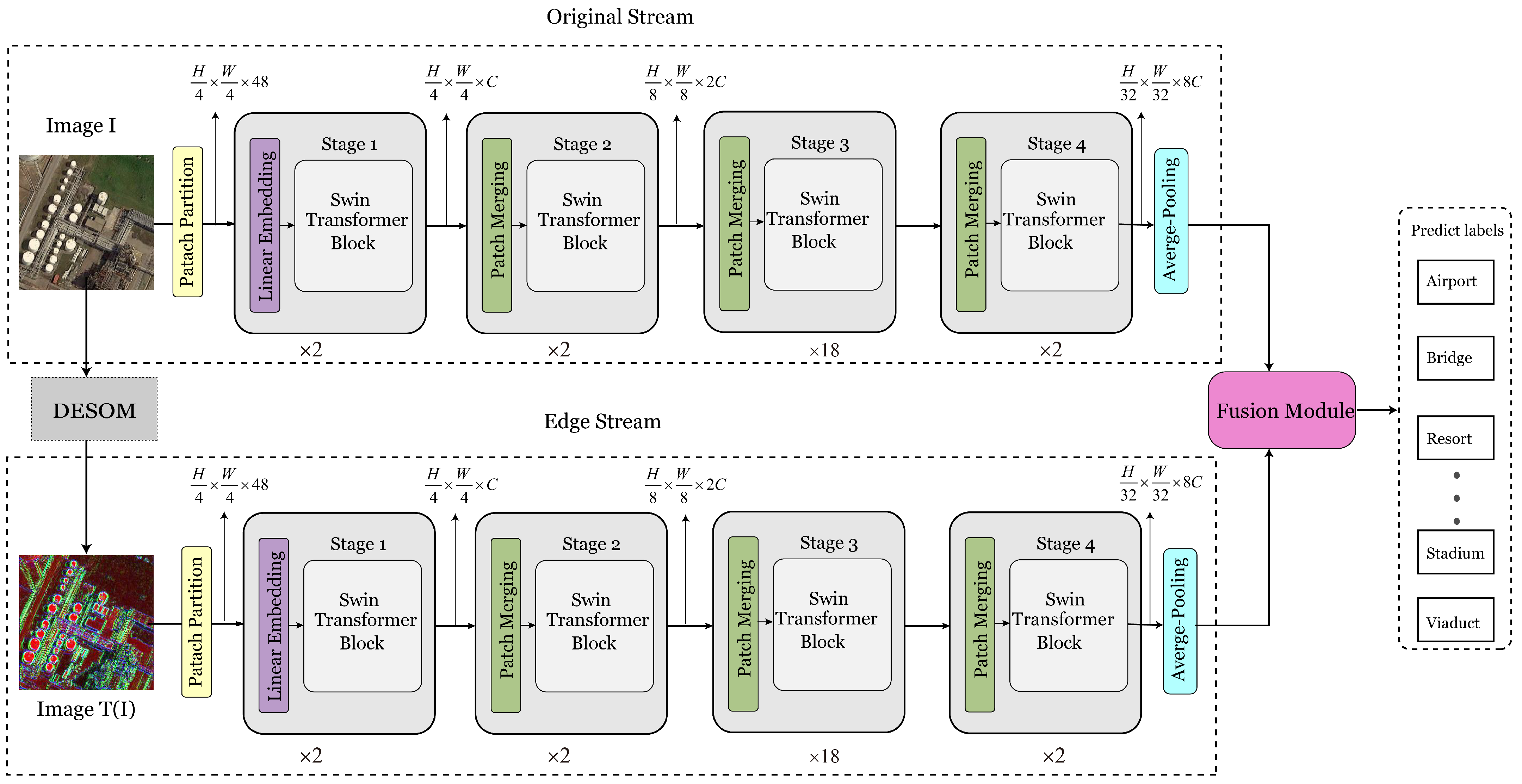
- A two-stream swin transformer network (TSTNet) is designed for remote sensing image classification. The first stream is in charge of extracting the original image features while the second stream is in charge of extracting the edge information.
- (2)
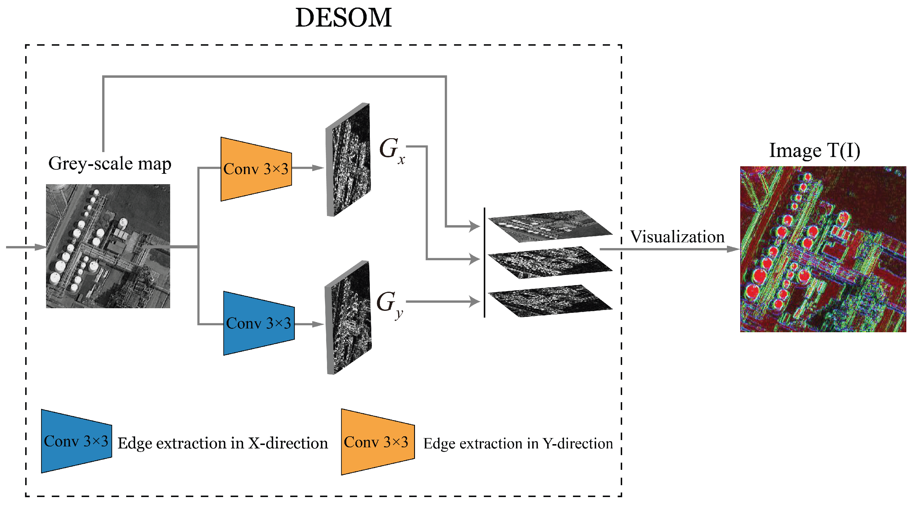
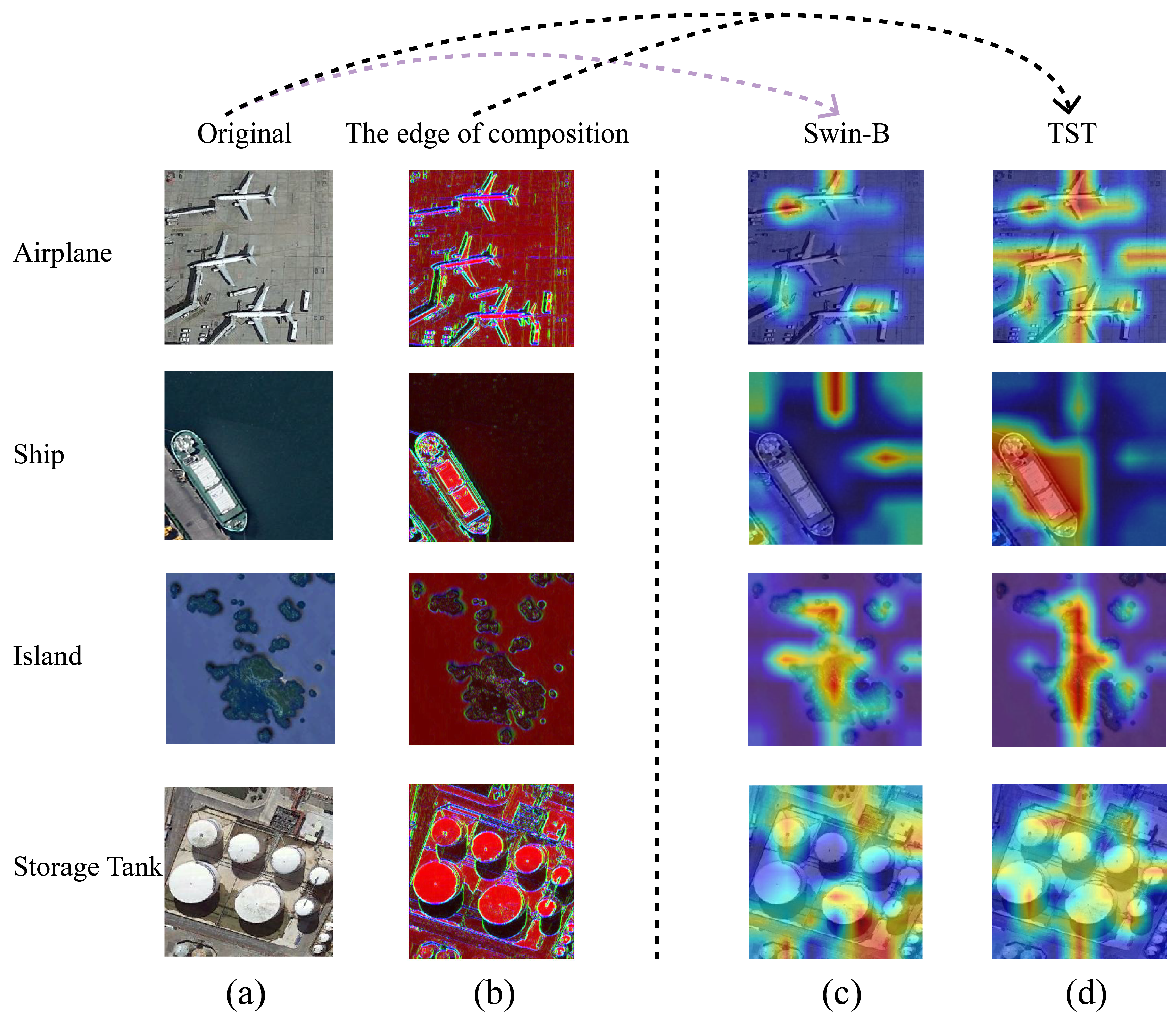
- To extract more powerful edge features for the remote sensing images, a novel differentiable edge Sobel operator module (DESOM) is proposed in the second stream.
- (3)
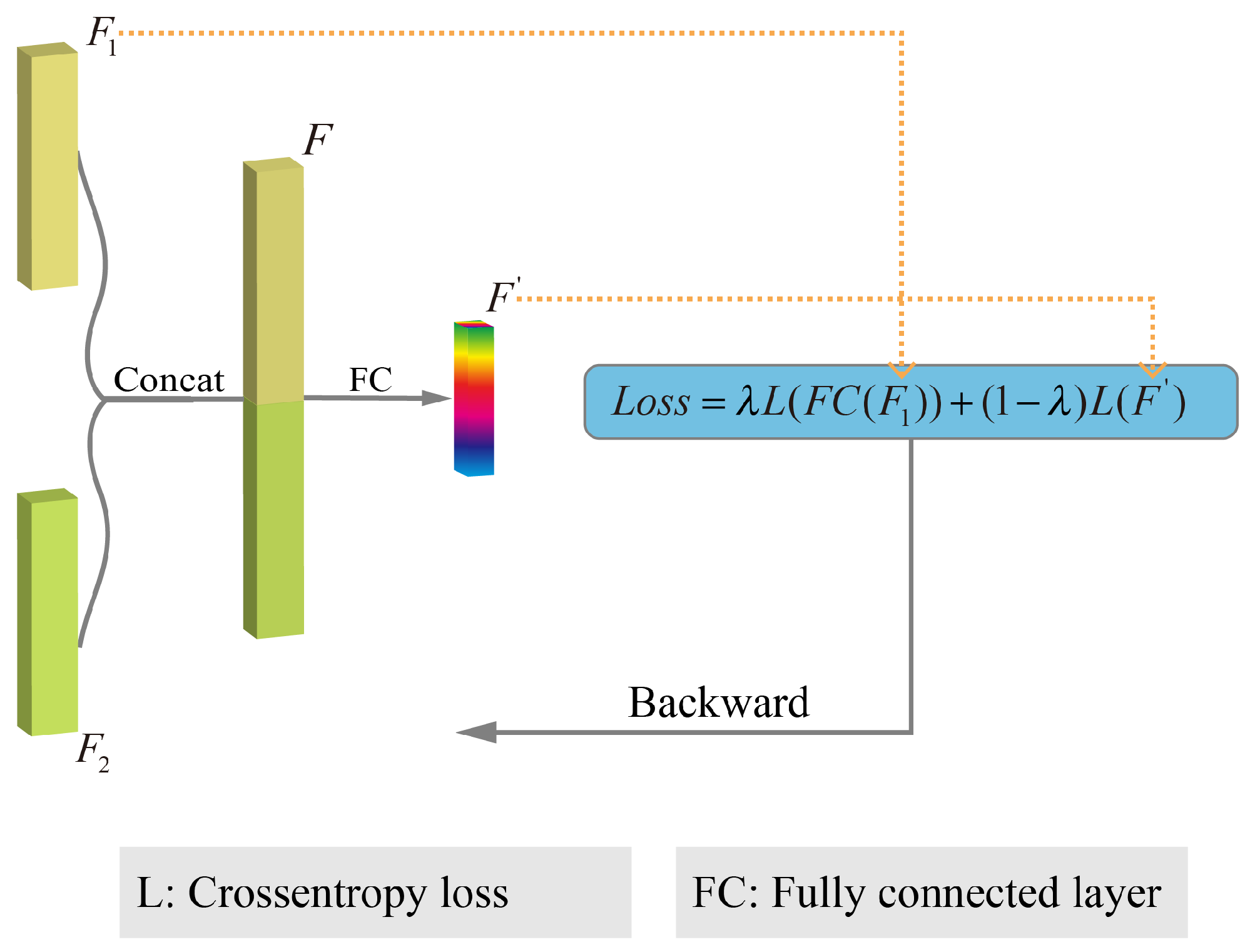
- We have designed a weighted feature fusion module to enable the edge information and the original image information to be fused effectively to boost the classification performance.
2. Related Works
2.1. Hand-Crafted Features
2.2. CNNs in Remote Sensing Image Classification
2.3. Transformer in Vision
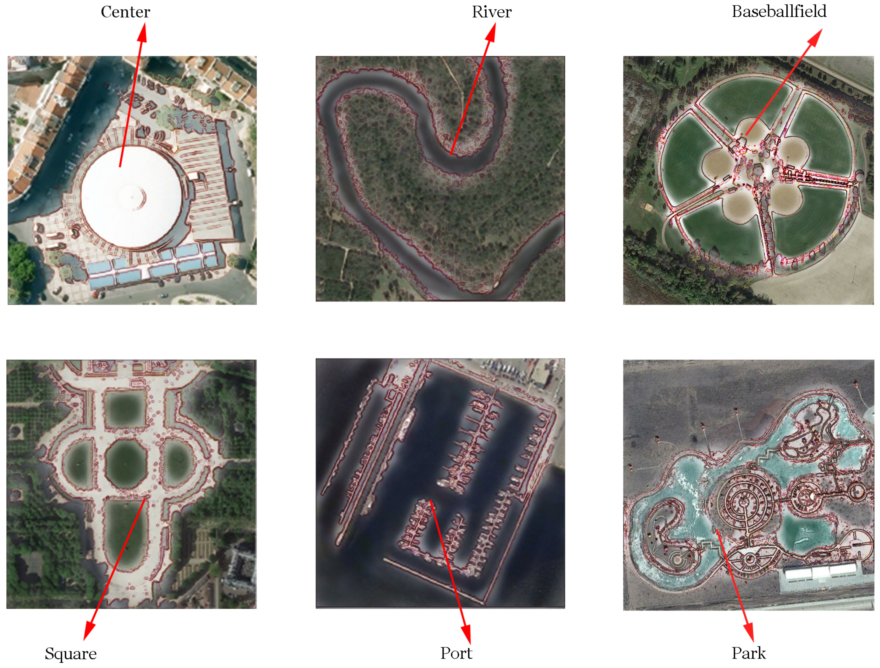
2.4. Application of Edge Information in Remote Sensing
3. Proposed Method
3.1. Overall Framework
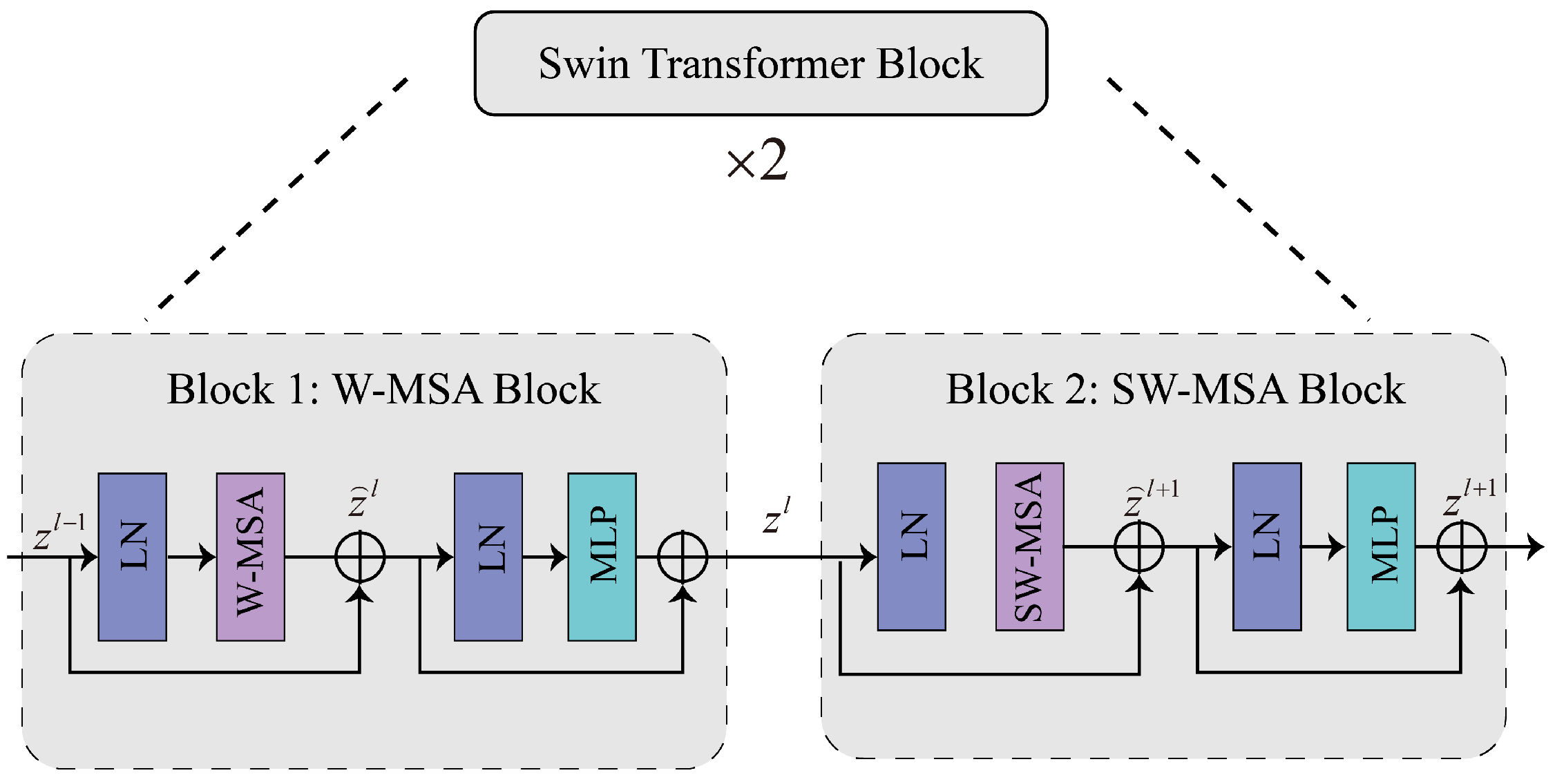
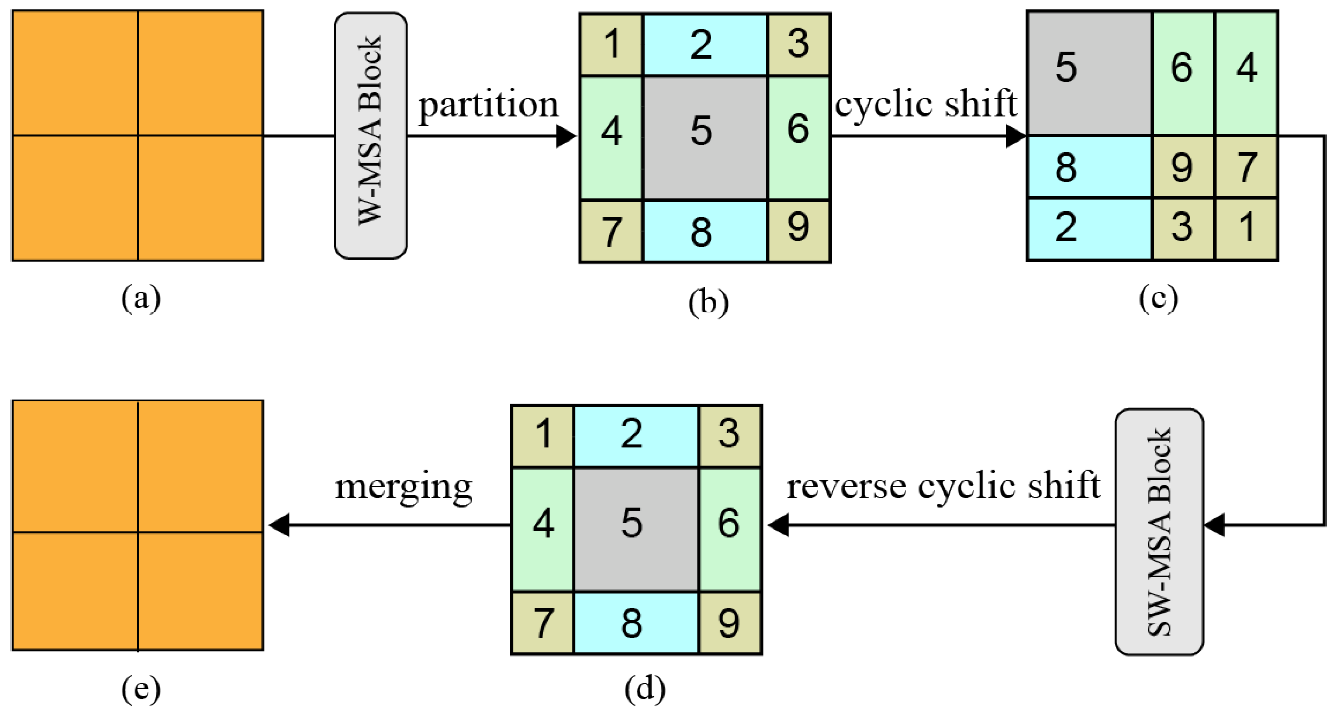
3.2. Backbone for Feature Extraction
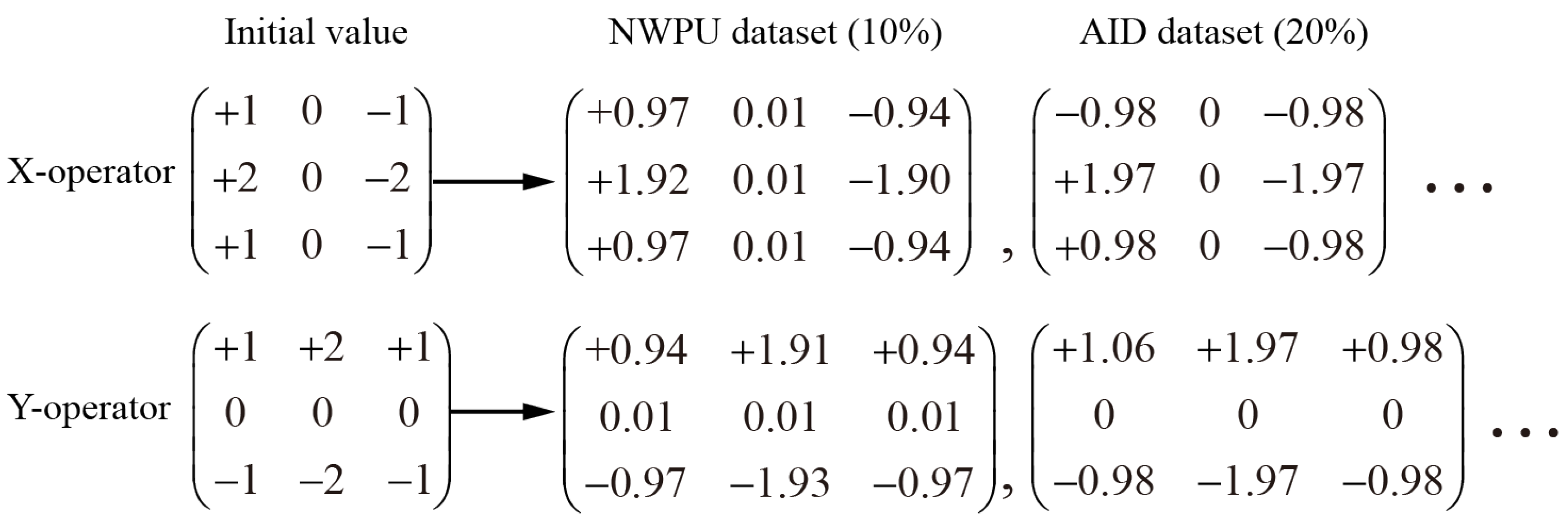
3.3. Differentiable Edge Sobel Operator Module
3.4. Feature Fusion
4. Experiments
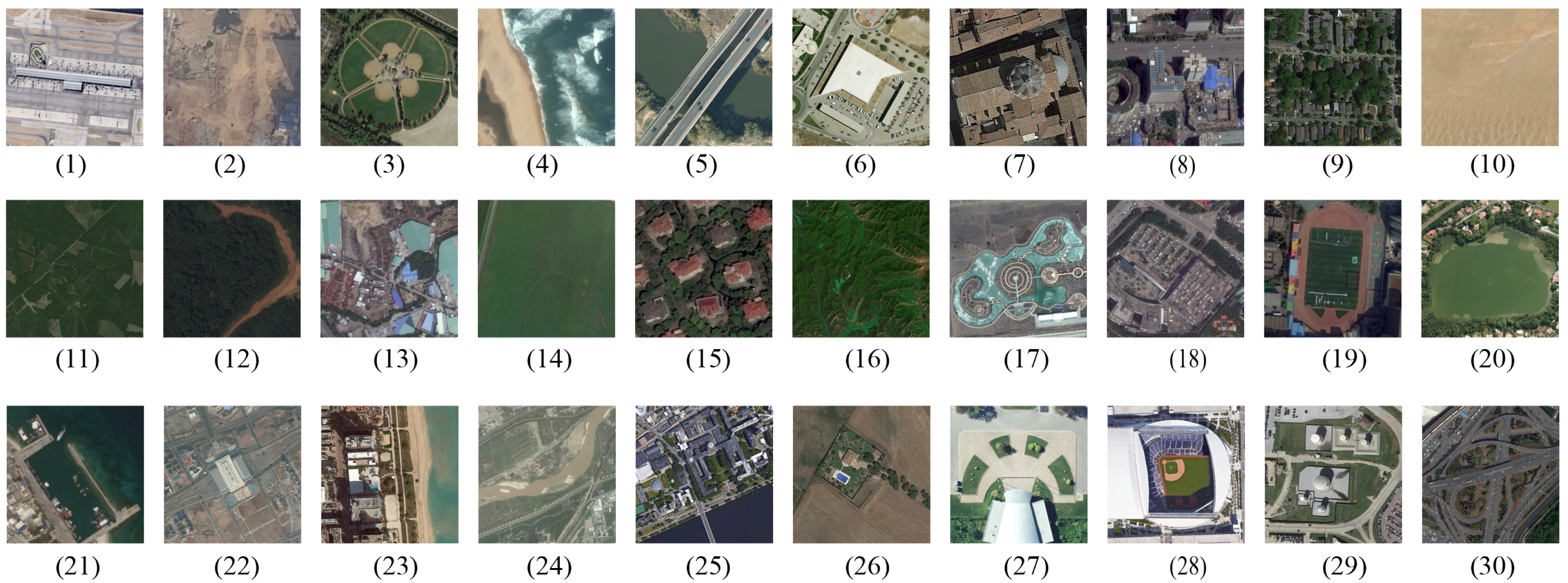
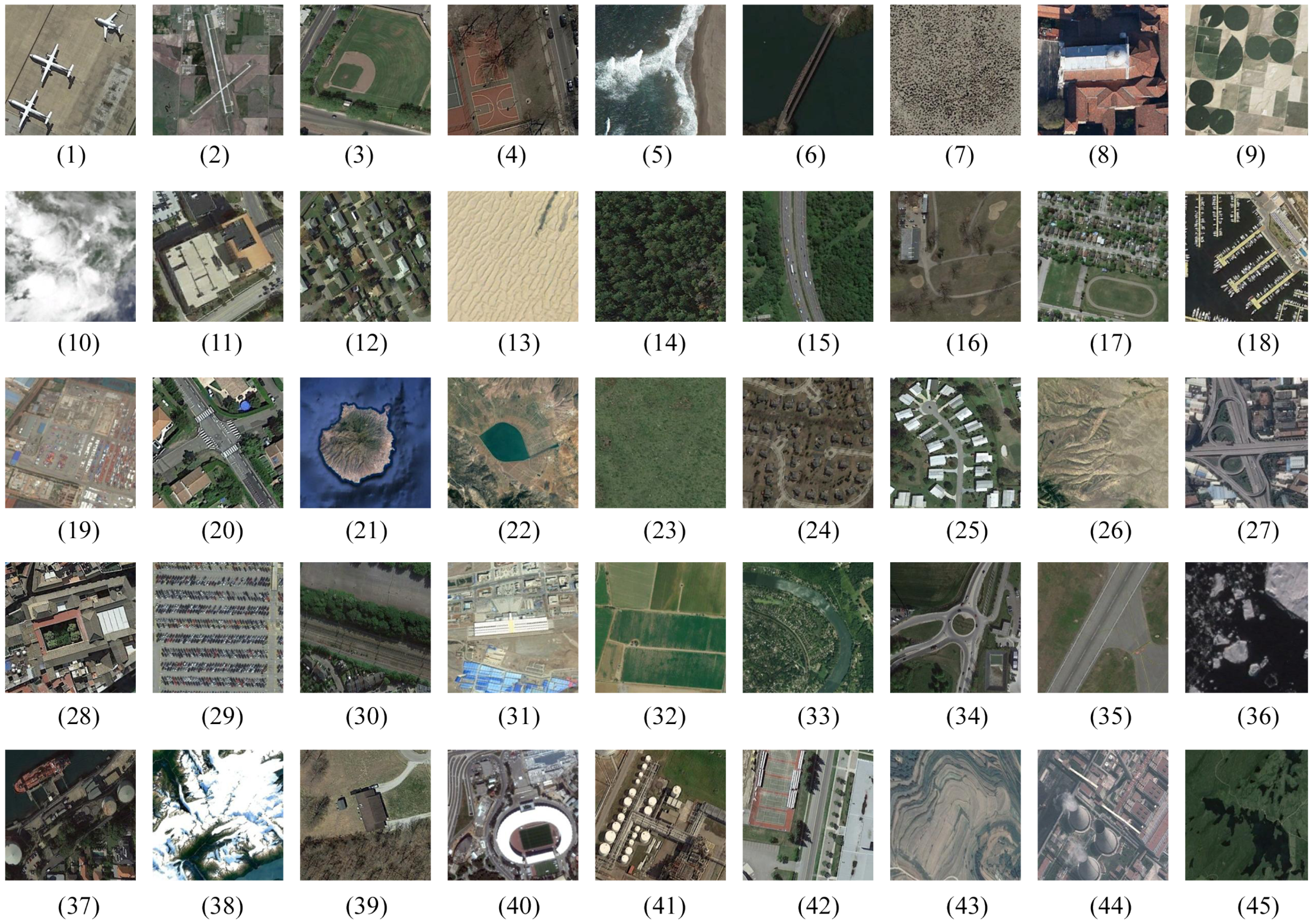
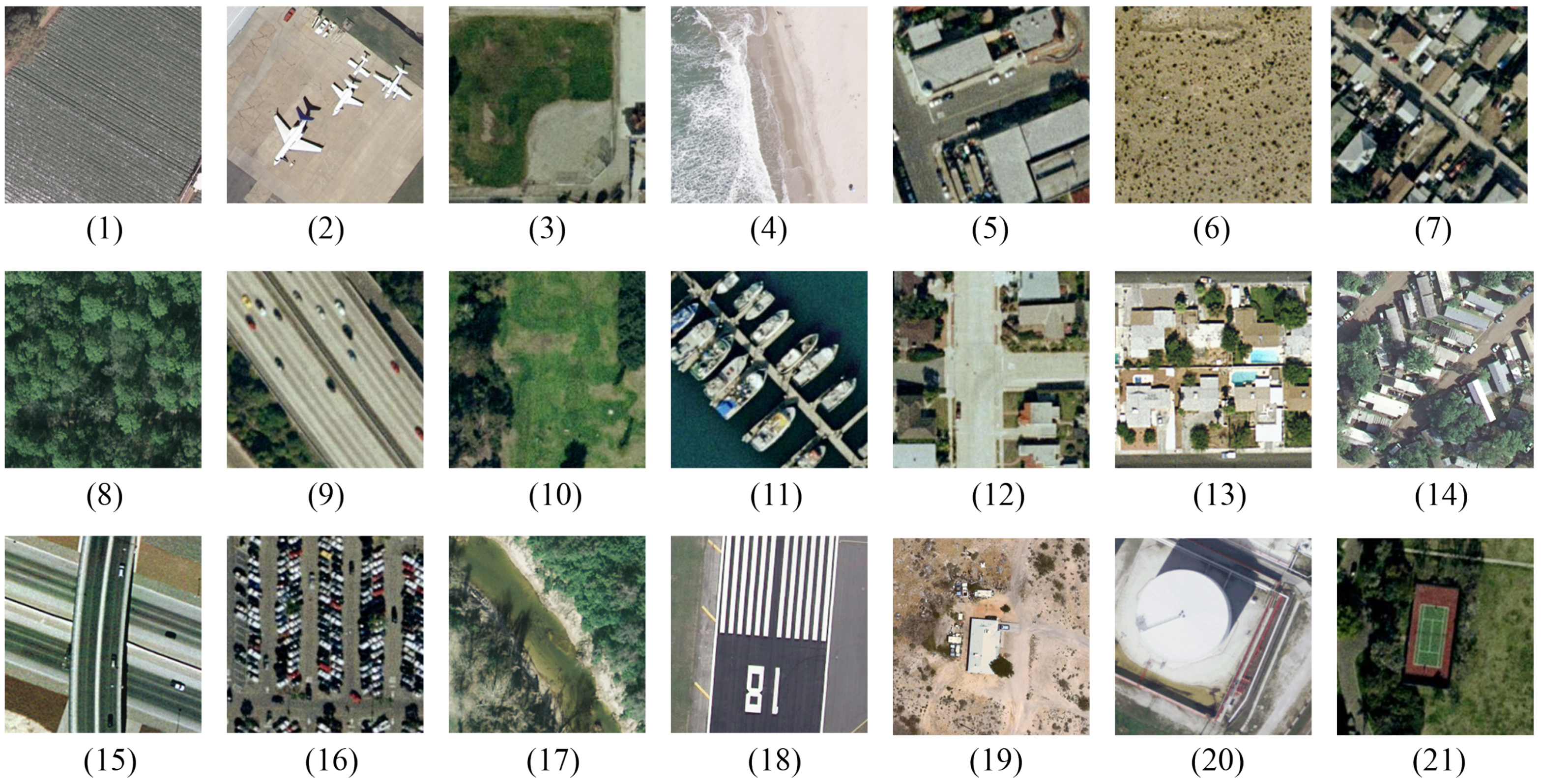
4.1. Datasets
4.2. Experimental Setup
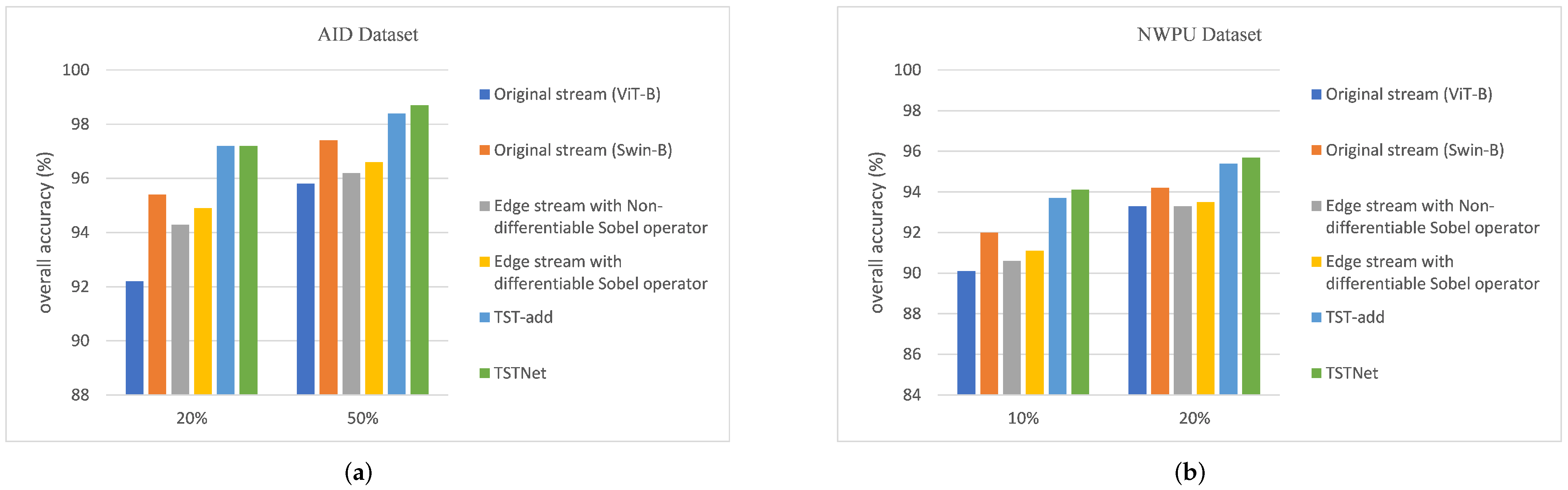
4.3. Ablation Study
- First, to demonstrate the good performance of Swin-B over ViT-B, we conducted experiments using a single-branch original stream which was either based on ViT-B or Swin-B.
- In addition, to demonstrate the effectiveness of DESOM, we compared the edge stream using Sobel operator with fixed values and edge stream with differentiable Sobel operator whose values can be learned adaptively.
- Finally, our proposed architecture (i.e., TSTNet) concatenates the features from the two branches directly and it has a weighted loss function which balances the contribution of the two streams. To check the effectiveness of the loss function, we replaced the concatenation operation with a simple add operation. This baseline is named TST-add and uses a simple cross entropy loss treating the two streams equivalently.
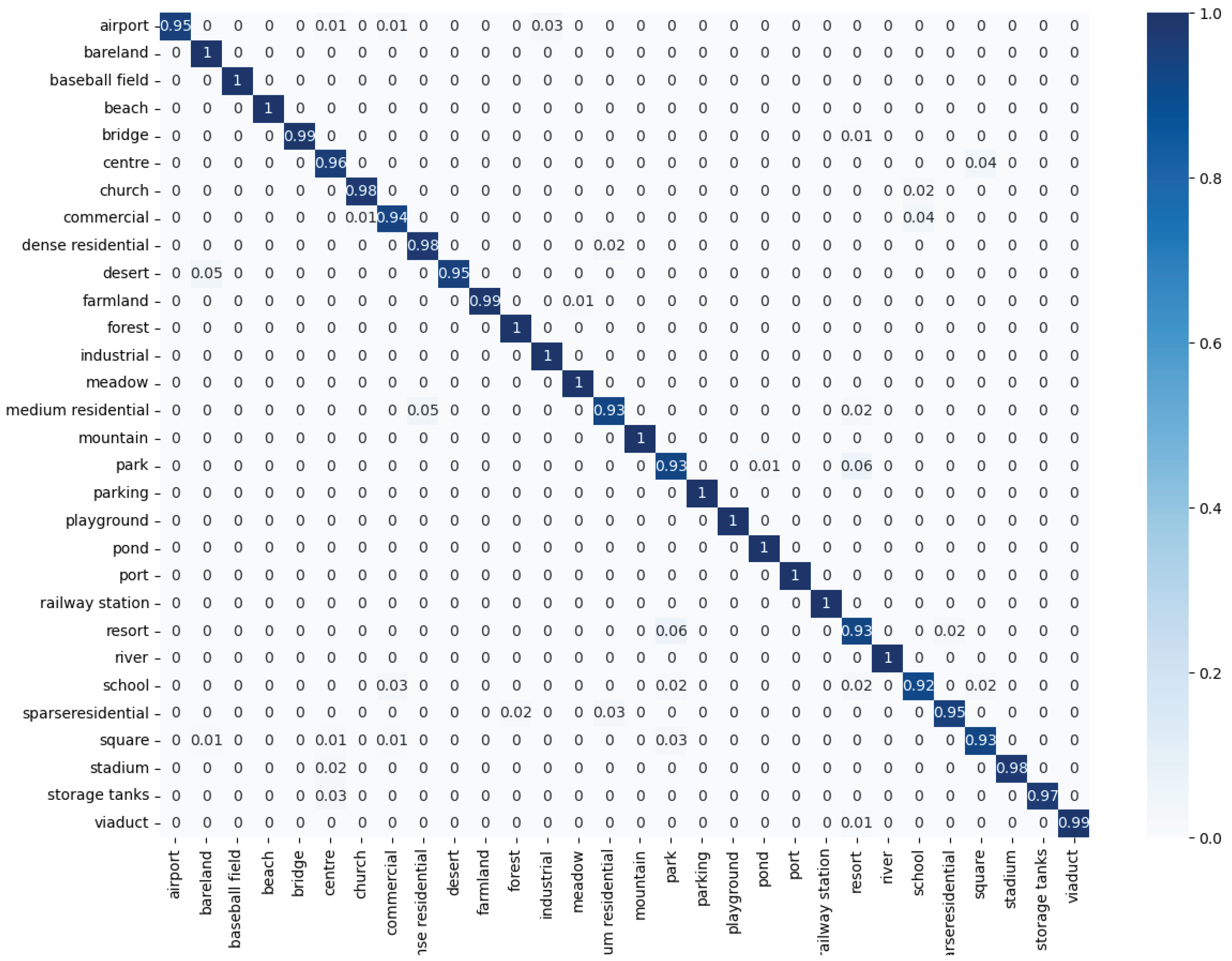
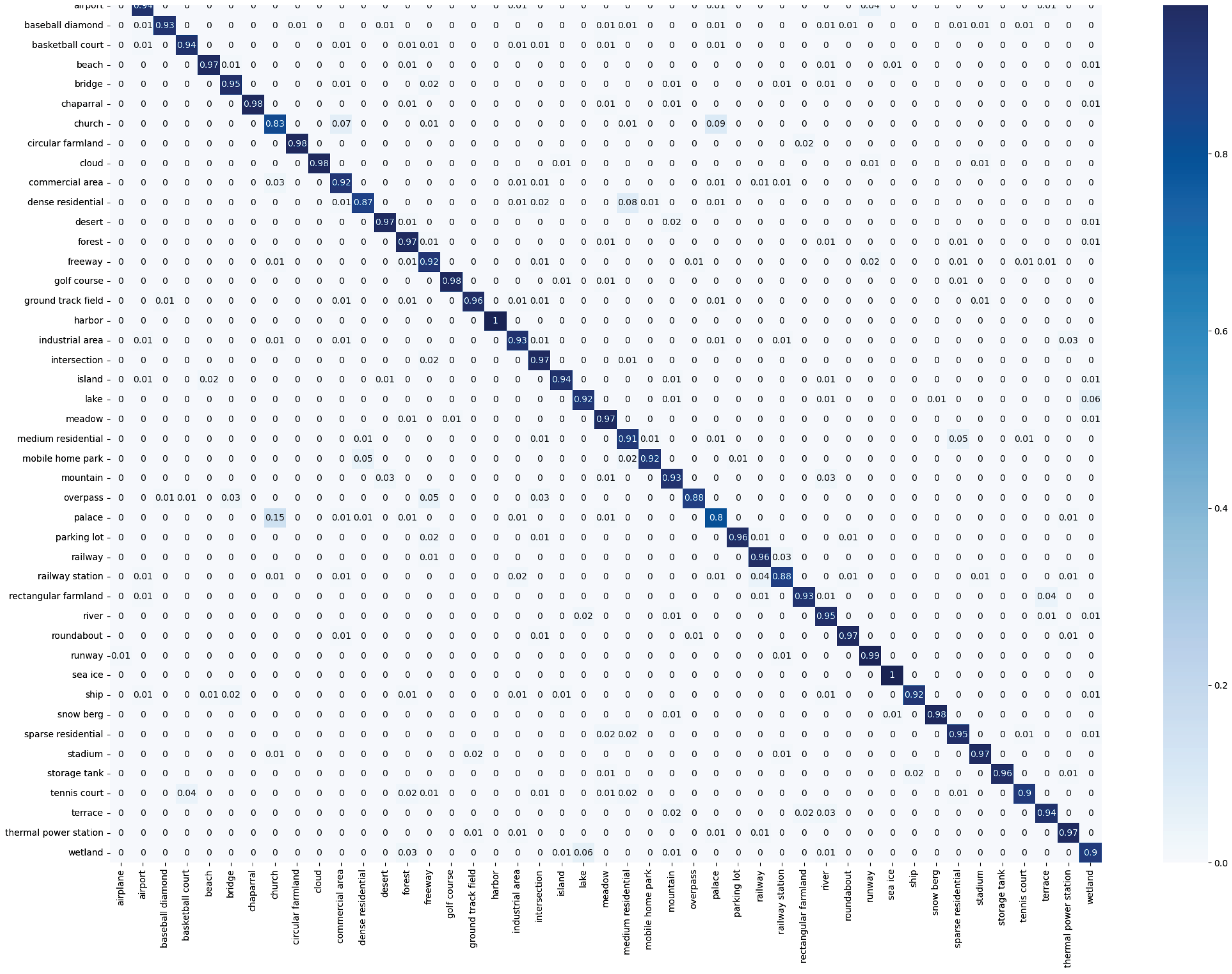
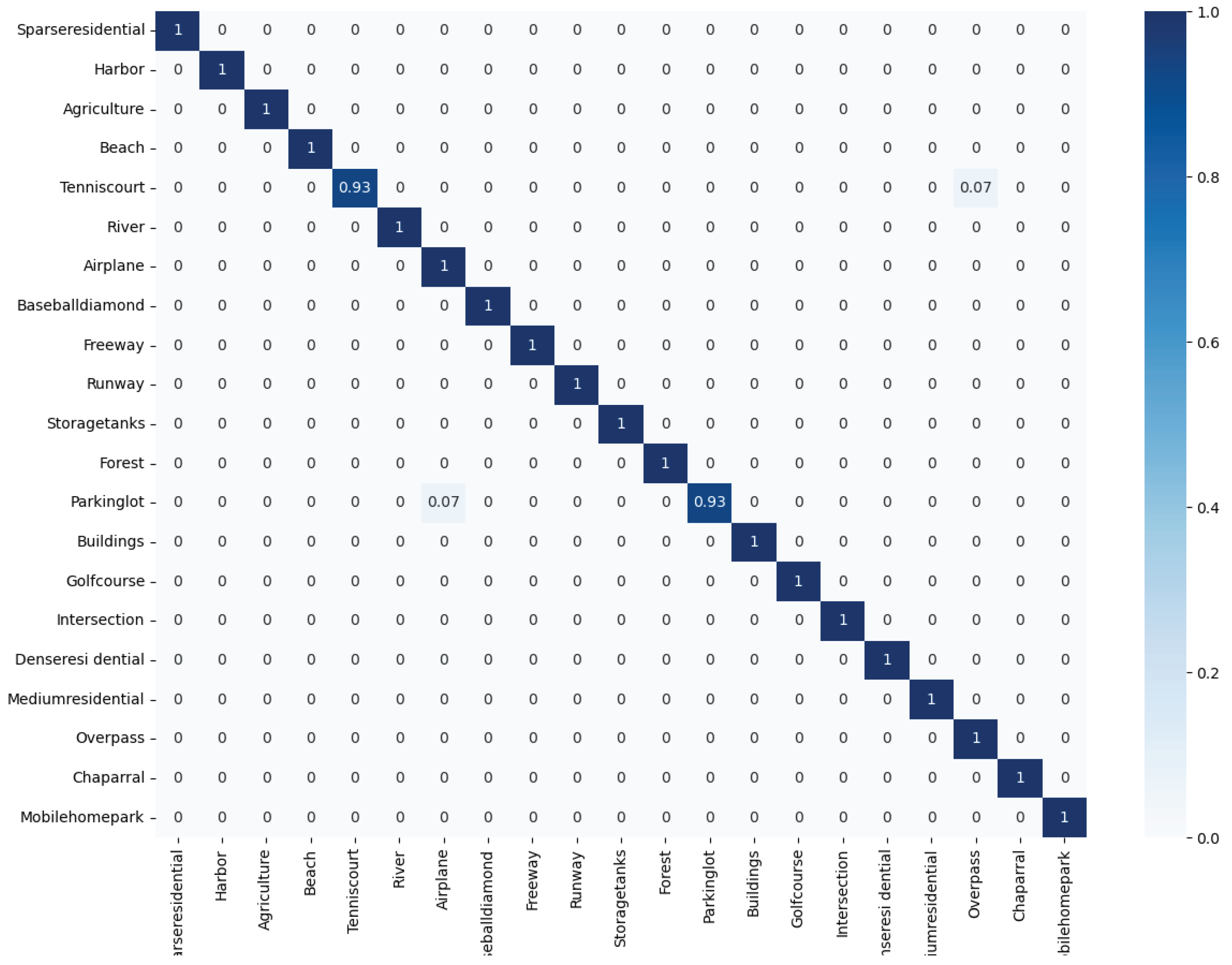
4.4. Experimental Results
- Compared with the Inception-v3-CapsNet which is based on Inception-v3, the overall accuracy is increased by 3.41% and 2.47% using our TSTNet.
- Our TSTNet is 1.7% higher than the CNN-based method KFBNet (DenseNet-121) for the 10% training ratio. In the case of the 20% training ratio, it is 1.05% higher.
- Currently, there are also many vision transformer (ViT)-based remote sensing image classification methods that further improve the upper limit of classification performance. The overall accuracy of our TSTNet is 1.66% higher than the TRS method with 10% training ratio and 0.22% higher with 20% training ratio.
- The overall accuracy of our TSTNet is 94.08% and 95.70% with the training ratio of 10% and 20%, and it outperforms the state-of-the-art baselines, such as CNN-based method, by a large margin. This is especially true for the small training ratio.
- Under the 10% training ratio, our TSTNet increases the acuracy by 2.99% and 2.17% compared with ACNet and Xu’s method. Under the 20% training ratio, 3.28% and 1.27% performance improvement is achieved.
- The performance of our TSTNet also outperforms the ViT-based method. Under the 10% training ratio, TSTNet improves 0.18% and 1.02% compared with CTNet (mobileNetv2) and TRS. Under the 20% training ratio, the improvement is 0.30% and 0.14%.
4.5. Running Time and Parameters of the TSTNet
5. Discussion
5.1. Study the Invariance of Transformations
5.2. Selection of Edge Detection Operator
6. Conclusions
Author Contributions
Funding
Data Availability Statement
Acknowledgments
Conflicts of Interest
References
- Zheng, X.; Gong, T.; Li, X.; Lu, X. Generalized Scene Classification From Small-Scale Datasets with Multitask Learning. IEEE Trans. Geosci. Remote Sens. 2021, 60, 5609311. [Google Scholar] [CrossRef]
- Zheng, X.; Chen, X.; Lu, X.; Sun, B. Unsupervised change detection by cross-resolution difference learning. IEEE Trans. Geosci. Remote Sens. 2021, 60, 5606616. [Google Scholar] [CrossRef]
- Zheng, X.; Wang, B.; Du, X.; Lu, X. Mutual attention inception network for remote sensing visual question answering. IEEE Trans. Geosci. Remote Sens. 2021, 60, 5606514. [Google Scholar] [CrossRef]
- Ye, Y.; Bruzzone, L.; Shan, J.; Bovolo, F.; Zhu, Q. Fast and robust matching for multimodal remote sensing image registration. IEEE Trans. Geosci. Remote Sens. 2019, 57, 9059–9070. [Google Scholar] [CrossRef] [Green Version]
- Zhou, L.; Ye, Y.; Tang, T.; Nan, K.; Qin, Y. Robust Matching for SAR and Optical Images Using Multiscale Convolutional Gradient Features. IEEE Geosci. Remote Sens. Lett. 2021, 19, 4017605. [Google Scholar] [CrossRef]
- Hu, Q.; Wu, W.; Xia, T.; Yu, Q.; Yang, P.; Li, Z.; Song, Q. Exploring the use of Google Earth imagery and object-based methods in land use/cover mapping. Remote Sens. 2013, 5, 6026–6042. [Google Scholar] [CrossRef] [Green Version]
- Gómez-Chova, L.; Tuia, D.; Moser, G.; Camps-Valls, G. Multimodal classification of remote sensing images: A review and future directions. Proc. IEEE 2015, 103, 1560–1584. [Google Scholar] [CrossRef]
- Longbotham, N.; Chaapel, C.; Bleiler, L.; Padwick, C.; Emery, W.J.; Pacifici, F. Very high resolution multiangle urban classification analysis. IEEE Trans. Geosci. Remote Sens. 2011, 50, 1155–1170. [Google Scholar] [CrossRef]
- Tayyebi, A.; Pijanowski, B.C.; Tayyebi, A.H. An urban growth boundary model using neural networks, GIS and radial parameterization: An application to Tehran, Iran. Landsc. Urban Plan. 2011, 100, 35–44. [Google Scholar] [CrossRef]
- Wang, Y.; Zhang, L.; Tong, X.; Zhang, L.; Zhang, Z.; Liu, H.; Xing, X.; Mathiopoulos, P.T. A three-layered graph-based learning approach for remote sensing image retrieval. IEEE Trans. Geosci. Remote Sens. 2016, 54, 6020–6034. [Google Scholar] [CrossRef]
- Yang, Y.; Newsam, S. Geographic image retrieval using local invariant features. IEEE Trans. Geosci. Remote Sens. 2012, 51, 818–832. [Google Scholar] [CrossRef]
- Huang, X.; Wen, D.; Li, J.; Qin, R. Multi-level monitoring of subtle urban changes for the megacities of China using high-resolution multi-view satellite imagery. Remote Sens. Environ. 2017, 196, 56–75. [Google Scholar] [CrossRef]
- Zhang, T.; Huang, X. Monitoring of urban impervious surfaces using time series of high-resolution remote sensing images in rapidly urbanized areas: A case study of Shenzhen. IEEE J. Sel. Top. Appl. Earth Obs. Remote Sens. 2018, 11, 2692–2708. [Google Scholar] [CrossRef]
- Ghazouani, F.; Farah, I.R.; Solaiman, B. A multi-level semantic scene interpretation strategy for change interpretation in remote sensing imagery. IEEE Trans. Geosci. Remote Sens. 2019, 57, 8775–8795. [Google Scholar] [CrossRef]
- Li, X.; Shao, G. Object-based urban vegetation mapping with high-resolution aerial photography as a single data source. Int. J. Remote Sens. 2013, 34, 771–789. [Google Scholar] [CrossRef]
- Mishra, N.B.; Crews, K.A. Mapping vegetation morphology types in a dry savanna ecosystem: Integrating hierarchical object-based image analysis with Random Forest. Int. J. Remote Sens. 2014, 35, 1175–1198. [Google Scholar] [CrossRef]
- Cheng, G.; Zhou, P.; Han, J. Learning rotation-invariant convolutional neural networks for object detection in VHR optical remote sensing images. IEEE Trans. Geosci. Remote Sens. 2016, 54, 7405–7415. [Google Scholar] [CrossRef]
- Li, Y.; Zhang, Y.; Huang, X.; Yuille, A.L. Deep networks under scene-level supervision for multi-class geospatial object detection from remote sensing images. ISPRS J. Photogramm. Remote Sens. 2018, 146, 182–196. [Google Scholar] [CrossRef]
- Cheng, G.; Han, J.; Zhou, P.; Xu, D. Learning rotation-invariant and fisher discriminative convolutional neural networks for object detection. IEEE Trans. Image Process. 2018, 28, 265–278. [Google Scholar] [CrossRef]
- Li, K.; Wan, G.; Cheng, G.; Meng, L.; Han, J. Object detection in optical remote sensing images: A survey and a new benchmark. ISPRS J. Photogramm. Remote Sens. 2020, 159, 296–307. [Google Scholar] [CrossRef]
- Li, K.; Cheng, G.; Bu, S.; You, X. Rotation-insensitive and context-augmented object detection in remote sensing images. IEEE Trans. Geosci. Remote Sens. 2017, 56, 2337–2348. [Google Scholar] [CrossRef]
- Cheng, G.; Zhou, P.; Han, J. Rifd-cnn: Rotation-invariant and fisher discriminative convolutional neural networks for object detection. In Proceedings of the IEEE Conference on Computer Vision and Pattern Recognition, Las Vegas, NV, USA, 27–30 June 2016; pp. 2884–2893. [Google Scholar]
- Cheng, G.; Han, J.; Guo, L.; Liu, T. Learning coarse-to-fine sparselets for efficient object detection and scene classification. In Proceedings of the IEEE Conference on Computer Vision and Pattern Recognition, Boston, MA, USA, 7–12 June 2015; pp. 1173–1181. [Google Scholar]
- Cheng, G.; Ma, C.; Zhou, P.; Yao, X.; Han, J. Scene classification of high resolution remote sensing images using convolutional neural networks. In Proceedings of the 2016 IEEE International Geoscience and Remote Sensing Symposium (IGARSS), Beijing, China, 10–15 July 2016; pp. 767–770. [Google Scholar]
- Zhou, W.; Shao, Z.; Cheng, Q. Deep feature representations for high-resolution remote sensing scene classification. In Proceedings of the 2016 4th International Workshop on Earth Observation and Remote Sensing Applications (EORSA), Guangzhou, China, 4–6 July 2016; pp. 338–342. [Google Scholar]
- Wang, Q.; Liu, S.; Chanussot, J.; Li, X. Scene classification with recurrent attention of VHR remote sensing images. IEEE Trans. Geosci. Remote Sens. 2018, 57, 1155–1167. [Google Scholar] [CrossRef]
- Dosovitskiy, A.; Beyer, L.; Kolesnikov, A.; Weissenborn, D.; Zhai, X.; Unterthiner, T.; Dehghani, M.; Minderer, M.; Heigold, G.; Gelly, S.; et al. An image is worth 16x16 words: Transformers for image recognition at scale. arXiv 2020, arXiv:2010.11929. [Google Scholar]
- Bazi, Y.; Bashmal, L.; Rahhal, M.M.A.; Dayil, R.A.; Ajlan, N.A. Vision transformers for remote sensing image classification. Remote Sens. 2021, 13, 516. [Google Scholar] [CrossRef]
- Deng, P.; Xu, K.; Huang, H. When CNNs Meet Vision Transformer: A Joint Framework for Remote Sensing Scene Classification. IEEE Geosci. Remote Sens. Lett. 2021, 19, 8020305. [Google Scholar] [CrossRef]
- Zhang, J.; Zhao, H.; Li, J. TRS: Transformers for Remote Sensing Scene Classification. Remote Sens. 2021, 13, 4143. [Google Scholar] [CrossRef]
- Liu, Z.; Lin, Y.; Cao, Y.; Hu, H.; Wei, Y.; Zhang, Z.; Lin, S.; Guo, B. Swin transformer: Hierarchical vision transformer using shifted windows. arXiv 2021, arXiv:2103.14030. [Google Scholar]
- Swain, M.J.; Ballard, D.H. Color indexing. Int. J. Comput. Vis. 1991, 7, 11–32. [Google Scholar] [CrossRef]
- Haralick, R.M.; Shanmugam, K.; Dinstein, I.H. Textural features for image classification. IEEE Trans. Syst. Man Cybern. 1973, 6, 610–621. [Google Scholar] [CrossRef] [Green Version]
- Oliva, A.; Torralba, A. Modeling the shape of the scene: A holistic representation of the spatial envelope. Int. J. Comput. Vis. 2001, 42, 145–175. [Google Scholar] [CrossRef]
- Lowe, D.G. Distinctive image features from scale-invariant keypoints. Int. J. Comput. Vis. 2004, 60, 91–110. [Google Scholar] [CrossRef]
- Dalal, N.; Triggs, B. Histograms of oriented gradients for human detection. In Proceedings of the 2005 IEEE Computer Society Conference on Computer Vision and Pattern Recognition (CVPR’05), San Diego, CA, USA, 20–25 June 2005; Volume 1, pp. 886–893. [Google Scholar]
- Krizhevsky, A.; Sutskever, I.; Hinton, G.E. Imagenet classification with deep convolutional neural networks. Adv. Neural Inf. Process. Syst. 2012, 25, 1097–1105. [Google Scholar] [CrossRef]
- Simonyan, K.; Zisserman, A. Very deep convolutional networks for large-scale image recognition. arXiv 2014, arXiv:1409.1556. [Google Scholar]
- He, K.; Zhang, X.; Ren, S.; Sun, J. Deep residual learning for image recognition. In Proceedings of the IEEE Conference on Computer Vision and Pattern Recognition, Las Vegas, NV, USA, 27–30 June 2016; pp. 770–778. [Google Scholar]
- Huang, G.; Liu, Z.; Van Der Maaten, L.; Weinberger, K.Q. Densely connected convolutional networks. In Proceedings of the IEEE Conference on Computer Vision and Pattern Recognition, Honolulu, HI, USA, 21–26 July 2017; pp. 4700–4708. [Google Scholar]
- Fan, R.; Wang, L.; Feng, R.; Zhu, Y. Attention based residual network for high-resolution remote sensing imagery scene classification. In Proceedings of the IGARSS 2019—2019 IEEE International Geoscience and Remote Sensing Symposium, Yokohama, Japan, 28 July–2 August 2019; pp. 1346–1349. [Google Scholar]
- Zhang, W.; Tang, P.; Zhao, L. Remote sensing image scene classification using CNN-CapsNet. Remote Sens. 2019, 11, 494. [Google Scholar] [CrossRef] [Green Version]
- Sun, H.; Li, S.; Zheng, X.; Lu, X. Remote sensing scene classification by gated bidirectional network. IEEE Trans. Geosci. Remote Sens. 2019, 58, 82–96. [Google Scholar] [CrossRef]
- Xu, C.; Zhu, G.; Shu, J. A Lightweight and Robust Lie Group-Convolutional Neural Networks Joint Representation for Remote Sensing Scene Classification. IEEE Trans. Geosci. Remote Sens. 2021, 60, 5501415. [Google Scholar] [CrossRef]
- Touvron, H.; Cord, M.; Douze, M.; Massa, F.; Sablayrolles, A.; Jégou, H. Training data-efficient image transformers & distillation through attention. In Proceedings of the International Conference on Machine Learning, Virtual, 13–15 April 2021; pp. 10347–10357. [Google Scholar]
- Li, W.; Cao, D.; Peng, Y.; Yang, C. MSNet: A Multi-Stream Fusion Network for Remote Sensing Spatiotemporal Fusion Based on Transformer and Convolution. Remote Sens. 2021, 13, 3724. [Google Scholar] [CrossRef]
- Xu, Z.; Zhang, W.; Zhang, T.; Yang, Z.; Li, J. Efficient Transformer for Remote Sensing Image Segmentation. Remote Sens. 2021, 13, 3585. [Google Scholar] [CrossRef]
- He, C.; He, B.; Yin, X.; Wang, W.; Liao, M. Relationship prior and adaptive knowledge mimic based compressed deep network for aerial scene classification. IEEE Access 2019, 7, 137080–137089. [Google Scholar] [CrossRef]
- He, C.; Li, S.; Xiong, D.; Fang, P.; Liao, M. Remote sensing image semantic segmentation based on edge information guidance. Remote Sens. 2020, 12, 1501. [Google Scholar] [CrossRef]
- Xia, G.S.; Hu, J.; Hu, F.; Shi, B.; Bai, X.; Zhong, Y.; Zhang, L.; Lu, X. AID: A benchmark data set for performance evaluation of aerial scene classification. IEEE Trans. Geosci. Remote Sens. 2017, 55, 3965–3981. [Google Scholar] [CrossRef] [Green Version]
- Cheng, G.; Li, Z.; Yao, X.; Guo, L.; Wei, Z. Remote sensing image scene classification using bag of convolutional features. IEEE Geosci. Remote Sens. Lett. 2017, 14, 1735–1739. [Google Scholar] [CrossRef]
- Yang, Y.; Newsam, S. Bag-of-visual-words and spatial extensions for land-use classification. In Proceedings of the 18th SIGSPATIAL International Conference on Advances in Geographic Information Systems, San Jose, CA, USA, 2–5 November 2010; pp. 270–279. [Google Scholar]
- Bazi, Y.; Al Rahhal, M.M.; Alhichri, H.; Alajlan, N. Simple yet effective fine-tuning of deep CNNs using an auxiliary classification loss for remote sensing scene classification. Remote Sens. 2019, 11, 2908. [Google Scholar] [CrossRef] [Green Version]
- Tang, X.; Ma, Q.; Zhang, X.; Liu, F.; Ma, J.; Jiao, L. Attention consistent network for remote sensing scene classification. IEEE J. Sel. Top. Appl. Earth Obs. Remote Sens. 2021, 14, 2030–2045. [Google Scholar] [CrossRef]
- Li, F.; Feng, R.; Han, W.; Wang, L. High-resolution remote sensing image scene classification via key filter bank based on convolutional neural network. IEEE Trans. Geosci. Remote Sens. 2020, 58, 8077–8092. [Google Scholar] [CrossRef]
- Wang, X.; Wang, S.; Ning, C.; Zhou, H. Enhanced feature pyramid network with deep semantic embedding for remote sensing scene classification. IEEE Trans. Geosci. Remote Sens. 2021, 59, 7918–7932. [Google Scholar] [CrossRef]
- Liu, M.; Jiao, L.; Liu, X.; Li, L.; Liu, F.; Yang, S. C-CNN: Contourlet convolutional neural networks. IEEE Trans. Neural Netw. Learn. Syst. 2020, 32, 2636–2649. [Google Scholar] [CrossRef]
- Zhao, Z.; Luo, Z.; Li, J.; Chen, C.; Piao, Y. When self-supervised learning meets scene classification: Remote sensing scene classification based on a multitask learning framework. Remote Sens. 2020, 12, 3276. [Google Scholar] [CrossRef]
- Bi, Q.; Zhang, H.; Qin, K. Multi-scale stacking attention pooling for remote sensing scene classification. Neurocomputing 2021, 436, 147–161. [Google Scholar] [CrossRef]
- Bi, Q.; Qin, K.; Zhang, H.; Xie, J.; Li, Z.; Xu, K. APDC-Net: Attention pooling-based convolutional network for aerial scene classification. IEEE Geosci. Remote Sens. Lett. 2019, 17, 1603–1607. [Google Scholar] [CrossRef]
- Liu, Y.; Zhong, Y.; Fei, F.; Zhu, Q.; Qin, Q. Scene classification based on a deep random-scale stretched convolutional neural network. Remote Sens. 2018, 10, 444. [Google Scholar] [CrossRef] [Green Version]
- Canny, J. A computational approach to edge detection. IEEE Trans. Pattern Anal. Mach. Intell. 1986, 6, 679–698. [Google Scholar] [CrossRef]


| Method Type | Method | 20% Train Ratio | 50% Train Ratio |
|---|---|---|---|
| △ | VGGNet [50] | 86.59 ± 0.29 | 89.64 ± 0.36 |
| GoogleNet [50] | 83.44 ± 0.40 | 86.39 ± 0.55 | |
| ARCNet-VGG16 [26] | 88.75 ± 0.40 | 93.10 ± 0.55 | |
| EfficientNet-B0-aux [53] | 93.96 ± 0.11 | − | |
| EfficientNet-B3-aux [53] | 94.19 ± 0.15 | − | |
| GBNet [43] | 90.16 ± 0.24 | 93.72 ± 0.34 | |
| GBNet+global feature [43] | 92.20 ± 0.23 | 95.48 ± 0.12 | |
| Inception-v3-CapsNet [42] | 93.79 ± 0.13 | 96.32 ± 0.12 | |
| ACNet [54] | 93.33 ± 0.29 | 95.38 ± 0.29 | |
| KFBNet(DenseNet-121) [55] | 95.50 ± 0.27 | 97.40 ± 0.10 | |
| EFPN-DSE-TDFF [56] | 94.02 ± 0.21 | 94.50 ± 0.30 | |
| Xu’s method [44] | 94.74 ± 0.23 | 97.65 ± 0.25 | |
| ◊ | V1621K[384 × 384] [28] | 95.86 ± 0.28 | − |
| V1621K[384 × 384] [pruning 50%] [28] | 94.27 ± 1.41 | − | |
| CTNet(ResNet34) [29] | 96.35 ± 0.13 | 97.56 ± 0.20 | |
| CTNet(MobileNetv2) [29] | 96.25 ± 0.10 | 97.70 ± 0.11 | |
| TRS [30] | 95.54 ± 0.18 | 98.48 ± 0.06 | |
| ⊙ | TSTNet(ours) | 97.20 ± 0.22 | 98.70 ± 0.12 |
| Method Type | Method | 10% Train Ratio | 20% Train Ratio |
|---|---|---|---|
| △ | VGGNet [50] | 76.69 ± 0.19 | 76.85 ± 0.18 |
| GoogleNet [50] | 76.19 ± 0.38 | 78.48 ± 0.26 | |
| EfficientNet-B0-aux [53] | 89.96 ± 0.27 | − | |
| EfficientNet-B3-aux [53] | 91.08 ± 0.14 | − | |
| Contourlet CNN [57] | 85.93 ± 0.51 | 89.57 ± 0.45 | |
| ResNeXt-101+MTL [58] | 91.91 ± 0.18 | 94.21 ± 0.15 | |
| VGGMS2AP [59] | 92.27 ± 0.21 | 93.91 ± 0.15 | |
| Inception-v3-CapsNet [42] | 89.03 ± 0.21 | 92.60 ± 0.11 | |
| KFBNet(DenseNet-121) [55] | 93.08 ± 0.14 | 95.11 ± 0.10 | |
| ACNet [54] | 91.09 ± 0.13 | 92.42 ± 0.16 | |
| Xu’s method [44] | 91.91 ± 0.15 | 94.43 ± 0.16 | |
| ◊ | V1621K[384 × 384] [28] | 93.83 ± 0.46 | − |
| V1621K[384 × 384] [pruning 50%] [28] | 93.05 ± 0.46 | − | |
| CTNet(ResNet34) [29] | 93.86 ± 0.22 | 95.49 ± 0.12 | |
| CTNet(MobileNetv2) [29] | 93.90 ± 0.14 | 95.40 ± 0.15 | |
| TRS [30] | 93.06 ± 0.11 | 95.56 ± 0.20 | |
| ⊙ | TSTNet(ours) | 94.08 ± 0.24 | 95.70 ± 0.10 |
| Method Type | Method | 50% Train Ratio | 80% Train Ratio |
|---|---|---|---|
| △ | VGGNet [50] | 94.14 ± 0.69 | 95.21 ± 1.20 |
| GoogleNet [50] | 92.70 ± 0.60 | 94.31 ± 0.89 | |
| APDCNet [60] | 95.01 ± 0.43 | 97.05 ± 0.43 | |
| SRSCNN [61] | 97.88 ± 0.31 | 98.13 ± 0.33 | |
| EfficientNet-B0-aux [53] | 98.01 ± 0.45 | − | |
| EfficientNet-B3-aux [53] | 98.22 ± 0.49 | − | |
| Contourlet CNN [57] | − | 98.97 ± 0.21 | |
| VGG-16-CapsNet [42] | 98.81 ± 0.22 | 95.33 ± 0.18 | |
| Inception-v3-CapsNet [42] | 97.59 ± 0.16 | 99.05 ± 0.24 | |
| ACNet [54] | − | 99.76 ± 0.10 | |
| EFPN-DSE-TDFF [56] | 96.19 ± 0.13 | 99.14 ± 0.22 | |
| Xu’s method [44] | 98.61 ± 0.22 | 98.97 ± 0.31 | |
| ◊ | V1621K[384 × 384] [28] | 98.49 ± 0.43 | − |
| V1621K[384 × 384] [pruning 50%] [28] | 97.90 ± 0.10 | − | |
| TRS [30] | 98.76 ± 0.13 | 99.52 ± 0.17 | |
| ⊙ | TSTNet(ours) | 98.95 ± 0.24 | 99.64 ± 0.21 |
| Method | Parameters | FLOPs | Throughput (Image/s) | Acc. (NWPU 10%) |
|---|---|---|---|---|
| ViT-B | 86 M | 16.8 G | 540 | 90.1 |
| Swin-B | 87 M | 15.4 G | 589 | 92.0 |
| ViT-L | 304 M | 59.6 G | 160 | 91.3 |
| Swin-L | 197 M | 34.5 G | 270 | 93.1 |
| TSTNet | 173 M | 30.2 G | 320 | 94.1 |
| Transformation | Cosine Imilarity | Accuracy | Accuracy Difference |
|---|---|---|---|
| without rotation | - | 95.690 | - |
| rotation | 0.977 | 95.875 | +0.185 |
| rotation | 0.972 | 95.315 | −0.375 |
| rotation | 0.971 | 95.750 | +0.060 |
| totation | 0.965 | 95.147 | −0.543 |
| Transformation | Cosine Similarity | Accuracy | Accuracy Difference |
|---|---|---|---|
| without scale | - | 95.690 | - |
| scale 1.1× | 0.974 | 96.110 | +0.420 |
| scale 1.2× | 0.971 | 95.857 | +0.167 |
| scale 1.3× | 0.965 | 95.607 | −0.083 |
| scale 1.4× | 0.965 | 95.151 | −0.539 |
| Operator Type | Accuracy (NWPU 20%) |
|---|---|
| Canny * [62] | 95.427 |
| Prewitt | 95.483 |
| Roberts | 94.678 |
| Sobel | 95.691 |
Publisher’s Note: MDPI stays neutral with regard to jurisdictional claims in published maps and institutional affiliations. |
© 2022 by the authors. Licensee MDPI, Basel, Switzerland. This article is an open access article distributed under the terms and conditions of the Creative Commons Attribution (CC BY) license (https://creativecommons.org/licenses/by/4.0/).
Share and Cite
Hao, S.; Wu, B.; Zhao, K.; Ye, Y.; Wang, W. Two-Stream Swin Transformer with Differentiable Sobel Operator for Remote Sensing Image Classification. Remote Sens. 2022, 14, 1507. https://doi.org/10.3390/rs14061507
Hao S, Wu B, Zhao K, Ye Y, Wang W. Two-Stream Swin Transformer with Differentiable Sobel Operator for Remote Sensing Image Classification. Remote Sensing. 2022; 14(6):1507. https://doi.org/10.3390/rs14061507
Chicago/Turabian StyleHao, Siyuan, Bin Wu, Kun Zhao, Yuanxin Ye, and Wei Wang. 2022. "Two-Stream Swin Transformer with Differentiable Sobel Operator for Remote Sensing Image Classification" Remote Sensing 14, no. 6: 1507. https://doi.org/10.3390/rs14061507