Article

Meta-Pixel-Driven Embeddable Discriminative Target and Background Dictionary Pair Learning for Hyperspectral Target Detection

1
School of Communication and Information Engineering, Chongqing University of Posts and Telecommunications, Chongqing 400065, China
2
Faculty of Information Technology, Macau University of Science and Technology, Taipa, Macau 999078, China
3
College of Computer Science, Chongqing University, Chongqing 401331, China
4
State Key Laboratory of Information Engineering in Surveying, Mapping and Remote Sensing, Wuhan University, Wuhan 430079, China
5
College of Electrical and Information Engineering, Hunan University, Changsha 410082, China
6
Faculty of Science and Technology, University of Macau, Macau 999078, China
*
Author to whom correspondence should be addressed.
Remote Sens. 2022, 14(3), 481; https://doi.org/10.3390/rs14030481
Submission received: 4 December 2021 / Revised: 19 January 2022 / Accepted: 19 January 2022 / Published: 20 January 2022
(This article belongs to the Special Issue State-of-the-Art Remote Sensing Image Scene Classification)

Abstract

:
In hyperspectral target detection, the spectral high-dimensionality, variability, and heterogeneity will pose great challenges to the accurate characterizations of the target and background. To alleviate the problems, we propose a Meta-pixel-driven Embeddable Discriminative target and background Dictionary Pair (MEDDP) learning model by combining low-dimensional embeddable subspace projection and the discriminative target and background dictionary pair learning. In MEDDP, the meta-pixel set is built by taking the merits of homogeneous superpixel segmentation and the local manifold affinity structures, which can significantly reduce the influence of spectral variability and find the most typical and informative prototype spectral signature. Afterward, an embeddable discriminative dictionary pair learning model is established to learn a target and background dictionary pair based on the structural incoherent constraint with embeddable subspace projection. The proposed joint learning strategy can reduce the high-dimensional redundant information and simultaneously enhance the discrimination and compactness of the target and background dictionaries. The proposed MEDDP model is solved by an iterative and alternate optimization algorithm and applied with the meta-pixel-level target detection method. Experimental results on four benchmark HSI datasets indicate that the proposed method can consistently yield promising performance in comparison with some state-of-the-art target detectors.

1. Introduction

Hyperspectral remote sensing image has the characteristic of high spectral resolution, which carries rich and consecutive spectral information of the land-covers. The diagnostic spectral information can distinguish the subtle differences between different spatially adjacent ground objects [1,2,3]. As a result, HSI has unique advantages in detecting ground targets of interest. HSI target detection refers to the process of separating key target pixels from the non-target ones, i.e., background, which is committed to highlighting the targets and simultaneously suppressing the background.
In HSI target detection, the target to be detected usually exists in the form of pixel-level or even sub-pixel level in the image, due to the complex distribution and composition of the ground objects, limited spatial resolution, and the small number and size of the targets [4,5]. Therefore, HSI target detection is usually transformed into the problem of determining the existence of target information in testing pixels. Given its numerous superiorities, HSI target detection technology has been successfully applied in many fields, such as the geologic and mineral survey, future urban planning, and military reconnaissance [6,7]. From the viewpoint of pattern recognition, HSI target detection can be regarded as an unbalanced binary classification problem with a large volume of background pixels and a low existence probability of target pixels. The basic idea is to strengthen the divisibility of the target and background with the guidance of known target prior spectra via spectral decomposition, spectral matching, or hypothesis test [7]. Some classical models, such as the Constrained Energy Minimization (CEM) [8], Adaptive Coherence Estimator (ACE) [9], and Spectral Matched Filter (SMF) [10], are usually served as the benchmarks.
In recent years, numerous advanced machine learning technologies, such as the sparse and low-rank modeling methods, have been successfully applied in a wide range of HSI processing applications, such as the HSI classification [11,12,13,14,15], unmixing [16,17], and target detection [18,19,20]. In a sparse representation-based target detector (SRD), the test pixel is represented or reconstructed by an over-complete dictionary composed of the background dictionary and known prior target spectra. The detection is then conducted by examining which sub-dictionary, i.e., background or target, yields a smaller representation residual [18]. Moreover, Zhang et al. suggested a sparse representation-based binary hypothesis (SRBBH) target detector, with the basic hypothesis that the testing pixels will be better reconstructed by the background dictionary when the target is absent [19]. By contrast, it will have a higher probability that the testing pixels can be more accurately reconstructed by the background and target combined dictionary when the target exists. Zhu et al. advocated a novel binary-class collaborative representation-based HSI target detector (BCRD) by assuming that the target pixels could be precisely represented by a collaborative representation of the pixels in the image [20]. To make better use of the distinct representation ability of the sparse and collaborative representation methods, a combined sparse and collaborative representation method has been proposed by taking the merits of both collaborative and sparse representations [21]. In addition, a sparse and dense hybrid representation-based HSI target detection method was presented, which can take full advantage of the structural prior information between the target and background for improved detection performance [22]. The key assumption for the above representation learning-based target detection methods is that the semantically similar HSI pixels will cluster and fall into a linear subspace.
In HSI target detection, the key problem is how to accurately characterize and estimate the target and background [4,8,23]. For example, some famous Gaussian-based target detectors, e.g., matched filter and normalized matched filter, depending on the unknown covariance matrix of the background around the test pixel, whose entries should be properly estimated [5]. Normally, the background can be characterized by some background pixels selected from the HSI scene. However, the background dictionary constructed in such a way might be contaminated by target information and failed to consider its discrimination in correspondence to the target prior information. Also, too many background pixels will increase the computational burden and make the problem more unbalanced. Chen et al. argued that using a local adaptive scheme-based sliding dual-window for background dictionary construction can generally achieve promising detection performance than using a global dictionary constructed by some background samples [18,24]. To separate a pure background dictionary, a sparse and low-rank matrix decomposition-based background dictionary construction method has recently been presented based on the robust principal component analysis (RPCA), which assumes that the background dictionary has a low-rank property and can be separated from the observed HSI by matrix decomposition [4]. However, little attention has been paid to the discrimination between the background and target dictionaries. Strengthening the discrimination between the target and background dictionaries can lead to better detection performance. Following the idea, a structural incoherent background and target dictionaries (SIBTD) learning method has been developed for HSI target detection [8]. In SIBTD, the structural incoherence constraint is introduced to enhance the discrimination between the target and background dictionaries. Nevertheless, due to the high dimensionality and heterogeneity of the spectra, these methods will also suffer from the problem of spectral variability. Therefore, the accurate, discriminative, and compact characterization issues of the target and background need to be resolved. As shown in Figure 1, this paper aims to handle the challenges by learning a discriminative target and background dictionary pair from the observed HSI data based on superpixel segmentation-derived meta-pixel with the guidance of target prior spectra and the structural incoherent regularization, in a jointly learned adaptive lower-dimensional embeddable subspace. In a nutshell, the main contributions are summarized below.
(1)
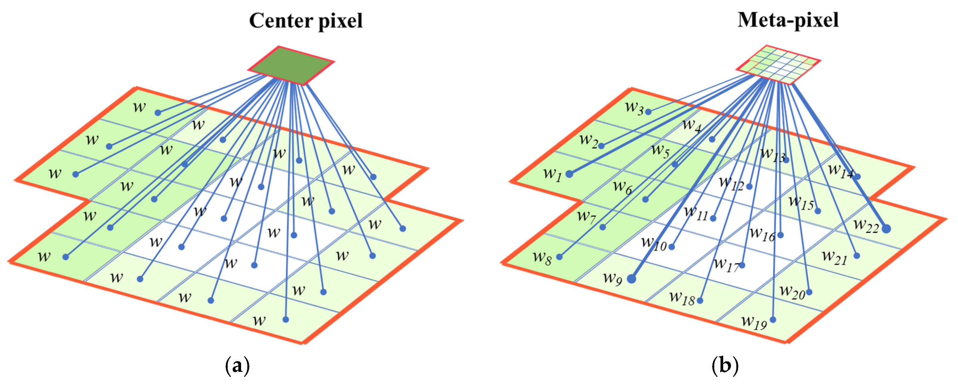
The meta-pixel set for HSI is defined by inheriting the merits of the homogeneous superpixel spectral property and the local manifold affinity structure, which can significantly reduce the influence of the spectral variability and find the most informative and prototype spectral signatures of HSI.
(2)
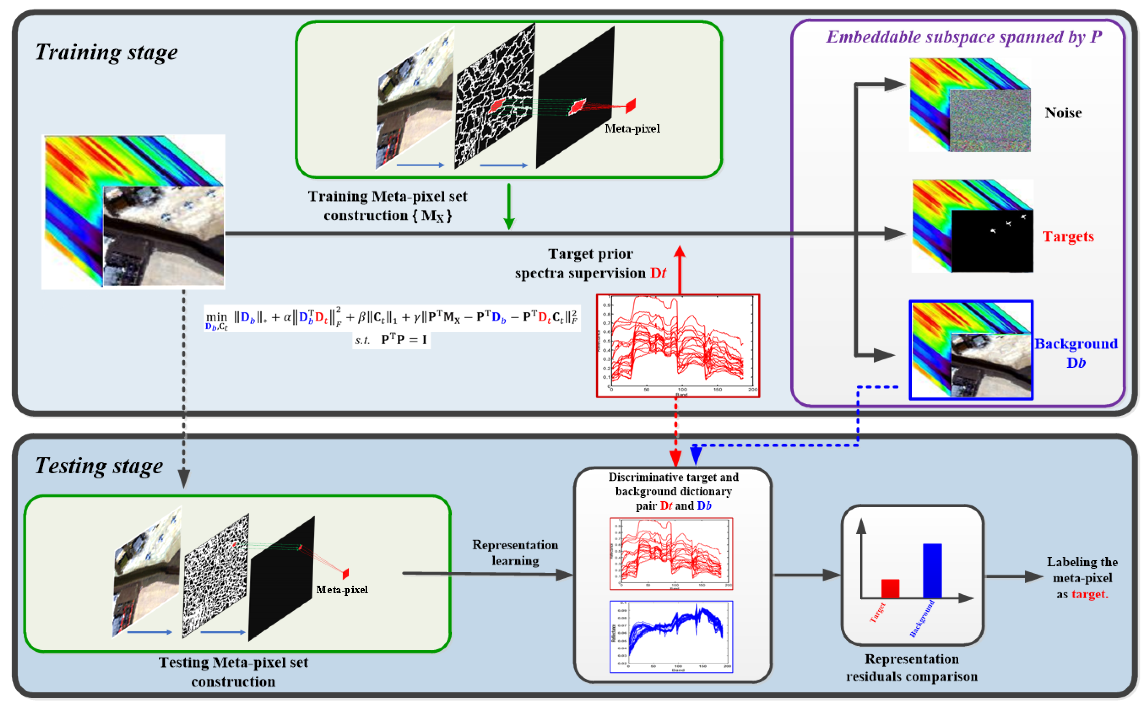
A Meta-pixel-driven Embeddable Discriminative background and target Dictionary Pair (MEDDP) learning model is established to efficiently learn a discriminative and compact background dictionary from the constructed meta-pixel set by introducing the discriminative structural incoherence. In addition, an adaptive low-dimensional embeddable subspace is jointly derived to reduce spectral redundancy and extract meaningful features, which can lead to more accurate characterizations of the target and background.
(3)
An efficient optimization algorithm is designed to solve the MEDDP model. The key variables, i.e., the background dictionary and orthogonal embeddable projection matrix are optimized iteratively to find the satisfied solutions. Furthermore, a novel meta-pixel-level target detection is performed based on the MEDDP model and some representation learning strategies. Experiments on several benchmark HSI datasets verify the effectiveness of the proposed method in comparison with several state-of-the-art HSI target detectors.
The remainder of this paper is structured as follows. Some key related works are introduced in Section 2. Section 3 presents the detailed descriptions for the proposed MEDDP model and the target detection strategy. Then, in Section 4, the experimental results and analysis are presented. Section 5 finally summarizes the full paper.

2. Related Works

Suppose an HSI dataset is with the size of h × w × B and contains several target object pixels of interest for detection given some prior target spectra. h and w respectively represent the height and width of the HSI scene. The data dimensionality, i.e., spectral band, is B . The observed 3-D HSI can be rearranged as a 2-D matrix by arranging the pixels in order. Thus, the HSI dataset is converted into the form of a matrix as X = [ x 1 , x 2 , , x N ] B × N with N = h × w . N is the total number of the HSI pixels, which is usually very large containing various land-cover objects, such as soil, gravel, vegetation, and buildings. Some important notations used in this paper are summarized in Table 1.

2.1. Low-Rank Modeling

Low-rank regularization, served as a metric to second-order (i.e., matrix) sparseness, has recently seen a surge of interest in theories, models, and applications. Robust principal component analysis (RPCA) is a representative low-rank modeling method to recover the low-rank component L from the corrupted noisy observations X by removing the sparse noise component E , which is mathematically formulated as below [25].
min   L , E r a n k ( L ) + λ E 0 s . t . X = L + E
where the parameter λ > 0 is used to balance the two terms in the objective function. In addition, the r a n k ( · ) function can be relaxed by nuclear norm · * , such that the problem can be readily solved by existing convex optimization tools. RPCA is essentially based on the hypothesis that data is drawn from a single low-rank subspace. However, high-dimensional optical data are generally distributed in a union of multiple low-dimensional subspaces. To better handle such complex structure of data, low-rank representation (LRR) has been suggested to pursue a low-rank representation matrix of a set of samples on a given dictionary D , which is formulated as follows [26,27].
min   D , E r a n k ( Z ) + λ E 0 s . t . X = D Z + E
It was obvious that an appropriately constructed dictionary D plays a key role in pursuing the desired optimal low-rank representation solution Z [28].

2.2. Sparse Representation Theory-Based HSI Target Detection

The sparse linear representation model based on an over-complete dictionary of primitives or signal atoms is a powerful tool to analyze the data with sparseness property [28,29,30,31]. A sufficiently sparse representation is informative for reasoning and decision-making. Therefore, the sparse representation theory has been introduced for HSI target detection. Sparse representation-based target detection (SRD) assumes that the pixels belonging to the same category are approximately located in a low-dimensional subspace, and employs the samples from both the target prior samples (dictionary) D t B × n t and the background samples (dictionary) D b B × n b to approximately reconstruct the label-unknown test pixel x as below.
x D t   c t + D b c b = D c
where D = [ D t , D b ] B × ( n t + n b ) is composed of the target and background samples, and c is the global representation vector of x , with D as the representation dictionary. The entities of c = [ c t , c b ] ( n t + n b ) reflect the contributions of the corresponding samples in representing x . Among the numerous potential solutions for model (3), if most of the entities of a solution are nearly equal to zero, the remaining non-zero entities will be very informative, and implicitly indicate the category of x , as target or background. Therefore, most of the entities of c are encouraged to be zero by introducing the following l0-norm based sparsity regularization.
min c c 0 s . t . x   D c
where the l0-norm · 0 counts the number of the nonzero elements of a vector. The solution can be obtained via some sparse optimization algorithms, e.g., orthogonal matching pursuit (OMP) [32]. However, the problem of searching for the sparest solution of an underdetermined linear equation is NP-hard [33]. Recent advances in the sparse representation and compressed sensing theories reveal that if the solution c is sufficiently sparse, one can use the following l1-minimization problem as a surrogate for the l0-minimization problem (4).
min c c 1 s . t . x   D c
The optimization problem (5) can be solved in polynomial time via some standard linear programming methods. As a result, solving (4) or (5) can lead to two sparse representation sub-vectors c t and c b corresponding to the target and background sub-dictionaries D t and D b . The recovery residuals ( x D b c ^ b ) and ( x D t c ^ t ) calculated based on the two sub-dictionaries are utilized for determining the label of test HSI pixel using the following thresholding operation.
Label ( x ) = Threshold ( x D b c ^ b 2 2 x D t c ^ t 2 2 )
Nevertheless, SRD does not consider the prior difference information between target and background. Different from SRD, SRBBH recovers the test pixels according to the two subspaces spanned by the background dictionary and the target-background combined dictionary based on the binary hypothesis test respectively, as shown below.
H 0 : x D b β ,   target   is   absent
H 1 : x D b γ b + D t γ t = D γ ,   target   is   present
The sparse representations of β and γ to (7) and (8) can be obtained by solving the following l0-norm minimization problems.
β ^ = min β x D b β 2 s . t . β 0 K 0
γ ^ = min γ x D γ 2 s . t . γ 0 K 1
where K 0 and K 1 mean the sparseness levels under the two hypotheses. Similar to (6), representation residuals derived from (9) and (10) are utilized for target detection.
Label ( x ) = Threshold ( x D b β ^ 2 2 x D γ ^ 2 2 )
The ideas of sparse and collaborative representations have proved to be efficient in SRD, SRBBH and their variants, such as the combined sparse and collaborative representation (CSCR) [21], the sparse and dense hybrid representation-based detector (SDRD) [22], and the binary class collaborative representation-based detector (BCRD) [20]. However, the performances of these methods are largely dependent on the high quality of the target prior samples and the background samples, which should be able to well characterize the complex statistical properties of the target and background. The target prior samples, as the known prior knowledge about the targets, are usually constructed from some standard spectral libraries or gathered in the field with handheld spectrometers. As for the construction of background dictionary, an adaptive scheme is commonly adopted based on a dual concentric window centered on the test pixel, with an inner window region (IWR) centered within an outer window region (OWR), such that the background dictionary can well characterize the local background statistics [18]. Unfortunately, there are no general rules for determining the appropriate IWR and OWR window sizes. In addition, the background dictionary constructed in this way failed to ensure the purity of the background because the inner window was a rectangle with a fixed size and might be contaminated by scattered targets.
Therefore, the problems of accurate and compact characterizations of the target and background dictionaries need further investigation. In addition, the intrinsic high-dimensionality, diversity, and heterogeneity properties of the HSI data will pose great challenges to the discriminative characterizations of the target and background, and harm the detection performance. As a result, we attempt to learn a global compact and discriminative target and background dictionary pair from the observed HSI by exploiting the advantages of superpixel segmentation, discriminative structural incoherence, and adaptive embeddable features learning, such that the spectra variability, mixture, high redundancy of HSI can be well dealt with for improved detection accuracy.

3. Metal-Pixel-Driven Embeddable Discriminative Target and Background Dictionary Pair Learning for HSI Target Detection

3.1. Meta-Pixel Set Construction

Superpixel segmentation can group spatial homogenous and perceptually uniform HSI regions and greatly reduce spectral variability and heterogeneity. And meanwhile, the computational efficiency can be improved by reducing redundancy between similar pixels [34]. As one of the most widely used algorithms for superpixel segmentation in HSI, entropy rate superpixel segmentation (ERS) is applied to the first three principal components after principal component analysis, and can efficiently get compact and homogeneous superpixels with similar sizes. Therefore, after segmenting the HSI data X = [ x 1 , x 2 , , x N ] B × N by ERS, a superpixel set of X , i.e., S X = { S c } , c = 1, 2…, C, containing C superpixels with N c pixels in the c-th superpixel can be obtained.
Although the pixels in each superpixel are spatial homogeneous and perceptually uniform, the spectral differences and variations between the pixels of superpixel still exist and will bring computational complexity. To smooth the spectral difference, one can intuitively find the center pixel of each superpixel by averaging all pixels as below.
δ c = 1 n c i n c x c i
where δ c is the center pixel of the c-th superpixel. x c i is the i-th pixel in the c-th superpixels. Nevertheless, the center pixel merges the pixels in the superpixel on average and fails to consider the superpixel local affinity manifold structure, which will be lost by the simple average operation.
To alleviate the issue, a novel meta-pixel is defined based on the superpixel by considering the manifold affinity relationship between each pixel with the center pixel. Thus, the informative prototype spectral signatures, i.e., the meta-pixel m c of the superpixel is calculated as below,
m c = i n c w c i x c i
where w c i reveals the manifold affinity of pixel x c i to the center pixel δ c of the c-th superpixel, which is inversely proportional to its distance to the center pixel of the superpixel and reflects the local manifold affinity property of the pixels within the superpixel.
w c i = e x p ( | x c i δ c | 2 k ) ,   c = 1 ,   2 ,   C ;   i = 1 ,   2 ,   n c
As shown in Figure 2, in comparison to the center pixel, the meta-pixel considers the weighted composition of the pixels in superpixel, such that the global and local manifold affinity structure can be simultaneously preserved to find the most typical spectral signatures. According to this, the meta-pixel set M X containing C training meta-pixels can be obtained.
M X = { m c } ,   c = 1 , 2 , , C
The constructed meta-pixel set can transform the target superpixel into a pure target or sub-pixel, inhibit the spectra heterogeneity and variability by efficiently clustering spatial and spectral similar pixels, and concurrently retaining the key spectral prototype signature and local manifold property of each superpixel.

3.2. MEDDP Model Formulation

In HSI target detection, the target pixel of interest only accounts for a small part of all the pixels in the whole HSI scene, and thus are sparse in quantity. On the other side, similar background pixels have similar spectral characteristics, and the types of background pixels are limited. Therefore, background pixels are correlative and usually fall into a low-dimensional subspace with the low-rankness property. As a result, the low-rankness prior can enable us to obtain a better estimation of the background from the training meta-pixel set. Therefore, the HSI meta-pixel dataset M X is modeled as a summative combination of a background dictionary D b B × n b with low-rankness, and the known target prior spectra D t B × n t regularized by a sparse target representation matrix C t , i.e., M X = D b + D t C t , resulting in the following model.
min D b , C t D b * + α Φ ( D b , D t ) + β C t 1 + γ M X D b D t C t F 2
where · * is the nuclear norm of matrix used to model and separate a low-rank background dictionary D b . The data reconstruction fidelity term M X D b D t C t F 2 is utilized to model the noise which is usually assumed identically and independently distributed Gaussian random variables. To alleviate the target prior spectrum scarcity problem, one can use some linear mixture model (LMM) and nonlinear mixture model (NLMM), to simulate and generate real-world target sub-pixel using pure prior target pixel and background pixel with varying fractions. The regularization term Φ ( D b , D t ) is expected to promote the discrimination between D b and D t . To achieve this aim, D b and D t should be as incoherent as possible. D t T D b calculates the coherence and correlation between D t and D b . Thus, minimizing D t T D b F 2 will lead to enhanced incoherence and discrimination between D t and D b , as formulated below,
min D b , C t , P D b * + α D t T D b F 2 + β C t 1 + γ M X D b D t C t F 2
Nevertheless, the original HSI data always contain hundreds of contiguous narrow bands and has high-dimensional redundant information. Based on the model (17), an orthogonal dimension reduction embeddable matrix P B × d   ( d < B ) with P T P = I is further incorporated and jointly learned to transform the learning of the background dictionary D b into a lower d-dimensional embeddable subspace. The complete formulation for our proposed meta-pixel-driven discriminative target and background dictionary pair model is as below,
min D b , C t , P D b * + α D t T D b F 2 + β C t 1 + γ P T M X P T D b P T D t C t F 2 s . t .   P T P = I
Compared to the primary model (17), the above model (18) can learn the background dictionary D b from the meta-pixel set M X in a jointly learned adaptive dimension-reduced embeddable subspace spanned by the projection matrix P , which can significantly reduce the spectral redundancy by extracting meaningful features.

3.3. MEDDP Model Optimization

For ease of optimization for model (18), two auxiliary variables J and L are first introduced to make the optimization problem separable and transform the formulation into the following equivalent one.
min D b , C t J * + α D b T D t F 2 + β L 1 + γ P T M X P T D b P T D t C t F 2   s . t . P T P = I ,   D b = J ,   C t = L
which can be solved based on the Inexact Augmented Lagrange Multiplier (ALM) scheme because of its efficiency [35]. Accordingly, the augmented Lagrangian function form of (19) is as follows.
( D b , C t , P , J , L , μ ) = J * + α D b T D t F 2 + β L 1 + γ P T M X P T D b P T D t C t F 2 + μ 2 D b J + Y 1 / μ F 2 + μ 2 C t L + Y 2 / μ F 2   s . t . P T P = I
where μ > 0 denotes the penalty parameter, while Y 1 and Y 2 denote the Lagrange multipliers. The optimization of problem (20) can be performed iteratively by updating D b , C t , P ,   J , L , and μ sequentially. The detailed steps are as follows
(1)
Update P by solving the following problem with the other variables fixed.
min P γ P T M X P T D b P T D t C t F 2   s . t . P T P = I
The optimization problem (19) can be converted into the following one.
min P   Tr ( P T ( M X D b D t C t ) ( M X D b D t C t ) T P )   s . t . P T P = I
Let R = ( M X D b D t C t ) ( M X D b D t C t ) T , and model (22) is further be rewritten in the form as below.
min P   Tr ( P T R P ) s . t . P T P = I
The solution can be got by solving the minimum eigenvalue problem as follows.
R P = λ P
The optimal solution is denoted as P * = [ p 1 ; p 2 ;   ·   ·   ·   ; p d ] , and the vector p i corresponds to the eigenvector of the i-th smallest eigenvalues.
(2)
Update J with the other variables fixed and solve the following problem.
min J 1 μ J * + 1 2 J ( D b + L / μ ) F 2
The optimal solution is obtained as J * = U 𝒮 1 / μ [ Σ ] V T with ( U , Σ , V ) = SVD ( D b + L / μ ) , and 𝒮 θ [ · ] is the soft thresholding shrinkage operator defined as below [15].
𝒮 θ [ 𝕩 ] = { 𝕩 θ ,     i f   𝕩 > θ   𝕩 + θ , i f   𝕩 < θ 0 ,         o t h e r w i s e
(3)
Update C t with the other variables fixed by solving the following problem.
min C t γ P T M X P T D b P T D t C t F 2 + μ 2 C t L + Y 2 / μ F 2
Calculate the derivative of the objective function in (27) w.r.t. C t and set it as zero obtaining the following equations.
2 γ D t T P P T ( D t C t M X + X b ) + μ ( C t L + Y 2 / μ ) = 0
The solution for C t is then got as follows.
C t = ( 2 γ D t T P P T D t + μ I ) 1 ( 2 γ D t T P P T M X 2 γ D t T P P T D b + μ ( L Y 2 / μ ) )
(4)
Update D b with the other variables fixed by solving the following problem.
min D b α D t T D b F 2 + γ P T M X P T D b P T D t C t F 2 + μ 2 D b J + Y 1 / μ F 2
Calculate the derivative of the objective function in (30) with respect to D b and set it as zero. The solution for D b can be got via the equations in (31) and (32).
2 D t D t T D b + 2 γ P P T ( D b ( M X D t C t ) ) + μ ( D b ( J Y 1 / μ ) ) = 0
D b = ( ( 2 α I + 2 γ P P T + μ I ) ) 1 ( 2 γ ( M X D t C t ) + μ ( J Y 1 / μ ) )
(5)
Update L with the other variables fixed by solving the following problem.
min L β μ L 1 + 1 2 L ( C t + Y 2 / μ ) F 2
Let Q = C t + Y 2 / μ , the optimal solution to (33) is obtained using the thresholding shrinkage operator as in (26).
(6)
Update the Lagrange multipliers and penalty parameter:
{ Y 1 = Y 1 + μ ( D b J ) Y 2 = Y 2 + μ ( C t L ) μ = m i n ( ρ μ , μ m a x )
As summarized in Algorithm 1, the optimization processes from (1) to (6) are alternatively and iteratively performed until the convergence conditions are reached. The major computational loads of Algorithm 1 lie in solving (25), (27), and (30) because they involve singular value decomposition (SVD) and matrix inversion. SVD in (25) is operated for B × n b matrix and the computational complexity is 𝒪 ( B 3 ) . Matrix inversion and multiplication in solving (27) cost 𝒪 ( n t 3 + n t B d + n t 2 d ) . Also, matrix inversion for solving (30) costs 𝒪 ( B 3 ) since B d . The main computational complexity of Algorithm 1 is 𝒪 ( τ ( B 3 + n t 3 + n t B d + n t 2 d ) ) , with τ as the iteration number.
Algorithm 1. Solving problem (18) using Inexact ALM.
Input: Meta-pixel set M X , target prior spectra D t ,   μ m a x = 10 8 ,   ρ = 1.1 ,   ϵ = 10 6 ,   μ = 10 5 ,   α ,   β ,   and   γ . Reduced dimension d.
Initialization: Initialize P by PCA, D b = C t = Y 1 = Y 2 = 0 .
Whilenot convergencedo
1. Update P ,   J ,   C t ,   D b ,   L by successively solving the sub-problems in (23), (25), (27), (30) and (33).
2. Update the Lagrange multipliers and penalty parameter as in (19).
3. Examine the convergence conditions: D b J F 2 / M X F 2 < ϵ   and   C t L F 2 / M X F 2 < ϵ
End while
Output: D b   and   P .

3.4. Meta-Pixel-Level Target Detection Based on MEDDP Model

With the optimal target and background dictionary pair derived from the MEDDP model in a lower-dimensional embeddable subspace, superpixel segmentation is performed in testing to find perceptually uniform regions of HSI as in the training stage, and then obtain the testing meta-pixel set containing V meta-pixels according to (11)–(15).
Subsequently, a novel meta-pixel-level target detection is designed instead of the traditional pixel-level target detection. Specifically, each testing meta-pixel m v , v = 1 , 2 , , V is respectively represented by the target and background dictionaries D b and D t as in SRD and BCRD, or the combination of them as in SRBBH. The label of the testing meta-pixel m v is then determined by checking the difference between the representation residuals of m v over the target and background dictionaries, or their combination. Namely, the labeling of testing meta-pixel is determined by checking the corresponding representation residuals. This paper will combine the proposed MEDDP model with three state-of-the-art representation strategies, including SRD, SRBBH, and BCRD, for performance evaluations in the experimental part. Take SRBBH for example, the sparse representations of β and γ of m v regarding the background dictionary D b and target-background combined dictionary D = [ D b , D t ] can be obtained by solving the following l0-norm minimization problems.
β ^ = min β m v D b β 2 s . t . β 0 K 0
γ ^ = min γ m v D γ 2 s . t . γ 0 K 1
where K 0 and K 1 mean the sparseness levels. The representation residuals derived from (35) and (36) are then utilized for target detection.
Label ( m v ) = Threshold ( m v D b β ^ 2 2 m v D γ ^ 2 2 )
If the residual is bigger than a certain threshold, the meta-pixel will be labeled as background otherwise it will be labeled as a target. The complete procedures for target detection are shown in Algorithm 2.
Algorithm 2. MEDDP and meta-pixel-based target detection.
Input: HSI dataset X , target prior spectra D t , tradeoff parameters ,   α ,   β ,   and   γ . Reduced dimension d.
1. Construct a training meta-pixel set of X based on ERS and local manifold preservation.
2. Obtain the optimal target and background dictionary pair by solving Algorithm 1.
3. Construct testing meta-pixel set, and use the obtained dictionary pair for me-ta-pixel-level target detection via different representation-based target detection strat-egies, such as the SRBBH presented in (35)–(37).
Output: Detection map

4. Experimental Verifications

Numerous experiments will be performed in this part to test the performance of the proposed MEDDP model and the meta-pixel-based target detection method in comparison with several representative and state-of-the-art detectors on benchmark HSI target detection datasets.

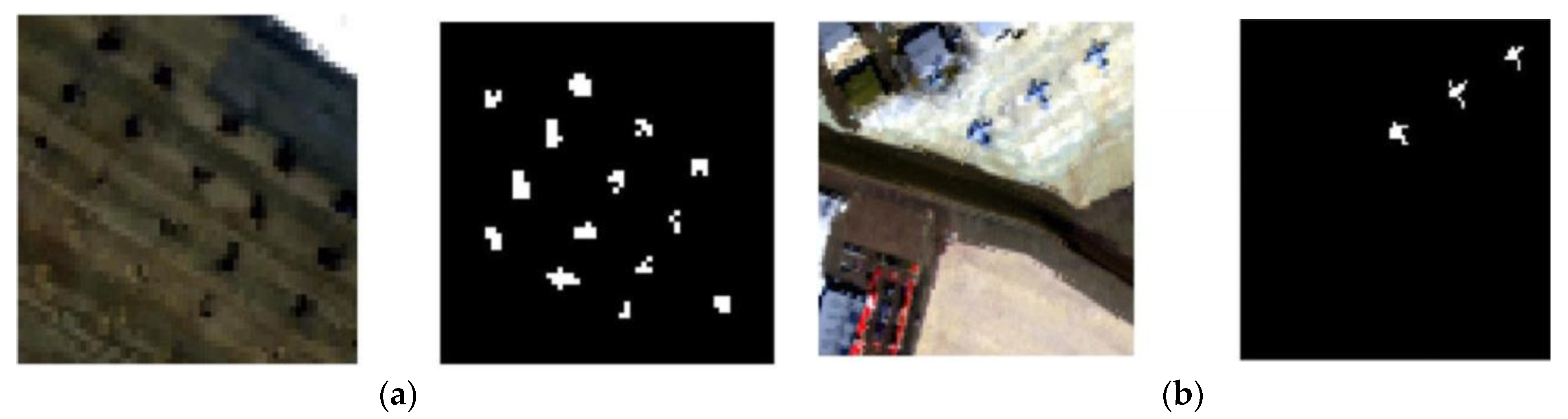
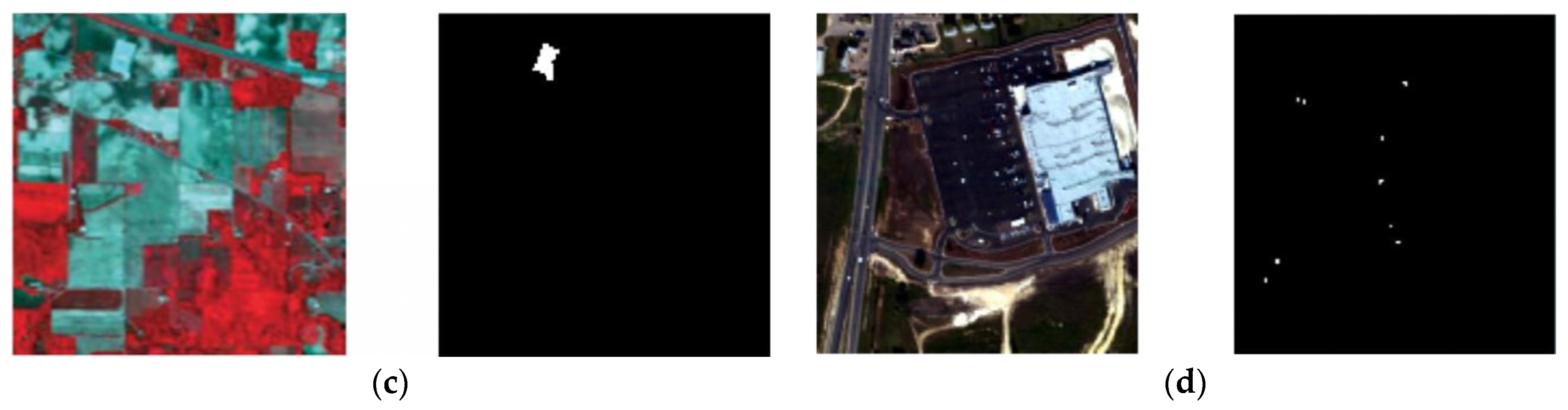
4.1. Benchmark HSI Datasets

Some benchmark HSI target detection datasets, i.e., the AVIRIS, HYDICE, and Indian Pines datasets with both relatively scattered and aggregated targets, were adopted in the experiments for performance evaluations of different methods.
More specifically, the AVIRIS dataset was collected by the Airborne Visible/Infrared Imaging Spectrometer (AVIRIS) in San Diego with a spatial resolution of 3.5 m. The dataset retains 189 spectral bands by discarding the low signal-to-noise, water absorption, and bad bands (1–6, 33–35, 97, 107–113, 153–166, and 221–224) [36]. Two sub-datasets, including AVIRIS I, AVIRIS II, and their corresponding ground-truth information for the target of interests are shown in Figure 3a,b, the spatial size of which are 60 × 60 pixels and 100 × 100 pixels, respectively. As illustrated in Figure 3c, the Indian Pines dataset is a scene of Northwest Indiana collected by an AVIRIS sensor [5]. The spatial size of the scene is 145 × 145 pixels with 220 spectral bands covering the wavelength range from 375 nm to 2500 nm. Multiple bands with noise and water absorption, i.e., 104–108, 150–163, and 220, were removed, leaving a total of 200 spectral bands used in the experiments [11,12]. The stone and steel tower with 93 pixels is selected as the targets to be detected.
The third data set was collected by the HYDICE sensor with a spatial resolution of 2 m and 210 spectral bands [20]. After removing the low signal-to-noise ratio, water absorption, and bad bands, including the 1–4, 76, 87, 101–111, 136–153, and 198–210 bands, 162 bands remained. The HYDICE data set and its ground-truth information are shown in Figure 3d, which has 150 × 150 pixels, and the vehicles with the size of 21 pixels were selected as the targets for detection.

4.2. Comparison Methods and Performance Evaluation Metrics

Our HSI target detection approach is compared with several frequently referred state-of-the-art approaches, including three classical methods (i.e., ACE, CEM, and SMF), three sparse and collaborative representation-based detectors (i.e., SRD, SRBBH, and BCRD), and the dictionary learning based detector (i.e., SLRMDD). A detailed description of these methods is enumerated as follows.
(1)
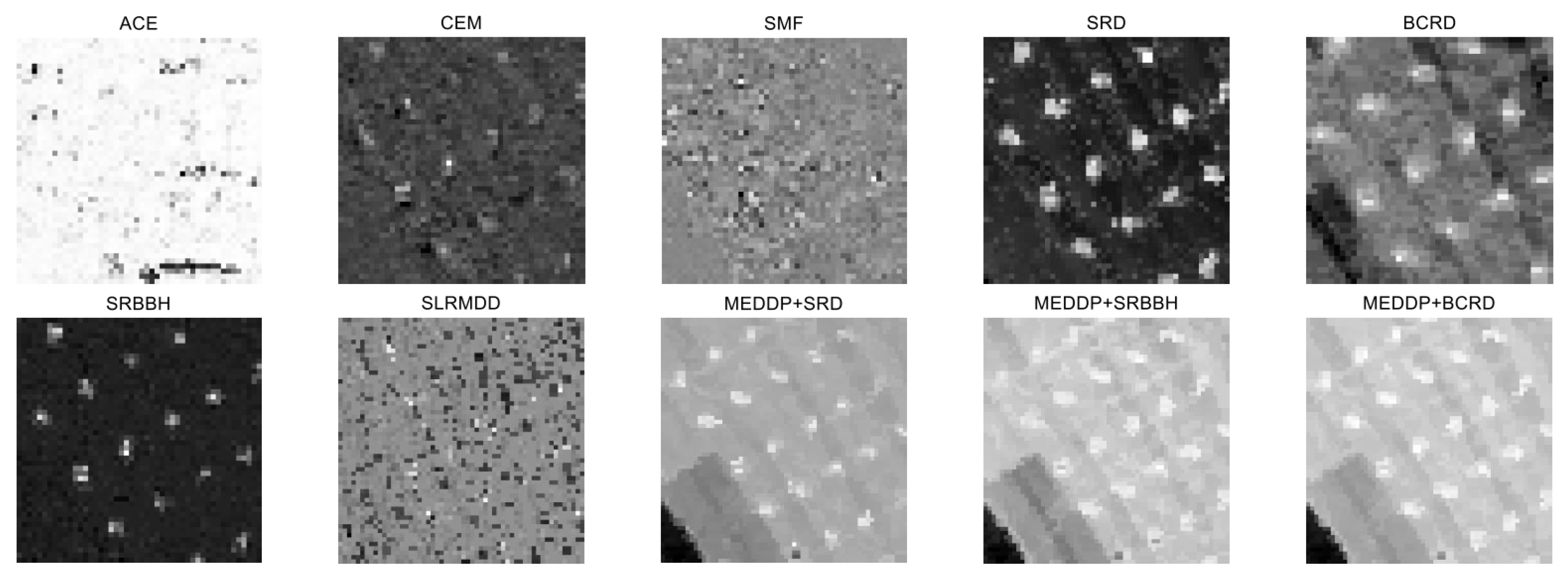
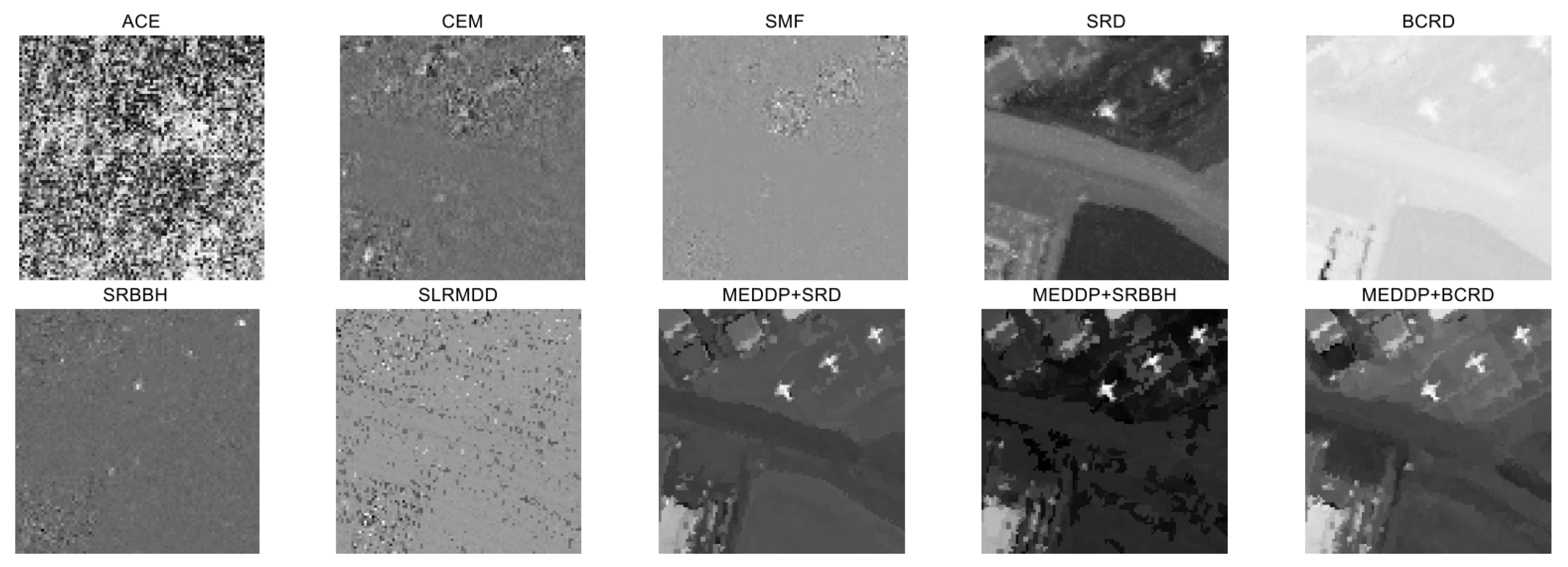
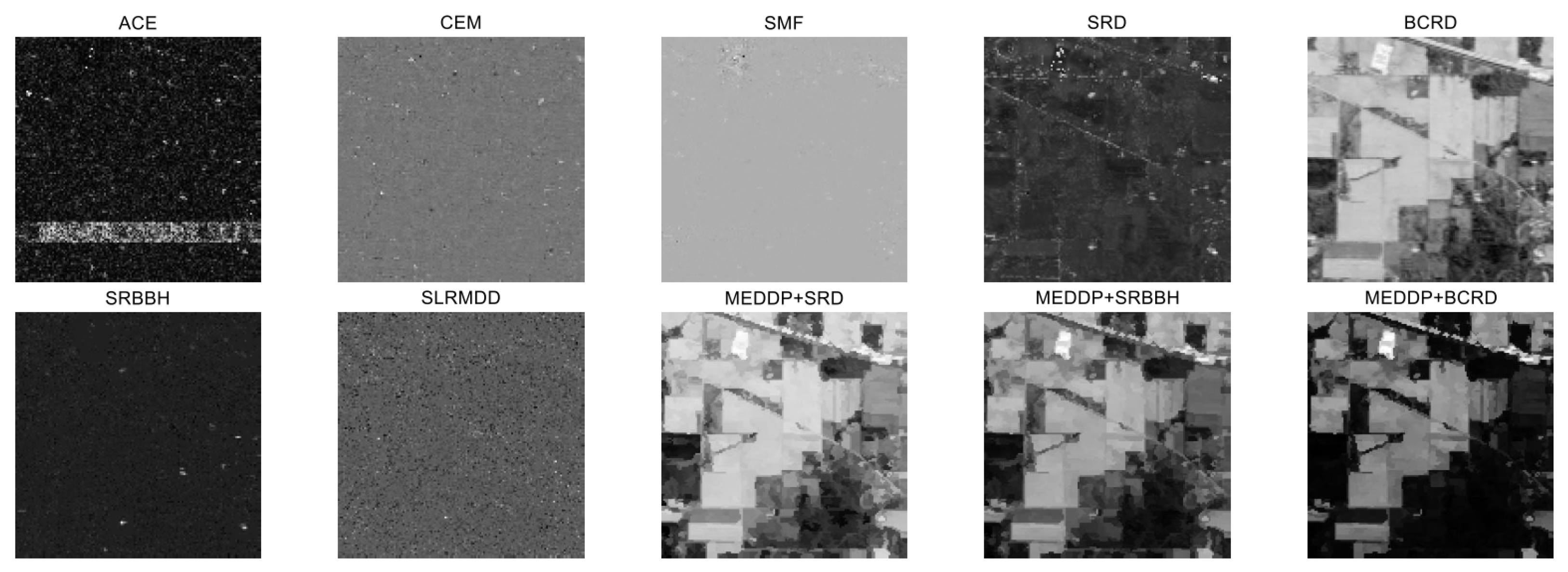
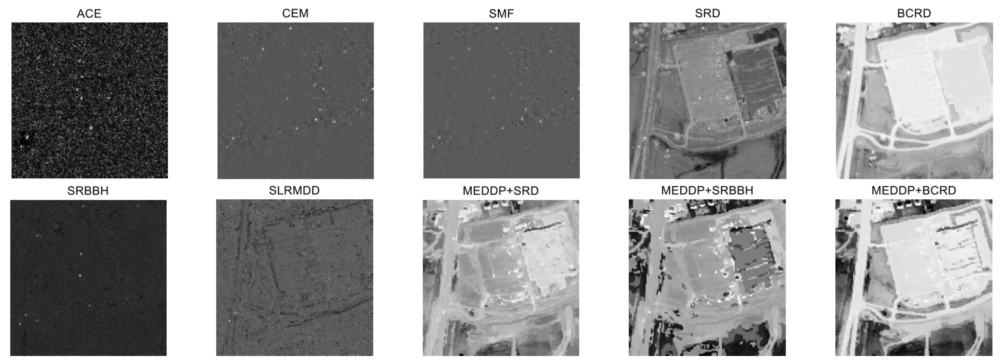
ACE: ACE is a background unstructured detector by assuming that the background has the same covariance structure but different variances under the two hypotheses [9].
(2)
CEM: CEM detects target by designing a finite impulse response filter (FIRF) using the known target spectrum and minimizing the energy of the interference signal. However, CEM fails to consider the assumption of data distribution, which will restrict its performance [37].
(3)
SMF: Different from CEM, the SMF detector estimates the background covariance matrix and then employs the generalized likelihood ratio test for detection with only a single target spectrum, which cannot fully model the diversity of target spectra [10].
(4)
SRD: SRD represents a test pixel using the target and background combined dictionary, and then determines the label of test pixel (background or target) by examining which sub-dictionary yields a smaller representation residual for the test pixel [18].
(5)
SRBBH: SRBBH combines the idea of binary hypothesis and sparse representation, in which the test pixel is respectively represented by the background dictionary, and the background and target combined dictionary under the two hypotheses that the target is present or absent. The derived representation errors under the two hypotheses are used for the final detection decision [19].
(6)
BCRD: In BCRD, both pixels in the background and pixels in the target can be collaboratively represented by some pixels of the image. The detection result is achieved by estimating the residual difference of two collaborative representations [20].
(7)
SLRMDD: SLRMDD is based on sparse and low-rank matrix decomposition and regards the given HSI as a composition of the sum of low-rank background HSI and a sparse target HSI containing targets via a target dictionary constructed from some online spectral libraries. Strategy one is used for target detection by combining the separated background dictionary with the SRBBH detector. The ratio between the two key parameters is set as 5/2 [4].
As previously mentioned, as a fundamental dictionary construction method, our MEDDP model is applied with the state-of-the-art SRD, SRBBH, and BCRD for detection, which can clearly show the advantages of the proposed dictionary construction and the meta-pixel-level target detection strategies. For the AVIRIS dataset, the sizes of the outer-window and inner-window used to construct the local background dictionary were empirically set as 17 × 17 and 7 × 7 for the above comparing method. For the Indian Pines and HYDICE datasets, the sizes for the dual windows in the comparative methods are 13 × 13 and 5 × 5. The receiver operating characteristic (ROC) curve was used to depict the relationship between the probability of detection and false alarm rate. The detector with a higher detection rate under the same false alarm rate level or the detector with the same detection rate with a lower false alarm rate level is claimed to have better detection performance. Despite the ROC curve, the area under the curve (AUC) was also used as a quantitative indicator for performance evaluation [38]. A detector with a larger AUC value means better detection performance.

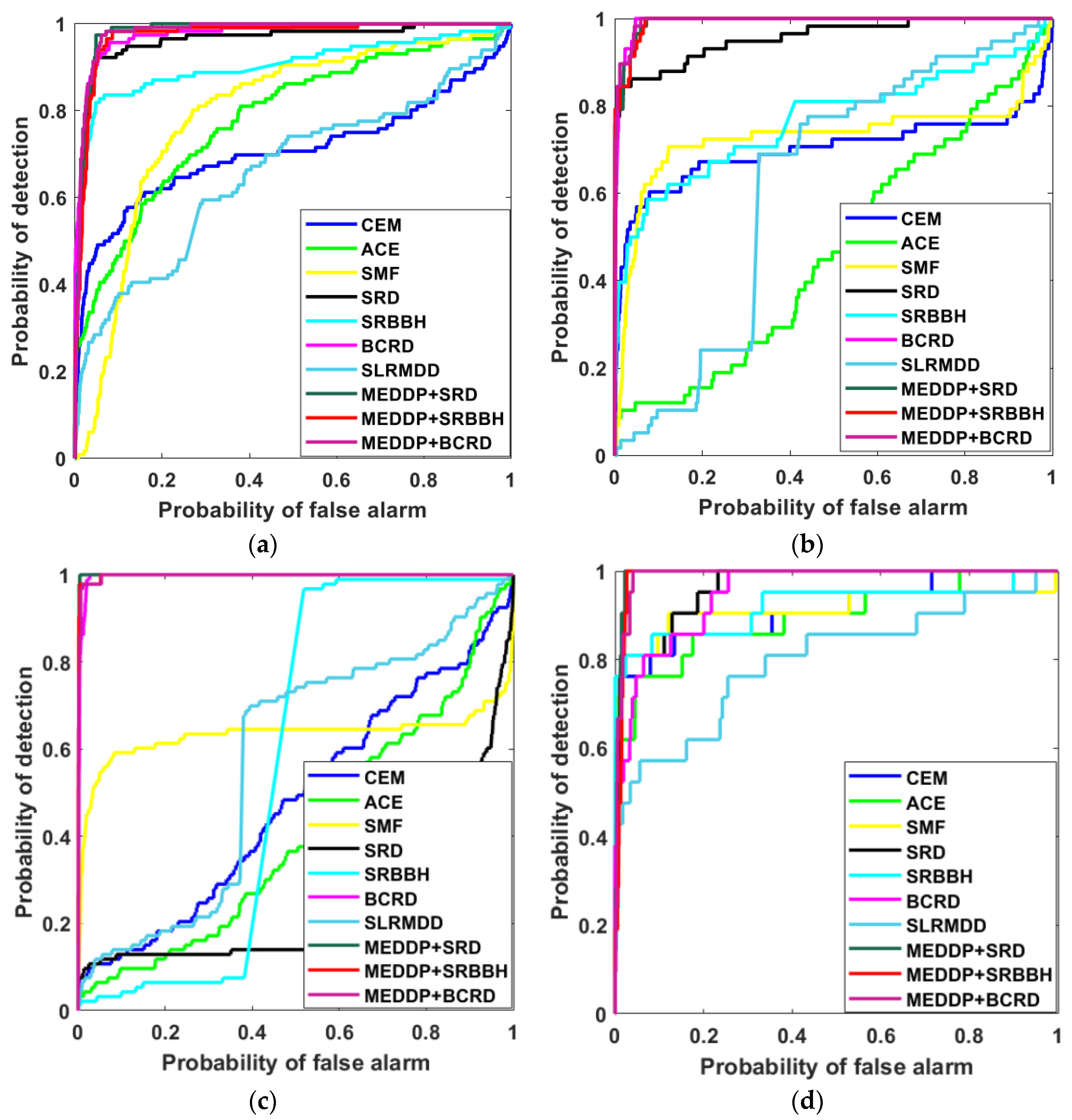
4.3. Qualitative and Quantitative Results

The detection maps for the comparative methods on different datasets are shown in Figure 4, Figure 5, Figure 6 and Figure 7. Intuitively, a good detector should have a higher true detection rate and lower false alarm rate by strengthening the differences between the target and background. In comparison with the ground truth maps of different datasets, the detection maps obtained by the classic ACE, CEM, and SMF detectors cannot clearly illustrate the location of the targets, and the target and background differences are not well enhanced by these detectors. Take the AVIRIS I and AVIRIS II datasets, for example, the detection maps of ACE are rambling with low detection accuracy. And the CEM and SMF can only roughly indicate the approximate locations of the targets, which might lead to extensive false alarms. Compared with SRD, SRBBH, BCRD, and SLRMDD, the target locations in the detection maps of the proposed MEDDP method in combination with SRD, SRBBH, and BCRD, are visually more apparent, which means that the proposed methods have better abilities in background suppression and target enhancement.
The target edge area and shape can be well highlighted, especially for the AVIRIS II and Indian Pines datasets, where the differences between target and background can be observed. In addition to visual observation of the qualitative detection maps for performance evaluations of different methods, the ROC curves of all the comparing methods are shown in Figure 8, and the AUC values were further used as a quantitative metric for more accurate evaluations, and the detailed results were reported in Table 2. The best results are shown in bold with the second-best underlined. Based on the comprehensive analyses of qualitative and quantitative results, one can see that the proposed MEDDP model can generally yield very promising performance when combing with different representation learning-based detectors, i.e., MEDDP + SRD, MEDDP + SRBBH, and MEDDP + BCRD. Especially when comparing with the basic detectors SRD, SRBBH, and BCRD, the improvements are significant, which can verify the benefits of the MEDDP model in precisely characterizing the discrimination between the target and background and keep a good balance between suppressing background and highlighting target.

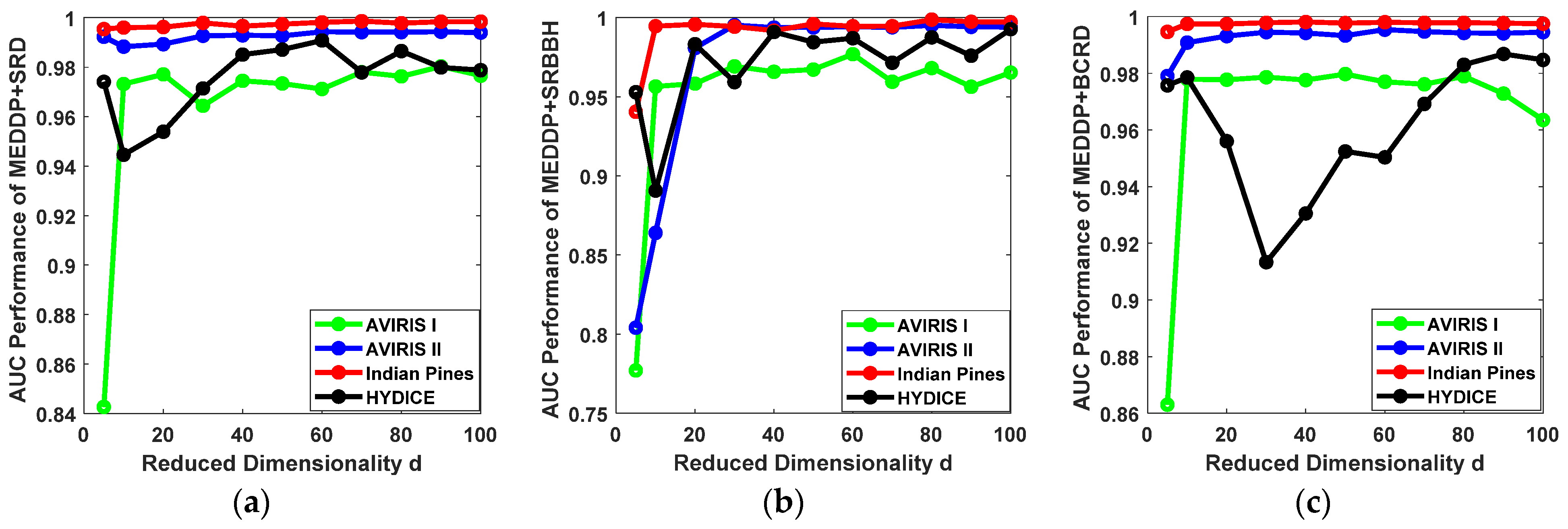
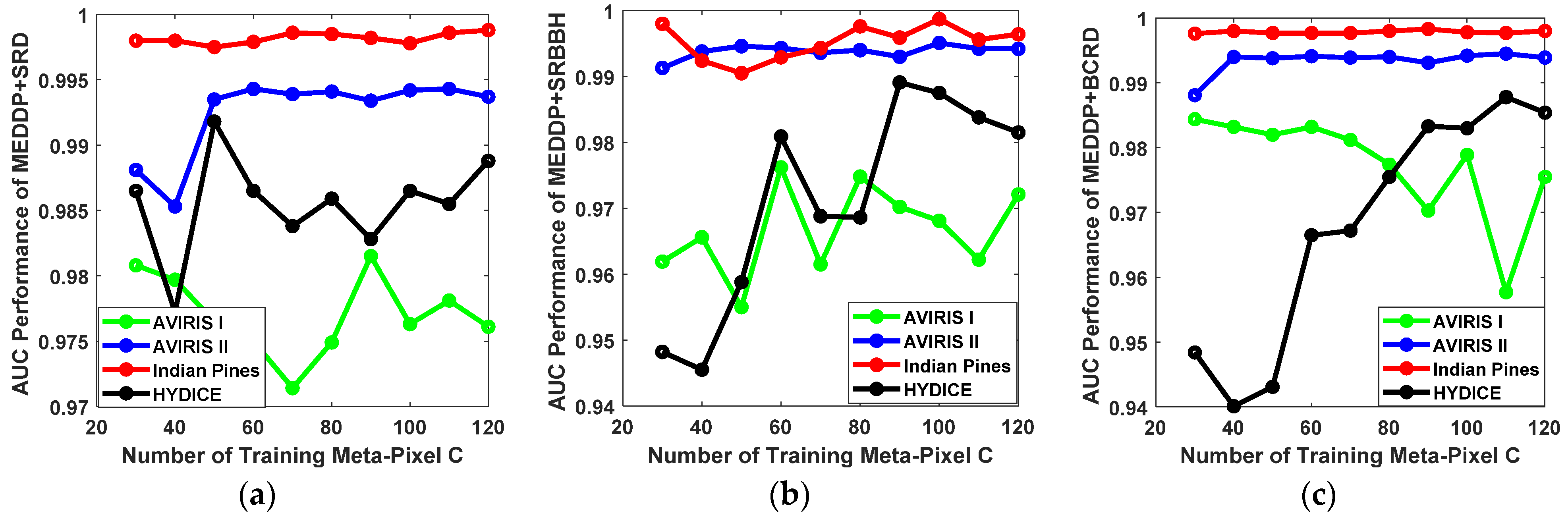
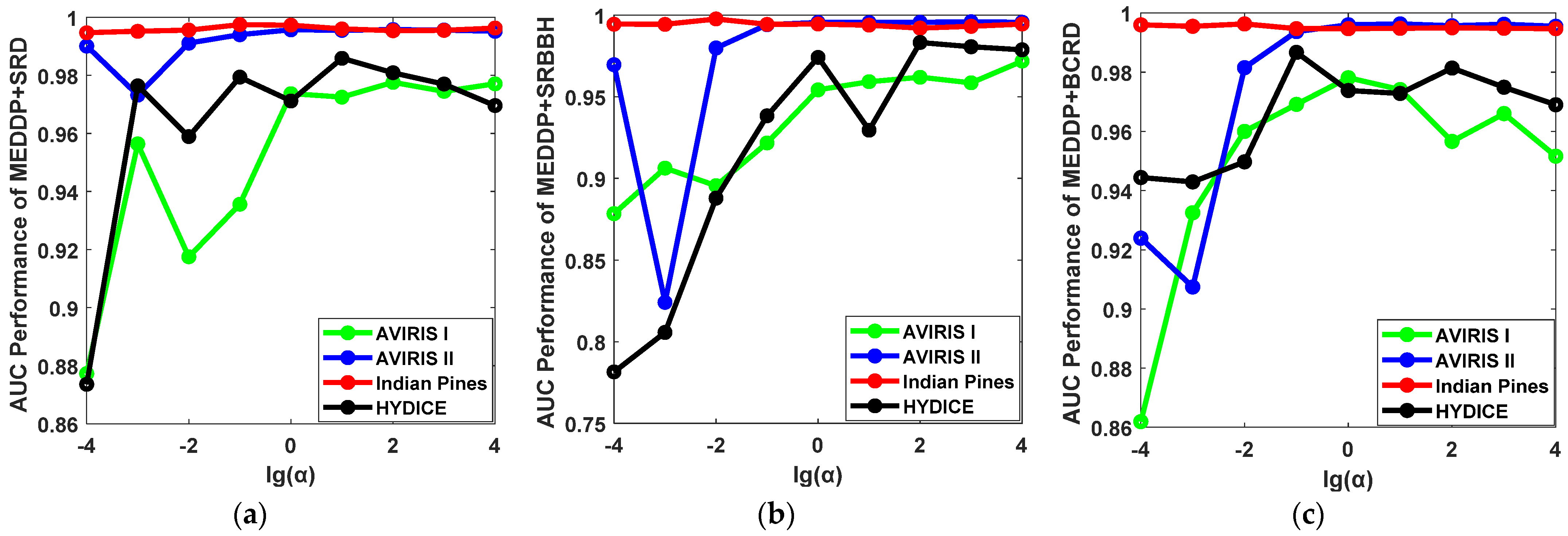
4.4. Parameters Analysis and Convergence Analysis

The performance of the proposed detection method is affected by the several key parameters, which are needed to be properly set, including the balancing parameters α, β, and γ in the model (18), the reduced dimensionality d, the dictionary atoms for the background (number of the training meta-pixels) C in MEDDP model, and the number for the testing meta-pixel V in the meta-pixel-level target detection. This section will study the proper settings of these parameters in a relatively small parameter range.
(1)
Influence of the Reduced Dimensionality d.
By considering the original dimensionality of the HSI data, the reduced dimensionality d is empirically selected from the candidate set {5, 10, 20, 30, 40, 50, 60, 70, 80, 90, 100}. The AUC performance variations of MEDDP + SRD, MEDDP + SRBBH, and MEDDP + BCRD, w.r.t different reduced dimensionality on the four HSI datasets are illustrated in Figure 9. From the figures, one can see that a relatively high dimensionality can generally lead to better detection performance on the AVIRIS I and Indian Pines data sets. However, a too high dimension d might introduce redundancy and limit the discrimination between the target and background dictionaries. And meanwhile, the risk of over-fitting and computational complexity will increase, which will yield fluctuating or even reduced performance. The detection performances for MEDDP + SRD, MEDDP + SRBBH, and MEDDP + BCRD on the AVIRIS II and Indian Pines data sets show better robustness to the variations of the reduced dimensionality d. Take the Indian Pines data set, for example, a comparative performance can be achieved when d = 10. Through comprehensive consideration of all the results on different data sets and different methods, the optimally reduced dimensionality d can be empirically set and tuned around 90, by which a promising detection performance can be expected to be achieved by the proposed MEDDP + SRD, MEDDP + SRBBH, and MEDDP + BCRD.
(2)
Influence of Number of Training Meta-Pixel C.
One of the key steps in the proposed MEDDP model is the training meta-pixel set construction, which is used to alleviate the spectral variability and heterogeneity and find the typical spectral signatures of HSI to enable the following discriminative target and background dictionary pair learning. The selection of the number of training meta-pixel C will also determine the number of the background dictionary atoms and is critical to the quality of the dictionary pair, which will affect the final target detection performance. The candidate number of training meta-pixel C for is empirically selected from the set {30, 40, 50, 60, 70, 80, 90, 100, 110, 120}. The ROC performance variations of our proposed detectors with different numbers of training meta-pixel C on different data sets are shown in Figure 10 From the subplots, one can see that the detection performance on the AVIRIS II and Indian Pines are more robust to the variations of C. While for the AVIRIS I and HYDICE data sets, the detection performances more susceptible to different settings of C. More training meta-pixel tends to yield better detection performance. However, the computational complexity will also increase with more training meta-pixels. A balance should be kept between performance and consumption. Based on the results and analyses, the number of training meta-pixel C can be set around 100.
(3)
Impact of the Number of Testing Meta-Pixel V.
In the testing stage, a novel meta-pixel-level target detection strategy instead of pixel-level target detection has been devised. Similar to the training phase, the HSI dataset is firstly segmented into a certain number of superpixels to construct the testing meta-pixel set. In comparison to the number of the training meta-pixel, the number V for the testing meta-pixel should be larger, which can ensure a finer segmentation and detection. The candidate number V for testing meta-pixel is selected from the set {300, 600, 900, 1200, 1500, 1800, 2100, 2400, 2700, 3000}. The ROC performance variations for our proposed detectors with different numbers of testing meta-pixel V on different data sets are shown in Figure 11. With larger testing meta-pixel numbers, promising detection performances can be consistently achieved on the AVIRIS I, AVIRIS II, and Indian Pines data sets. While for the HYDICE data set, the detection performance improves with the increase of the number of testing meta-pixel. As a result, the number of testing meta-pixel V is suggested to be set around 2000 in practice.
(4)
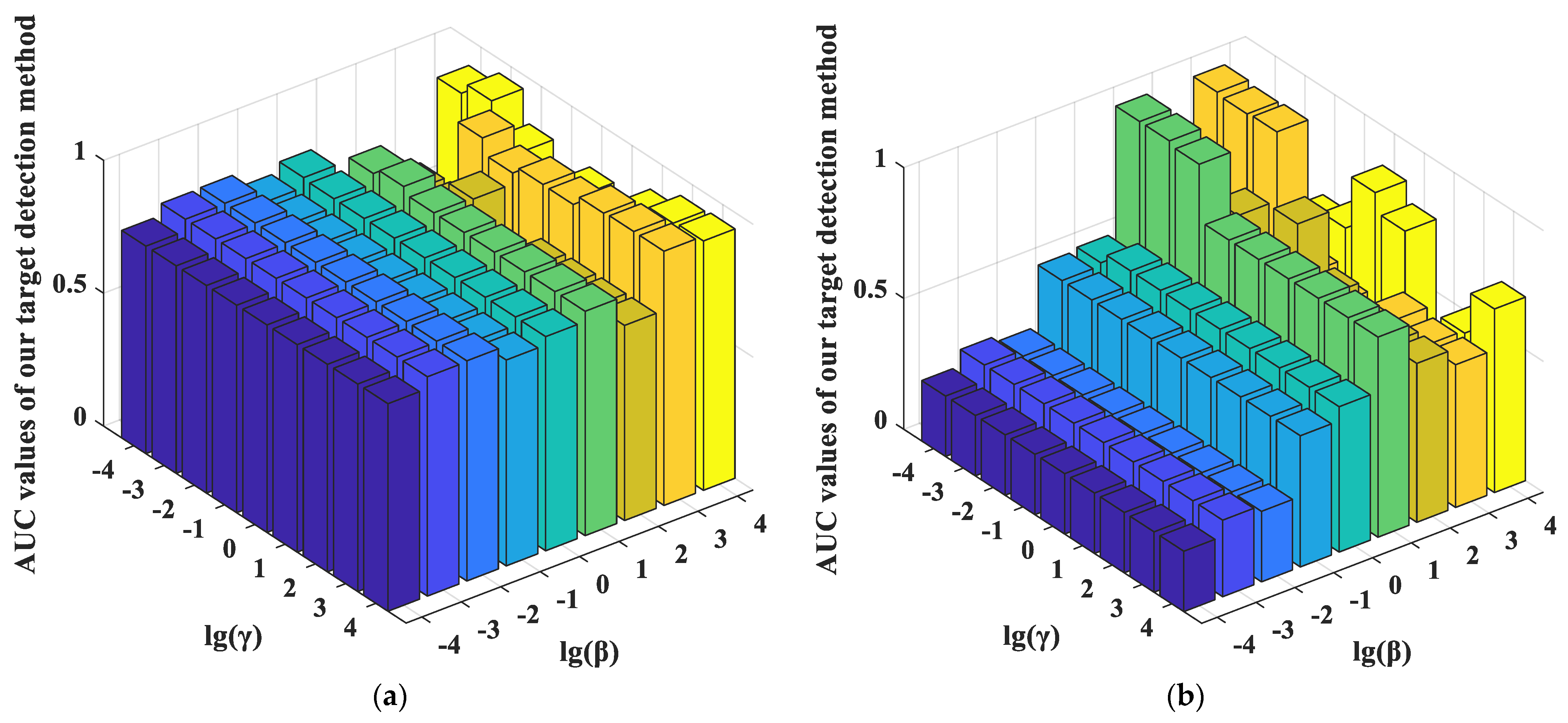
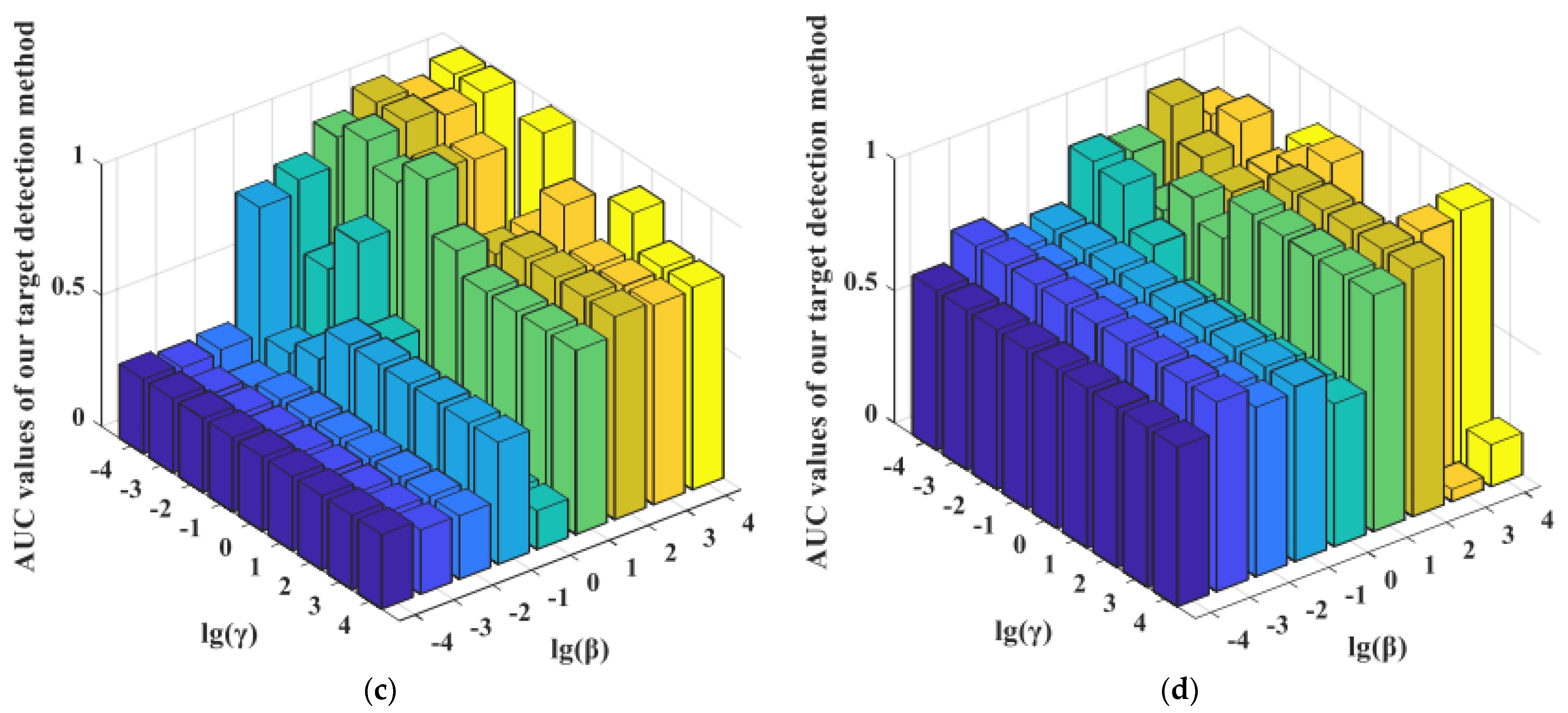
Influence of the Balancing Parameters α, β, and γ.
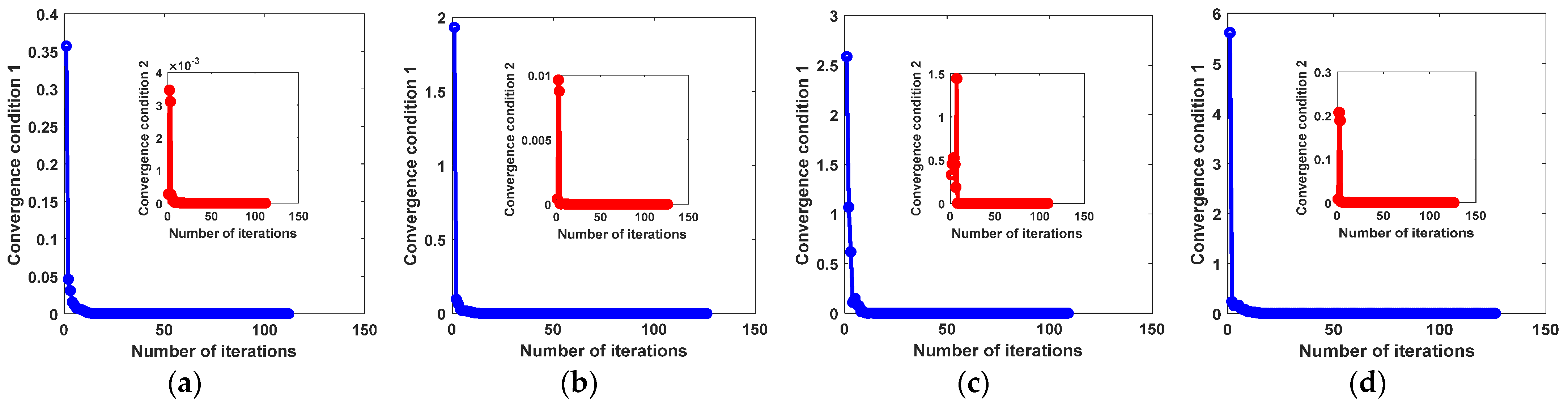
For the balancing parameters α, β, and γ in the MEDDP model (16), α is fixed when adjusting β and γ within the candidate parameter set {10−4, 10−3, 10−2, 10−1, 100, 101, 102, 103, 104}. The performance variation of the detector regarding the log-scaled β and γ were reported in Figure 12. From the MEDDP model formulation, one can see that a larger α will help enhance the discrimination between the target and background dictionaries by minimizing their correction, which can be observed from the experimental curves in Figure 12. However, an extreme large might lead to over-fitting, thus the optimal α can be selected from [10−1, 102]. In addition, the ROC performance variations for our proposed detectors w.r.t different settings of the balance parameters β and γ with the optimal α fixed on different data sets are shown in Figure 13. The detection performances show higher sensitivity to the settings of β and γ. By comprehensively analyzing the performance variations rule w.r.t the different combinations of β and γ, the suggested setting ranges for the two parameters are β ∈ [101, 104], γ ∈ [10−1, 102]. There is a higher probability that stable and satisfying performance can be yielded with these suggested parameters.
(5)
Convergence Analysis of the Optimization Algorithm
For solving the proposed MEDDP model, an inexact ALM-based optimization algorithm has been devised and presented in Algorithm 1. The convergence property of the algorithm is dependent on the proper settings of the balancing parameters α, β, and γ, and will finally affect the performance of the model. Two key convergence conditions, i.e., D b J F 2 / M X F 2 < ϵ and C t L F 2 / M X F 2 < ϵ , were used as the judging criteria to indicate the convergence performance of the optimization algorithm, the convergence curves on different data sets of which were shown in Figure 14. It can be seen from the curves that the optimization algorithm converges well in practice, and the convergence conditions can be quickly reached within the appropriate 20 iterations. As a result, the convergence curves, as well as the detection performance reported in the experimental results, can verify the effectiveness of the optimization algorithm.
Among the comparative methods, as shown by the experimental results, the classic methods, such as the ACE, CEM, and SMF, are always dependent on some specific prior assumptions, which are not true due to the high dimensionality and complexity of the HSI spectra, which will limit the generalization ability in more application scenarios. In contrast, such assumptions are not needed in some state-of-the-art representation learning-based HSI target detectors, including the SRD, SRBBH, and BCRD, which are developed on the theory of linear subspace, and show more flexibility in modeling the HSI spectral variations. However, SRD and SRBBH cannot achieve promising performance without accurate target and background dictionaries, especially in the case of aggregated larger targets.
The above classical target detection techniques, such as the SRD, SRBBH, and BCRD, adopt the local adaptive scheme-based sliding dual-window for background dictionary construction. The sizes for the IWR and OWR are hard to be set. As a result, the purification and compactness of the obtained background dictionary cannot be guaranteed. By contrast, the proposed MEDDP model is tailored to alleviate the problems of spectral high-dimensionality, variability, and heterogeneity, and improve the discriminative characteristics between the target and background dictionaries. In addition, the experimental results show that the proposed method can consistently yield superior performance. The reasons can be stated as follows. Firstly, the newly developed meta-pixel set construction method can efficiently alleviate the problems of spectral variability and heterogeneity by discovering the typical spectral signatures. Meanwhile, by reducing the spatial redundancy between similar pixels via meta-pixel construction, the computational efficiency can be also improved. Secondly, a discriminative target and background dictionary pair was obtained by low-rank matrix decomposition, structural incoherence based on the advantages of the meta-pixel. In addition, the joint learning strategy of the dictionary pair and adaptive subspace can enhance the intra-class similarity and inter-class dissimilarities by reducing spectral redundancy.
Even though the proposed method can estimate a discriminative target and background dictionary pair to enlarge the response differences between the target and background pixels, the background suppression problem is not considered in the proposed method. A perfect target detector should simultaneously highlight the target and suppress the background. Another key problem is the transferability of the detector. This is because the target prior spectra are usually acquired from some standard spectral libraries collected with handheld spectrometers. However, the targets to be detected are always remotely sensed in the wild. A distribution bias will inevitably exist between them. Thus, the problems of background suppression and transferability of the method need to be solved in future.

5. Conclusions

This paper has developed a sparse and low-rank modeling-based MEDDP method to learn a meta-pixel-driven discriminative target and background dictionary pair for meta-pixel-level target detection. Specifically, the meta-pixel set is constructed by taking the advantages of superpixel segmentation and the local manifold structures to find the most informative and typical prototype spectral signatures of HSI. Afterward, the meta-pixel driven embeddable discriminative target and background dictionaries learning model is established by incorporating the prior target spectrum information, structurally incoherent constraint, and the low dimensional subspace learning, to simultaneously enlarge the dissimilarity between the target and background dictionaries and find the meaningful low-dimensional features with spectral redundancy reduced. Therefore, the obtained discriminative and compact target and background pair can finally boost the meta-pixel-level target detection performance, as verified by the experimental results on benchmark HSI datasets through comparisons with different representative detection methods.

Author Contributions

All the authors made significant contributions to the study. T.G. and F.L. conceived and designed the global structure and methodology of the manuscript. L.F. and B.Z. provided some valuable advice and proofread the manuscript. All authors have read and agreed to the published version of the manuscript.

Funding

This work was supported in part by the National Natural Science Foundation of China under Grant 62071340 and 61801336, in part by the Natural Science Foundation of Chongqing under Grant cstc2020jcyj-msxmX0636, in part by the Key Scientific and Technological Innovation Project for “Chengdu-Chongqing Double City Economic Circle” under Grant KJCXZD2020025, in part by the Science and Technology Development Fund, Macau SAR under Grant 0073/2019/A2, in part by the Macao Young Scholars Program under Grant AM2020008, and part by the 2019 Outstanding Chinese and Foreign Youth Exchange Program of China Association of Science and Technology (CAST).

Institutional Review Board Statement

Not applicable.

Informed Consent Statement

Not applicable.

Data Availability Statement

The data presented in this study are available upon request from the author.

Conflicts of Interest

The authors declare no conflict of interest.

References

  1. Wang, Y.; Wang, L.; Yu, C.; Zhao, E.; Song, M.; Wen, C.-H.; Chang, C.-I. Constrained-target band selection for multiple-target detection. IEEE Trans. Geosci. Remote Sens. 2019, 57, 6079–6103. [Google Scholar] [CrossRef]
  2. Xie, W.; Zhang, X.; Li, Y.; Wang, K.; Du, Q. Background learning based on target suppression constraint for hyperspectral target detection. IEEE J. Sel. Top. Appl. Earth Obs. Remote Sens. 2020, 13, 5887–5897. [Google Scholar] [CrossRef]
  3. Wang, Y.; Lee, L.; Xue, B.; Wang, L.; Song, M.; Yu, C.; Li, S.; Chang, C.-I. A posteriori hyperspectral anomaly detection for unlabeled classification. IEEE Trans. Geosci. Remote Sens. 2018, 56, 3091–3106. [Google Scholar] [CrossRef]
  4. Bitar, A.W.; Cheong, L.; Ovarlez, J. Sparse and low-rank matrix decomposition for automatic target detection in hyperspectral imagery. IEEE Trans. Geosci. Remote Sens. 2019, 57, 5239–5251. [Google Scholar] [CrossRef] [Green Version]
  5. Shi, Y.; Li, J.; Li, Y.; Du, Q. Sensor-independent hyperspectral target detection with semisupervised domain adaptive few-shot learning. IEEE Trans. Geosci. Remote Sens. 2021, 59, 6894–6906. [Google Scholar] [CrossRef]
  6. Zhang, L.; Zhang, L.; Tao, D.; Huang, X. Sparse transfer manifold embedding for hyperspectral target detection. IEEE Trans. Geosci. Remote Sens. 2014, 53, 1030–1043. [Google Scholar] [CrossRef]
  7. Du, B.; Zhang, Y.; Zhang, L.; Tao, D. Beyond the sparsity-based target detector: A hybrid sparsity and statistics-based detector for hyperspectral images. IEEE Trans. Image Process. 2016, 25, 5345–5357. [Google Scholar] [CrossRef]
  8. Guo, T.; Luo, F.; Zhang, L.; Zhang, B.; Tan, X.; Zhou, X. Learning structurally incoherent background and target dictionaries for hyperspectral target detection. IEEE J. Sel. Top. Appl. Earth Obs. Remote Sens. 2020, 13, 3521–3533. [Google Scholar] [CrossRef]
  9. Manolakis, D.; Marden, D.; Shaw, G.A. Hyperspectral image processing for automatic target detection applications. Linc. Lab. J. 2003, 14, 79–116. [Google Scholar]
  10. Nasrabadi, N.M. Regularized spectral matched filter for target recognition in hyperspectral imagery. IEEE Signal Process. Lett. 2008, 15, 317–320. [Google Scholar] [CrossRef]
  11. Luo, F.; Zhang, L.; Zhou, X.; Guo, T.; Cheng, Y.; Yin, T. Sparse-adaptive hypergraph discriminant analysis for hyperspectral image classification. IEEE Geosci. Remote Sens. Lett. 2020, 17, 1082–1086. [Google Scholar] [CrossRef]
  12. Luo, F.; Zhang, L.; Du, B.; Zhang, L. Dimensionality reduction with enhanced hybrid-graph discriminant learning for hyperspectral image classification. IEEE Trans. Geosci. Remote Sens. 2020, 58, 5336–5353. [Google Scholar] [CrossRef]
  13. Guo, T.; Lu, X.-P.; Zhang, Y.-X.; Yu, K. Neighboring discriminant component analysis for asteroid spectrum classification. Remote Sens. 2021, 13, 3306. [Google Scholar] [CrossRef]
  14. Luo, F.; Huang, H.; Ma, Z.; Liu, J. Semisupervised sparse manifold discriminative analysis for feature extraction of hyperspectral images. IEEE Trans. Geosci. Remote Sens. 2016, 54, 6197–6211. [Google Scholar] [CrossRef]
  15. Xue, Z.; Du, P.; Li, J.; Su, H. Simultaneous sparse graph embedding for hyperspectral image classification. IEEE Trans. Geosci. Remote Sens. 2015, 53, 6114–6133. [Google Scholar] [CrossRef]
  16. Huang, J.; Huang, T.; Deng, L.; Zhao, X. Joint-sparse-blocks and low-rank representation for hyperspectral unmixing. IEEE Trans. Geosci. Remote Sens. 2019, 57, 2419–2438. [Google Scholar] [CrossRef]
  17. Han, H.; Wang, G.; Wang, M.; Miao, J.; Guo, S.; Chen, L.; Zhang, M.; Guo, K. Hyperspectral unmixing via nonconvex sparse and low-rank constraint. IEEE J. Sel. Top. Appl. Earth Obs. Remote Sens. 2020, 13, 5704–5718. [Google Scholar] [CrossRef]
  18. Chen, Y.; Nasrabadi, N.M.; Tran, T.D. Sparse representation for target detection in hyperspectral imagery. IEEE J. Sel. Top. Signal Process. 2011, 5, 629–640. [Google Scholar] [CrossRef]
  19. Zhang, Y.; Du, B.; Zhang, L. A sparse representation-based binary hypothesis model for target detection in hyperspectral images. IEEE Trans. Geosci. Remote Sens. 2015, 53, 1346–1354. [Google Scholar] [CrossRef]
  20. Zhu, D.; Du, B.; Zhang, L. Binary-class collaborative representation for target detection in hyperspectral images. IEEE Geosci. Remote Sens. Lett. 2019, 16, 1100–1104. [Google Scholar] [CrossRef]
  21. Li, W.; Du, Q.; Zhang, B. Combined sparse and collaborative representation for hyperspectral target detection. Pattern Recognit. 2015, 48, 3904–3914. [Google Scholar] [CrossRef]
  22. Guo, T.; Luo, F.; Zhang, L.; Tan, X.; Liu, J.; Zhou, X. Target detection in hyperspectral imagery via sparse and dense hybrid representation. IEEE Geosci. Remote Sens. Lett. 2020, 17, 716–720. [Google Scholar] [CrossRef]
  23. Zhu, D.; Du, B.; Zhang, L. Target dictionary construction-based sparse representation hyperspectral target detection methods. IEEE J. Sel. Top. Appl. Earth Observ. Remote Sens. 2019, 12, 1254–1264. [Google Scholar] [CrossRef]
  24. Chen, Y.; Nasrabadi, N.M.; Tran, T.D. Simultaneous joint sparsity model for target detection in hyperspectral imagery. IEEE Geosci. Remote Sens. Lett. 2011, 8, 676–680. [Google Scholar] [CrossRef]
  25. Candès, E.J.; Li, X.; Ma, Y.; Wright, J. Robust principal component analysis? J. ACM 2011, 58, 1–37. [Google Scholar] [CrossRef]
  26. Liu, G.; Lin, Z.; Yan, S.; Sun, J.; Yu, Y.; Ma, Y. Robust recovery of subspace structures by low-rank representation. IEEE Trans. Pattern Anal. Mach. Intell. 2013, 35, 171–184. [Google Scholar] [CrossRef] [Green Version]
  27. Liu, G.; Liu, Q.; Li, P. Blessing of dimensionality: Recovering mixture data via dictionary pursuit. IEEE Trans. Pattern Anal. Mach. Intell. 2017, 39, 47–60. [Google Scholar] [CrossRef]
  28. Tropp, J.A.; Wright, S.J. Computational methods for sparse solution of linear inverse problems. Proc. IEEE 2010, 98, 948–958. [Google Scholar] [CrossRef] [Green Version]
  29. Guo, T.; Yu, K.; Aloqaily, M.; Wan, S. Constructing a prior-dependent graph for data clustering and dimension reduction in the edge of AIoT. Future Gener. Comput. Syst. 2022, 128, 381–394. [Google Scholar] [CrossRef]
  30. Guo, T.; Zhang, L.; Tan, X.; Yang, L.; Liang, Z. Data induced masking representation learning for face data analysis. Knowl.-Based Syst. 2019, 177, 82–93. [Google Scholar] [CrossRef]
  31. Lu, X.; Wang, Y.; Yuan, Y. Sparse coding from a Bayesian perspective. IEEE Trans. Neural Netw. Learn. Syst. 2013, 24, 929–939. [Google Scholar]
  32. Pati, Y.C.; Rezaiifar, R.; Krishnaprasad, P.S. Orthogonal matching pursuit: Recursive function approximation with applications to wavelet decomposition. In Proceedings of the 27th Asilomar Conference on Signals, Systems and Computers, Pacific Grove, CA, USA, 1–3 November 1993; Volume 1, pp. 40–44. [Google Scholar]
  33. Wright, J.; Ma, Y.; Mairal, J.; Sapiro, G.; Huang, T.S.; Yan, S. Sparse representation for computer vision and pattern recognition. Proc. IEEE 2010, 98, 1031–1044. [Google Scholar] [CrossRef] [Green Version]
  34. Liu, M.; Tuzel, O.; Ramalingam, S.; Chellappa, R. Entropy rate superpixel segmentation. In Proceedings of the CVPR 2011, Colorado Springs, CO, USA, 20–25 June 2011; pp. 2097–2104. [Google Scholar]
  35. Lin, Z.; Chen, M.; Wu, L.; Ma, Y. The Augmented Lagrange Multiplier Method for Exact Recovery of Corrupted Low-Rank Matrices; Tech. Rep. UILU-ENG-09-2215; Coordinated Sci. Lab., University Illinois Urbana-Champaign: Champaign, IL, USA, 2009. [Google Scholar]
  36. Wang, T.; Du, B.; Zhang, L. A kernel-based target-constrained interference-minimized filter for hyperspectral sub-pixel target detection. IEEE J. Sel. Top. Appl. Earth Observ. Remote Sens. 2013, 6, 626–637. [Google Scholar] [CrossRef]
  37. Du, Q.; Ren, H.; Chang, C.-I. A comparative study for orthogonal subspace projection and constrained energy minimization. IEEE Trans. Geosci. Remote Sens. 2003, 41, 1525–1529. [Google Scholar]
  38. Hanley, J.A.; McNeil, B.J. A method of comparing the areas under receiver operating characteristic curves derived from the same cases. Radiology 1983, 148, 839–843. [Google Scholar] [CrossRef] [PubMed] [Green Version]
Figure 1. Overview of the proposed HSI target detection method. In the training stage, the observed HSI data is segmented by entropy rate superpixel segmentation method, and then the training meta-pixel set is constructed, which is further decomposed to get a discriminative target and background dictionary pair with the guidance of target spectra and the structurally incoherent regularization in an adaptive lower-dimensional embeddable subspace. In the testing stage, the HSI data is segmented with a finer scale to construct the testing meta-pixel set as in the training stage. The discriminative target and background dictionary pair obtained in the training stage are then combined with some representative representation learning-based methods, such as the SRD, SRBBH, and BCRD, for meta-pixel level target detection.
Remotesensing 14 00481 g001
Figure 2. Illustration for the center pixel and meta-pixel. As shown in (a), the center pixel equally merges the pixels in the superpixel. Differently, contributions of the pixels in superpixel are weighted by considering the local manifold affinity structure between different pixels in the superpixel and finding the key typical spectral signature in each superpixel, i.e., meta-pixel, as in (b).
Remotesensing 14 00481 g002
Figure 3. The HSI dataset and the corresponding ground-truth used in the experiments. (a) AVIRIS I dataset, (b) AVIRIS II dataset, (c) The Indian Pines dataset, (d) The HYDICE dataset.
Remotesensing 14 00481 g003aRemotesensing 14 00481 g003b
Figure 4. Visual comparisons between the detection maps of the proposed method and other comparative methods on the AVIRIS I dataset.
Remotesensing 14 00481 g004
Figure 5. Visual comparisons between the Detection maps of the proposed method and other comparative methods on the AVIRIS II dataset.
Remotesensing 14 00481 g005
Figure 6. Visual comparisons between the Detection maps of the proposed method and other comparing methods on the Indian Pines dataset.
Remotesensing 14 00481 g006
Figure 7. Visual comparisons between the Detection maps of the proposed method and other comparative methods on the HYDICE dataset.
Remotesensing 14 00481 g007
Figure 8. ROC performance for all the comparative detectors on different data sets. (a) AVIRIS I dataset, (b) AVIRIS II dataset, (c) Indian Pines dataset, (d) HYDICE dataset.
Remotesensing 14 00481 g008
Figure 9. The ROC performance variations for our proposed detectors with different reduced dimensionality d on different data sets. (a) MEDDP + SRD, (b) MEDDP + SRBBH, (c) MEDDP + BCRD.
Remotesensing 14 00481 g009
Figure 10. The ROC performance variations for our proposed detectors with different number of training meta-pixel C on different data sets. (a) MEDDP + SRD, (b) MEDDP + SRBBH, (c) MEDDP + BCRD.
Remotesensing 14 00481 g010
Figure 11. The ROC performance variations for our proposed detectors with different number of testing meta-pixel V on different data sets. (a) MEDDP + SRD, (b) MEDDP + SRBBH, (c) MEDDP + BCRD.
Remotesensing 14 00481 g011
Figure 12. The ROC performance variations for our proposed detectors with different settings of the balance parameter α on different data sets. (a) MEDDP + SRD, (b) MEDDP + SRBBH, (c) MEDDP + BCRD.
Remotesensing 14 00481 g012
Figure 13. The ROC performance variations for our proposed detectors with different settings of the balance parameters β and γ with α fixed on different data sets. (a) MEDDP + SRD on the AVIRIS I data set with α = 100; (b) MEDDP + BCRD on the AVIRIS II data set with α = 10; (c) MEDDP + SRBBH on the Indian Pines data set with α = 0.01; (d) MEDDP + BCRD on the HYDICE data set with α = 0.1.
Remotesensing 14 00481 g013aRemotesensing 14 00481 g013b
Figure 14. The convergence curves of Algorithm 1 for solving the proposed MEDDP model on different data sets. (a) AVIRIS I, (b) AVIRIS II, (c) Indian Pines, (d) HYDICE.
Remotesensing 14 00481 g014
Table 1. Important notations used in this paper.
NotationMeaningNotationMeaning
XObserved HSI datasetDt, DbTarget and background samples (dictionaries)
LLow-rank component of X S X = { S c } , c = 1,2,…CSuperpixel set of X
ESparse noise component of X M X = { m c } , c = 1,2,…CMeta-pixel set of X
PEmbeddable projection matrix δ c Center pixel of the cth superpixel
α, β, γ,λTradeoff parameters C t Sparse target representation matrix
Table 2. AUC performances of different detectors on different data sets.
DetectorsDatasets
AVIRIS IAVIRIS IIIndian PinesHYDICE
ACE0.78430.47160.40670.8903
CEM0.70690.70110.47940.9121
SMF0.79330.72990.63280.9147
SRD0.96290.95640.21550.9654
BCRD0.97740.99340.99690.9495
SRBBH0.90550.76750.56690.9214
SLRMDD0.66030.62110.57190.7982
MEDDP + SRD0.98260.99270.99880.9927
MEDDP + SRBBH0.97350.99210.99790.9879
MEDDP + BCRD0.98250.99430.99690.9895
The best results are shown in bold with the second-best underlined.
Publisher’s Note: MDPI stays neutral with regard to jurisdictional claims in published maps and institutional affiliations.

