Article

Three-Dimensional Simulation Model for Synergistically Simulating Urban Horizontal Expansion and Vertical Growth

1
Guangdong Key Laboratory for Urbanization and Geo-Simulation, School of Geography and Planning, Sun Yat-sen University, Guangzhou 510275, China
2
Guangzhou Urban Planning & Design Survey Research Institute, Guangzhou 510060, China
3
Guangdong Enterprise Key Laboratory for Urban Sensing, Monitoring and Early Warning, Guangzhou 510060, China
4
Southern Marine Science and Engineering Guangdong Laboratory (Zhuhai), Zhuhai 519082, China
*
Author to whom correspondence should be addressed.
Remote Sens. 2022, 14(6), 1503; https://doi.org/10.3390/rs14061503
Submission received: 15 February 2022 / Revised: 8 March 2022 / Accepted: 17 March 2022 / Published: 20 March 2022

Abstract

:
Urban expansion studies have focused on two-dimensional planar dimensions, ignoring the impact of building height growth changes in the vertical direction on the urban three-dimensional (3D) spatial expansion. Past 3D simulation studies have tended to focus on simulating virtual cities, and a few studies have attempted to build 3D simulation models to achieve the synergistic simulation of real cities. This study proposes an urban 3D spatial expansion simulation model to achieve a synergistic simulation of urban horizontal expansion and vertical growth. The future land use simulation model was used to simulate urban land use changes in the horizontal direction. The random forest (RF) regression algorithm was used to predict building height growth in the vertical direction. Furthermore, the RF algorithm was used to mine the patterns of spatial factors affecting building heights. The 3D model was applied to simulate 3D spatial changes in Shenzhen City from 2014 to 2034. The model effectively simulates the horizontal expansion and vertical growth of a real city in 3D space. The crucial factors affecting building heights and the simulation results of future urban 3D expansion hotspot areas can provide scientific support for decisions in urban spatial planning.

1. Introduction

Since the Industrial Revolution, cities have achieved unprecedented development. Accelerating urbanization has substantially affected land resources. Urban sprawl is one of the most significant characteristics of urbanization [1], manifesting as horizontal and vertical expansion [2]. In the early stages of urban development, most cities fulfil the demand for population growth via low-density sprawl in horizontal space [3]. As the demand for construction land from socioeconomic activities continues to increase, the available land resources in horizontal space continues to decrease. The over-expansion of urban areas has triggered a series of problems such as arable land loss [4], urban heat islands [5], environmental pollution [6] and ecosystem degradation [7]. With the acceleration of the urbanization process, traditional urban sprawl is inefficient to accommodate the increasing number of social activities, prompting the use of vertical space in urban areas. In fact, the rational use of the three-dimensional space in urban areas was proven to be an effective solution for increasing urban spatial capacity and relieving land use pressure. Many cities have found in practice that the growth and development of urban vertical space can effectively improve the utilization efficiency of urban interior spaces [2,8]. In a later stage of development, with limited land resources, a city will move towards a high-density spatial form. Therefore, studying the changes in urban 3D spatial expansion and building an urban 3D spatial expansion model is crucial for smart city planning.
In recent decades, a series of studies have been conducted on urban expansion in two-dimensional (2D) space in terms of its change pattern, evolution process, and driving factors [9]. Relevant results provide crucial information for discovering the laws of horizontal urban expansion. Cellular automata (CA), which is a bottom-up discrete dynamics model simulating the spatiotemporal evolution of complex systems with simple rules among local cells, was widely used to simulate the stochastic, nonlinear, and complex evolution of urban development from the horizontal perspective [10]. Typical CA models include multi-criteria evaluation CA [11], ant colony optimization CA [12], genetic algorithm CA [13], Markov-CA [14], IF-THEN-CA [15], multi-agent CA [16], and Patch-CA [17]. CA combined with machine learning and deep learning algorithms [18,19,20,21] can efficiently mine the transformation rules and achieve better simulation results. In particular, the authors of [22] proposed a future land use simulation (FLUS) model by considering various socioeconomic and natural climatic factors. The FLUS model was applied to the simulation of land use change in China from 2000 to 2010 and achieved high simulation accuracy. In general, these studies achieved good results in urban land use change simulations. However, the models are all based on a 2D plane and modelled with planar grid and parcels as the basic objects, not involving urban vertical growth, and ignoring the influence of urban building heights and 3D spatial capacity on urban 3D spatial expansion.
Recently, some studies have started to extend the traditional 2D urban simulation model and tried to simulate the urban growth from the three-dimensional (3D) perspective. Ref. [23] presented a quasi-3D CA simulation model. The quasi-3D model used a cell attribute containing building height information and set various parameters to simulate different types of city pattern. However, this model was limited to the 3D simulation of virtual city and ignored the spatial heterogeneity of the built environment. Ref. [24] refined a 3D-CA model based on theory of self-organization in urban development to simulate urban growth. With the addition of the center distance and the traffic distance factors, the simulation results of the model were more approximate to the reality of city extension progress. The 3D-CA model took into account the impact of spatial heterogeneity on urban growth, but still stayed on the virtual city. Ref. [25] developed a GIS-base CA model to explore urban vertical growth. An “IF-THEN” rule was designed to simulate the height states of building growth. The model was applied to building height changes in Guangzhou from 2001 to 2010. The study only simulated vertical growth of a real city, but did not couple horizontal urban expansion. Ref. [26] proposed a coupled 3D model considering interaction between horizontal expansion and vertical growth in urban development. The model used case-based reasoning technology with sort CA to simulate horizontal expansion and used neural network predict the vertical extrusion of building heights. Although the model was able to simultaneously project urban growth in the vertical and horizontal dimensions, it was only a simple combination. Land use demand was still the area demand in 2D. Additionally, some spatial factors were used to predict building height, but the driving pattern of spatial factors on building height has not been explored.
These studies provide a preliminary exploration of the 3D urban expansion simulation with a simple combination of horizontal urban expansion simulation and vertical height prediction. How to simulate horizontal urban expansion and vertical growth synergistically deserves further study. In addition, spatial factors driving changes in building height growth have not been deeply explored and analyzed. Therefore, this study extends the traditional 2D urban simulation model and builds an urban 3D spatial expansion simulation model by coupling urban expansion simulation in the horizontal direction and height growth prediction in the vertical direction. Different from previous 3D-simualation models, our proposed 3D model extends land use demand to volume demand in 3D and combines a CA model with the building heights prediction model. Therefore, our model is capable of simultaneously simulating both the horizontal urban expansion and vertical growth. Unliked traditional models that only simulate changes in single urban land use type, the CA model in this study can simulate changes in multiple urban land types. In addition, we adopted the random forest (RF) algorithm to model building heights and explore the characteristics and patterns of spatial factors affecting building heights. Our proposed 3D simulation model was applied and tested to simulate the 3D spatial expansion in Shenzhen City, a rapid urbanization city in southern China featuring dense high-rise buildings. The research results can hopefully deepen our understanding of urban 3D expansion and help to achieve sustainable urban development in Shenzhen City.

2. Study Area and Data

Shenzhen is on the east coast of the Pearl River estuary in Guangdong Province, China. Its total area is 1997.47 km2. As of the end of 2019, Shenzhen had a residential population of approximately 13.4388 million and a total GDP of 2.69 trillion yuan. Shenzhen is one of the economic, financial, technological innovation, and logistics centers in China. Since the reform and opening policy, Shenzhen has experienced economic development. The massive gathering of population has intensified urban expansion, leading to a constant shortage of land resources. Medium-rise and high-rise buildings have become more and more dense. The spatial structure becomes more complex. Therefore, Shenzhen city is suitable as the study area of this study.
As shown in Figure 1, Shenzhen has nine administrative districts (Futian, Luohu, Yantian, Nanshan, Baoan, Longgang, Longhua, Pingshan, Guangming) and one new district, Dapeng New District. Since the reform and development, Shenzhen’s urban land use has undergone significant changes. With economic development and population gathering, available land resources are becoming increasingly scarce, urban expansion in the horizontal direction is increasingly restricted, and urban growth in the vertical direction is increasing. An increasing number of high-rise buildings are being developed, especially in Futian, Luohu, and Nanshan.
Table 1 presents the data used in this study. All spatial datasets were processed to a resolution of 30 m × 30 m. Land use data was obtained from the Bureau of Land and Resources of Shenzhen. As illustrated in Figure 2, land use types were reclassified as non-construction land (N), public management services land (P), commercial land (C), residential land (R), and industrial land (I). Public management services land, residential land, commercial land, and industrial land are urban land types. The main change from 2009 to 2014 was from non-construction land to urban land types (Table 2). The conversion of urban land to non-urban land rarely occurred. Internal conversions between the four urban categories were almost non-existent. Furthermore, the conversion of urban land to non-urban land is mainly dominated by policy factors. Therefore, this study focuses on the conversion of non-construction land to urban land use types.
The building height data (Figure 3) was obtained from the Gaode Map. The number of floors was included in this data attribute. In addition, we extracted the building heights in areas not covered by this data viz visual interpretation using high resolution images and map street view. Building heights in vector format needed to be processed into building raster cells to ensure a uniform data type. Buildings have different shapes and sizes. Cell units that are too large will not accurately represent the buildings and may introduce errors. A small cell size may also limit the interpretability of the model because bordering areas where cells intersect may cover a portion of the same building. After testing various cell sizes, ref. [25] used a 20 m cell size, which ensured that each building consisted of at least five cells. Therefore, we used “Polygon to Raster” tool in ArcGIS to process the vector building height data into 5 m × 5 m regular cells.
However, the spatial scale of urban land use data in the horizontal direction was 30 m. For maintaining the same spatial scale in the horizontal and vertical directions, the 5 m building heights data must be processed into 30 m. Different buildings have different building appearances and basement areas. Directly finding the average building heights will produce a large error [28]. The 5 m building heights data resampled to 30 m by the mean value will lead to instability and bias in expressing the spatial distribution of building heights. Some 30 m cells may contain only a small number of 5 m cells. Calculating by taking the mean value in this manner may make the height value of the processed 30 m cells too high. Additionally, such a small number of 5 m cells may be the boundary area error caused by the vector building height data conversion. If the 5 m building height cells are spread to 30 m cells, this step will largely attenuate the over-height value after processing.
Basic geographic information, socioeconomic, environmental, points of interest and OpenStreetMap road nets were used as drivers of land use change and building height growth. Urban land use change was a complex process caused by interactions between the natural environment and human activities [29]. We selected seventeen driving factors from natural, ecological, socioeconomic and transportation sources (Figure 4). The growth and development of building heights is a manifestation of vertical urban growth and is related to topography, ecology, economy, society, location, and policy [3,26,30,31]. Seventeen spatial factors of building heights were selected based on the actual situation of the study area and available data sources, as shown in Figure 5.

3. Methodology

A flowchart of the proposed urban 3D spatial expansion simulation model is shown in Figure 6. This model contains two main parts: (1) one part based on the future land use simulation (FLUS) model to simulate urban land use changes in the horizontal direction, and (2) another part based on the RF regression to predict building height growth in the vertical direction. To simulate how to synergize the horizontal expansion and vertical growth, this model determines whether it is a new urban land use based on land use type after roulette selection and then predicts the building heights of urban land use.

3.1. Horizontal Simulation Using FLUS Model

Bulleted lists look like this: The FLUS model is an integrated model based on system dynamics (SD) and CA [22]. The FLUS model is a widely used land use change simulation model that has been applied to multi-scale, multi-regional, multi-factor, and multi-scenario land use [22,32,33,34,35,36,37,38,39]. The SD model was used to project land use demand under various socioeconomic and natural environmental driving factors. The CA model was used to simulate future land use. As shown in Figure 7, this CA model contains two modules: (1) a neural network to train and estimate the development probability of each land use type on each cell, and (2) a self-adaptive inertia and competition mechanism designed to solve the competition and interaction among land use types.
The final land use conversion probability depends on the development probability output by the neural network and the neighborhood effects, inertia coefficient, conversion cost, and competition among land uses. The total probability of a specific land use type on a cell can be expressed by the following equation:
T P p , k t = P p , k × Ω p , k t × I n e r t i a k t × ( 1 c o n c k )
where T P p , k t denotes the total combined probability of cell p to convert from the original land use type to the target type k at iteration time t ; P p , k denotes the development probability of land use type k on cell p ; Ω p , k t denotes the neighbourhood effect of land use type k on cell p at iteration time t ; I n e r t i a k t denotes the inertia coefficient of land use type k at iteration time t , which changes iteratively according to the difference between future land use demand and current land use demand; and c o n c k denotes the conversion cost from the original land use type c to the target type k .

3.2. Building Heights Prediction Using RF

Bulleted lists look like this: The RF algorithm is an integrated machine learning classification and regression method proposed by [40]. RF is an ensemble of many decision trees built using the bagging method. The predicted value of the RF regression algorithm is calculated as follows:
H ( X ) = 1 k i = 1 k { h ( X , θ i ) }
where H ( X ) represents the predicted value of the RF regression algorithm; { h ( X , θ i ) } represents the predicted value of the i th regression tree.
Sub-trees within the RF algorithm are independent, which can balance the model error and generalize well for non-trivial datasets. In addition, the overfitting phenomenon is rarely occurs [31]. More importantly, RF can calculate the contribution weights of the feature variables and thus reveal the complex relationships among them. This advantage is also the main reason for choosing the RF algorithm for building height prediction in this study. The contribution weights of RF regression algorithm are described as follows:
V I M i = v a r ( E i E ¯ ) i = 1 N v a r ( E i E ¯ )
where E i is average fitting accuracy of the i th spatial variable with noise; E ¯ is the total fitting accuracy of all spatial variables without noise.
This study used floor area ratio (FAR) characteristic the vertical height of buildings on raster cells. FAR is a critical 3D spatial index that measures the intensity of construction land and the comfort of human settlements [41]. FAR is the ratio of the total floor area to the size of the land parcel on which the buildings are located. The calculation formula is as follows:
F A R = i = 1 n C i A i P = i = 1 n h i A i C P
where C i is the floor number of building unit i ; h i is the height of building unit i ; A i is the floor area of building unit i ; C is a constant (C = 3.0 m), which corresponds to the average height of the floor; and P is the area of the study unit.

3.3. Synergistic Simulation

The conditions for the completion of the simulation in our proposed 3D model are no longer the area demand for land use types in traditional models, but the volume of land use types. The volume demands consider the building height of urban land in 3D space. The volume demand for urban expansion is defined as:
U V D i = F A R ¯ i × U A D i
where i is i th urban land type; U A D i is the area demand for i th urban land type; F A R ¯ i is the average FAR of i th urban land type; U V D i is the volume demand for i th urban land type. Because FAR is proportional value, U V D i is unitless in this study.
Horizontal expansion and vertical growth in urban development are closely coupled. This 3D model determines whether to predict heights based on the land use type after roulette selection. If a non-urban land cell is converted to urban land, the building height model is used to predict the building height of this cell. The predicted value is expressed in the following equation:
b h i j = R F r e g r e s s i o n ( s i j 1 , s i j 2 , ...... , s i j m )
where b h i j denotes the predicted value of building height of the i j th new urban land cell; R F r e g r e s s i o n denotes the trained building height prediction model; s i j m denotes the m th spatial factor of building height of the i j th new urban land cell.
Similarly, if a non-urban land cell is not converted to urban land, height prediction is not required. The iteration of this 3D model is completed until the current volumes of all urban land use types reach demands.

3.4. Model Validation

3.4.1. Horizontal Simulation Validation

The kappa coefficient, overall accuracy (OA), and figure of merit (FoM) are commonly used to assess simulation results of urban horizontal expansion. The confusion matrix has limitations in assessing the accuracy of simulated changes. Many studies have shown that FoM is significantly better than the kappa coefficient in assessing simulation results [42,43,44]. The FoM value was generally small. The simulation model has satisfactory prediction performance when the FoM is greater than 0.21 [45]. FoM was calculated as follows:
F o M = B A + B + C + D
where A is the area of error due to observed change predicted as persistence; B is the corrected area due to observed change predicted as change; C is the area of error due to observed change predicted as change in the wrong category, and D is the area of error due to observed persistence predicted as change.

3.4.2. Height Prediction Validation

To test the prediction accuracy of RF regression in building height modelling, we divided the sampled dataset into two parts: the training set and the test set. The training set accounted for 80%, and the test set accounted for 20%. The coefficient of determination (R2), root mean squared error (RMSE), mean absolute error (MAE), and explained variance score (EV) were used to assess the predictive accuracy of the RF regression. The calculation formula is as follows:
R 2 = 1 i = 1 n ( F A R t , i F A R p , i ) 2 i = 1 n ( F A R t , i F A R t ¯ )
R M S E = i = 1 n ( F A R t , i F A R p , i ) 2 n
M A E = 1 n i = 1 n | F A R t , i F A R p , i |
E V = 1 V a r { F A R t , i F A R p , i } V a r { F A R t , i }
where F A R t , i and F A R p , i represent the actual and predicted FAR of the ith building unit; F A R t ¯ is the average of the actual FAR of all building units, which is equal to 1 n i = 1 n F A R t , i ; n is the number of all building units; V a r { F A R t , i F A R p , i } and V a r { F A R t , i } represent the variance of F A R t , i F A R p , i and F A R t , i . The range of R2 is [0, 1]. The larger the value, the better the regression fit. RMSE and MAE are both in the range of [0, +∞]. The smaller the value, the better the regression fit. EV is used to explain the variance change in the dependent variable. The larger the value, the better the regression fit.

3.5. Urban 3D Expansion Analysis

The urban expansion intensity index was used to quantify the intensity and rate of urban land expansion at different stages. The urban 2D expansion index is defined as the ratio of the expanded urban area to the total land area during the study period. Referring to 2D urban intensity index [46,47], we define the urban 3D urban intensity index as follows:
U E 3 D = U L V i , t U L V i , t T L V i × 1 t t × 100 %
U L V i , t = j A R E A j , t × F A R j , t
T L V i = A R E A i × F A R i ¯
where U E 3 D is the urban expansion intensity index of study unit i at time t t ; U L V i , t and U L V i , t represent the total building volume of study unit i at time t and time t ; A R E A j , t and A R E A j , t represent the basal area of building j in study unit i at time t and time t ; F A R j , t and F A R j , t represent the FAR of building j in study unit i at time t and time t ; T L V i is the volume of study unit i ; A R E A i is the total area of study unit i ; and F A R i ¯ is the average FAR of study unit i .

4. Results

4.1. Implementation and Results

The urban land use of Shenzhen in 2009 was used to simulate land use in 2014 via the FLUS model. We compared simulated land use and actual land use in 2014 (Figure 8), and found that simulated land use has many ‘salt and pepper’ phenomenon. This phenomenon occurs because the scale of this study was 30 m, and the land use pattern was refined and distinctly differentiated. In general, the simulated land use was similar to the actual land use. Results of the horizontal simulation accuracy assessment showed that FoM was 0.1907, the kappa coefficient was 0.9098, and OA was 0.9561. The magnitude of the FoM value is positively proportional to the net change in land use [48]. For simulation results with long time intervals, FoM values are generally higher than those with short time intervals. Considering the relatively short period (2009–2014) of simulation in this study, the net change in actual land use was 2.92%. Therefore, the simulation results of this study were acceptable.
The results of building height prediction accuracy showed that R2 was 0.8628, RMSE was 2.0180, MAE was 1.3707, and EV was 0.8632. Therefore, the RF regression fits well and can explain the FAR of buildings well. To further evaluate the accuracy results and analyze the differences between the actual and predicted FAR, we predicted the FAR of all units in the study area. The spatial distribution of relative errors between predicted and actual FARs is shown in Figure 9. Overall, a correlation was between the relative error and actual FAR. The higher the actual FAR, the higher the relative error. The Nanshan, Futian, and Luohu Districts are extremely economically developed and contain many high-rise buildings. The higher the actual FAR, the more likely the forecast will be underestimated. As shown in Figure 10, the overall relative error in Shenzhen is low. A total of 50.19% of the units were in the range from −0.5 to 0.5, and 89.18% of the units were in the range from −1.75 to 1.75.

4.2. Future 3D Simulation

A Markov chain model is commonly used to project future land use amount in land use simulations [20]. We used a Markov chain to predict future land use amount based on the distribution of land use in Shenzhen from 2009 to 2014.
With the total land use area in the study area remaining unchanged, the area of each land use type in 2024 and 2034 was projected based on land use in 2014 (Table 3). Combined with the average FAR of each urban land use type in 2014, the future volume demand for each urban land expansion in 2024 and 2034 was obtained (Table 4).
We coupled the FLUS model and the building height prediction model to simulate urban land use change in the horizontal direction and building height growth in the vertical direction. Figure 11 shows the simulated urban land use patterns of Shenzhen in the horizontal direction for 2024 and 2034. Shenzhen had a large amount of non-construction land that was continuously eroded by urban land. The area (A1, A2, A3) near Shenzhen Bay is an economically developed central area in Shenzhen. The future urban land in this area is expanding rapidly, with strong growth in public management services and commercial land to fulfil the needs of future economic development. In the area (B1, B2, B3) near the Shenzhen North Railway Station in the south of Longhua District, much non-construction land was developed as residential land. Transportation convenience due to railway stations promotes the expansion of urban land.
Figure 12 shows the predicted results of building height growth in the vertical direction in 2024 and 2034. The new urban land was mainly developed with low-rise and medium-rise buildings and a small number of high-rise buildings. New medium-rise and high-rise buildings were built mainly in the city center (Nanshan District, Futian District, and Luohu District). New low-rise buildings were generally located away from the city center (Baoan District, Guangming District, Longhua District, Longgang District, Pingshan District, and Dapeng New District). Public management services land, commercial land, and residential land were mainly developed for medium-rise and low-rise buildings, and high-rise buildings were generally developed only in these urban land types. By contrast, industrial land was mainly developed with low-rise buildings and rarely with high-rise buildings. Industrial land did not require the development of medium and high-rise buildings. We also focused on two local areas of land use change in the horizontal direction. The new buildings in the local area (A1, A2, A3) were mainly medium-rise buildings, supplemented by high-rise buildings. These results indicated that the height of buildings had a positive relationship with economic development. Most of the new buildings in the local area (B1, B2, B3) were medium-rise buildings. The expansion of residential land in this area was influenced by the accessibility factor, which showed a clear correlation between accessibility and building heights.

5. Discussion

5.1. Contribution Weights Analysis of Spatial Factors

The contribution weights of spatial factors in building height modelling are shown in Table 5. Distance to the city center and distance to town centers were the two spatial factors that had the greatest influence on the FAR of buildings. This result is because Shenzhen has many high-rise buildings distributed in city centers and town centers (Nanshan, Futian, and Luohu). For the spatial factors of economic aspects such as distribution density of entertainment facilities, distribution density of restaurants, distribution density of supermarkets, distribution density of shopping malls, and housing prices, their contribution weights on the FAR of buildings were high These results shows that building heights in Shenzhen were influenced by the level of economic development. High-rise buildings tend to appear in economically developed areas. Moreover, the economic benefits of high-rise buildings also symbolize a city’s economic development and urbanization level. The contribution weight of the distribution density of the hospital was also high, and it had a significant influence on the FAR of buildings. There was a significant correlation between high-rise buildings and medical conditions. Medical conditions tend to attract more individuals, which causes the height of surrounding buildings to rise, and hospitals are usually in high-rise buildings. The lowest contribution weight of the distribution density of factories also confirmed that there was no significant correlation between the distribution density of factories and the FAR of buildings in Shenzhen. Additionally, factories were generally dominated by low-rise and medium-rise buildings, and their building heights did not vary significantly. In addition, the contribution weights of topographic spatial factors such as DEM and slope were low, indicating that the topographic factors in Shenzhen did not have significant constraints on building heights.

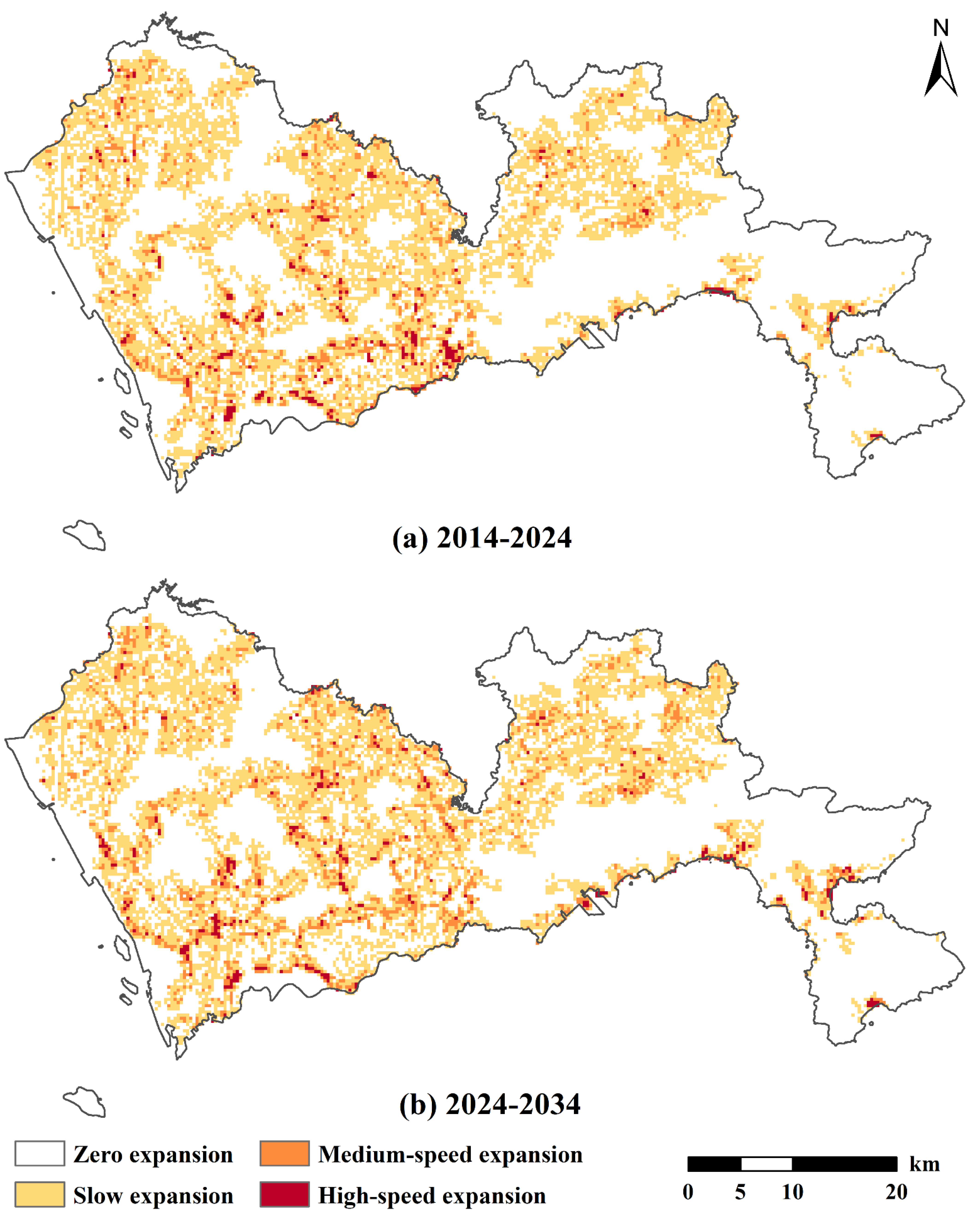
5.2. D Expansion Analysis

Grid analysis is a spatial measurement method that calculates each grid within the study area by arranging uniform grids in the entire area and using such grids as the basic unit to reflect the spatial heterogeneity of urban expansion [49]. We selected a 300 m × 300 m grid to cover the study area and used it to calculate the urban 3D expansion intensity index within each grid. We used the natural fracture method to divide the index into four levels: high-speed expansion, medium-speed expansion, slow expansion, and zero expansion.
The spatial distribution of urban 3D expansion intensity in Shenzhen from 2014 to 2034 is shown in Figure 13. The distribution of expansion intensity in Shenzhen was consistent in 2014–2024 and 2024–2034. Shenzhen was characterized mainly by low-speed expansion. Expansions occurred in all areas except mountainous areas. High-speed expansion was mainly concentrated in the southern downtown and economically developed areas. Areas of high-speed expansion from 2014 to 2024 were mainly concentrated in eastern Luohu, Futian Nanshan, and Longhua. The expansion intensity from 2024 to 2034 changed slightly. The intensity of Dapeng and northern Shenzhen increased. By contrast, the intensity of the northern city center slightly decreased, especially in the southern part of Luohu, which had high-speed and medium-speed expansion and later shifted to medium- and low-speed expansion. The central of Nanshan and Baoan showed a slight increase in intensity and high-speed areas. The high-speed expansion area of Dapeng increased slightly.
In addition, we analyzed the urban 3D expansion intensity of urban land use types in Shenzhen via grid analysis. Figure 14 shows the spatial distribution of the 3D expansion intensities of public management services land, commercial land, residential land, and industrial land from 2014 to 2034. The spatial distribution of the expansion intensity of each urban land type in 2014–2024 and 2024–2034 was still relatively consistent and dominated by low-speed expansion. The expansion intensity of public management services land was high in the south-central area near the city center. The three areas around Tiegang Reservoir (Baoan), Shenzhen Bay (Futian), and Donghu Park (Luohu) are hotspots of high-speed expansion. Commercial land had a high expansion intensity in Nanshan and the northern coastal area of Dapeng. High-speed expansion hotspots were also located here. The expansion of residential land was extensive. The area around the Shenzhen North Station (Longhua) was a high-speed expansion hotspot. Industrial land expansion was the most extensive and mainly concentrated in the north. High-speed expansion hotspots were scattered, with scant distribution in the downtown area.

6. Conclusions

This paper proposed an urban 3D spatial expansion simulation model. The model combined the FLUS model to simulate urban land use changes in the horizontal direction and RF regression to predict building height growth in the vertical direction. A synergistic simulation of urban horizontal expansion and vertical growth was realized.
The proposed model simulated urban land use in the horizontal direction with good accuracy (kappa = 0.91, OA = 0.95, FoM = 0.19) and effectiveness. The prediction of building height modelling based on RF regression had a good fitting accuracy and low relative error. Building height growth is driven by many spatial factors. Among them, the location factor had the highest contribution and was the primary factor influencing building height growth. Spatial factors of socioeconomic and location advantages drove building heights to change much Topographic factors had a low contribution and played a limited role in constraining building height growth.
We simulated urban 3D spatial changes in Shenzhen from 2014 to 2034 using the proposed model. Industrial land expanded extensively, especially in the northern Shenzhen, with mainly new low-rise buildings. Public management services expanded significantly in the city centre (Nanshan, Futian, and Luohu), mainly adding new low-rise and medium-rise buildings. Commercial land expanded significantly in Nanshan, Baoan, and Dapeng, with mainly new low-rise and medium-rise buildings and a small number of new high-rise buildings. Residential land expanded significantly around Shenzhen North Station within Longhua, mostly with low-rise and medium-rise building developments. The distribution of expansion intensity in Shenzhen was consistent in 2014–2024 and 2024–2034. Urban land is dominated by low-speed expansion. High-speed expansion was mainly concentrated in the southern city center and economically developed areas. Differences in expansion scope, expansion intensity distribution, and high-speed expansion hotspot areas were obvious for different urban lands.
The building height modelling in this study can identify the crucial factors affecting building height changes and improve the mining and analysis of the driving mechanism of urban 3D spatial expansion. The proposed urban 3D spatial expansion simulation model can synergistically simulate horizontal and vertical growth. The analysis of 3D spatial expansion results can identify hotspot areas for future urban 3D expansion. This study solves the problem of the absence of simulation and analysis of real cities in urban 3D simulations and expands and improves urban 3D simulation research.
In further research, multi-period building height data can be considered for the calibration and validation of urban vertical growth simulations to improve the evaluation and accuracy of urban vertical growth simulation. Accurately simulating urban 3D spatial structure changes in urban 3D simulation studies is difficult and requires data sources of higher quality and accuracy than those used in this study. The highly accurate 3D building model information and refined urban spatial big data in the city information model can be used to enrich data sources for urban 3D simulation and then accurately simulate and explore 3D spatial change patterns and characteristics of cities.

Author Contributions

Conceptualization, Methodology, L.Z., X.L. and X.X.; Software, Data curation, Validation, Formal analysis, Resources, Visualization, Writing—Original Draft, Writing—Review and Editing, L.Z.; Resources, Supervision, Project Administration, X.L.; Funding Acquisition, X.L., X.X., C.L. and K.C. All authors have read and agreed to the published version of the manuscript.

Funding

This research was supported by the National Key Research & Development Program of China (Grant No. 2019YFA0607203), the National Natural Science Foundation of China (Grant No. 42171409, 42001326), and the Guangdong Enterprise Key Laboratory for Urban Sensing, Monitoring and Early Warning (Grant No. 2020B121202019) and The Science and Technology Foundation of Guangzhou Urban Planning & Design Survey Research Institute (RD No. RDI2210201071, RDI2210201143).

Data Availability Statement

The original land use data that support the findings of this study was provided by the Bureau of Land and Resources of Shenzhen, and cannot be made publicly available to protect the data confidentiality. If necessary, the data can be applied with the Shenzhen Planning and Natural Resources Bureau. All other data are acquired from public data sources listed in the main content with references.

Conflicts of Interest

The authors declare no conflict of interests.

References

  1. Li, X.; Chen, G.; Liu, X.; Liang, X.; Wang, S.; Chen, Y.; Pei, F.; Xu, X. A New Global Land-Use and Land-Cover Change Product at a 1-km Resolution for 2010 to 2100 Based on Human–Environment Interactions. Ann. Am. Assoc. Geogr. 2017, 107, 1040–1059. [Google Scholar] [CrossRef]
  2. Rao, Y.; Zhou, J.; Zhou, M.; He, Q.; Wu, J. Comparisons of three-dimensional urban forms in different urban expansion types: 58 sample cities in China. Growth Chang. 2020, 51, 1766–1783. [Google Scholar] [CrossRef]
  3. Koziatek, O.; Dragićević, S. iCity 3D: A geosimualtion method and tool for three-dimensional modeling of vertical urban development. Landsc. Urban Plan. 2017, 167, 356–367. [Google Scholar] [CrossRef]
  4. Yeh, A.G.-O.; Li, X. Economic development and agricultural land loss in the Pearl River Delta, China. Habitat Int. 1999, 23, 373–390. [Google Scholar] [CrossRef]
  5. Li, B.; Liu, Z.; Nan, Y.; Li, S.; Yang, Y. Comparative Analysis of Urban Heat Island Intensities in Chinese, Russian, and DPRK Regions across the Transnational Urban Agglomeration of the Tumen River in Northeast Asia. Sustainability 2018, 10, 2637. [Google Scholar] [CrossRef] [Green Version]
  6. Bürgi, M.; Hersperger, A.M.; Schneeberger, N. Driving forces of landscape change—Current and new directions. Landsc. Ecol. 2004, 19, 857–868. [Google Scholar] [CrossRef]
  7. Su, S.; Jiang, Z.; Zhang, Q.; Zhang, Y. Transformation of agricultural landscapes under rapid urbanization: A threat to sustainability in Hang-Jia-Hu region, China. Appl. Geogr. 2011, 31, 439–449. [Google Scholar] [CrossRef]
  8. Frolking, S.; Milliman, T.; Seto, K.C.; Friedl, M.A. A global fingerprint of macro-scale changes in urban structure from 1999 to 2009. Environ. Res. Lett. 2013, 8, 024004. [Google Scholar] [CrossRef]
  9. Kuang, W.; Liu, J.; Zhang, Z.; Lu, D.; Xiang, B. Spatiotemporal dynamics of impervious surface areas across China during the early 21st century. Chin. Sci. Bull. 2013, 58, 1691–1701. [Google Scholar] [CrossRef] [Green Version]
  10. Li, X.; Liu, X. An extended cellular automaton using case-based reasoning for simulating urban development in a large complex region. Int. J. Geogr. Inf. Sci. 2006, 20, 1109–1136. [Google Scholar] [CrossRef]
  11. Wu, F.; Webster, C.J. Simulation of land development through the integration of cellular automata and multicriteria evaluation. Environ. Plan. B Plan. Des. 1998, 25, 103–126. [Google Scholar] [CrossRef]
  12. Liu, X.; Li, X.; Liu, L.; He, J.; Ai, B. A bottom-up approach to discover transition rules of cellular automata using ant intelligence. Int. J. Geogr. Inf. Sci. 2008, 22, 1247–1269. [Google Scholar] [CrossRef]
  13. Li, X.; Yang, Q.; Liu, X. Discovering and evaluating urban signatures for simulating compact development using cellular automata. Landsc. Urban Plan. 2008, 86, 177–186. [Google Scholar] [CrossRef]
  14. Shirley, L.J.; Battaglia, L.L. Projecting Fine Resolution Land-Cover Dynamics for a Rapidly Changing Terrestrial–Aquatic Transition in Terrebonne Basin, Louisiana, U.S.A. J. Coast. Res. 2008, 2008, 1545–1554. [Google Scholar] [CrossRef]
  15. Li, X.; Yeh, A.G.-O. Data mining of cellular automata’s transition rules. Int. J. Geogr. Inf. Sci. 2004, 18, 723–744. [Google Scholar] [CrossRef]
  16. Rienow, A.; Stenger, D.; Menz, G. Sprawling cities and shrinking regions—Forecasting urban growth in the RUHR for 2025 by coupling cells and agents. Erdkunde 2014, 68, 85–107. [Google Scholar] [CrossRef]
  17. Chen, Y.; Li, X.; Liu, X.; Ai, B. Modeling urban land-use dynamics in a fast developing city using the modified logistic cellular automaton with a patch-based simulation strategy. Int. J. Geogr. Inf. Sci. 2014, 28, 234–255. [Google Scholar] [CrossRef]
  18. Wu, F. Calibration of stochastic cellular automata: The application to rural-urban land conversions. Int. J. Geogr. Inf. Sci. 2002, 16, 795–818. [Google Scholar] [CrossRef]
  19. Li, X.; Yeh, A.G. Calibration of cellular automata by using neural networks for the simulation of complex urban systems. Environ. Plan. A 2001, 33, 1445–1462. [Google Scholar] [CrossRef]
  20. He, J.; Li, X.; Yao, Y.; Hong, Y.; Zhang, J. Mining transition rules of cellular automata for simulating urban expansion by using the deep learning techniques. Int. J. Geogr. Inf. Sci. 2018, 32, 2076–2097. [Google Scholar] [CrossRef]
  21. Zhang, D.; Liu, X.; Wu, X.; Yao, Y.; Wu, X.; Chen, Y. Multiple intra-urban land use simulations and driving factors analysis: A case study in Huicheng, China. GISci. Remote Sens. 2019, 56, 282–308. [Google Scholar] [CrossRef]
  22. Liu, X.; Liang, X.; Li, X.; Xu, X.; Ou, J.; Chen, Y.; Li, S.; Wang, S.; Pei, F. A future land use simulation model (FLUS) for simulating multiple land use scenarios by coupling human and natural effects. Landsc. Urban Plan. 2017, 168, 94–116. [Google Scholar] [CrossRef]
  23. Benguigui, L.; Czamanski, D.; Roth, R. Modeling Cities in 3D: A Cellular Automaton Approach. Environ. Plan. B Plan. Des. 2008, 35, 413–430. [Google Scholar] [CrossRef]
  24. Qin, J.; Fang, C.; Wang, X. The Three-dimensional Urban Growth Simulating Based on Cellular Automata. J. Geo-Inf. Sci. 2013, 15, 662–671. [Google Scholar] [CrossRef]
  25. Lin, J.; Huang, B.; Chen, M.; Huang, Z. Modeling urban vertical growth using cellular automata—Guangzhou as a case study. Appl. Geogr. 2014, 53, 172–186. [Google Scholar] [CrossRef]
  26. He, Q.; Liu, Y.; Zeng, C.; Yin, C.; Tan, R. Simultaneously simulate vertical and horizontal expansions of a future urban landscape: A case study in Wuhan, Central China. Int. J. Geogr. Inf. Sci. 2017, 31, 1907–1928. [Google Scholar] [CrossRef]
  27. Yao, Y.; Zhang, J.; Hong, Y.; Liang, H.; He, J. Mapping fine-scale urban housing prices by fusing remotely sensed imagery and social media data. Trans. GIS 2018, 22, 561–581. [Google Scholar] [CrossRef]
  28. Qin, J.; Fang, C.; Fang, Y.; Li, G.; Wang, S. Evaluation of three-dimensional urban expansion: A case study of Yangzhou City, Jiangsu Province, China. Chin. Geogr. Sci. 2015, 25, 224–236. [Google Scholar] [CrossRef]
  29. Yao, Y.; Liu, X.; Li, X.; Liu, P.; Hong, Y.; Zhang, Y.; Mai, K. Simulating urban land-use changes at a large scale by integrating dynamic land parcel subdivision and vector-based cellular automata. Int. J. Geogr. Inf. Sci. 2017, 31, 2452–2479. [Google Scholar] [CrossRef]
  30. Huang, Y.; Liu, Y.; Lieske, S. Modeling and Predicting Vertical Urban Growth: An Exploratory Review. GeoComputation. 2019. Available online: https://auckland.figshare.com/articles/conference_contribution/Detecting_Modeling_and_Predicting_Vertical_Urban_Growth_An_exploratory_review/9863141/2 (accessed on 14 February 2022). [CrossRef]
  31. Lin, J.; Wan, H.; Cui, Y. Analyzing the spatial factors related to the distributions of building heights in urban areas: A comparative case study in Guangzhou and Shenzhen. Sustain. Cities Soc. 2020, 52, 101854. [Google Scholar] [CrossRef]
  32. Liang, X.; Liu, X.; Li, X.; Chen, Y.; Tian, H.; Yao, Y. Delineating multi-scenario urban growth boundaries with a CA-based FLUS model and morphological method. Landsc. Urban Plan. 2018, 177, 47–63. [Google Scholar] [CrossRef]
  33. Chen, G.; Li, X.; Liu, X.; Chen, Y.; Liang, X.; Leng, J.; Xu, X.; Liao, W.; Qiu, Y.; Wu, Q.; et al. Global projections of future urban land expansion under shared socioeconomic pathways. Nat. Commun. 2020, 11, 537. [Google Scholar] [CrossRef] [PubMed] [Green Version]
  34. Liao, W.; Liu, X.; Xu, X.; Chen, G.; Liang, X.; Zhang, H.; Li, X. Projections of land use changes under the plant functional type classification in different SSP-RCP scenarios in China. Sci. Bull. 2020, 65, 1935–1947. [Google Scholar] [CrossRef]
  35. Liang, X.; Liu, X.; Li, D.; Zhao, H.; Chen, G. Urban growth simulation by incorporating planning policies into a CA-based future land-use simulation model. Int. J. Geogr. Inf. Sci. 2018, 32, 2294–2316. [Google Scholar] [CrossRef]
  36. Liang, X.; Liu, X.; Chen, G.; Leng, J.; Wen, Y.; Chen, G. Coupling fuzzy clustering and cellular automata based on local maxima of development potential to model urban emergence and expansion in economic development zones. Int. J. Geogr. Inf. Sci. 2020, 34, 1930–1952. [Google Scholar] [CrossRef]
  37. Liu, X.; Hu, G.; Ai, B.; Li, X.; Tian, G.; Chen, Y.; Li, S. Simulating urban dynamics in China using a gradient cellular automata model based on S-shaped curve evolution characteristics. Int. J. Geogr. Inf. Sci. 2018, 32, 73–101. [Google Scholar] [CrossRef]
  38. Wu, X.; Liu, X.; Liang, X.; Chen, G. Multi-scenarios Simulation of Urban Growth Boundaries in Pearl River Delta Based on FLUS-UGB. J. Geo-Inf. Sci. 2018, 20, 532–542. [Google Scholar]
  39. Zhao, L.; Liu, X.; Liu, P.; Chen, G.; He, J. Urban Expansion Simulation and Early Warning based on Geospatial Partition and FLUS Model. J. Geo-Inf. Sci. 2020, 22, 517–530. [Google Scholar]
  40. Breiman, L. Random Forests. Mach. Learn. 2001, 45, 5–32. [Google Scholar] [CrossRef] [Green Version]
  41. He, S.; Wang, X.; Dong, J.; Wei, B.; Duan, H.; Jiao, J.; Xie, Y. Three-Dimensional Urban Expansion Analysis of Valley-Type Cities: A Case Study of Chengguan District, Lanzhou, China. Sustainability 2019, 11, 5663. [Google Scholar] [CrossRef] [Green Version]
  42. Pontius, R.G.; Cornell, J.D.; Hall, C.A.S. Modeling the spatial pattern of land-use change with GEOMOD2: Application and validation for Costa Rica. Agric. Ecosyst. Environ. 2001, 85, 191–203. [Google Scholar] [CrossRef] [Green Version]
  43. Jr, R.G.P.; Millones, M. Death to Kappa: Birth of quantity disagreement and allocation disagreement for accuracy assessment. Int. J. Remote Sens. 2011, 32, 4407–4429. [Google Scholar] [CrossRef]
  44. Liu, X.; Li, X.; Shi, X.; Wu, S.; Liu, T. Simulating complex urban development using kernel-based non-linear cellular automata. Ecol. Model. 2008, 211, 169–181. [Google Scholar] [CrossRef]
  45. Jr, R.G.P.; Walker, R.; Yao-Kumah, R.; Arima, E.; Aldrich, S.; Caldas, M.; Vergara, D. Accuracy Assessment for a Simulation Model of Amazonian Deforestation. Ann. Assoc. Am. Geogr. 2007, 97, 677–695. [Google Scholar] [CrossRef]
  46. Hu, Z.; Du, P.; Guo, D. Analysis of Urban Expansion and Driving Forces in Xuzhou City Based on Remote Sensing. J. China Univ. Min. Technol. 2007, 17, 267–271. [Google Scholar] [CrossRef]
  47. Fan, F.; Wang, Y.; Qiu, M.; Wang, Z. Evaluating the Temporal and Spatial Urban Expansion Patterns of Guangzhou from 1979 to 2003 by Remote Sensing and GIS Methods. Int. J. Geogr. Inf. Sci. 2009, 23, 1371–1388. [Google Scholar] [CrossRef]
  48. Pontius, R.G.; Boersma, W.; Castella, J.-C.; Clarke, K.; de Nijs, T.; Dietzel, C.; Duan, Z.; Fotsing, E.; Goldstein, N.; Kok, K.; et al. Comparing the input, output, and validation maps for several models of land change. Ann. Reg. Sci. 2008, 42, 11–37. [Google Scholar] [CrossRef] [Green Version]
  49. Zhao, J.; Chen, H.; Xu, H. A Study on the Intensity and Spatial Pattern of Urban Residential Growth in Shanghai from 1947 to 2002. J. Nat. Resour. 2005, 20, 400–406. [Google Scholar]
Figure 1. Case study area: Shenzhen, Guangdong Province, China.
Remotesensing 14 01503 g001
Figure 2. Urban land use data of Shenzhen in 2009 and 2014. Where (AC) represent their respective regions, respectively; (A1,A2) represent the urban land use of region A in 2009 and 2014; (B1,B2) represent the urban land use of region B in 2009 and 2014; (C1,C2) represent the urban land use of region C in 2009 and 2014.
Remotesensing 14 01503 g002
Figure 3. Spatial distribution of building heights in Shenzhen. (a) The central region of Nanshan District; (b) The central region of Futian District; (c) The southwestern region of Luohu District.
Remotesensing 14 01503 g003
Figure 4. Driving factors of urban land use change in Shenzhen. (a) DEM; (b) slope; (c) distance to city center; (d) distance to district centers; (e) distance to railways; (f) distance to highways; (g) distance to national roads; (h) distance to provincial roads; (i) distance to railway stations; (j) distance to subway stations; (k) distance to ocean; (l) distance to lakes; (m) distance to rivers; (n) density of urban road network; (o) population density; (p) PM2.5; (q) GDP.
Remotesensing 14 01503 g004
Figure 5. Spatial factors of building heights in Shenzhen. (a) DEM; (b) slope; (c) distance to parks and green spaces; (d) distance to waters; (e) housing prices; (f) density of entertainment facilities; (g) density of supermarkets; (h) density of restaurants; (i) density of factories; (j) density of shopping malls; (k) population density; (l) density of hospitals; (m) nighttime light intensity; (n) distance to city center; (o) distance to district centers; (p) distance to urban roads; (q) density of bus stations.
Remotesensing 14 01503 g005
Figure 6. Flowchart of urban 3D spatial expansion simulation model.
Remotesensing 14 01503 g006
Figure 7. Framework of CA in FLUS model.
Remotesensing 14 01503 g007
Figure 8. Actual and simulated land use patterns in Shenzhen in 2014. Where (AC) represent their respective regions, respectively; (A1,A2) represent the actual and simulated land use patterns in region A; (B1,B2) represent the actual and simulated land use patterns in region B; (C1,C2) represent the actual and simulated land use patterns in region C.
Remotesensing 14 01503 g008
Figure 9. Spatial distribution of relative errors between actual and predicted FAR. (A) The northern region of Longhua District; (B) The southeastern region of Futian District.
Remotesensing 14 01503 g009
Figure 10. Ratio of the interval range of the relative error between actual and predicted FAR.
Remotesensing 14 01503 g010
Figure 11. Simulated urban land use patterns of Shenzhen in the horizontal direction, 2014–2034. (A) The region near Shenzhen Bay; (B) The region near the Shenzhen North Railway Station in the south of Longhua District; (A1A3) represent the urban land use patterns of region A in 2014, 2024 and 2034; (B1B3) represent the urban land use patterns of region B in 2014, 2024 and 2034.
Remotesensing 14 01503 g011
Figure 12. Predicted results of building height growth of Shenzhen in the vertical direction, 2014–2034. (A) The region near Shenzhen Bay; (B) The region near the Shenzhen North Railway Station in the south of Longhua District; (A1A3) represent the predicted results of building height growth of region A in 2014, 2024 and 2034; (B1B3) represent the predicted results of building height growth of region B in 2014, 2024 and 2034.
Remotesensing 14 01503 g012
Figure 13. (a) The spatial distribution of urban 3D expansion intensity in Shenzhen from 2014 to 2024; (b) The spatial distribution of urban 3D expansion intensity in Shenzhen from 2024 to 2034.
Remotesensing 14 01503 g013
Figure 14. Spatial distribution of urban 3D expansion intensity of urban land use types in Shenzhen, 2014–2034. (a) public management services land; (b) commercial land; (c) residential land; (d) industrial land.
Remotesensing 14 01503 g014
Table 1. List of data used in this study.
CategoryDataYearResolutionData Resource
Basic geographic information dataAdministrative boundaries, city center, district centers, river, lake, ocean, railway stations, subway stations2015 National Catalogue Service for Geographic Information
Parks and green spaces2020 OpenStreetMap
DEM2000–201330 mASTER GDEM V3
Slope 30 mCalculated from DEM
Socioeconomic dataGDP20151 kmResource and Environment Science and Data Center, Chinese Academy of Sciences
Population2015100 mWorld pop
Nighttime light intensity201515″
(450 m)
NOAA/NGDC—EOG
Housing prices20175 m[27]
Climate and environmental dataPM2.52014–20160.01°
(1.11 km)
SEDAC
Land use dataFine cadastral land use2009, 2014 Bureau of Land and Resources of Shenzhen
Building dataBuilding heights2016 Gaode Map API
Points of interestShopping malls, hospitals, entertainment facilities, supermarkets, restaurants, parks, bus stations, factories2016 Gaode Map API
All levels of road dataHighway, railway, national road, provincial road, urban road network2020 OpenStreetMap
Table 2. Total conversion area (km2) of different land use types in Shenzhen from 2009 to 2014.
2014NPCRI
2009
N1368.503014.55395.524910.686516.7462
P6.499385.79410.00000.01830.0152
C0.35680.013726.04100.00050.0000
R0.25590.00050.0000187.88870.0007
I3.75330.26850.01060.0047266.4813
Table 3. Total simulated area (km2) of each land use type under future years.
Land Use Types20242034
Non-construction land (N)1313.73721253.2788
Public management services land (P)110.6550121.6656
Commercial land (C)40.192248.8844
Residential land (R)219.6963238.7700
Industrial land (I)309.0222330.7032
Table 4. Volume demand for each urban land expansion under future years.
Urban Land Types20242034
Public management services land (P)181.2678199.3047
Commercial land (C)101.7893123.8028
Residential land (R)520.0457565.1953
Industrial land (I)538.8655576.6723
Table 5. Contribution weights of spatial factors on buildings’ FAR.
Spatial FactorsContribution Weights
DEM5.09%
Slope4.93%
Distance to parks and green spaces6.21%
Distance to waters5.46%
Housing prices6.15%
Density of entertainment facilities6.41%
Density of supermarkets6.17%
Density of restaurants6.39%
Density of factories3.55%
Density of shopping malls6.09%
Population density5.52%
Density of hospitals6.44%
Nighttime light intensity5.26%
Distance to city center7.35%
Distance to district centers6.59%
Distance to urban roads6.12%
Density of bus stations6.30%
Publisher’s Note: MDPI stays neutral with regard to jurisdictional claims in published maps and institutional affiliations.

