Article

Evaluation of the Influence of Processing Parameters in Structure-from-Motion Software on the Quality of Digital Elevation Models and Orthomosaics in the Context of Studies on Earth Surface Dynamics

by
Szymon Śledź
* and
Marek W. Ewertowski
Faculty of Geographical and Geological Sciences, Adam Mickiewicz University, Krygowskiego 10, 61-680 Poznań, Poland
*
Author to whom correspondence should be addressed.
Remote Sens. 2022, 14(6), 1312; https://doi.org/10.3390/rs14061312
Submission received: 26 January 2022 / Revised: 3 March 2022 / Accepted: 7 March 2022 / Published: 9 March 2022
(This article belongs to the Special Issue Recent Advances in GIS Techniques for Remote Sensing)

Abstract

:
The fully automated Structure-from-Motion approach for developing digital elevation models and orthomosaics has been known and used in photogrammetry for at least 15 years. Years of practice and experience have allowed researchers to provide a solid description of the applicability and limitations of this method. That being said, the impact of input processing parameters in software on the quality of photogrammetric products has yet to be fully ascertained empirically. This study is aimed at identifying the most advantageous processing workflow to fill this research gap by testing 375 different setup variations in the Agisoft Metashape software for the same set of images acquired using an unmanned aerial vehicle in a proglacial area. The purpose of the experiment was to determine three workflows: (1) the fastest, which has the shortest calculation time; (2) the best quality, which is as accurate as possible, regardless of the time taken for the calculations; and (3) the optimal, which is a compromise between accuracy and calculation time. Each of the 375 processing setup variations was assessed based on final product accuracy, i.e., orthomosaics and digital elevation models. The three workflows were selected based on calculating the height differences between the digital elevation models and the control points that did not participate in their georeferencing. The analyses of the root mean square errors (RMSE) and standard deviations indicate that excluding some of the optimization parameters during the camera optimization stage results in high RMSE and an increase in the values of standard deviation errors. Furthermore, it was shown that increasing the detail of individual processing steps in software does not always positively affect the accuracy of the resulting models. The experiment resulted in the development of three different workflows in the form of Python scripts for Agisoft Metashape software, which will help users to process image sets efficiently in the context of earth surface dynamics studies.

1. Introduction

The relief of the Earth’s surface is constantly modified by natural processes (e.g., erosion, weathering) and direct human activity. These dynamics are important to studies of the landscape evolution as well as studies of processes which may pose threats to human life and infrastructure. Therefore, landscape dynamics have been studied in a number of contexts that include the following: (a) the possibility of the occurrence of landslides and areas susceptible to their formation [1,2,3]; (b) to observe areas at risk of snow avalanches [4]; (c) to monitor land surface changes due to mining activities [5,6]; and (d) to assess the dynamics of aeolian processes [7] or changes to riverscapes [8,9,10,11,12]. One example of areas characterized by particularly high dynamics of the surface is proglacial areas [13,14,15,16,17]. Ongoing climate warming [18,19,20], characterized by an increase in mean annual air temperatures and changes in precipitation, causes the melting of glaciers [21] and reveals numerous geomorphological forms in their forelands, previously hidden under the glacier ice [20,22,23,24]. Moreover, proglacial areas are an important storage of water (in the form of dead-ice) and sediments, which can be relatively easy to mobilize [20,25,26]. For example, meltwaters often have a significant erosive potential and can cause large transformations both in the immediate foreland of the glaciers and in the areas further away, through glacier lake outburst floods or debris flows [11,27,28,29,30,31]. For this reason, proglacial areas are currently the subject of research by many scientists who use modern research techniques to monitor and collect data on land surface characteristics and landform dynamics in front of retreating glaciers worldwide [17].
Unmanned aerial vehicles (UAV, drone), equipped with a sensor in the form of an RGB camera, have recently become a popular platform for observing various objects or areas from above [32,33,34]. The undoubted advantage of UAVs in environmental research is low price, mobility and high configuration options, depending on the model and manufacturer. Anderson and Gaston rightly noticed in 2013 [35] that UAVs will revolutionize spatial ecology—UAVs can now be found in more and more applications related to scientific and commercial activities. Thanks to the UAV, the operator can take images of the selected research objects from a low altitude while performing a manual or autonomous flight. A dedicated UAV application allows for setting up parameters such as flight altitude, flight speed, forward and side overlap of images, or marking the area of interest and designing the mission path. The current mobile applications significantly support the operator during a mission, e.g., automatically interrupting it when the battery is low and warning against bad weather conditions such as strong gusts of wind. In glacial geomorphology, UAVs have been widely used since 2010, and different studies utilized various UAV construction types, sensors, and flight parameters, depending on the shape of the studied area, meteorological conditions, research objectives and the expected accuracy of photogrammetric products [12,36,37]. It should be emphasized that in addition to aerial images obtained from UAVs, images collected from terrestrial photogrammetry (robotic or stationary) are becoming more and more popular (e.g., [38]).
The end result of the survey mission is a collection of images, which is a record of the current state of the studied area. The images can be used as photographic documentation, but primarily as data for the development of a digital elevation model (DEM) and orthomosaic as the end products of processing in Structure-from-Motion (SfM) software [39]. Thanks to the external Ground Control Points (GCPs), measured with the differential Global Navigation Satellite Systems (dGNSS) receiver (external georeferencing) or the lo-cations embedded in the images from the on-board GNSS receiver (direct georeferencing, which can also be replaced by corrected camera positions as a text file imported to the software), the SfM software combines the images with each other based on characteristic points, marked on at least two images. As a result, first a sparse, and then a dense point cloud is obtained, which is the basis for generating the final photogrammetric products. A DEM, which is a three-dimensional model of the studied area’s surface and orthomosaic, is commonly used for analyses related to geomorphological mapping (e.g., [22,28,40,41,42]), change detection (e.g., [38,43,44,45]), process-form studies [46] or mapping of surficial geology [47]. Evidence of the common use of UAV and the SfM method in geomorphology consists of publications in which the authors present the appropriate workflow of conduct during field research and in the further preparation of publications and presentation of results (e.g., [48,49,50]). Thus far, however, it has not been tested in detail how individual processing parameters in the SfM software affect the accuracy of the final result. Selection of the appropriate parameters is important because this stage has a crucial impact on the accuracy of the models obtained, which, if performed incorrectly, may lead to wrong results and thus incorrect conclusions from the conducted research.
Thus far, only limited publications have attempted to explain the influence of different calculation methods on the accuracy of photogrammetric products and possible ways to accelerate the processing of UAV-generated images into DEMs and orthomosaics. For example, some attention was directed to the impact of mission design (e.g., [51,52,53]) or number and location of GCPs (e.g., [54,55,56,57]) on the accuracy of photogrammetric products. Another example is a work illustrating the processing of photo sets with no GCPs, but using co-registrations of the models (e.g., [58]). The authors proved that in this type of research, such as change detection, satisfactory results can be achieved even without GCPs, which is particularly important in the case of objects that are difficult to access. Similar conclusions were suggested by de Haas et al. [59], who presented evidence for the limited impact of GCPs on the increase in accuracy of models compared to projects where the co-alignment of multiple surveys is used. In addition, researchers also checked if the choice of software matters for the quality of DSM (e.g., [60]) and application of oblique photos (e.g., [61]), and critically assessed the use of RTK technology in UAVs compared to the traditional GCP scheme with UAVs without this technology [62]. The aim of this study was to investigate the influence of particular calculation parameters in the Agisoft Metashape software on the accuracy of photogrammetric products: DEMs and orthomosaics. Another objective was to find the most efficient workflows that can be used in the processing of large images sets of different research objects. For this purpose, 375 different workflows were formulated in the software, which were then checked while processing the same set of images representative of the proglacial area. Additionally, we aimed to select three workflows: (1) the fastest, which has the shortest calculation time; (2) the best quality, which is as accurate as possible, regardless of the time taken for calculations; and (3) the optimal, which is a compromise between accuracy and calculation time. These workflows are included in this article as Supplementary Materials in the form of Python scripts for processing a set of images in Agisoft Metashape. Thus far, there is no publication of such multi-threaded research in that form that can be easily implemented by other researchers in their work. The correct selection of the script and processing efficiency depend on the size of the image set, the expected accuracy, or the available computing power.

2. Materials and Methods

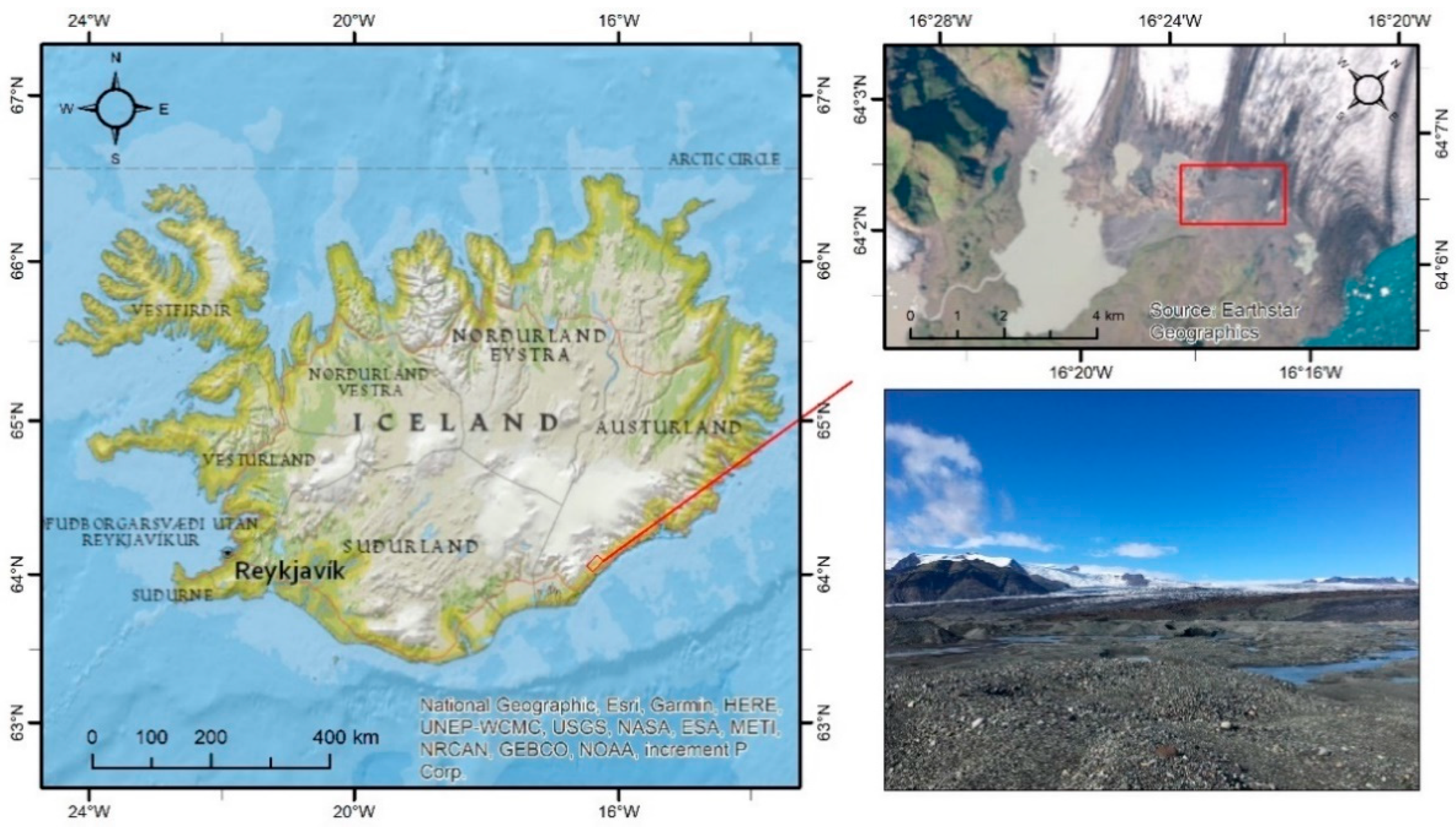
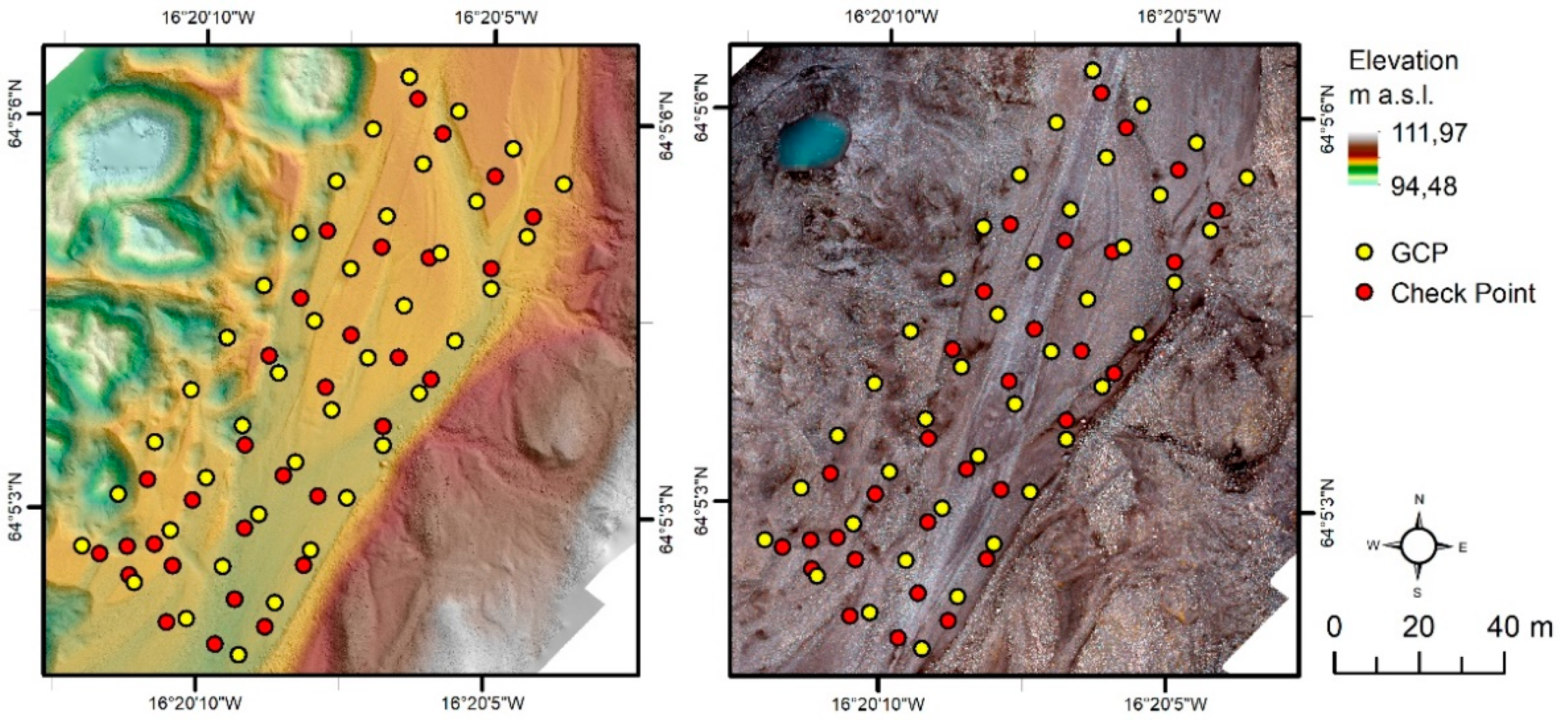
2.1. Study Area and Technical Information

The experiment used a set of UAV-collected images showing a sample area (~50,000 m2) of diverse terrain within the foreland of the Breiðamerkurjökull, Iceland (Figure 1). The flight took place on 5 September 2021 using the Map Pilot Pro mobile application in autonomous mode. To acquire the images, we used a multirotor DJI Phantom 4 Pro UAV equipped with a DJI FC6310 camera at a resolution of 20 MP and a focal length of 8.8 mm (24 mm equivalent for 35 mm format). In total, 82 vertical RAW images with a resolution of 5464 × 3640 pixels were taken and saved in the DNG format. The forward and side overlap were programmed at 80%, while the flight altitude was set at 70 m, rate of the image capture: ~5 s. The photographic exposure was set at 1/160 s (19 images) and 1/120 s (63 images). The GSD (Ground Sample Distance) of the images was ~1.92 cm/pix. The intention of the authors was to carefully reproduce the typical settings for missions performed for similar purposes [37]. During the flight, no strong gusts of wind or rainfall were noticed, even though the sky was fully cloudy. The quality of the images was checked in the Agisoft Metashape software before processing using a dedicated tool “Estimate image quality”—each image taken for calculations had a value above 0.80. DNG images were directly imported into Agisoft Metashape and were not subjected to exposure nor color modifications.
We used 40 GCPs, arranged in 4 rows of 10 points and 15 m apart at an angle of 90°, to georeference the model. Additionally, in order to check the accuracy of DEMs, 31 control points (CPs) not involved in georeferencing during SfM processing were randomly located in the study area. Each of the GCPs and CPs were constructed in the form of a circle of stones, in which the location of the middle stone was measured by the differential GNSS Topcon Hiper II receiver (Figure 2), using RTK survey technique and local base station (vector < 200 m). Survey uncertainties were between 0.008 and 0.015 m. The Agisoft Metashape Professional software (version 1.7.1 build 11,797) was used to process the set of images, model and generate DEMs and orthomosaics. The computing platform was a desktop computer with Windows 10 64 bit, a 6-core (12 thread) Intel Xeon E5-2440 processor with a base frequency of 2.40 GHz (2.90 GHz in Turbo mode), a GeForce GTX 1060 6 GB graphics card, and 79.97 GB DDR3 RAM. The computer was not used for other purposes during calculations to ensure the same computing power for all models.

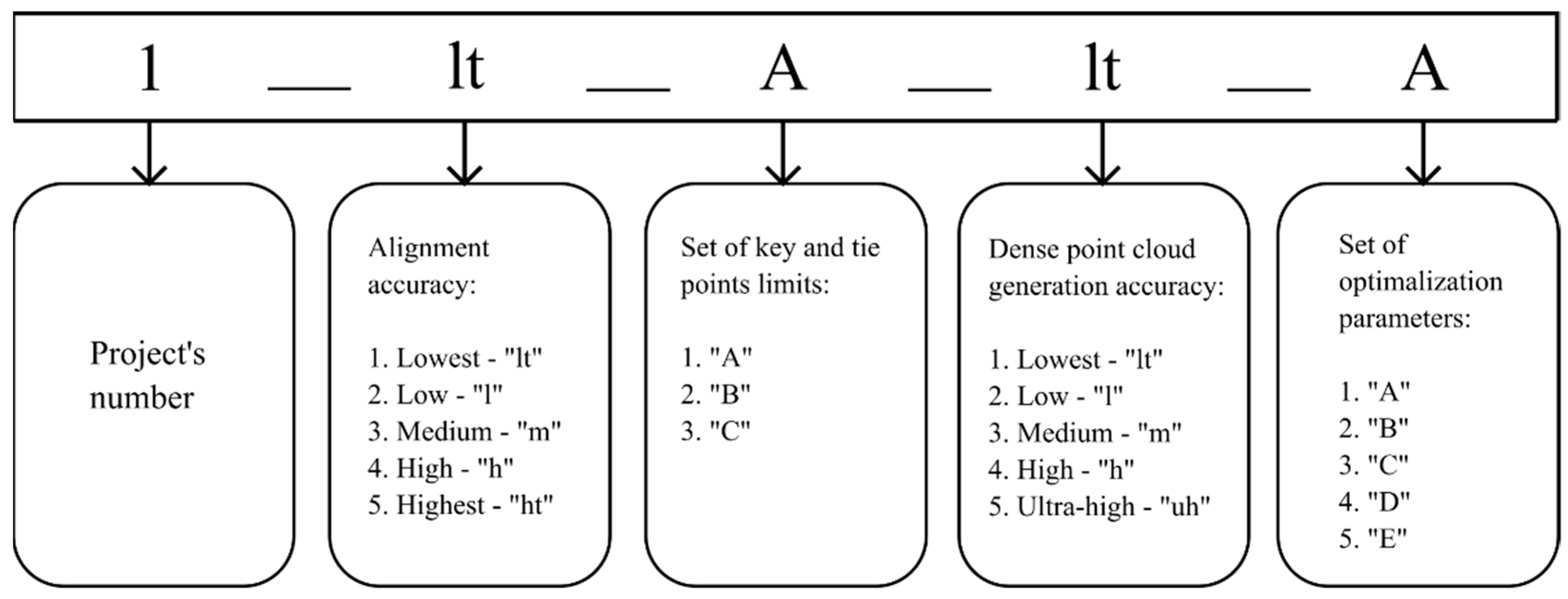
2.2. Guidelines of the Experiment

Before starting the calculations, the planned variants of input processing parameters were formulated in the software, while naming of the projects followed a logical, structured and individual code (Figure 3). We investigated how the following parameters and their values would impact the final accuracy of the photogrammetric products (measured by errors on CPs) and calculation time:
  • Alignment accuracy—five levels of accuracy: lowest, low, medium, high, and highest.
  • The number of key points and tie—three sets were adopted:
    • Set “A”—limit 10,000 key points and 1000 tie points.
    • Set “B”—limit 100,000 key points and 10,000 tie points.
    • Set ”C”—no limit.
  • Dense point cloud generation quality—five levels of quality: lowest, low, medium, high, and ultra-high.
  • Optimization parameters—five sets were adopted:
    • Set “A”—parameters: f.
    • Set “B”—parameters: f, cx, cy.
    • Set “C”—parameters: f, cx, cy, k1, k2.
    • Set “D”—parameters: f, cx, cy, k1, k2, b1, b2.
    • Set “E”—parameters: f, cx, cy, k1, k2, k3, k4, p1, p2, b1, b2.
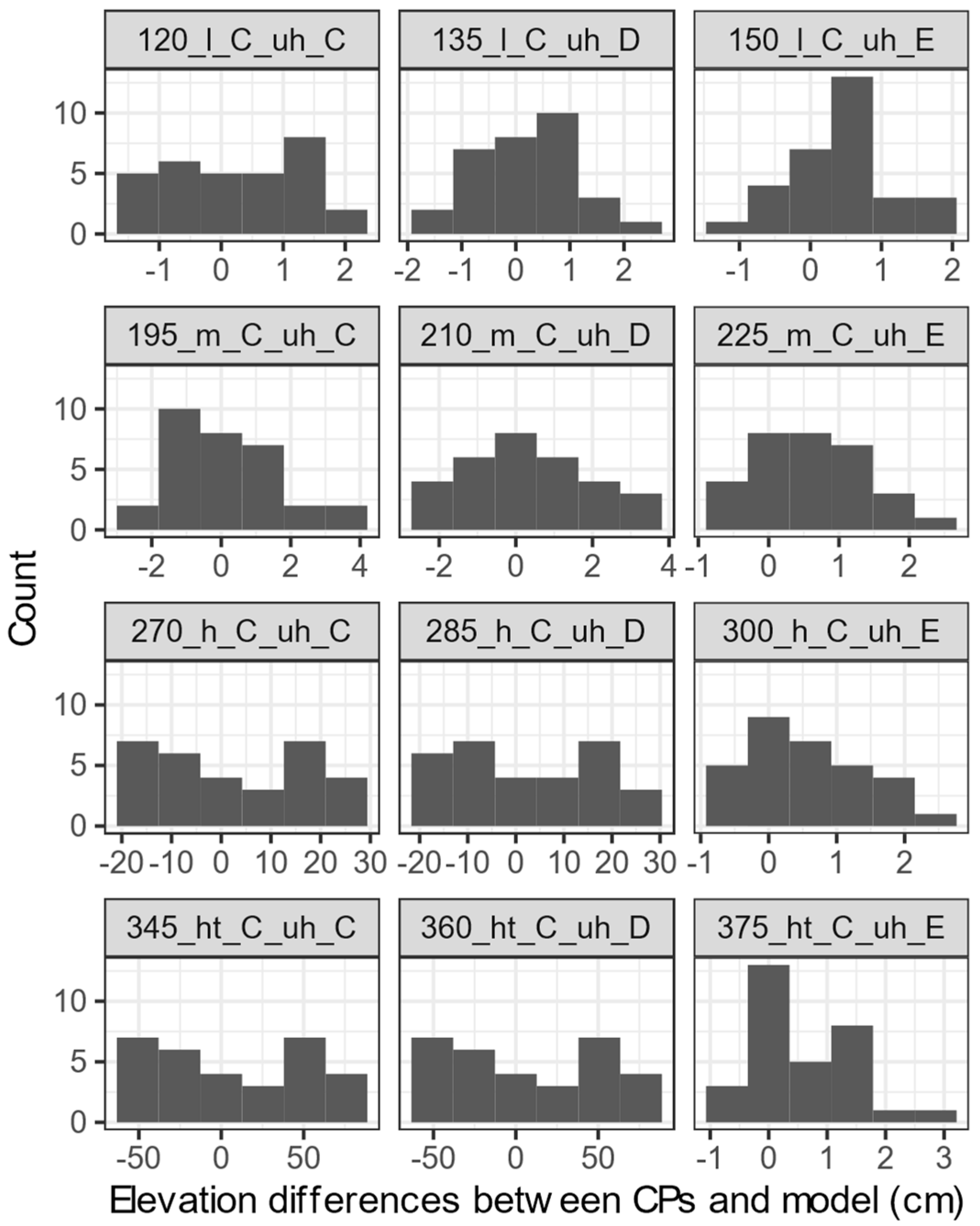
The levels of accuracy mentioned above determine the sampling rates at which the software processes the data. When the calculation accuracy is set to high at the image alignment stage, the software works on images with their original resolution. On the other hand, when the medium accuracy is set, the original image is reduced four times, in the low setting 16 times and in the lowest setting 64 times. For detailed photos, the highest level can be used, where the original resolution of the image is upscaled by a factor of 4 to find more key points. The meaning of these levels of settings is the same for the dense point cloud generation. In addition, during the image alignment step, the software calculates the optimization parameters that can be used to optimize the sparse point cloud. The f parameter is the focal length; cx and cy are intercepting axis of the lens optical with sensor plane; b1 and b2 are coefficients of affinity transformation and skew; coefficients k1, k2, k3 and k4 relate to radial distortion, and coefficients p1 and p2 to tangential distortion [63]. A detailed description of the processing steps, including the characteristics of the accuracy and quality settings, and a description of the optimization parameters process, can be found in the Agisoft Metashape software manual, available on the manufacturer’s website (https://www.agisoft.com/downloads/user-manuals/ accessed on 3 March 2022).
Taking into account all possible values of the above-mentioned parameters, 375 (5 × 3 × 5 × 5 = 375) different workflows were formulated and processed. In the first stage, an “initial” project was created in Agisoft Metashape to which the images and GCPs were imported in the UTM zone 28N coordinate system (EPSG: 25828). DNG photos were not modified or converted in any way before importing them into the software. Subsequently, GCPs were marked into all images. Prepared in this way, the project was duplicated 375 times in order to start processing in the next step in accordance with the adopted workflow for a given project. As part of the calculations, each sparse point cloud was filtered with the Gradual Selection tool, using the same parameters for all models (reprojection error = 0.5, reconstruction uncertainty = 10, image count = 2, projection accuracy = 20). The end result of the processing was a report, a DEM, and an orthomosaic (Figure 4).
In the next stage, DEMs were checked for height accuracy in the ArcMap software, using 30 CPs not participating in georeferencing. By selecting the Extract Values to Points tool, the differences in height between the CPs and the DEMs were obtained, and then the standard deviation and the root mean square error (RMSE) were calculated for the CPs of each model. We tested the accuracy of DEMs, not raw point clouds, as in most previous geomorphological works, DEMs were the most commonly used as final products for landform interpretation, mapping and change detection analysis [37]. In addition, we also visually checked raw point clouds in CloudCompare. For projects where RMSE values were low, the locations of control points were near to point cloud. For projects where RMSE values were high, control points were noticeably above or under the cloud. Additionally, based on the data from the report, the calculation time for each processing step was checked and the total calculation time for each project was summarized. Detailed information on each workflow is included in the Supplementary Materials (S1).

3. Results

Out of 375 projects, 195 did not generate a dense point cloud nor produced a DEM and orthomosaic. The step of aligning images at the lowest accuracy is responsible for the first 75 unsuccessful projects—the number of points remaining after filtration of sparse point clouds at this level (~600 points for all 75 chunks) was insufficient. Hence, the first result of the analysis is the statement that the level of accuracy of alignment set to lowest and subsequently filtered is insufficient to generate photogrammetric products. The sets of the “A” and “B” optimization parameters and alignment of images at low, medium, high, and highest accuracy are responsible for the remaining 120 projects, for which it was not possible to generate dense clouds. In these workflows, the sparse point clouds were not optimized with the k1 and k2 parameters, which were characterized by a high RMSE for GCPs of ~48.23 cm and a high reprojection error in the range of 2.74–5.80 pixels. Parameters k1 and k2 are responsible for the optimization of the sparse point cloud in terms of the radial distortion of the lens—the conclusion is that images from the DJI FC6310 camera are burdened with high radial distortion. Due to the absence of dense point clouds and DEMs in these projects, they were not included in any further work, and so only reports were generated.
In the remaining 180 projects, DEMs, orthomosaics and calculation reports were generated, in line with the planned workflows. The spatial resolution of the photogrammetric products depended on the level of accuracy set for dense point cloud generation—at the lowest level the resolution was ~28 cm, at the low level ~14 cm, at the medium level ~7 cm, at the high level ~3.5 cm, and at the ultra-high level ~1.75 cm. The spatial resolution of all orthomosaics was the same: 1.75 cm. RMSE and standard deviation based on CPs were calculated. From the obtained results, it can be concluded that when the accuracy of alignment of images was set to the high or highest level and then combined with the exclusion of k3, k4, p1, and p2 optimization parameters, the results were characterized by an increase in the RMSE value and standard deviation based on CPs. RMSE/SD for the high level reached the values of 14–15 cm, and for highest level 43–44 cm. The increase in the RMSE value and standard deviation based on CPs occurs with an increase in the number of points in the sparse cloud. Only when the optimization of the sparse point cloud was conducted using the set ”E” (optimization of the parameters f, cx, cy, k1, k2, k3, k4, p1, p2, b1, b2) were the high values of RMSE and standard deviations based on CPs reduced to values <2.5 cm. Figure 5 shows histograms for the 12 selected models, demonstrating the effect of parameters k3, k4, p1, and p2 on the height difference distribution based on CPs. Histograms of the height difference distribution, calculated based on CPs for each model, are included in S2 as Supplementary Materials. Moreover, a noticeable effect on the RMSE and standard deviation value was noted for the step of dense point cloud generation—with the increase in its quality and optimization of all parameters (set “E”), the values decrease.
In addition to analyzing the quality of the models, the calculation time for each step was checked, while calculation time for each project was summarized to compare the workflows in terms of calculation time and test if the increase in accuracy can be achieved with reasonable computing time. The step of generating a dense point cloud turned out to be crucial—the calculation time at the lowest level of accuracy may be shorter than ultra-high even six times, and between high and ultra-high three times (Table 1). The detailed results of the calculations, along with the quantitative and qualitative characteristics of the models, can be found in the Supplementary Materials (S1).

4. Discussion

In the following subsections, we discuss the impact of subsequent processing steps in SfM software on the accuracy of DEMs and orthomosaics.

4.1. Influence of Processing Parameters

4.1.1. Alignment of Images

The level of accuracy in the alignment of images may affect the results of standard deviations and RMSE based on CPs; nevertheless, for each level of accuracy in this step, values below 1 cm are possible to achieve. However, higher values in the order of 9, 15 or 44 cm were recorded where the level of accuracy was set to high or highest, the sparse point cloud was not optimized with the k3, k4, p1, and p2 parameters (“E” optimization parameter set), and no point limits were introduced in the sparse cloud. Such high results did not occur at the low and medium levels in projects with a similar number of points in a sparse cloud, hence the influence of the size of the sparse point cloud on this issue should be excluded. In addition, this step significantly influenced the calculation time—the use of high or highest level of accuracy, while not applying the key and tie points’ limits, only increased the calculation time, but did not increase the accuracy of the photogrammetric products. At the low and medium level of accuracy, the difference in calculation time was visibly lower. It has to be noted that downsampling of the original images (i.e., levels lowest, low, and medium) can mix spectral values of pixels. Therefore, in the case of large spectral differences between control points and surroundings, this aspect can influence the accuracy assessment.

4.1.2. Key and Tie Points’ Limits

The limit of key and tie points, with one exception, did not affect the accuracy of DEMs. In the group of projects with the set “A” (i.e., limit 10,000 key points and 1000 tie points), the lowest standard deviation based on CPs was 0.63 cm (which is the best result among all 180 projects). The most accurate project with the “B” set (i.e., limit 100,000 key points and 10,000 tie points) had a standard deviation of 0.65 cm, and with the “C” set (i.e., no limit on key or tie points) the standard deviation was 0.67 cm. Similar results of the sets “A”, “B” and “C” were also recorded for the RMSE values (0.76, 0.76, and 0.80 cm, respectively). The exception here is the generation of a sparse point cloud at the high and highest level of accuracy, plus a lack of optimization with parameters k3, k4, p1, and p2, which significantly reduces the accuracy of the models (standard deviation and RMSE based on CPs in the range of 9–44 cm). Such large values for high and highest settings can be potentially related to the general roughness of the surface or false matches related to similar texture of the studied area.
Therefore, increasing the number of points in the sparse cloud by increasing the limit of key and tie points or removing them completely does not always improve the accuracy of the models, and may result in an extension of the calculation time during its generation and subsequent processing steps. This applies, for example, to the three projects with the longest calculation times, of which the longest was almost five hours.

4.1.3. Dense Point Cloud Generation

The process of generating a dense point cloud turned out to be a significant element in terms of the accuracy of the models. High and ultra-high quality in combination with optimization of the parameters from the “E” set produced the best results—the resultant DEMs were characterized by standard deviation and RMSE based on CPs ≤ 1 cm. That likely results from the texture of the surface (gravels)—in this case, more characteristic points can be identified in the images and used to construct point cloud. The increase of quality of the dense point cloud generation step, along with the use of the key and tie points’ limits from the “A” set, result in a significant decrease in the value of the standard deviation and RMSE based on CPs. It should be underlined that calculating dense cloud with the highest possible quality resulted in the extension of the calculation time: in the case of the ultra-high quality, even several times. This is because the ultra-high settings oversample the original images and, therefore, quadruple memory consumption.

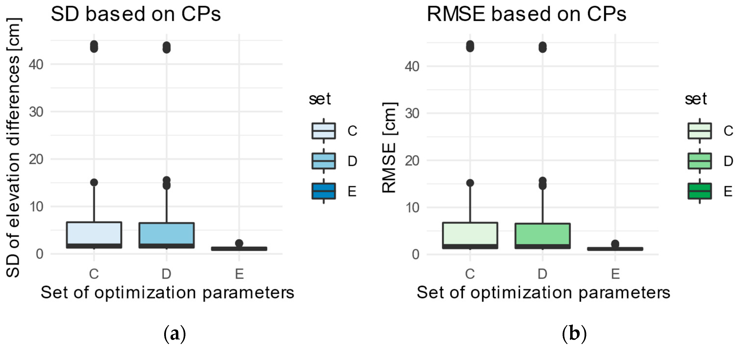
4.1.4. Optimization Alignment

The optimization of the sparse point cloud turned out to be the most important processing step in terms of the accuracy of DEMs. As mentioned in Section 3, projects with parameter sets “A” and “B” did not generate a dense point cloud. Only adding the parameters k1 and k2 to the sets “C”, “D”, and “E” resulted in the generation of a dense point cloud and photogrammetric products. These parameters relate to radial distortion [64], which characterizes the images from the DJI FC6310 camera [50], hence the lack of these parameters in the optimization could cause the problem with generation of a dense point cloud. The lowest RMSE and SD of CP errors were recorded in the workflows with the “E” set, in which all possible optimization parameters were applied, i.e., responsible for radial and tangential distortion, affinity and orthogonality. Nearly all the most accurate models in the experiment have been optimized with these parameters, therefore we recommend their use. A comparison of DEM accuracy results in relation to the optimization sets is presented in Figure 6. However, the possibility of overparameterization should be taken into account [65], for it may result in a poorly modeled surface and that is not reflected in its actual shape. It should be emphasized that the option to skip this step completely or partially should be used only when the operator has more reliable calibration parameters than those estimated by the software (for example, when using cameras calibrated in laboratory conditions). The gain in time is negligible compared to the significant loss in accuracy. Before the use of DEMs for further analyses, we recommend checking them first with CPs.

4.2. Best Workflows

Out of 180 completed projects, three workflows were selected, corresponding to the requirements formulated on account of the research aims. The main determinant was the low values of standard deviation and RMSE based on CPs in relation to the processing time of the set of images. On the other hand, when choosing the fastest procedure, it was assumed that the spatial resolution of the obtained DEM was better than 10 cm. The full characteristics of the workflows are presented in Table 2 based on the data contained in Supplementary Materials (S1).

4.3. Workflows in Python Scripts

In order to process many sets of images more efficiently or develop accurate DEMs and orthomosaics, workflows and their settings presented in the previous subsection were prepared in the form of Python scripts for Agisoft Metashape Professional (runs stable in version 1.7.1 build 11,797). The scripts are text files that run in the software with the Run script tool. They are written to make calculations on all chunks in an open project. The scripts should be used for projects with imported images, and to obtain a high-accuracy model, one should put GCPs on the images before running the scripts. Some of the previous studies have paid attention to the reproducibility of algorithms in Agisoft Metashape software, indicating that they may result in different outcomes (elevation variations ≥10 cm) even while using the same set of images and processed with exactly the same processing workflow [66]. For this reason, the scripts were checked on the same set of images used in the study, in which no significant differences were found based on reports and analysis of the results. Nevertheless, random differences in other larger sets of images cannot be excluded, such that the variance of the point cloud [50] or precision map [67] should be investigated before proceeding with further analysis of the processed data. The scripts are provided as Supplementary Materials for this article.

4.4. Potential Applications

The scripts can be used in the analysis of many research objects. The set of images analyzed in this study concerned proglacial areas with different terrain heights. Other potential applications may include, for instance, studies of alluvial fans [68], glacial landforms [40,69], glacier lake outburst floods [70,71] or aeolian landforms [72,73,74]. Furthermore, the scripts can be used for modelling various small objects, e.g., in archaeology [75] or geomorphology [76]. The presented scripts enabled a quick launch and systematic work, thereby making it possible to process more efficiently, e.g., several dozen large sets of images in agriculture [77], where each field can be used as a separate point of interest. The use of scripts, instead of selecting parameters manually, will be particularly helpful when processing many projects simultaneously in a computing cluster, positively influencing usage efficiency. This utility will be of most effective importance for multiannual, cyclical analyses of the same research areas (e.g., glaciers) [44,45], as it provides a constant, comparable workflow, reduces the time spent on calculations and project preparation, and will make comparisons between models more reliable, e.g., in research geomorphological fields such as change detection (e.g., [78]). In addition, field work may require a quick check on a portable notebook to ensure that the selected flight parameters (altitude, forward and side overlap of images) are sufficient to generate an accurate model. Script #1, with the shortest calculation time, may well be the answer to such needs. To increase the chance of repeating our results, we emphasize the importance of the quality of the input data and recommend the use of RAW images.

5. Conclusions

In this study, we delivered the first empirical test of the impact of processing parameters in Agisoft Metashape on the accuracy of the results of SfM processing based on typical application in geomorphological research. To achieve accurate DEM, it is crucial to use correct settings, including parameters optimizing a sparse point cloud. Moreover, needlessly increasing the level of accuracy of calculations does not always result in an increase in the accuracy of photogrammetric products, but may only extend the calculation process and delay the obtainment of results. To address these problems, three different workflows in the form of Python scripts for Agisoft Metashape were prepared, which, depending on the needs and available computing power, allow for the development of accurate models. For many scientists dealing with surface dynamics, scripts in which automating calculation work is performed should be a noticeable facilitation and may turn out to be a new method of improving quality in their research work. Key calculation settings and parameters, applied in the form of editable scripts, will increase the efficiency in processing and comparing large datasets, in addition to significant time savings due to the use of a powerful computing cluster. The high usability of the scripts is seen in the long-term observations, for example, of many glaciers and their forelands, where the automated workflow allows for a better management of numerous projects, not to mention rendering the process of comparing models reliable. Moreover, the authors do not exclude that the developed scripts will find their use in creating other three-dimensional models of various objects, not necessarily those related to glaciers and their forelands. In addition, it is suggested to perform the same experiment in the future for sets of images from several different cameras, and also including ground-based and oblique images.

Supplementary Materials

The following supporting information can be downloaded at: https://www.mdpi.com/article/10.3390/rs14061312/s1, S1: Detailed information on each workflow (Table S1), S2: Elevation differences between check points and model for each workflow, S3: Python Script #1 (the fastest), S4: Python Script #2 (optimal), S5: Python Script #3 (best quality).

Author Contributions

Conceptualization, S.Ś. and M.W.E.; methodology, S.Ś. and M.W.E.; software, S.Ś. and M.W.E.; validation, S.Ś. and M.W.E.; formal analysis, S.Ś.; investigation, S.Ś. and M.W.E.; resources, S.Ś. and M.W.E.; data curation, S.Ś.; writing—original draft preparation, S.Ś.; writing—review and editing, S.Ś. and M.W.E.; visualization, S.Ś.; supervision, M.W.E.; project administration, S.Ś. and M.W.E.; funding acquisition, M.W.E. All authors have read and agreed to the published version of the manuscript.

Funding

This research was funded by the National Science Centre, Poland, Grant Number 2019/35/B/ST10/03928.

Institutional Review Board Statement

Not applicable.

Informed Consent Statement

Not applicable.

Data Availability Statement

Data will be available on reasonable request.

Acknowledgments

This work would not be possible without the discussions and technical support from Adam Młynarczyk and Sławomir Królewicz.

Conflicts of Interest

The authors declare no conflict of interest. The funders had no role in the design of the study; in the collection, analyses, or interpretation of data; in the writing of the manuscript, or in the decision to publish the results.

References

  1. Ayalew, L.; Yamagishi, H. The application of GIS-based logistic regression for landslide susceptibility mapping in the Kakuda-Yahiko Mountains, Central Japan. Geomorphology 2005, 65, 15–31. [Google Scholar] [CrossRef]
  2. Stumvoll, M.J.; Schmaltz, E.M.; Glade, T. Dynamic characterization of a slow-moving landslide system—Assessing the challenges of small process scales utilizing multi-temporal TLS data. Geomorphology 2021, 389, 107803. [Google Scholar] [CrossRef]
  3. Turner, D.; Lucieer, A.; de Jong, S.M. Time Series Analysis of Landslide Dynamics Using an Unmanned Aerial Vehicle (UAV). Remote Sens. 2015, 7, 1736–1757. [Google Scholar] [CrossRef] [Green Version]
  4. Bourova, E.; Maldonado, E.; Leroy, J.-B.; Alouani, R.; Eckert, N.; Bonnefoy-Demongeot, M.; Deschatres, M. A new web-based system to improve the monitoring of snow avalanche hazard in France. Nat. Hazards Earth Syst. Sci. 2016, 16, 1205–1216. [Google Scholar] [CrossRef] [Green Version]
  5. Xiang, J.; Chen, J.; Sofia, G.; Tian, Y.; Tarolli, P. Open-pit mine geomorphic changes analysis using multi-temporal UAV survey. Environ. Earth Sci. 2018, 77, 220. [Google Scholar] [CrossRef]
  6. Kršák, B.; Blišťan, P.; Pauliková, A.; Puškárová, P.; Kovanič, Ľ.; Palková, J.; Zelizňaková, V. Use of low-cost UAV photogrammetry to analyze the accuracy of a digital elevation model in a case study. Measurement 2016, 91, 276–287. [Google Scholar] [CrossRef]
  7. Mohamed, I.N.L.; Verstraeten, G. Analyzing dune dynamics at the dune-field scale based on multi-temporal analysis of Landsat-TM images. Remote Sens. Environ. 2012, 119, 105–117. [Google Scholar] [CrossRef]
  8. Kociuba, W. Assessment of sediment sources throughout the proglacial area of a small Arctic catchment based on high-resolution digital elevation models. Geomorphology 2017, 287, 73–89. [Google Scholar] [CrossRef]
  9. Kociuba, W.; Kubisz, W.; Zagórski, P. Use of terrestrial laser scanning (TLS) for monitoring and modelling of geomorphic processes and phenomena at a small and medium spatial scale in Polar environment (Scott River—Spitsbergen). Geomorphology 2014, 212, 84–96. [Google Scholar] [CrossRef]
  10. Dietrich, J.T. Riverscape mapping with helicopter-based Structure-from-Motion photogrammetry. Geomorphology 2016, 252, 144–157. [Google Scholar] [CrossRef]
  11. Tomczyk, A.M.; Ewertowski, M.W.; Carrivick, J.L. Geomorphological impacts of a glacier lake outburst flood in the high arctic Zackenberg River, NE Greenland. J. Hydrol. 2020, 591, 125300. [Google Scholar] [CrossRef]
  12. Carrivick, J.L.; Smith, M.W. Fluvial and aquatic applications of Structure from Motion photogrammetry and unmanned aerial vehicle/drone technology. WIREs Water 2019, 6, e1328. [Google Scholar] [CrossRef] [Green Version]
  13. Ewertowski, M.W.; Tomczyk, A.M. Quantification of the ice-cored moraines’ short-term dynamics in the high-Arctic glaciers Ebbabreen and Ragnarbreen, Petuniabukta, Svalbard. Geomorphology 2015, 234, 211–227. [Google Scholar] [CrossRef] [Green Version]
  14. Tonkin, T.N.; Midgley, N.G.; Cook, S.J.; Graham, D.J. Ice-cored moraine degradation mapped and quantified using an unmanned aerial vehicle: A case study from a polythermal glacier in Svalbard. Geomorphology 2016, 258, 1–10. [Google Scholar] [CrossRef] [Green Version]
  15. Bernard, E.; Friedt, J.M.; Schiavone, S.; Tolle, F.; Griselin, M. Assessment of periglacial response to increased runoff: An Arctic hydrosystem bears witness. Land Degrad. Dev. 2018, 29, 3709–3720. [Google Scholar] [CrossRef] [Green Version]
  16. Sziło, J.; Bialik, R. Recession and Ice Surface Elevation Changes of Baranowski Glacier and Its Impact on Proglacial Relief (King George Island, West Antarctica). Geosciences 2018, 8, 355. [Google Scholar] [CrossRef] [Green Version]
  17. Carrivick, J.L.; Heckmann, T. Short-term geomorphological evolution of proglacial systems. Geomorphology 2017, 287, 3–28. [Google Scholar] [CrossRef] [Green Version]
  18. Song, X.P.; Hansen, M.C.; Stehman, S.V.; Potapov, P.V.; Tyukavina, A.; Vermote, E.F.; Townshend, J.R. Global land change from 1982 to 2016. Nature 2018, 560, 639–643. [Google Scholar] [CrossRef]
  19. Ding, Y.; Mu, C.; Wu, T.; Hu, G.; Zou, D.; Wang, D.; Li, W.; Wu, X. Increasing cryospheric hazards in a warming climate. Earth-Sci. Rev. 2021, 213, 103500. [Google Scholar] [CrossRef]
  20. Knight, J.; Harrison, S. Evaluating the impacts of global warming on geomorphological systems. Ambio 2012, 41, 206–210. [Google Scholar] [CrossRef] [Green Version]
  21. Hugonnet, R.; McNabb, R.; Berthier, E.; Menounos, B.; Nuth, C.; Girod, L.; Farinotti, D.; Huss, M.; Dussaillant, I.; Brun, F.; et al. Accelerated global glacier mass loss in the early twenty-first century. Nature 2021, 592, 726–731. [Google Scholar] [CrossRef] [PubMed]
  22. Dąbski, M.; Zmarz, A.; Rodzewicz, M.; Korczak-Abshire, M.; Karsznia, I.; Lach, K.; Rachlewicz, G.; Chwedorzewska, K. Mapping Glacier Forelands Based on UAV BVLOS Operation in Antarctica. Remote Sens. 2020, 12, 630. [Google Scholar] [CrossRef] [Green Version]
  23. Ewertowski, M.W.; Evans, D.J.A.; Roberts, D.H.; Tomczyk, A.M.; Ewertowski, W.; Pleksot, K. Quantification of historical landscape change on the foreland of a receding polythermal glacier, Hørbyebreen, Svalbard. Geomorphology 2019, 325, 40–54. [Google Scholar] [CrossRef] [Green Version]
  24. Benn, D.I.; Evans, D.J.A. Glaciers and Glaciation; Hodder Education: London, UK, 2010. [Google Scholar]
  25. Knight, J.; Harrison, S. Transience in cascading paraglacial systems. Land Degrad. Dev. 2018, 29, 1991–2001. [Google Scholar] [CrossRef]
  26. Knight, J.; Harrison, S. The impacts of climate change on terrestrial Earth surface systems. Nat. Clim. Chang. 2013, 3, 24–29. [Google Scholar] [CrossRef]
  27. Benn, D.I.; Bolch, T.; Hands, K.; Gulley, J.; Luckman, A.; Nicholson, L.I.; Quincey, D.; Thompson, S.; Toumi, R.; Wiseman, S. Response of debris-covered glaciers in the Mount Everest region to recent warming, and implications for outburst flood hazards. Earth-Sci. Rev. 2012, 114, 156–174. [Google Scholar] [CrossRef] [Green Version]
  28. Ewertowski, M.W.; Tomczyk, A.M. Reactivation of temporarily stabilized ice-cored moraines in front of polythermal glaciers: Gravitational mass movements as the most important geomorphological agents for the redistribution of sediments (a case study from Ebbabreen and Ragnarbreen, Svalbard). Geomorphology 2020, 350. [Google Scholar] [CrossRef]
  29. Carrivick, J.L.; Tweed, F.S. A review of glacier outburst floods in Iceland and Greenland with a megafloods perspective. Earth-Sci. Rev. 2019, 196, 102876. [Google Scholar] [CrossRef]
  30. Carrivick, J.L.; Tweed, F.S. A global assessment of the societal impacts of glacier outburst floods. Glob. Planet Chang. 2016, 144, 1–16. [Google Scholar] [CrossRef]
  31. Russell, A.J.; Carrivick, J.L.; Ingeman-Nielsen, T.; Yde, J.C.; Williams, M. A new cycle of jökulhlaups at Russell Glacier, Kangerlussuaq, West Greenland. J. Glaciol. 2011, 57, 238–246. [Google Scholar] [CrossRef] [Green Version]
  32. Colomina, I.; Molina, P. Unmanned aerial systems for photogrammetry and remote sensing: A review. ISPRS J. Photogramm. Remote Sens. 2014, 92, 79–97. [Google Scholar] [CrossRef] [Green Version]
  33. Smith, M.W.; Carrivick, J.L.; Quincey, D.J. Structure from motion photogrammetry in physical geography. Prog. Phys. Geogr. Earth Environ. 2016, 40, 247–275. [Google Scholar] [CrossRef] [Green Version]
  34. Carrivick, J.L.; Smith, M.W.; Quincey, D.J. Structure from Motion in the Geosciences; Wiley-Blackwell: Oxford, UK, 2016; p. 208. [Google Scholar]
  35. Anderson, K.; Gaston, K.J. Lightweight unmanned aerial vehicles will revolutionize spatial ecology. Front. Ecol. Environ. 2013, 11, 138–146. [Google Scholar] [CrossRef] [Green Version]
  36. Bhardwaj, A.; Sam, L.; Akanksha; Martín-Torres, F.J.; Kumar, R. UAVs as remote sensing platform in glaciology: Present applications and future prospects. Remote Sens. Environ. 2016, 175, 196–204. [Google Scholar] [CrossRef]
  37. Śledź, S.; Ewertowski, M.W.; Piekarczyk, J. Applications of unmanned aerial vehicle (UAV) surveys and Structure from Motion photogrammetry in glacial and periglacial geomorphology. Geomorphology 2021, 378, 107620. [Google Scholar] [CrossRef]
  38. Fugazza, D.; Scaioni, M.; Corti, M.; D’Agata, C.; Azzoni, R.S.; Cernuschi, M.; Smiraglia, C.; Diolaiuti, G.A. Combination of UAV and terrestrial photogrammetry to assess rapid glacier evolution and map glacier hazards. Nat. Hazards Earth Syst. Sci. 2018, 18, 1055–1071. [Google Scholar] [CrossRef] [Green Version]
  39. Westoby, M.J.; Brasington, J.; Glasser, N.F.; Hambrey, M.J.; Reynolds, J.M. ‘Structure-from-Motion’ photogrammetry: A low-cost, effective tool for geoscience applications. Geomorphology 2012, 179, 300–314. [Google Scholar] [CrossRef] [Green Version]
  40. Allaart, L.; Friis, N.; Ingólfsson, Ó.; Håkansson, L.; Noormets, R.; Farnsworth, W.R.; Mertes, J.; Schomacker, A. Drumlins in the Nordenskiöldbreen forefield, Svalbard. Gff 2018, 140, 170–188. [Google Scholar] [CrossRef]
  41. Storrar, R.D.; Ewertowski, M.; Tomczyk, A.M.; Barr, I.D.; Livingstone, S.J.; Ruffell, A.; Stoker, B.J.; Evans, D.J.A. Equifinality and preservation potential of complex eskers. Boreas 2019, 49, 211–231. [Google Scholar] [CrossRef] [Green Version]
  42. Tomczyk, A.M.; Ewertowski, M.W. UAV-based remote sensing of immediate changes in geomorphology following a glacial lake outburst flood at the Zackenberg river, northeast Greenland. J. Maps 2020, 16, 86–100. [Google Scholar] [CrossRef] [Green Version]
  43. Whitehead, K.; Moorman, B.J.; Hugenholtz, C.H. Brief Communication: Low-cost, on-demand aerial photogrammetry for glaciological measurement. Cryosphere 2013, 7, 1879–1884. [Google Scholar] [CrossRef] [Green Version]
  44. Chandler, B.M.P.; Evans, D.J.A.; Chandler, S.J.P.; Ewertowski, M.W.; Lovell, H.; Roberts, D.H.; Schaefer, M.; Tomczyk, A.M. The glacial landsystem of Fjallsjökull, Iceland: Spatial and temporal evolution of process-form regimes at an active temperate glacier. Geomorphology 2020, 361, 107192. [Google Scholar] [CrossRef]
  45. Westoby, M.J.; Rounce, D.R.; Shaw, T.E.; Fyffe, C.L.; Moore, P.L.; Stewart, R.L.; Brock, B.W. Geomorphological evolution of a debris-covered glacier surface. Earth Surf. Process. Landf. 2020, 45, 3431–3448. [Google Scholar] [CrossRef]
  46. Chandler, B.M.P.; Chandler, S.J.P.; Evans, D.J.A.; Ewertowski, M.W.; Lovell, H.; Roberts, D.H.; Schaefer, M.; Tomczyk, A.M. Sub-annual moraine formation at an active temperate Icelandic glacier. Earth Surf. Process. Landf. 2020, 45, 1622–1643. [Google Scholar] [CrossRef] [Green Version]
  47. Westoby, M.J.; Dunning, S.A.; Woodward, J.; Hein, A.S.; Marrero, S.M.; Winter, K.; Sugden, D.E. Sedimentological characterization of Antarctic moraines using UAVs and Structure-from-Motion photogrammetry. J. Glaciol. 2015, 61, 1088–1102. [Google Scholar] [CrossRef] [Green Version]
  48. Ewertowski, M.W.; Tomczyk, A.M.; Evans, D.J.A.; Roberts, D.H.; Ewertowski, W. Operational Framework for Rapid, Very-high Resolution Mapping of Glacial Geomorphology Using Low-cost Unmanned Aerial Vehicles and Structure-from-Motion Approach. Remote Sens. 2019, 11, 65. [Google Scholar] [CrossRef] [Green Version]
  49. James, M.R.; Chandler, J.H.; Eltner, A.; Fraser, C.; Miller, P.E.; Mills, J.P.; Noble, T.; Robson, S.; Lane, S.N. Guidelines on the use of structure-from-motion photogrammetry in geomorphic research. Earth Surf. Process. Landf. 2019, 44, 2081–2084. [Google Scholar] [CrossRef]
  50. James, M.R.; Antoniazza, G.; Robson, S.; Lane, S.N. Mitigating systematic error in topographic models for geomorphic change detection: Accuracy, precision and considerations beyond off-nadir imagery. Earth Surf. Process. Landf. 2020, 45, 2251–2271. [Google Scholar] [CrossRef]
  51. Gindraux, S.; Boesch, R.; Farinotti, D. Accuracy Assessment of Digital Surface Models from Unmanned Aerial Vehicles’ Imagery on Glaciers. Remote Sens. 2017, 9, 186. [Google Scholar] [CrossRef] [Green Version]
  52. Mesas-Carrascosa, F.-J.; Torres-Sánchez, J.; Clavero-Rumbao, I.; García-Ferrer, A.; Peña, J.-M.; Borra-Serrano, I.; López-Granados, F. Assessing Optimal Flight Parameters for Generating Accurate Multispectral Orthomosaicks by UAV to Support Site-Specific Crop Management. Remote Sens. 2015, 7, 12793–12814. [Google Scholar] [CrossRef] [Green Version]
  53. Sanz-Ablanedo, E.; Chandler, J.H.; Ballesteros-Pérez, P.; Rodríguez-Pérez, J.R. Reducing systematic dome errors in digital elevation models through better UAV flight design. Earth Surf. Processes Landf. 2020, 45, 2134–2147. [Google Scholar] [CrossRef]
  54. Sanz-Ablanedo, E.; Chandler, J.H.; Rodríguez-Pérez, J.R.; Ordóñez, C. Accuracy of Unmanned Aerial Vehicle (UAV) and SfM Photogrammetry Survey as a Function of the Number and Location of Ground Control Points Used. Remote Sens. 2018, 10, 1606. [Google Scholar] [CrossRef] [Green Version]
  55. Tonkin, T.; Midgley, N. Ground-Control Networks for Image Based Surface Reconstruction: An Investigation of Optimum Survey Designs Using UAV Derived Imagery and Structure-from-Motion Photogrammetry. Remote Sens. 2016, 8, 786. [Google Scholar] [CrossRef] [Green Version]
  56. Rangel, J.M.G.; Gonçalves, G.R.; Pérez, J.A. The impact of number and spatial distribution of GCPs on the positional accuracy of geospatial products derived from low-cost UASs. Int. J. Remote Sens. 2018, 39, 7154–7171. [Google Scholar] [CrossRef]
  57. Martínez-Carricondo, P.; Agüera-Vega, F.; Carvajal-Ramírez, F.; Mesas-Carrascosa, F.-J.; García-Ferrer, A.; Pérez-Porras, F.-J. Assessment of UAV-photogrammetric mapping accuracy based on variation of ground control points. Int. J. Appl. Earth Obs. Geoinf. 2018, 72, 1–10. [Google Scholar] [CrossRef]
  58. Cook, K.L.; Dietze, M. Short communication: A simple workflow for robust low-cost UAV-derived change detection without ground control points. Earth Surf. Dyn. 2019, 7, 1009–1017. [Google Scholar] [CrossRef] [Green Version]
  59. De Haas, T.; Nijland, W.; McArdell, B.W.; Kalthof, M.W.M.L. Case Report: Optimization of Topographic Change Detection with UAV Structure-From-Motion Photogrammetry Through Survey Co-Alignment. Front. Remote Sens. 2021, 2. [Google Scholar] [CrossRef]
  60. Forsmoo, J.; Anderson, K.; Macleod, C.J.A.; Wilkinson, M.E.; DeBell, L.; Brazier, R.E. Structure from motion photogrammetry in ecology: Does the choice of software matter? Ecol. Evol. 2019, 9, 12964–12979. [Google Scholar] [CrossRef]
  61. Nesbit, P.; Hugenholtz, C. Enhancing UAV–SfM 3D Model Accuracy in High-Relief Landscapes by Incorporating Oblique Images. Remote Sens. 2019, 11, 239. [Google Scholar] [CrossRef] [Green Version]
  62. Peppa, M.V.; Hall, J.; Goodyear, J.; Mills, J.P. Photogrammetric Assessment and Comparison of Dji Phantom 4 Pro and Phantom 4 Rtk Small Unmanned Aircraft Systems. Int. Arch. Photogramm. Remote Sens. Spat. Inf. Sci. 2019, XLII-2/W13, 503–509. [Google Scholar] [CrossRef] [Green Version]
  63. Agisoft. Agisoft Metashape User Manual Professional Edition, Version 1.8; Agisoft LLC: St. Petersburg, Russia, 2022; p. 195. [Google Scholar]
  64. Carbonneau, P.E.; Dietrich, J.T. Cost-effective non-metric photogrammetry from consumer-grade sUAS: Implications for direct georeferencing of structure from motion photogrammetry. Earth Surf. Process. Landf. 2017, 42, 473–486. [Google Scholar] [CrossRef] [Green Version]
  65. James, M.R.; Robson, S.; d’Oleire-Oltmanns, S.; Niethammer, U. Optimising UAV topographic surveys processed with structure-from-motion: Ground control quality, quantity and bundle adjustment. Geomorphology 2017, 280, 51–66. [Google Scholar] [CrossRef] [Green Version]
  66. Hendrickx, H.; Vivero, S.; De Cock, L.; De Wit, B.; De Maeyer, P.; Lambiel, C.; Delaloye, R.; Nyssen, J.; Frankl, A. The reproducibility of SfM algorithms to produce detailed Digital Surface Models: The example of PhotoScan applied to a high-alpine rock glacier. Remote Sens. Lett. 2018, 10, 11–20. [Google Scholar] [CrossRef] [Green Version]
  67. James, M.R.; Robson, S.; Smith, M.W. 3-D uncertainty-based topographic change detection with structure-from-motion photogrammetry: Precision maps for ground control and directly georeferenced surveys. Earth Surf. Process. Landf. 2017, 42, 1769–1788. [Google Scholar] [CrossRef]
  68. Tomczyk, A.M.; Ewertowski, M.W.; Stawska, M.; Rachlewicz, G. Detailed alluvial fan geomorphology in a high-arctic periglacial environment, Svalbard: Application of unmanned aerial vehicle (UAV) surveys. J. Maps 2019, 15, 460–473. [Google Scholar] [CrossRef] [Green Version]
  69. Ely, J.C.; Graham, C.; Barr, I.D.; Rea, B.R.; Spagnolo, M.; Evans, J. Using UAV acquired photography and structure from motion techniques for studying glacier landforms: Application to the glacial flutes at Isfallsglaciären. Earth Surf. Process. Landf. 2017, 42, 877–888. [Google Scholar] [CrossRef]
  70. Wilson, R.; Harrison, S.; Reynolds, J.; Hubbard, A.; Glasser, N.F.; Wündrich, O.; Iribarren Anacona, P.; Mao, L.; Shannon, S. The 2015 Chileno Valley glacial lake outburst flood, Patagonia. Geomorphology 2019, 332, 51–65. [Google Scholar] [CrossRef]
  71. Tomczyk, A.M.; Ewertowski, M.W. Baseline data for monitoring geomorphological effects of glacier lake outburst flood: A very-high-resolution image and GIS datasets of the distal part of the Zackenberg River, northeast Greenland. Earth Syst. Sci. Data 2021, 13, 5293–5309. [Google Scholar] [CrossRef]
  72. Mancini, F.; Dubbini, M.; Gattelli, M.; Stecchi, F.; Fabbri, S.; Gabbianelli, G. Using Unmanned Aerial Vehicles (UAV) for High-Resolution Reconstruction of Topography: The Structure from Motion Approach on Coastal Environments. Remote Sens. 2013, 5, 6880–6898. [Google Scholar] [CrossRef] [Green Version]
  73. Van Puijenbroek, M.E.B.; Nolet, C.; de Groot, A.V.; Suomalainen, J.M.; Riksen, M.J.P.M.; Berendse, F.; Limpens, J. Exploring the contributions of vegetation and dune size to early dune development using unmanned aerial vehicle (UAV) imaging. Biogeosciences 2017, 14, 5533–5549. [Google Scholar] [CrossRef] [Green Version]
  74. Solazzo, D.; Sankey, J.B.; Sankey, T.T.; Munson, S.M. Mapping and measuring aeolian sand dunes with photogrammetry and LiDAR from unmanned aerial vehicles (UAV) and multispectral satellite imagery on the Paria Plateau, AZ, USA. Geomorphology 2018, 319, 174–185. [Google Scholar] [CrossRef]
  75. Lauria, G.; Sineo, L.; Ficarra, S. A detailed method for creating digital 3D models of human crania: An example of close-range photogrammetry based on the use of Structure-from-Motion (SfM) in virtual anthropology. Archaeol. Anthropol. Sci. 2022, 14. [Google Scholar] [CrossRef]
  76. Eichel, J.; Draebing, D.; Kattenborn, T.; Senn, J.A.; Klingbeil, L.; Wieland, M.; Heinz, E. Unmanned aerial vehicle-based mapping of turf-banked solifluction lobe movement and its relation to material, geomorphometric, thermal and vegetation properties. Permafr. Periglac. Processes 2020, 31, 97–109. [Google Scholar] [CrossRef]
  77. Zhang, C.; Kovacs, J.M. The application of small unmanned aerial systems for precision agriculture: A review. Precis. Agric. 2012, 13, 693–712. [Google Scholar] [CrossRef]
  78. Midgley, N.G.; Tonkin, T.N.; Graham, D.J.; Cook, S.J. Evolution of high-Arctic glacial landforms during deglaciation. Geomorphology 2018, 311, 63–75. [Google Scholar] [CrossRef]
Figure 1. Location of the study area and a photo from the study area where the flight took place. The study areas represent a typical proglacial landscape, built from sands and gravel.
Remotesensing 14 01312 g001
Figure 2. (a) Example of an established GCP; (b) method of measuring points with the GNSS receiver. GNSS measurement was carried out on the middle stone in the circle, which differed from the others by its size and shape.
Remotesensing 14 01312 g002
Figure 3. Scheme of project’s code naming.
Remotesensing 14 01312 g003
Figure 4. Example of end results of the processing: a DEM and an orthomosaic, with locations of GCPs and CPs.
Remotesensing 14 01312 g004
Figure 5. Distribution of the difference in elevation between 30 CPs and DEMs for the 12 selected workflows. The histograms are arranged according to the sets of optimization parameters and the level of accuracy of image alignment: in the first column there are four histograms for projects with the “C” set, in the second with the “D” set, and in the third with the “E” set. The level of accuracy for generating the sparse point cloud in the column is set from low (first row) to highest (fourth row). All histograms are for projects where the quality of dense point cloud generation has been set to ultra-high. The following regularities can be seen: (1) increasing the quality of generating a sparse point cloud increases the differences in elevation for models with optimized parameter sets “C” and “D” (approximately from −2 to 2 cm for low, from −2 to 4 cm for medium, from −20 to 30 cm for high and from −50 to 50 cm for ultra-high quality); (2) optimization of the sparse point cloud with all parameters (set “E”) significantly affects the accuracy of the models, resulting in the standard deviation of <2.5 cm.
Remotesensing 14 01312 g005
Figure 6. Distribution of standard deviation (a) and RMSE (b) values based on CPs. The figure suggests that use of the “E” set would result in lower error values. For the projects with the “E” set, no DEMs with very high errors of ~45 cm were found.
Remotesensing 14 01312 g006
Table 1. An example of the calculation time data from Supplementary Materials (S1) for each processing step. The data concern 15 projects which include: accuracy of alignment of images at the medium level, three different sets of tie points and key point limits, accuracy of generating a dense cloud of points at five different levels, and a set “C” of optimization parameters. It is clearly visible that the step of generating a dense point cloud is the most time consuming. It is worth noting that the orthomosaic generation step can account for over 60% of the calculation time (e.g., project 181_m_A_lt_C).
Project’s CodeCalculation Time (h)
Alignment of ImagesOptimization ParametersDense Point Cloud GenerationDEM
Generation
Orthomosaic
Generation
SUM
181_m_A_lt_C00:03:4700:00:0000:07:4400:00:0600:19:1900:30:56
182_m_B_lt_C00:04:3000:00:0500:07:0900:00:0500:20:2800:32:17
183_m_C_lt_C00:05:1300:00:0400:06:2300:00:0500:21:2200:33:07
184_m_A_l_C00:03:4500:00:0100:07:1800:00:1200:21:1200:32:28
185_m_B_l_C00:04:4900:00:0600:07:0900:00:1100:21:0200:33:17
186_m_C_l_C00:05:0300:00:0400:07:0100:00:1000:20:5600:33:14
187_m_A_m_C00:03:5300:00:0100:23:1500:00:4500:19:3300:47:27
188_m_B_m_C00:04:5300:00:0400:14:4800:00:3600:19:4800:40:09
189_m_C_m_C00:05:0400:00:0800:13:2900:00:3300:19:5200:39:06
190_m_A_h_C00:03:4900:00:0100:47:0100:02:0700:20:0001:12:58
191_m_B_h_C00:04:5400:00:0300:46:0900:01:5600:19:3301:12:35
192_m_C_h_C00:05:0400:00:0700:48:0800:02:0000:19:0501:14:24
193_m_A_uh_C00:03:5000:00:0102:51:0000:06:3300:25:2003:26:44
194_m_B_uh_C00:05:0000:00:0402:34:0000:06:1100:24:1903:09:34
195_m_C_uh_C00:04:3800:00:0602:44:0000:07:0400:23:0003:18:48
Table 2. Detailed description of the three workflows that meet the requirements formulated in view of the research aims. The difference in the SD of CP errors between workflows I and II is 0.38 cm, and between II and III only 0.07 cm. However, the workflows differ from each other mainly in terms of the time of calculations, which in the I type was more than seven times faster than the III type. The conclusion is that setting higher levels of accuracy in the software is not always appropriate (remembering that the total calculation time depends mainly on the computing power).
Type
of Workflow
Project’s CodeProcessing ParametersDEM
GSD
(cm)
RMSE
(cm)
SD of
Elevation
Differences
(cm)
Calculation
Time
(h)
I. The fastest128_l_B_m_D1. Alignment accuracy: low.
2. Count of key and tie points: 100,000 (key points),
10,000 (tie points).
3. Dense point cloud generation quality: medium.
4. Optimization parameters: f, cx, cy, k1, k2, b1, b2.
7.011.031.0100:35:08
II. Optimal147_l_C_h_E1. Alignment accuracy: low.
2. Count of key and tie points: no limits.
3. Dense point cloud generation quality: high.
4. Optimization parameters: f, cx, cy, k1, k2, k3, k4,
p1, p2, b1, b2.
3.500.810.7001:05:14
III. Best quality223_m_A_uh_E1. Alignment accuracy: medium
2. Count of key and tie points: 10,000 (key points),
1000 (tie points).
3. Dense point cloud generation quality: ultra-high.
4. Optimization parameters: f, cx, cy, k1, k2, k3, k4,
p1, p2, b1, b2.
1.750.760.6303:47:02
Publisher’s Note: MDPI stays neutral with regard to jurisdictional claims in published maps and institutional affiliations.

