Development of a Multi-Index Method Based on Landsat Reflectance Data to Map Open Water in a Complex Environment

Abstract

Mapping surface water extent is important for managing water supply for agriculture and the environment. Remote sensing technologies, such as Landsat, provide an affordable means of capturing surface water extent with reasonable spatial and temporal coverage suited to this purpose. Many methods are available for mapping surface water including the modified Normalised Difference Water Index (mNDWI), Fisher’s water index (FWI), Water Observations from Space (WOfS), and the Tasseled Cap Wetness index (TCW). While these methods can discriminate water, they have their strengths and weaknesses, and perform at their best in different environments, and with different threshold values. This study combines the strengths of these indices by developing rules that applies an index to the environment where they perform best. It compares these indices across the Murray-Darling Basin (MDB) in southeast Australia, to assess performance and compile a heuristic rule set for accurate application across the MDB. The results found that all single indices perform well with the Kappa statistic showing strong agreement, ranging from 0.78 for WOfS to 0.84 for TCW (with threshold −0.035), with improvement in the overall output when the index best suited for an environment was selected. mNDWI (using a threshold of −0.3) works well within river channels, while TCW (with threshold −0.035) is best for wetlands and flooded vegetation. FWI and mNDWI (with threshold 0.63 and 0, respectively) work well for remaining areas. Selecting the appropriate index for an environment increases the overall Kappa statistic to 0.88 with a water pixel accuracy of 90.5% and a dry pixel accuracy of 94.8%. An independent assessment illustrates the benefit of using the multi-index approach, making it suitable for regional-scale multi-temporal analysis.

1. Introduction

Surface water is vital for human consumption, agricultural use, as well as maintaining the environmental health of wetlands and rivers [1]. Mapping surface water extent is an important step in estimating water volume, and monitoring these changes is necessary as a growing population and changing climate are leading to increased pressure on water supply [2]. This reduction in water leads to stress on water environments, such as wetlands, floodplains and billabongs, and their connectivity to the river systems [3], meaning accurate information on available water is vital. This is particularly true in much of Australia, which is becoming hotter and dryer in recent times [4]. In addition, mapping surface water extent is essential for identifying flood-affected areas to support flood risk assessment, emergency response service, property valuation, insurance cost estimation, sediment/contaminant transport, infrastructure planning, hydraulic engineering, and so on [5,6,7].

Ground observations of surface water extent can provide valuable information, but are not always available, especially during flood events when field instruments may be destroyed, and sampling can be dangerous. It is also hard to obtain large scale synopsis of current and historical water extent through gauging stations and high-water marks; furthermore, rating curves are not always reliable [8,9]. Remote sensing technologies provide an affordable means of capturing surface water extent with reasonable spatial and temporal coverage suited to the purpose of water monitoring [10]. The spatial resolution of the Landsat satellite series (30 m) [11] makes it suitable for capturing much of the fine hydro morphological features of a large river basin, at a temporal scale of 8–16 days (depending on the number of operating sensors and effects of cloud cover). It also has a rich archive of data dating back to 1987 for the thematic mapper series [11]. The European Space Agency’s Sentinel-2 sensors provide a finer spatial resolution (10–20 m), and more frequent observations (5–10 days); however, the data only became available from 2015, with more regular coverage after the second sensor (Sentinel-2b) was launched in 2017 [12]. Sentinel-2 also has applications in mapping surface water [13,14,15].

There are many methods available for mapping surface water using surface reflectance from remote sensing data [16,17,18] including the Landsat series [19,20,21,22]. Some of the more complex methods use machine learning or other classification techniques [23,24,25,26,27]. Spectral indices are typically used for mapping surface water due to their simplicity and ease of application [28,29,30,31,32]. Some of the more commonly used, validated, and available methods within Australia are the modified Normalised Difference Water Index (mNDWI) [29], Geoscience Australia’s Water Observations from Space (WOfS; [7]), and a water index by Fisher et al. (2016) [31]. The mNDWI uses the green and shortwave infrared (SWIR-1) surface reflectance bands [29], while Fisher et al. [31] developed a new index suitable for mapping surface water with Landsat data across eastern Australia that uses the green, red, near infrared (NIR), SWIR-1, and SWIR-2 surface reflectance bands. The WOfS dataset is generated by Geoscience Australia and available through Digital Earth Australia [7]. WOfS uses a decision tree approach based on a selection of Landsat spectral bands and indices, as well as ancillary products (including topography and hydrology layers) to constrain water extent to likely areas. Individual WOfS images of surface water extent, along with summary statistics, are available for Australia for the whole Landsat archive (since 1987). These methods are designed to map open surface water, leaving flooded vegetation underestimated. To help overcome this gap, Geoscience Australia has invested time and effort into incorporating the Tasseled Cap Wetness index (TCW) [33] into a wetland mapping tool [34]. The TCW index uses the blue, green, red, NIR, SWIR-1, and SWIR-2 surface reflectance bands [33].

These indices have their strengths and weaknesses, as well as preferred thresholds for different applications depending on vegetation cover, soil colour, soil moisture, and water colour [31]. Variable thresholds of water indices have been adopted to help overcome this challenge [35,36,37,38]. While there is no single index or threshold that works for all applications [22], the mNDWI is often the preferred index in comparisons [36]. For mNDWI [29], pixels with values greater than zero are water, which also agrees with the work of Fisher et al. (2016) [31]. However, Sims et al. (2014) [39] found a threshold value of −0.3 for water was more successful at capturing water extent at a range of sites along the Murrumbidgee River in southeast Australia. This threshold (−0.3) has been subsequently used for mapping flooding and persistent waterholes in Northern Australia [40], as well as flood events in the Fitzroy River in Western Australia [41] and the northern Murray Darling Basin (MDB; [42]). However, it has been found to overestimate surface water extent along the dark floodplains in central Australia (the Cooper basin), and a threshold of zero was found to be more suitable [43]. A threshold value of −0.5 has been used to identify inundated vegetation [44], but constraints were required to reduce commission errors outside of these areas. Zhai et al. (2015) [45] found a positive threshold (0.2 to 0.31) worked best in an urban environment.

The WOfS data were designed to provide a conservative estimate of surface water extent, making it a robust product, but it is more likely to underestimate, rather than overestimate water extent [40]. Ticehurst et al. (2017) [46] found an mNDWI of −0.3 performed better than WOfS for a selection of flood events in the MDB. Geoscience Australia has utilised the Tasseled Cap Wetness index to map flooded vegetation as part of their Wetland Insite Tool [34] based on a TCW index threshold of −0.035, which can detect more water under flooded vegetation compared to other indices.

Fisher et al. (2016) [31] compared seven water index methods (including mNDWI and TCW), as well as their new water index, for a range of water and non-water plots. Their results showed that most indices performed well. Fisher’s water index (now referred to as FWI) performed best at correctly identifying pure water pixels with a threshold of 0.63, while for TCW the threshold was −0.01. While the investigation of Fisher et al. (2016) [31] was extensive in comparing Landsat-derived water indices over eastern Australia, it did not include WOfS data, or some of the thresholds mentioned earlier.

The aim of this study was to evaluate different methods of inundation mapping and identify the index that produces best results within different environments across the MDB. In particular, the goal is to develop a rule set to apply different indices in the environment where they perform best across the whole of the MDB for achieving the best estimate of surface water. This multi-index method needs to be relatively simple and fast to process across the whole basin. Another aim was to maximise the capture of small water bodies where possible, without compromising commission errors for water pixels. The MDB study sites, followed by an explanation of each index, as well as the data used for validating results across the MDB are described in Section 2. The results of the evaluation are provided in Section 3, including the new decision rule set to provide the most suitable water index across each environment. Section 4 discusses some of the issues and advantages in using the new multi-index method followed by the conclusion.

2. Materials and Methods

2.1. Study Site

The MDB, located in southeastern Australia (Figure 1), covers an area more than one million square kilometres, and contains a total of approximately 440,000 km of rivers, with 40,000 km of major rivers [47]. The MDB contains over 30,000 wetlands, with 16 of those being internationally significant (according to the Ramsar Convention [48]). It also produces around 40% of Australia’s agricultural output [49]. Land within the basin is used mainly for forestry, livestock grazing, dryland, and irrigated cropping [47] and is home to more than two million people [49]. The two major rivers in the MDB are the Darling River and the Murray River (shown as green and red respectively in Figure 1). The northern section of the MDB consists of mostly unregulated ephemeral rivers and streams, although major water storages exist along some of the rivers, while the southern section contains mostly regulated rivers with major water storages in many of them [47,50]. Water use in the basin has increased over time, which when combined with periods of drought, has led to the degradation of rivers and wetlands [51]. This means water monitoring and management within the basin is of particular importance.

2.2. Remote Sensing Data

All Landsat data were sourced from Digital Earth Australia (DEA; [52,53,54]) as analysis-ready Landsat surface reflectance from the Landsat 5 (Thematic Mapper), Landsat 7 (Enhanced Thematic Mapper), and Landsat 8 (Operational Land Imager) sensors. The MDB covers 62 individual Landsat path/row scenes; however, only the areas of interest used for testing and validation were required from DEA. WOfS water maps were also sourced through DEA for the same areas of interest and dates. Extraction of the data was performed using python code in Jupyter Notebooks (which is a web-based interactive computing platform), with a virtual desktop instance on the Australian National Computational Infrastructure (NCI) [55].

2.3. GIS Data

The Australia Hydrological Geospatial Fabric (Geofabric) and the Australian National Aquatic Ecosystem (ANAE) datasets were used for defining different water environments across the MDB.

The Geofabric (version 3) is a collection of hydrological spatial layers across Australia [56]. It was originally built to meet the Australian Bureau of Meteorology’s requirements for water accounting and assessment. The input data consist of topologically connected surface water hydrology, a Digital Elevation Model, streamlines, and catchment boundaries [56,57]. The data are provided at 1:100,000 scale.

The ANAE classification framework consists of a rule-based approach to surface and subterranean aquatic ecosystems [58]. This interim framework (version 2.0) was used to classify freshwater and estuarine aquatic ecosystems in the MDB. It used available data of the highest spatial resolution that best represented the aquatic ecosystems within the MDB [58,59]. The ANAE wetlands layer consists of Palustrine and Lacustrine systems of wetlands within the MDB, with artificial systems (such as dams and irrigation channels) removed where possible.

2.4. Validation Data

An extensive validation dataset is available from Fisher et al. (2016) [31] for eastern Australia. In total, 440 plots, of 300 m × 300 m in size, were used that fell within the MDB and where DEA Landsat data were available. These validation plots had been manually digitised from high-resolution airborne imagery as well as a small selection of Google Earth imagery [31]. The high-resolution airborne imagery was a three-band (blue, green, and red) Leica Airborne Digital Sensor at a 0.5 m spatial resolution, as well as some three-band (red, green, and NIR) imagery acquired during flood events to improve the identification of turbid water. The Google Earth images were true-colour images from Quickbird-2 at a 0.6 m spatial resolution. Water within each validation plot was classified by manually digitised polygons around each water body [31]. All validation plots and dates were matched to Landsat acquisitions, and captured all four seasons of the year. These sites included flood events, large storage dams and small water bodies, in-channel waterholes, as well as plots without water (steep topography, cloud shadow, quarries, and urban sites), making it a valuable dataset for validation. While these validation plots were collected at times that used different Landsat sensors, a comparison analysis on the influence of Landsat sensor (Landsat 5, 7, and 8) on index showed minimal difference [31]. The dates of image acquisition used to extract the validation plots coinciding with the Landsat sensors range from 2007 to 2013 (using both Landsat 5 and Landsat 7 images), and their extents can be seen in Figure 1.

Hydrodynamic (HD) modelling output along the Murray River was also used as validation of a flood event in September 2011, which coincided with a cloud-free Landsat scene [60]. The accuracy of the HD model output is estimated to be good in this area (zone 5) with comparison of simulated and observed water levels ranging from 0.94 to 0.98 R² [60]. This HD model output also overlapped with some ANAE wetland sites, including flooded vegetation. Twenty plots of same size as Fisher et al. (2016) [31] were generated from this scene, with 10 covering the river channel, and 10 including ANAE wetlands. In addition to this, an extra 11 plots of urban areas were included to further test for commission errors in the indices. These urban plots are the same size as the other validation plots and are located within the Landsat scenes of the Fisher et al. (2016) [31] validation sites (i.e., locations of the Landsat images and dates that contain the validation plots; Figure 1). This resulted in a total of 461 validation plots (or approximately 46,100 Landsat pixels), scattered throughout the MDB and included a variety of surface water characteristics.

2.5. Water Indices

In order to identify which water indices perform best across the different environments, the mNDWI, FWI, WOfS, and TCW were produced from the Landsat images for the validation sites and compared across the MDB for a range of large permanent water bodies, waterholes, river channels, wetlands, and floodplains. Based on past research [7,29,31,34,39], different thresholds were selected for the same index where appropriate, resulting in a total of six indices to test (

Table 1. Indices used for assessing mapping of surface water extent within the MDB. ‘Name’ is the name used to identify the index/threshold in remainder of this study. Bands correspond to Landsat satellites.

Water Index	Algorithm	Threshold	Name	References
modified Normalised Difference Water Index (mNDWI)	$\frac{\mathrm{green}-\mathrm{SWIR}1}{\mathrm{green}+\mathrm{SWIR}1}$	0.0	mNDWI0	[29,31]
		−0.3	mNDWInp3	[39]
Fisher’s Water Index (FWI)	$1.7204+171\times \mathrm{green}+3\times \mathrm{red}-70\times \mathrm{NIR}-45\times \mathrm{SWIR}1-71\times \mathrm{SWIR}2$	0.63	FWI	[31]
Water Observations from Space (WOfS)	(see footnote 1)	NA	WOfS	[7]
Tasseled Cap Wetness index (TCW)	$0.0315\times \mathrm{blue}+0.2021\times \mathrm{green}+0.3102\times \mathrm{red}+0.1594\times \mathrm{NIR}-0.6806\times \mathrm{SWIR}1-0.6109\times \mathrm{SWIR}2$	−0.01	TCWnp01	[31]
		−0.035	TCWnp035	[34]

¹ WOfS uses a decision tree approach based on a selection of Landsat spectral bands and indices, and includes ancillary products [7].

).

As reported in Fisher et al. (2016) [31], FWI and mNDWI (with a threshold of 0) perform better for different coloured water bodies. Hence, these indices were combined (i.e., maximum water extent of FWI and mNDWI) to maximise the chances of capturing surface water in smaller water bodies, accounting for the variation of water colour within the MDB. This maximum of FWI and mNDWI (referred to as Max_{fwi_ndwi}) is defined as:

$${\mathrm{Max}}_{\mathrm{fwi}\_\mathrm{ndwi}}=\left(\mathrm{mNDWI}>0.0\right)\vee (\mathrm{FWI}>0.63)$$

(1)

For Max_{fwi_ndwi}, a pixel is inundated if Equation (1) is true. Max_{fwi_ndwi} was also compared to the other indices. The estimated surface water area within each validation plot was also plotted against true surface water area to identify which indices performed best, including with respect to the smaller water bodies.

2.6. Topology of the Murray Darling Basin

As mentioned in Section 1, different indices and thresholds perform better depending on the vegetation cover, soil colour, soil moisture, and water colour. The MDB was separated into four basic environments, as they relate to water:

• Major Perennial Rivers (as defined within the Geofabric; [56]) with a 100 m buffer along the streamline;
• Australian National Aquatic Ecosystem (ANAE) Wetlands [58,59,61]. This includes all natural perennial and temporary lakes, billabongs, and floodplains, as well as many of the minor river channels;
• Large Water Storage (as defined within the Geofabric; [56]). Although it is defined as large water storage, this layer includes both small (~5 ha) and large artificial water reservoirs;
• Remaining area. This includes the remaining rivers and streams (those that are not already defined as major perennial rivers in the Geofabric, or within the ANAE Wetlands layer), small dams, agriculture and farming areas, native and plantation forests, areas with steep topography, and urban and other built-up areas.

These three main water environments (Major Perennial Rivers, Wetlands, and Large Water Storage) were selected, as they covered the entire MDB, were compatible with the level of detail at the Landsat spatial resolution, and they covered a large proportion of surface water visible in the Landsat imagery (Figure 1). These layers were later used in the accuracy assessment of water indices for the validation plots for: (i) all plots (which does not consider individual layers), (ii) major perennial rivers, (iii) wetlands, (iv) large water storage, (v) remaining area containing water, and (vi) remaining area without surface water.

2.7. Validation and Assessment

The producer’s accuracy [62] of water pixels (Equation (2)), dry pixels (Equation (3)), and the Kappa statistic (K) [63,64] (Equations (4) and (5)) was calculated for all the validation plots combined, as well as broken down into the four environment types (major perennial rivers, wetlands, large water storage, and remaining area with and without surface water):

$$\mathrm{PA}\_\mathrm{water}=100\ast \frac{\mathrm{number}\mathrm{correctly}\mathrm{classified}\mathrm{water}\mathrm{pixels}}{\mathrm{total}\mathrm{validation}\mathrm{water}\mathrm{pixels}}$$

(2)

$$\mathrm{PA}\_\mathrm{dry}=100\ast \frac{\mathrm{number}\mathrm{correctly}\mathrm{classified}\mathrm{dry}\mathrm{pixels}}{\mathrm{total}\mathrm{validation}\mathrm{dry}\mathrm{pixels}}$$

(3)

Kappa (K) estimates the agreement between two rasters, while also accounting for agreement occurring by chance. It is considered to be a robust but conservative measure of agreement:

$$\mathrm{K}=\left(s/n-Pc\right)/\left(1-Pc\right)$$

(4)

where s is the total number of correct pixels, n is the total number of pixels, and Pc is defined as follows:

$$Pc=\left(a1\times b1+a0\times b0\right)/\left(n\times n\right)$$

(5)

where a1 and b1 are the number of water pixels and a0 and b0 are the number of dry pixels in the Landsat and validation plots, respectively. Kappa was included for assessing accuracy as to avoid bias towards plots which were majority water or land. K values > 0.80 represent strong agreement, values between 0.60 and 0.80 represent substantial agreement, values between 0.40 and 0.60 represent moderate agreement, and values < 0.40 represent poor agreement between the classification and ground truth [63,64].

Information from the accuracy assessment of the four environment types for each water index was used to develop a set of rules for mapping surface water within the MDB (described in Section 3). This multi-index method was then used to classify the Landsat scenes, and a Kappa statistic generated for the sum of all plots.

To further assess how well the multi-index method performs across the basin, and the functionality in generating composited basin-wide mosaics, an image of maximum water extent was created for the January–February 2019 period using the Landsat DEA data. Compositing over a two-month period increased the chance of obtaining a cloud-free observation across the whole MDB, so the output from the multi-index method could be inspected across the whole basin. All available Landsat data for the two-month period were extracted, with a maximum cloud cover of no more than 20% within each scene (to help maximise image quality and minimise the chance of unmasked cloud/cloud shadow being extracted as water). This was inspected across the MDB as well as at the boundaries of the water environments.

An additional 40 validation plots were collected (also of 300 m × 300 m, similar to the validation plots of Fisher et al. (2016) [31]) to allow for an independent assessment of the multi-index method, and was compared to the existing indices (in Table 1 and Equation (1)). The validation plots were manually digitised from high-resolution Google Earth imagery (at the same high spatial resolution as the plots of Fisher et al. (2016) [31]) that was coincident with two Landsat 8 scenes. One was from 16 December 2018 and covers the more arid western landscape of the MDB, including the Darling River. The other scene was from 24 October 2015 and covers the southern area of the MDB including the Murray River. These validation plots include major rivers, wetlands, irrigation channels, small dams, as well as non-water plots, including dryland and irrigated agriculture, and the dark soils of the arid floodplains. The Kappa statistic was compared for all indices from these validation plots.

3. Results

Surface water maps for every index were compared for all the validation plots. The producer’s accuracy for water and non-water, as well as K, is shown in

Table 2. Producer’s accuracy (%) for water and non-water (dry) pixels, as well as the Kappa statistic (K) for each water index (refer to Table 1 and Equation (1) for definition of indices). The highest K for each water environment is shown in bold.

Index	Water (%)	Dry (%)	K	Index	Water (%)	Dry (%)	K
	All Plots				Large Water Storage
FWI	84.03	97.88	0.821	FWI	93.02	98.10	0.837
mNDWI0	85.27	97.40	0.828	mNDWI0	92.48	98.21	0.827
mNDWInp3	93.84	86.59	0.804	mNDWInp3	91.99	89.97	0.813
TCWnp035	90.15	93.51	0.837	TCWnp035	86.29	94.41	0.814
TCWnp01	83.21	97.30	0.806	TCWnp01	79.26	96.57	0.776
WOfS	74.59	97.66	0.775	WOfS	89.27	97.40	0.768
Maxfwi_ndwi	86.08	97.33	0.835	Maxfwi_ndwi	93.39	97.82	0.843
	Major Perennial Rivers				Remaining plots with water
FWI	69.42	97.54	0.548	FWI	85.32	97.76	0.843
mNDWI0	72.28	96.95	0.716	mNDWI0	87.65	97.28	0.859
mNDWInp3	91.61	94.88	0.867	mNDWInp3	93.57	88.34	0.822
TCWnp035	87.46	96.96	0.854	TCWnp035	89.80	94.21	0.831
TCWnp01	78.82	99.17	0.801	TCWnp01	82.11	97.21	0.770
WOfS	67.52	96.86	0.673	WOfS	83.98	98.33	0.852
Maxfwi_ndwi	73.63	96.91	0.728	Maxfwi_ndwi	88.05	97.25	0.862
	Wetlands				Remaining plots without water
FWI	82.08	95.86	0.587	FWI	nil	99.81
mNDWI0	82.64	94.56	0.711	mNDWI0	nil	99.68
mNDWInp3	97.73	81.51	0.824	mNDWInp3	nil	68.76
TCWnp035	95.94	87.51	0.837	TCWnp035	nil	88.38
TCWnp01	92.34	91.44	0.804	TCWnp01	nil	97.93
WOfS	44.44	96.64	0.314	WOfS	nil	96.48
Maxfwi_ndwi	83.50	94.42	0.721	Maxfwi_ndwi	nil	99.64

for all water indices. This is done for: ‘All plots’ (all validation plots irrespective of water environment type), ‘Major Perennial Rivers’, ‘Wetlands’, ‘Large Water Storage’, ‘Remaining plots with water’, and ‘Remaining plots without water’ (such as topographic shadow and urban plots). The highest K statistic for each water environment type is shown in bold in Table 2.

As can be seen in Table 2, all indices show substantial to strong agreement according to K from all plots combined, with TCW_np035, Max_{fwi_ndwi}, and mNDWI₀ performing best. The mNDWI_np3 has the highest accuracy for correctly mapping water pixels, but the lowest accuracy for dry pixels. This is because of its low threshold value, resulting in low omission errors for water pixels, and high commission errors for dry pixels. TCW_np035 has the highest K based on ‘All plots’ (0.837) followed closely by Max_{fwi_ndwi} (0.835).

For the ‘Major Perennial Rivers’ plots, mNDWI_np3 has the highest K value and was best at mapping water pixels (91.6%). Although it has the lowest accuracy for dry pixels (94.9%), this value is still high. For ‘Wetlands’ plots, TCW_np035 has the highest K value (0.837), as well as the second highest water accuracy of 95.9% (behind mNDWI_np3 with 97.7%). It is also used by Geoscience Australia for mapping wetlands through their Wetland Insight Tool [34]. mNDWI_np3 has the next highest K value (0.824), but it has a lower dry pixel accuracy (81.5%, compared to TCW_np035 with 87.5%).

For ‘Large Water Storage’ plots, Max_{fwi_ndwi} has the highest K value (0.843), and the highest water pixel accuracy of 93.39%. FWI and mNDWI₀ have the next highest K values (0.837 and 0.827, respectively). For the ‘Remaining plots with water’, Max_{fwi_ndwi} also has the highest K value (0.862), followed by mNDWI₀, WOfS, and FWI. Max_{fwi_ndwi} has the third highest water pixel accuracy for the ‘Remaining plots with water’, behind mNDWI_np3 and TCW_np035. However, mNDWI_np3 and TCW_np035 also have the lowest accuracy for dry pixels (88.3% and 94.2%, respectively). For the ‘Remaining plots without water’, mNDWI_np3 and TCW_np035 also have the lowest accuracy, indicating higher commission errors for topographic and cloud shadow, quarries, and urban plots. FWI, mNDWI₀, and Max_{fwi_ndwi} all perform well for the dry pixel accuracy in the non-water plots (‘Remaining plots without water’), with accuracies above 99%.

Figure 2 shows the true area of water compared to the estimated area of water from all validation plots. It shows mNDWI_np3 has one of the closest 1:1 relationships to true water area with a slight overestimation (Figure 2c; R² = 0.93 and bias = −0.1 Ha), and TCW_np035 also has a close relationship, with a slight underestimation (Figure 2d; R² = 0.96 and bias = 0.2 Ha). Max_{fwi_ndwi} has the next closest 1:1 relationship with a small underestimation (Figure 2g; R² = 0.93 and bias=0.45 Ha). A scatterplot of Root Mean Square Error (RMSE) and Bias (Figure 2h) shows that mNDWI_np3 and TCW_np035 stand apart from their RMSE and bias. The RMSE for mNDWI_np3 and TCW_np035 is 0.8 Ha and 0.6 Ha, respectively. Max_{fwi_ndwi} has the next lowest RMSE with 0.93 Ha.

Using the water index with the best K for the different water environments (i.e., ‘Major Perennial Rivers’, ‘Wetlands’, ‘Large Water Storage’, and ‘Remaining plots with water’) within the MDB (Table 2), a multi-index method was developed for mapping surface water across the basin (Figure 3, with the Landsat bands needed from DEA are the red, green, blue, near infrared, the two shortwave infrared bands, and the cloud mask band-fmask). This multi-index method uses the following set of rules:

• Major perennial rivers use mNDWI_np3 (i.e., index with highest K from ‘Major Perennial Rivers’ in Table 2);
• Wetlands use TCW_np035 (i.e., index with highest K from ‘Wetlands’ in Table 2);
• Large water storage dams use Max_{fwi_ndwi} (i.e., index with highest K from ‘Large Water Storage’ in Table 2);

Remaining area (which includes a mixture of smaller water bodies, minor streams, irrigation channels, as well as forest, agriculture, and urban environments) also uses Max_{fwi_ndwi} (i.e., index with highest K from ‘Remaining plots with water’ in Table 2).

The remaining area uses Max_{fwi_ndwi} because it had the best K statistic for the ‘Remaining plots with water’ (in Table 2), and still had a high accuracy for dry pixels in the ‘Remaining plots without water’ (where it was slightly behind the individual indices: FWI and mNDWI₀). These three indices used in the multi-index method (mNDWI_np3, TCW_np035, and Max_{fwi_ndwi}) are also the ones that perform strongest when compared to the sizes of water bodies in the individual plots (Figure 2). While mNDWI_np3 and TCW_np035 perform better than Max_{fwi_ndwi} for these water bodies, they also have a significantly lower dry pixel accuracy, leading to higher commission errors when mapping water in all but the river and wetland environments.

Using all the validation plots, this multi-index method has a K of 0.88, with a water pixel accuracy of 90.5% and a dry pixel accuracy of 94.8%. This K represents strong agreement and is higher than those from the individual indices for ‘All plots’ (Table 2). To gain an understanding of the sensitivity and range of the K values, for the multi-index method, there are a total of ~44,500 Landsat pixels (~21,700 pixels correctly classified as water and ~22,800 pixels correctly classified as dry). TCW_np035 has the next highest K value (0.837) for all validation plots combined, equating to ~1200 less pixels (or 2.7%) that are correctly classified. The K value of Max_{fwi_ndwi} is the next highest value (0.835), which has ~1000 fewer pixels (or 2.2%) that are correctly classified. The multi-index method also has the highest water pixel accuracy except for mNDWI_np3 (93.8%), equating to a difference of ~300 pixels. Its dry pixel accuracy is less accurate than FWI (97.9%), WOfS (97.7%), mNDWI₀ (97.4%), TCW_np01 (97.3%), and Max_{fwi_ndwi} (97.3%) by ~500 to 600 pixels, but it has a much higher water pixel accuracy than those indices. This new method creates a reasonable balance between identifying as much water as possible, while minimising commission and omission errors across the basin.

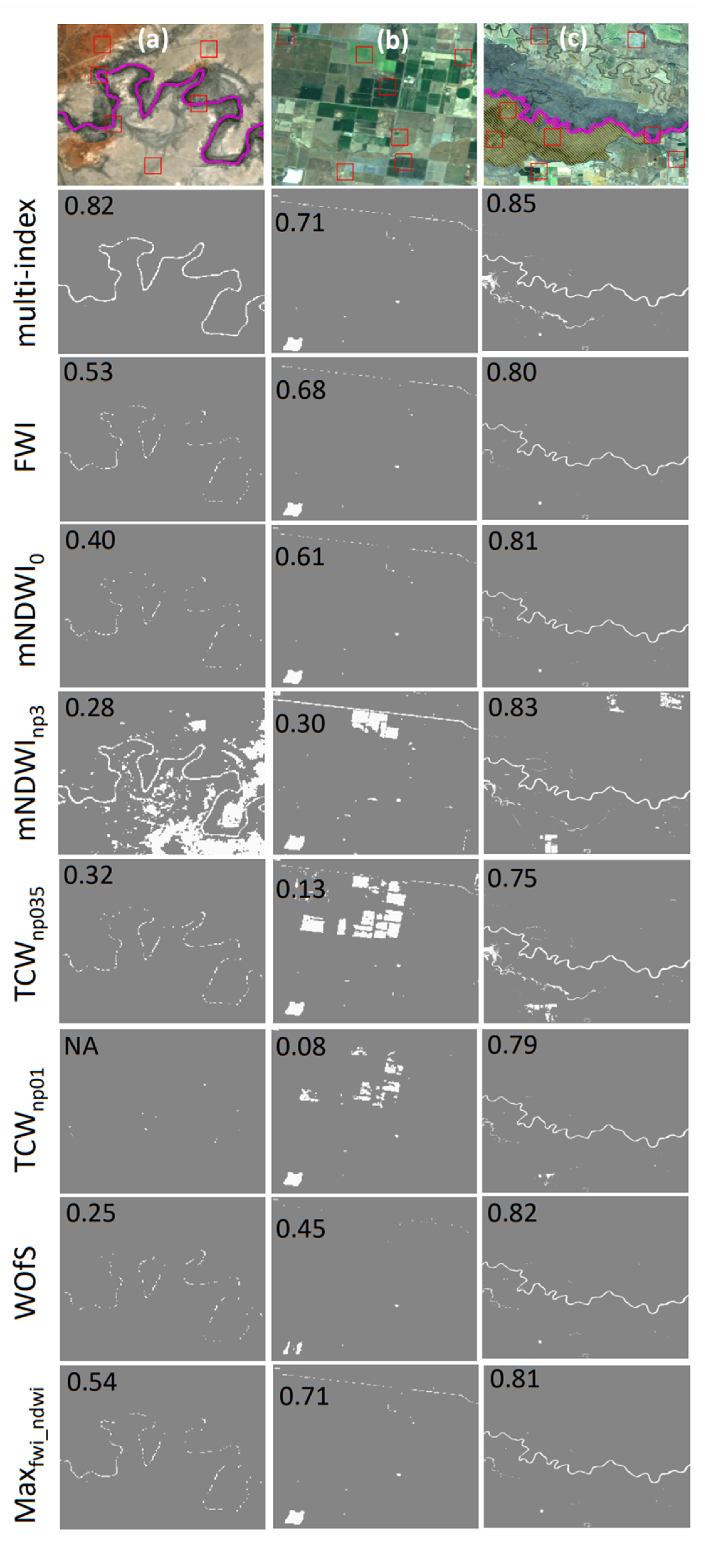
3.1. Visual Assessment

The multi-index two-monthly image for January–February 2019 was inspected across the whole MDB, and checked for any issues across boundaries of the water environments as used in the final rule set for mapping surface water across the MDB: major perennial rivers, wetlands, and the remaining area. Much of the MDB areas showed a seamless transition across boundaries, except for the dark soil floodplain in the west of the MDB. Figure 4a shows a major perennial river (Darling River) along this western section where the river can be at least 35 m wide in sections, as well as the over-mapping of this stream channel based on using mNDWI_np3 within a 100 m buffer along the stream centre (Figure 4b). This can be remedied by reducing the buffer zone to 25 m for mNDWI_np3, and inserting a transition zone from 25 m to 50 m from the centre of the stream channel with mNDWI > −0.15 (i.e., a threshold halfway between −0.3 and 0) (Figure 4c). The width of the river in Figure 4c is now 1–2 pixels, which is a better match to its true width. Apart from scattered pixels at the river bends, the other water indices do not detect this river during this period. Furthermore, despite the Darling River being classified as a major perennial river in the Geofabric, in recent years, parts of it can cease to flow during dry periods [65], as seen here. In the southern section of the MDB, along the Murray River (Figure 4d), the river is almost 100 m wide in sections. The multi-index method here shows that mNDWI_np3 falls within the buffer zone and is 3–4 pixels wide. However, any areas where the geofabric streams do not align properly with the river channel in the Landsat imagery will affect the accuracy of the final product as mNDWI_np3 may over-map water in these areas of mismatch.

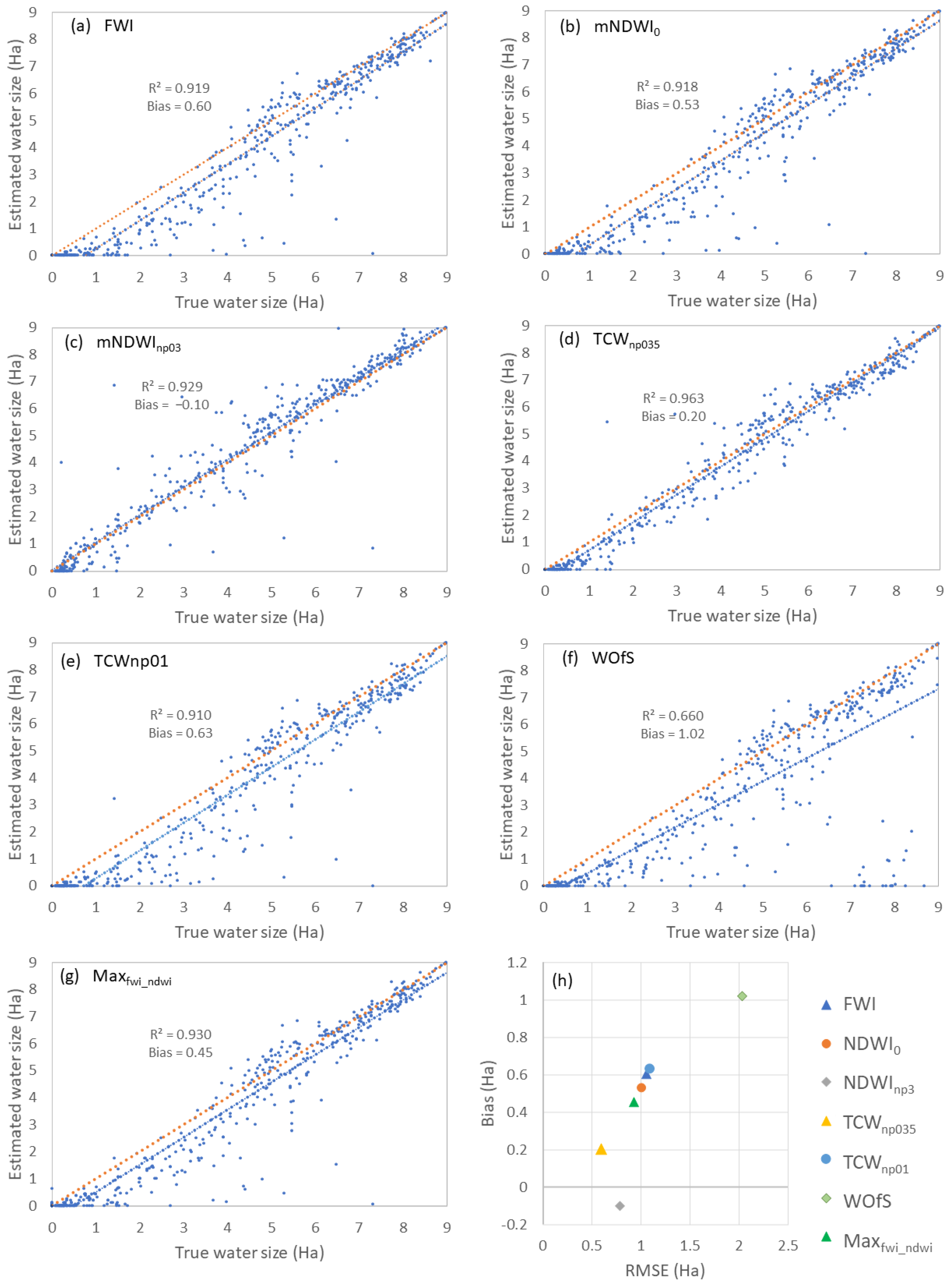
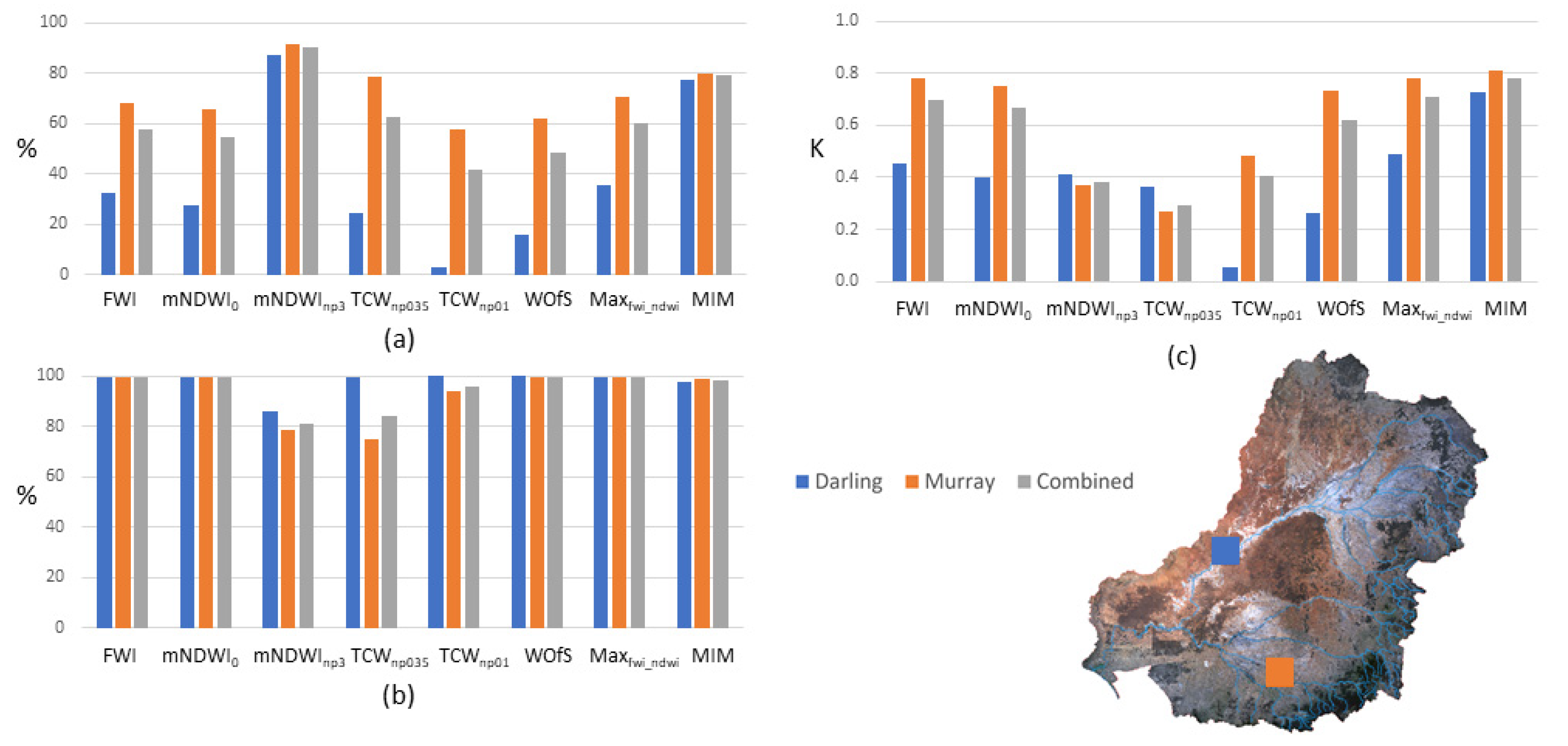
3.2. Assessment from Independent Validation Data

The multi-index method was developed using the validation plots mostly from Fisher et al. (2016) [31]. An additional 40 validation plots were used to provide an independent assessment of the multi-index method and a further comparison with the other indices from Table 1. Approximately 12,000 Landsat pixels were assessed from these independent validation plots with a summary shown in

Table 3. Producer’s accuracy (%) for water and non-water (dry) pixels, as well as the Kappa statistic (K) for each water index from the independent validation plots (refer to Table 1 and Equation (1) for definition of indices). MIM = multi-index method.

Index	Water (%)	Dry (%)	K
FWI	57.66	99.73	0.699
mNDWI0	54.40	99.78	0.674
mNDWInp3	90.30	82.09	0.393
TCWnp035	62.65	84.43	0.294
TCWnp01	41.61	97.23	0.445
WOfS	48.41	99.82	0.623
Maxfwi_ndwi	60.04	99.69	0.716
MIM	79.06	98.50	0.791

. K is notably higher for the multi-index method (0.79), followed by Max_{fwi_ndwi} (0.72) and FWI (0.70). Water pixel accuracy for the multi-index method is 79.1%, which is second to mNDWI_np3 (90.3%). Dry pixel accuracy for the multi-index method is 98.5%, which is lower than FWI, mNDWI₀, WOfS, and Max_{fwi_ndwi}, but still high.

These additional validation plots were extracted from two areas in the MDB located in different environments (Figure 5). The Darling River site is a more arid zone compared to the Murray River site, which is located in an agricultural region with vegetated wetlands. The wet pixel accuracy (Figure 5a), dry pixel accuracy (Figure 5b), and Kappa statistics (Figure 5c) are shown for each site as well as the combined results. As has been seen in the previous results, mNDWI_np3 is best at identifying water pixels for both sites, but this leads to commission errors, as seen by the low dry pixel accuracy. All indices have a lower accuracy for water pixels for the Darling River site compared to the Murray River site. This is because it is a dry arid site with only small and/or narrow water bodies. The dry pixel accuracy for TCW_np035 is the lowest for the Murray River site due to irrigated crops being misclassified as inundated. This low accuracy leads to a low K value for the combined sites and, hence, a poor agreement (0.30). The multi-index method performs consistently well for both the wet pixel (Figure 5a) and dry pixel (Figure 5b) accuracy for both sites, resulting in a high K for the combined sites (Figure 5c).

For a more detailed assessment, three subsets covering the independent validation sites (one from the Darling River site and two from the Murray River site) were extracted and water maps from the multi-index method are compared to the other indices (Figure 6). The Kappa statistic was also calculated from these subsets and are shown in Figure 6. The validation sites used to calculate K for each subset are shown in the true colour images as red squares. Figure 6a shows the Darling River meandering through the middle of an arid region (outlined in magenta). The high-resolution validation image did show the Darling River to be flowing for this area and date. The dark floodplain soils show as a grey colour compared to the surrounding red soil. The multi-index method has a notably higher K statistic (0.82) compared to the other indices. This is because it is able to detect the full length of the Darling River, since mNDWI_np3 is used within the river buffer. However, as can be seen in the water map image for mNDWI_np3, inundation is incorrectly identified through much of the floodplain using this index alone. Max_{fwi_ndwi} is used to map water for the remaining areas of this subset in the multi-index water map, which correctly identifies all pixels as dry. TCW_np01 does not have a K value, since no water was detected in the validation plots containing water.

Figure 6b shows an agricultural region (including irrigation channels and crops) in the Murray River site. Since this subset does not contain major perennial rivers or wetlands, Max_{fwi_ndwi} was used to identify all water in the multi-index method water map. Hence, K (0.71) for Max_{fwi_ndwi} and the multi-index water map are the same. The next highest K for this subset is from FWI (0.68). mNDWI_np3 is best at identifying the irrigation channel traversing the top of this subset; however, it is also misclassifying some of the crops as inundated. The Tasseled Cap Wetness indices are showing the lowest K values, as they are also identifying some crops as inundated.

Figure 6c shows the Murray River passing through the centre of this subset (highlighted in magenta) as well as an ANAE wetland to the southeast of the river (highlighted in orange). The multi-index method clearly shows the Murray River (this is because mNDWI_np3 is being used for major rivers). TCW_np035 is detecting the most water in the ANAE wetland area to the south of the Murray River compared to the other indices. The use of TCW_np035 for wetlands in the multi-index method means it is also seen in the multi-index water map for this area. Similar to the other subsets, K for the multi-index method is highest compared to the other indices (0.85).

Overall, the results show that most indices are capable of mapping surface water with a reasonable degree of accuracy. However, there are situations where mapping is challenging and some indices are more suitable. For example, flooded vegetation is difficult to detect for most water indices; however, TCW_np035 can detect more than the other indices. The challenge is finding validation data identifying flooding extent. One example is for the Barmah-Millewa Forest (whose extent can be seen in Figure 7a) located in the southern section of the MDB, and which is listed as a Ramsar wetland site. This floodplain area consists of open canopy forest (~70%) and woodlands (~29%) [25]. Figure 7b, c, and d show the multi-index method, TCW_np035, and mNDWI_np3 from a Landsat image acquired in December 2010 during a flooding period. The magenta line shows the major river, and orange shows the extent of ANAE wetlands. mNDWI_np3 (Figure 7d) shows much less flood extent within this forested wetland area compared to TCW_np035 (Figure 7c). While the exact extent of flooding during this period is unknown, according to Parks Victoria (2018) [66], 90% of the floodplain was flooded during the 2010–11 hydrologic year (May to the following April). The extent of flooding for the multi-index image (Figure 7b) agrees well with the extent shown in Tulbure et al. (2016) [25] for the flood event for the ANAE wetland area, making the extent shown in the multi-index method within the wetland area plausible. However, less water is identified using the multi-index method in the northern section of the floodplain (Figure 7b) compared to Tulbure et al. (2016) [25], and TCW_np035 (Figure 7c) compares much better. Parks Victoria (2018) [66] also identify this northern section as subject to inundation during large flooding events. Improvements to the wetland layer used to identify wetland extent in the multi-index method is recommended, so it can include these vegetated floodplains.

4. Discussion

While this method has focused on the MDB, it should be applicable to other regions and environments, provided they have the necessary spatial layers (i.e., major rivers and wetlands). This is because the MDB covers a range of environments from arid deserts to alpine forests, and includes a mixture of crops, pastures, native vegetation, and urban areas. Apart from snow cover (which is not addressed here), the multi-index method has been applied to a range of environments. The Geofabric data are available Australia-wide at the same level of spatial detail, which provides the streamline layer necessary for extracting major perennial rivers. The ANAE wetlands layer was only available for the MDB; however, the Directory of Important Wetlands layer [67] is available Australia-wide, which could be applied. Globally, there are a range of layers which could be used to define major streamlines and wetlands: global river networks include MERIT Hydro [68], HydroSHEDS [69], and the global river networks dataset of Yan et al. [70]; the Global Wetlands Map has a selection of wetland layers for the tropics and subtropics [71], while a global wetland layer is also available [72]. Even so, the method described here is to demonstrate the application of targeting commonly used water indices to the environments where they perform best, to help achieve improved results in detecting inundation while minimising the misclassification of dry areas as water.

The multi-index method has not been applied to other regions outside of the MDB; however, previous experience has shown that mNDWI_np3 works well for identifying persistent waterholes within major river channels throughout a number of catchments in northern Australia [40]. mNDWI_np3 was constrained to major river channels due to over-mapping of water in surrounding areas. Comparisons with WOfS found mNDWI_np3 better matched the validation data extracted from high-resolution Google Earth imagery [40]. Previous experience has also found mNDWI_np3 also had difficulty in identifying water within flooded vegetation for areas in northern Australia. However, the example shown in Figure 7 shows TCW_np035 can identify more water in flooded vegetated wetlands; hence, the multi-index approach may potentially improve on this early work. Recent work in central Australia found that mNDWI_np3 was significantly over-mapping water in this arid zone, so mNDWI₀ was applied instead [43]. These previous results provide evidence that different indices work better in different water environments, and further work is required to test the multi-index method in these other regions.

There are limitations in using Landsat imagery to map surface water due to the spatial resolution (30 m) and temporal frequency (8–16 days at best). Water bodies that are smaller than 3 ha will be difficult to identify as surface water in Landsat imagery in complex environments [73]. Inclusion of Sentinel-2 optical imagery in detecting surface water would help due to its relatively high spatial (particularly the visible bands) and temporal resolution compared to Landsat [65]. This is only applicable since the launch of Sentinel-2 (2015), but its archive will grow to become a valuable dataset for future analysis, and it has shown potential, alongside Landsat, for wetland mapping [14].

Cloud cover is always a major problem, particularly when trying to detect surface water before and during the peak of a flood event [74,75]. Furthermore, remnant cloud cover and particularly cloud shadow that is not automatically masked in Landsat imagery is often identified as open water using the water indices [30]. While its extent is not large in Australia, snow can also be mapped as surface water and needs to be masked during the winter months. Dense overhead vegetation will also create a challenge to identifying underlying surface water in optical remote sensing imagery. Synthetic Aperture Radar has already shown to identify flooded vegetation [76] and may be useful to consider when mapping surface water in a complex environment.

5. Conclusions

A good selection of robust indices is already available for mapping surface water using Landsat surface reflectance data. However, targeting the indices to be used in the water environment areas where they perform best can help improve the ability to identify surface water extent. This is the method applied in this study for the MDB. All single indices perform well for mapping surface water extent in the Murray Darling Basin with Kappa statistics ranging from 0.78 (substantial agreement) for WOfS to 0.84 (strong agreement) for TCW_np035 based on all the validation plots combined. However, results improve when indices are used in the environment where they perform best. mNDWI_np3 is good at identifying water along major river channels, but has high commission errors outside these areas. TCW_np035 is best at mapping wetlands, particularly in flooded vegetation, but has high commission errors in cropping regions. FWI and mNDWI₀ (and combined to form Max_{fwi_ndwi}) work well at identifying water in the remaining areas of the MDB basin, with the highest Kappa statistic, and a high accuracy for dry areas (meaning less false identification of water). When these indices are applied to the environments where they perform best, the overall Kappa statistic becomes 0.88, with a water pixel accuracy of 90.5% and a dry pixel accuracy of 94.8%. When applied to an independent validation dataset, the multi-index method still has the highest Kappa statistic of 0.78 (substantial agreement) compared to the other indices. It also performs well in both an arid and agricultural environment. Once a wetlands and major rivers layer is established, this multi-index method is simple to apply, and fast to run across a large area, making it suitable for regional-scale multi-temporal analysis. It was designed to utilise the advantages, as well as minimise the disadvantages, of existing surface water indices commonly used within an Australian environment. However, this method could be applied to any catchment where major streamlines and wetlands (including vegetated floodplain) layers are available or can be created.

References

1. Hughes, D.A.; Kingston, D.G.; Todd, M.C. Uncertainty in water resources availability in the Okavango River basin as a result of climate change. Hydrol. Earth Syst. Sci. 2011, 15, 931–941. [Google Scholar] [CrossRef] [Green Version]
2. Leblanc, M.; Tweed, S.; Van Dijk, A.; Timbal, B. A review of historic and future hydrological changes in the Murray–Darling Basin. Glob. Planet. Change 2012, 80–81, 226–246. [Google Scholar] [CrossRef]
3. Arthington, A.H.; Balcombe, S.R. Extreme flow variability and the ‘boom and bust’ ecology of fish in arid-zone floodplain rivers: A case history with implications for environmental flows, conservation and management. Ecohydrology 2011, 4, 708–720. [Google Scholar] [CrossRef] [Green Version]
4. State of the Climate 2020. Available online: http://www.bom.gov.au/state-of-the-climate/ (accessed on 4 August 2021).
5. Federal Emergency Management Agency. Guidelines and Specifications for Flood Hazard Mapping Partners; Federal Emergency Management Agency: Washington, DC, USA, 2003; p. 49.
6. World Meteorological Organization. Final Report on Flood Hazard Mapping Project; World Meteorological Organization: Geneva, Switzerland, 2009; p. 42. [Google Scholar]
7. Mueller, N.; Lewis, A.; Roberts, D.; Ring, S.; Melrose, R.; Sixsmith, J.; Lymburner, L.; McIntyre, A.; Tan, P.; Curnow, S.; et al. Water observations from space: Mapping surface water from 25 years of Landsat imagery across Australia. Remote Sens. Environ. 2016, 174, 341–352. [Google Scholar] [CrossRef] [Green Version]
8. Peña-Arancibia, J.L.; Zhang, Y.Q.; Pagendam, D.E.; Viney, N.R.; Lerat, J.; van Dijk, A.I.J.M.; Vaze, J.; Frost, A.J. Streamflow rating uncertainty: Characterisation and impacts on model calibration and performance. Environ. Model. Softw. 2015, 63, 32–44. [Google Scholar] [CrossRef]
9. Petersen-Overleir, A. Accounting for heteroscedasticity in rating curve estimates. J. Hydrol. 2004, 292, 173–181. [Google Scholar] [CrossRef]
10. Schumann, G.J.-P.; Brakenridge, G.R.; Kettner, A.J.; Kashif, R.; Niebuhr, E. Assisting flood disaster response with Earth observation data and products: A critical assessment. Remote Sens. 2018, 10, 1230. [Google Scholar] [CrossRef] [Green Version]
11. Wulder, M.A.; Loveland, T.R.; Roy, D.P.; Crawford, C.J.; Masek, J.G.; Woodcock, C.E.; Allen, R.G.; Anderson, M.C.; Belward, A.S.; Cohen, W.B.; et al. Current status of Landsat program, science, and applications. Remote Sens. Environ. 2019, 225, 127–147. [Google Scholar] [CrossRef]
12. Phiri, D.; Simwanda, M.; Salekin, S.; Nyirenda, V.R.; Murayama, Y.; Ranagalage, M. Sentinel-2 data for land cover/use mapping: A review. Remote Sens. 2020, 12, 2291. [Google Scholar] [CrossRef]
13. Kordelas, G.A.; Manakos, I.; Aragonés, D.; Diaz-Delgado, R.; Bustamante, J. Fast and automatic data-driven thresholding for inundation mapping with Sentinel-2 data. Remote Sens. 2018, 10, 910. [Google Scholar] [CrossRef] [Green Version]
14. Lefebvre, G.; Davranche, A.; Willm, L.; Campagna, J.; Redmond, L.; Merle, C.; Guelmami, A.; Poulin, B. Introducing WIW for detecting the presence of water in wetlands with Landsat and Sentinel Satellites. Remote Sens. 2019, 11, 2210. [Google Scholar] [CrossRef] [Green Version]
15. Du, Y.; Zhang, Y.; Ling, F.; Wang, Q.; Li, W.; Li, X. Water bodies’ mapping from Sentinel-2 imagery with modified normalized difference water index at 10-m spatial resolution produced by sharpening the SWIR band. Remote Sens. 2016, 8, 354. [Google Scholar] [CrossRef] [Green Version]
16. Brakenridge, R.; Anderson, E. MODIS-based flood detection, mapping and measurement: The potential for operational hydrological applications. In Nato Science Series: IV: Earth and Environmental Sciences; Springer: Dordrecht, The Netherlands, 2006; Volume 72, pp. 1–12. [Google Scholar]
17. Chen, Y.; Huang, C.; Ticehurst, C.; Merrin, L.; Thew, P. An evaluation of MODIS daily and 8-day composite products for floodplain and wetland inundation mapping. Wetlands 2013, 33, 823–835. [Google Scholar] [CrossRef]
18. Guerschman, J.P.; Warren, G.; Byrne, G.; Lymburner, L.; Mueller, N.; Van-Dijk, A. MODIS-based standing water detection for flood and large reservoir mapping: Algorithm development and applications for the Australian continent. In Water for a Healthy Country National Research Flagship Report; CSIRO: Canberra, Australia, 2011. [Google Scholar]
19. Yamazaki, D.; Trigg, M.A.; Ikeshima, D. Development of a global ~90 m water body map using multi-temporal Landsat images. Remote Sens. Environ. 2015, 171, 337–351. [Google Scholar] [CrossRef]
20. Feng, M.; Sexton, J.O.; Channan, S.; Townshend, J.R. A global, high-resolution (30-m) inland water body dataset for 2000: First results of a topographic–spectral classification algorithm. Int. J. Digit. Earth 2015, 9, 113–133. [Google Scholar] [CrossRef] [Green Version]
21. Zhou, Y.; Dong, J.; Xiao, X.; Xiao, T.; Yang, Z.; Zhao, G.; Zou, Z.; Qin, Y. Open surface water mapping algorithms: A comparison of water-related spectral indices and sensors. Water 2017, 9, 256. [Google Scholar] [CrossRef]
22. Schaffer-Smith, D.; Swenson, J.J.; Barbaree, B.; Reiter, M.E. Three decades of Landsat-derived spring surface water dynamics in an agricultural wetland mosaic; Implications for migratory shorebirds. Remote Sens. Environ. 2017, 193, 180–192. [Google Scholar] [CrossRef] [PubMed] [Green Version]
23. Soulard, C.E.; Walker, J.J.; Petrakis, R.E. Implementation of a surface water extent model in Cambodia using cloud-based remote sensing. Remote Sens. 2020, 12, 984. [Google Scholar] [CrossRef] [Green Version]
24. Pekel, J.F.; Cottam, A.; Gorelick, N.; Belward, A.S. High-resolution mapping of global surface water and its long-term changes. Nature 2016, 540, 418–422. [Google Scholar] [CrossRef] [PubMed]
25. Tulbure, M.G.; Broich, M.; Stehman, S.V.; Kommareddy, A. Surface water extent dynamics from three decades of seasonally continuous Landsat time series at subcontinental scale in a semi-arid region. Remote Sens. Environ. 2016, 178, 142–157. [Google Scholar] [CrossRef]
26. Ko, B.C.; Kim, H.H.; Nam, J.Y. Classification of potential water bodies using Landsat 8 OLI and a combination of two boosted random forest classifiers. Sensors 2015, 15, 13763–13777. [Google Scholar] [CrossRef] [Green Version]
27. Sun, F.; Sun, W.; Chen, J.; Gong, P. Comparison and improvement of methods for identifying waterbodies in remotely sensed imagery. Int. J. Remote Sens. 2012, 33, 6854–6875. [Google Scholar] [CrossRef]
28. McFeeters, S.K. The use of the Normalized Difference Water Index (NDWI) in the delineation of open water features. Int. J. Remote Sens. 1996, 17, 1425–1432. [Google Scholar] [CrossRef]
29. Xu, H. Modification of normalised difference water index (NDWI) to enhance open water features in remotely sensed imagery. Int. J. Remote Sens. 2006, 27, 3025–3033. [Google Scholar] [CrossRef]
30. Feyisa, G.L.; Meilby, H.; Fensholt, R.; Proud, S.R. Automated Water Extraction Index: A new technique for surface water mapping using Landsat imagery. Remote Sens. Environ. 2014, 140, 23–35. [Google Scholar] [CrossRef]
31. Fisher, A.; Flood, N.; Danaher, T. Comparing Landsat water index methods for automated water classification in eastern Australia. Remote Sens. Environ. 2016, 175, 167–182. [Google Scholar] [CrossRef]
32. Singh, K.V.; Setia, R.; Sahoo, S.; Prasad, A.; Pateriya, B. Evaluation of NDWI and MNDWI for assessment of water logging by integrating digital elevation model and groundwater level. Geocarto Int. 2015, 30, 650–661. [Google Scholar] [CrossRef]
33. Crist, E.P. A TM Tasseled Cap equivalent transformation for reflectance factor data. Remote Sens. Environ. 1985, 17, 301–306. [Google Scholar] [CrossRef]
34. Dunn, B.; Lymburner, L.; Newey, V.; Hicks, A.; Carey, H. Developing a tool for wetland characterization using fractional cover, Tasseled Cap Wetness and Water Observations from Space. In Proceedings of the IGARSS 2019–2019 IEEE International Geoscience and Remote Sensing Symposium, Yokohama, Japan, 28 July–2 August 2019; pp. 6095–6097. [Google Scholar] [CrossRef]
35. Donchyts, G.; Schellekens, J.; Winsemius, H.; Eisemann, E.; Van de Giesen, N. A 30 m resolution surface water mask including estimation of positional and thematic differences using Landsat 8, SRTM and OpenStreetMap: A case study in the Murray-Darling Basin, Australia. Remote Sens. 2016, 8, 386. [Google Scholar] [CrossRef] [Green Version]
36. Li, W.; Du, Z.; Ling, F.; Zhou, D.; Wang, H.; Gui, Y.; Sun, B.; Zhang, X. A comparison of land surface water mapping using the normalized difference water index from TM, ETM+ and ALI. Remote Sens. 2013, 5, 5530–5549. [Google Scholar] [CrossRef] [Green Version]
37. Acharya, T.D.; Subedi, A.; Lee, D.H. Evaluation of water indices for surface water extraction in a Landsat 8 scene of Nepal. Sensors 2018, 18, 2580. [Google Scholar] [CrossRef] [Green Version]
38. Ji, L.; Zhang, L.; Wylie, B. Analysis of dynamic thresholds for the Normalized Difference Water Index. Photogramm. Eng. Remote Sens. 2009, 75, 1307–1317. [Google Scholar] [CrossRef]
39. Sims, N.C.; Warren, G.; Overton, I.C.; Austin, J.; Gallant, J.; King, D.J.; Merrin, L.E.; Donohue, R.; McVicar, T.R.; Hodgen, M.J.; et al. RiM-FIM Floodplain Inundation Modelling for the Edward-Wakool, Lower Murrumbidgee and Lower Darling River Systems. Report prepared for the Murray-Darling Basin Authority. In Water for a Healthy Country Flagship; CSIRO: Canberra, Australia, 2014. [Google Scholar]
40. Sims, N.; Anstee, J.; Barron, O.; Botha, E.; Lehmann, E.; Li, L.; McVicar, T.; Paget, M.; Ticehurst, C.; Van Niel, T.; et al. Earth observation remote sensing. In A Technical Report to the Australian Government from the CSIRO Northern Australia Water Resource Assessment, Part of the National Water Infrastructure Development Fund: Water Resource Assessments; CSIRO: Canberra, Australia, 2016. [Google Scholar]
41. Karim, F.; Peña-Arancibia, J.; Ticehurst, C.; Marvanek, S.; Gallant, J.; Hughes, J.; Dutta, D.; Vaze, J.; Petheram, C.; Seo, L.; et al. Floodplain inundation mapping and modelling for the Fitzroy, Darwin and Mitchell catchments. In A Technical Report to the Australian Government from the CSIRO Northern Australia Water Resource Assessment, Part of the National Water Infrastructure Development Fund: Water Resource Assessments; CSIRO: Canberra, Australia, 2018. [Google Scholar]
42. Dutta, D.; Vaze, J.; Karim, F.; Kim, S.; Mateo, C.; Ticehurst, C.; Teng, J.; Marvanek, S.; Gallant, J.; Austin, J. Floodplain Inundation Mapping and Modelling in the Northern Regions, the Murray Darling Basin. In Land and Water; CSIRO: Canberra, Australia, 2016. [Google Scholar]
43. Vaze, J.; Mateo, C.M.; Kim, S.; Marvanek, S.; Ticehurst, C.; Wang, B.; Gallant, J.; Crosbie, R.S.; Holland, K.L. Floodplain inundation modelling for the Cooper basin, Australia. In Geological and Bioregional Assessment Program: Stage 3. Department of the Environment and Energy, Bureau of Meteorology, CSIRO and Geoscience Australia; CSIRO: Canberra, Australia, 2021. [Google Scholar]
44. Jones, J.W. Efficient wetland surface water detection and monitoring via Landsat: Comparison with in situ data from the Everglades Depth Estimation Network. Remote Sens. 2015, 7, 12503–12538. [Google Scholar] [CrossRef] [Green Version]
45. Zhai, K.; Wu, X.; Qin, Y.; Du, P. Comparison of surface water extraction performances of different classic water indices using OLI and TM imageries in different situations. Geo-Spat. Inf. Sci. 2015, 18, 32–42. [Google Scholar] [CrossRef]
46. Ticehurst, C.; Dutta, D.; Karim, F.; Vaze, J. Validation of surface water maps in selected Australian floodplains derived from Landsat imagery using hydrodynamic modelling. In Proceedings of the 22nd International Congress on Modelling and Simulation, Hobart, Australia, 3–8 December 2017; Available online: https://www.mssanz.org.au/modsim2017 (accessed on 9 January 2022).
47. National Water Account. Murray–Darling Basin: Geographic Information. 2020. Available online: http://www.bom.gov.au/water/nwa/2020/mdb/regiondescription/geographicinformation.shtml#geographic_information (accessed on 5 August 2021).
48. Ramsar 2022 Ramsar. Available online: https://ramsar.org/ (accessed on 9 January 2022).
49. The Murray–Darling Basin and Why Its Important. Available online: https://www.mdba.gov.au/importance-murray-darling-basin (accessed on 6 August 2021).
50. CSIRO. Water Availability in the Murray-Darling Basin. A report to the Australian Government from the CSIRO Murray-Darling Basin Sustainable Yields Project; CSIRO: Canberra, Australia, 2008; 67p.
51. Issues Facing the Murray–Darling Basin. Available online: https://www.mdba.gov.au/issues-murray-darling-basin (accessed on 9 January 2022).
52. Dhu, T.; Dunn, B.; Lewis, B.; Lymburner, L.; Mueller, N.; Telfer, E.; Lewis, A.; McIntyre, A.; Minchin, S.; Phillips, C. Digital earth Australia—Unlocking new value from earth observation data. Big Earth Data 2017, 1, 64–74. [Google Scholar] [CrossRef] [Green Version]
53. Lewis, A.; Oliver, S.; Lymburner, L.; Evans, B.; Wyborn, L.; Mueller, N.; Raevksi, G.; Hooke, J.; Woodcock, R.; Sixsmith, J.; et al. The Australian Geoscience Data Cube—Foundations and lessons learned. Remote Sens. Environ. 2017, 202, 276–292. [Google Scholar] [CrossRef]
54. Digital Earth Australia. Available online: https://www.ga.gov.au/dea/home (accessed on 5 August 2021).
55. National Computational Infrastructure Australia. Available online: https://nci.org.au/ (accessed on 5 August 2021).
56. Australian Government, Bureau of Meteorology. Australia Hydrological Geospatial Fabric (Geofabric) Product Guide, Version 3; Bureau of Meteorology Report; Australian Government, Bureau of Meteorology: Melbourne, Australia, 2015.
57. Atkinson, R.; Power, R.; Lemon, D.; O’Hagan, R.; Dovey, D.; Kinny, D. The Australian hydrological geospatial fabric—Development methodology and conceptual architecture. In Water for a Healthy Country; CSIRO: Canberra, Australia, 2008. [Google Scholar]
58. Brooks, S.; Cottingham, P.; Butcher, R.; Hale, J. Murray-Darling Basin Aquatic Ecosystem Classification: Stage 2 Report; Peter Cottingham & Associates Report to the Commonwealth Environmental Water Office and Murray-Darling Basin Authority: Canberra, Australia, 2014. [Google Scholar]
59. Brooks, S. ANAE Classification of the Murray-Darling Basin v2.0; Murray-Darling Basin Authority and Commonwealth Environmental Water Office: Canberra, Australia, 2017.
60. Vaze, J.; Mateo, C.M.; Kim, S.; Marvanek, S.; Keogh, A.; Ticehurst, C.; Teng, J.; Gallant, J.; Austin, J.; Karim, F.; et al. Floodplain Inundation Modelling for the Edward-Wakool Region. In Land and Water; CSIRO: Canberra, Australia, 2018. [Google Scholar]
61. Interim Classification of Aquatic Ecosystems in the Murray Darling Basin Based on the Australian National Aquatic Ecosystems (ANAE) Classification Framework—Wetlands. Available online: http://www.environment.gov.au/fed/catalog/search/resource/details.page?uuid=%7B20B5D7C5-E3D1-47EB-888E-F23940374393%7D (accessed on 5 August 2021).
62. Story, M.; Congalton, R.G. Accuracy Assessment: A User’s perspective. Photogramm. Eng. Remote Sens. 1986, 52, 397–399. [Google Scholar]
63. Landis, J.R.; Koch, G.G. The measurement of observer agreement for categorical data. Biometrics 1977, 33, 159–174. [Google Scholar] [CrossRef] [PubMed] [Green Version]
64. Jensen, J.R. An Introductory Digital Image Processing: A Remote Sensing Perspective; Prentice Hall: Hoboken, NJ, USA, 2005; p. 526. [Google Scholar]
65. MDBA (Murray Darling Basin Authority). A Case Study for Compliance Monitoring Using Satellite Imagery; Murray-Darling Basin Authority: Canberra, Australia, 2018.
66. Parks Victoria. Strategic Action Plan: Protection of Floodplain Marshes in Barmah National Park and Barmah Forest Ramsar Site; Parks Victoria: Melbourne, Australia, 2018.
67. Department of the Environment Directory of Important Wetlands in Australia (DIWA) Spatial Database (Public). Bioregional Assessment Source Dataset. 2015. Available online: http://data.bioregionalassessments.gov.au/dataset/6636846e-e330-4110-afbb-7b89491fe567 (accessed on 13 March 2019).
68. Yamazaki, D.; Ikeshima, D.; Sosa, J.; Bates, P.D.; Allen, G.H.; Pavelsky, T.M. MERIT Hydro: A high-resolution global hydrography map based on latest topography dataset. Water Resour. Res. 2019, 55, 5053–5073. [Google Scholar] [CrossRef] [Green Version]
69. Lehner, B.; Verdin, K.L.; Jarvis, A. New global hydrography derived from spaceborne elevation data. Eos Trans. Am. Geophys. Union 2008, 89, 93–94. [Google Scholar] [CrossRef]
70. Yan, D.; Wang, K.; Qin, T.; Weng, B.; Wang, H.; Bi, W.; Li, X.; Li, M.; Lv, Z.; Liu, F.; et al. A data set of global river networks and corresponding water resources zones divisions. Sci. Data 2019, 6, 219. [Google Scholar] [CrossRef] [PubMed] [Green Version]
71. Global Wetlands. Available online: https://www2.cifor.org/global-wetlands/ (accessed on 15 February 2022).
72. Tootchi, A.; Jost, A.; Ducharne, A. Multi-source global wetland maps combining surface water imagery and groundwater constraints. Earth Syst. Sci. Data 2019, 11, 189–220. [Google Scholar] [CrossRef] [Green Version]
73. Ogilvie, A.; Belaud, G.; Massuel, S.; Mulligan, M.; Le Goulven, P.; Calvez, R. Surface water monitoring in small water bodies: Potential and limits of multi-sensor Landsat time series. Hydrol. Earth Syst. Sci. 2018, 22, 4349–4380. [Google Scholar] [CrossRef] [Green Version]
74. Ju, J.C.; Roy, D.P. The availability of cloud-free Landsat ETM plus data over the conterminous United States and globally. Remote Sens. Environ. 2008, 112, 1196–1211. [Google Scholar] [CrossRef]
75. Ticehurst, C.; Dutta, D.; Vaze, J. A comparison of Landsat and MODIS flood inundation maps for hydrodynamic modelling in the Murray Darling Basin. In Proceedings of the 21st International Congress on Modelling and Simulation, Gold Coast, Australia, 29 November–4 December 2015; Available online: https://www.mssanz.org.au/modsim2015 (accessed on 9 January 2022).
76. Tsyganskaya, V.; Martinis, S.; Marzahn, P.; Ludwig, R. Detection of temporary flooded vegetation using Sentinel-1 time series data. Remote Sens. 2018, 10, 1286. [Google Scholar] [CrossRef] [Green Version]
Figure 1. Location of the Murray Darling Basin within Australia. Location of major rivers, wetlands, large waterbodies, and Landsat image extent containing validation sites (from Section 2.4) within the Murray Darling Basin. The Darling River is shown in dark green and Murray River in bright red. Direction of flow is shown by the dark red arrows.
Remotesensing 14 01158 g001
Figure 2. True area vs. estimated area of surface water within each validation plot with trendline (blue) and 1:1 line (orange) for (a) Fisher’s Water Index (FWI), (b) modified Normalised Difference Water Index (mNDWI) with zero threshold, (c) mNDWI with −0.3 threshold, (d) Tasseled Cap Wetness (TCW) index with −0.035 threshold, (e) TCW index with −0.01 threshold, (f) Water Observations from Space (WOfS), (g) maximum water from FWI and MNDWI0, and (h) Root Mean Square Error and Bias for all indices (refer to Table 1 for a definition of indices).
Remotesensing 14 01158 g002
Figure 3. Multi-Index method developed for mapping surface water across the Murray Darling Basin (SWIR1 and SWIR2 = shortwave infrared bands, fmask = Landsat cloud mask, mNDWI = modified Normalised Difference Vegetation Index, TCW = Tasseled Cap Wetness index).
Remotesensing 14 01158 g003
Figure 4. Examples of the multi-index method within the Murray Darling Basin at the buffer for major perennial rivers. The green and blue boxes show a section of the Darling River and Murray River, respectively. (a) Landsat true colour subset of Darling River, (b) multi-index surface water image for (a) using 100 m buffer zone, (c) multi-index surface water image for (a) using 25 m to 50 m transition zone, (d) Landsat true colour subset of Murray River, (e) multi-index surface water image for (d). The extent of flooding is depicted in white.
Remotesensing 14 01158 g004
Figure 5. (a) Producer’s accuracy (%) for water pixels, (b) producer’s accuracy (%) for dry pixels, and (c) Kappa statistic (K) for each water index from the independent validation plots for the Darling River site, Murray River site, and combined (refer to Table 1 for definition of indices). MIM = multi-index method. Site locations shown in Landsat image.
Remotesensing 14 01158 g005
Figure 6. Comparison of the new multi-index method and the individual indices for three sites across the Murray Darling Basin. (a) Darling River site, (b) agricultural region in Murray River site, and (c) wetland area in Murray River site (refer to Table 1 and Equation (1) for definition of indices). Major perennial streamlines are shown in magenta, ANAE wetlands are outlined in orange, and validation plots used to calculate Kappa (labelled in the inundation images) are outlined in red in the RGB images. The extent of inundation for each index is depicted in white.
Remotesensing 14 01158 g006
Figure 7. (a) Landsat RGB of the Barmah-Millewa Forest in the MDB, (b) water extent from the multi-index method, (c) Tasseled Cap Wetness index (threshold −0.035), and (d) modified Normalised Difference Water Index (threshold −0.3) from December 2010. The magenta lines show the major streams, and orange shows the extent of ANAE wetlands, while the extent of flooding for each index is depicted in white.
Remotesensing 14 01158 g007