
The Improved Three-Step Semi-Empirical Radiometric Terrain Correction Approach for Supervised Classification of PolSAR Data

1
Institute of Forest Resource Information Techniques, Chinese Academy of Forestry, Beijing 100091, China
2
Key Laboratory of Forestry Remote Sensing and Information System, NFGA, Chinese Academy of Forestry, Beijing 100091, China
*
Author to whom correspondence should be addressed.
Remote Sens. 2022, 14(3), 595; https://doi.org/10.3390/rs14030595
Submission received: 9 December 2021
/
Revised: 22 January 2022
/
Accepted: 24 January 2022
/
Published: 26 January 2022
(This article belongs to the Collection Feature Paper Special Issue on Forest Remote Sensing)
Abstract
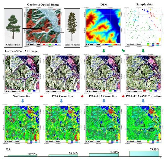
:The radiometric terrain correction (RTC) is an essential processing step for supervised classification applications of polarimetric synthetic aperture radar (PolSAR) over mountainous areas. However, the current angular variation effect (AVE) correction methods of three-step RTC processing are difficult to apply to PolSAR supervised classification because of the problem of interdependence between AVE correction and classification. To address this issue, based on the three-step semi-empirical RTC approach, we propose an improved AVE correction method suitable for the supervised classification of PolSAR. We make full use of the prior knowledge required for supervised classification and RTC processing, that is, samples and elevation data, to calculate the parameters of AVE correction by constructing a weight coefficient matrix. GaoFen-3 QPSI (C-band, quad-polarization) data were used to verify the proposed method. Experimental results showed that the proposed method is available and effective for PolSAR supervised classification. The new method can effectively remove the AVE effect in the PolSAR image, and the overall accuracy of PolSAR supervised classification can be improved about 9% compared to that without AVE correction. For the fine classification of forest types, the AVE correction can improve the classification accuracy by about 20%.
1. Introduction
Due to the characteristics of the side-looking of synthetic aperture radar (SAR) imaging system, SAR images present obvious topographical effects in mountainous areas, which is a great resistance to the application of SAR data. Therefore, radiometric terrain correction (RTC) is an indispensable processing step in the application of SAR in mountainous areas [1]. For polarimetric SAR (PolSAR), the influence of terrain undulations mainly includes three aspects, namely the polarization orientation angle (POA), the effective scattering area (ESA), and the angular variation effect (AVE) [2,3,4,5]. Correspondingly, two or three steps of RTC are usually required to remove the influence of terrain in the PolSAR data [6,7,8].
Among them, the POA correction corresponds to the influence of the slope of azimuth direction, which can affect the intensity of the electromagnetic wave received by radar antenna by changing the polarization direction of the incident wave. The core of POA correction is the calculation of the shift angle of POA. Currently, the most commonly used calculation method is the circular polarization method, which only needs to use the information of the PolSAR data itself [3]. The ESA correction corresponds to the influence of terrain on the scattering area of each pixel of the SAR image. For example, on the front slope, one pixel corresponds to more ground area (i.e., ESA) than it would on the back slope. The larger the ESA, the greater the number of scatterers and the stronger the radiation intensity of the SAR image. In order to eliminate this effect, it is necessary to accurately calculate the ESA of each pixel. Several methods have been proposed and published on this topic [9,10,11,12,13]. These methods can be divided into two types: homomorphic [9,10,11,12] and heteromorphic [4,13]. The homomorphic methods ignore the one-to-many and many-to-one relationships between map and slant range radar geometry. Representative homomorphic methods include projection angle method [10], local incidence angle method [12], etc. The heteromorphic methods represented by the area integral method are the most accurate, but it needs to rely on digital elevation model (DEM) data with higher resolution than SAR data. In addition, the projection angle method is the classic and commonly used method [6,9,12]. For ESA correction, regardless of the method used, DEM data are required to assist in the calculation of local imaging geometry. The AVE correction corresponds to the influence of terrain on the scattering mechanisms and penetration depth, among others [5,7]. This correction step is mainly for vegetation coverage areas, and different vegetation types often require different degrees of correction. At present, the proposed methods can be divided into two categories, empirical methods [14] and semi-empirical methods [5,6,15]. The empirical methods lack the theoretical model basis such as look-up table methods [14]. Although some cases have demonstrated the effectiveness of such methods, their generalizability remains to be verified. The semi-empirical AVE correction methods are the current mainstream method, usually based on a basic model using the n-th power of the cosine of the local incident angle or other angles [5,15,16]. The key problem lies in determining the value of n, which depends on the land cover type, radar frequency, and polarization mode [6,15]. In addition to the completely empirical method to determine the value of n [7], when the land cover type is known, the value of n can be determined automatically by statistical methods such as the minimum correlation coefficient [6], fit [15], etc.
In summary, the POA and ESA corrections only need to be based on the information of the PolSAR data itself or DEM assistance to complete the correction. However, in AVE correction, the land cover type needs to be known in advance to calculate the correction parameter n. This means that AVE correction is difficult to apply to the land cover classification of PolSAR data. Currently, in many studies, AVE correction is usually developed for quantitative parameter estimation such as forest biomass or stock volume estimation [6,7,17]. For some classification applications of PolSAR data, POA and ESA corrections are considered sufficient [6,8,15]. However, this situation should be limited to rough classification (e.g., forest/non-forest) of land cover types in areas with generally complex terrain, and is not suitable for the fine classification (e.g., coniferous/broad-leaved forest) of areas with severely complex terrain. Obviously, when the AVE effect is severe enough to affect the land cover classification of PolSAR data, the conflicting problem of the interdependence of AVE correction and classification should be resolved.
In this study, our objective was to address the negative impact of the AVE effect on the land cover classification of PolSAR data. To this end, we propose a novel RTC method suitable for supervised classification of PolSAR data based on the three-step semi-empirical RTC approach [6]. The new correction method can conveniently eliminate the influence of AVE on the supervised classification of PolSAR data. We innovatively used the training sample data required for supervised classification to assist in the completion of AVE correction, thereby improving the accuracy of PolSAR classification. In addition, the proposed method is demonstrated and analyzed using the PolSAR data of the GaoFen-3 satellite.
2. Methods
2.1. Data Format of PolSAR
For a reciprocal medium illuminated by a monostatic SAR, PolSAR data can usually be represented by a two-dimensional complex matrix format, which is defined as a polarimetric covariance matrix (C3):
where indicates multilook averaging; * denotes conjugate; and SHH, SHV, and SVV are the single-look complex observations of different polarization channels. The polarization covariance matrix is usually obtained from the Level-1 products of airborne or spaceborne PolSAR after pre-processing steps such as calibration and multilook.
2.2. Local Geometry of SAR Imaging
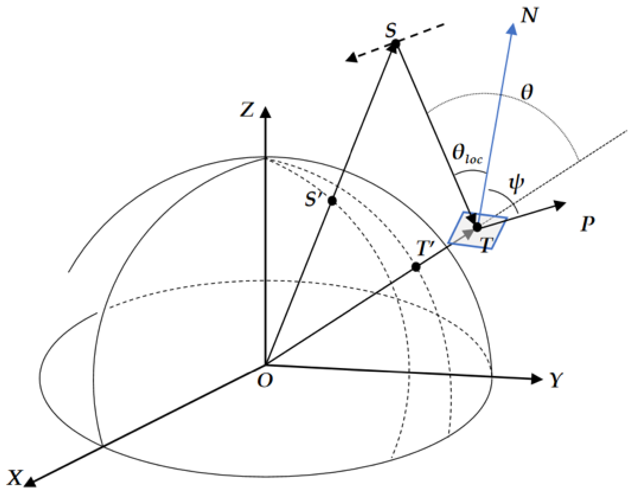
For the RTC process of SAR data, acquiring local imaging geometric information is an indispensable step. Figure 1 shows the local geometry of SAR imaging in an Earth centered rotating (ECR) coordinate system. The projection angle (ψ), local incidence angle (θloc), and incidence angle of a horizontal surface (θ) are the local imaging angle information required by the three-step RTC approach. In order to calculate the angle information, it is necessary to complete the geocoding of terrain correction (GTC) of the SAR data.
Based on precise satellite orbit information, imaging parameters and DEM data, GTC can be performed using the range-doppler position model. Then, we can obtain the geographic location (T) of each pixel in the SAR image and the corresponding sensor location (S). That is, the vectors OT, OS, and TS are known. Based on the DEM data, the normal vector of local surface (TN) is easy to calculate. Finally, the local angle information required by RTC can be calculated based on Equations (2)–(4).
where TP is the vector that perpendicular to the incidence plane [12], and TP = TS × (TS × OT), ∙ denotes the dot product, × denotes the cross product.
2.3. Three-Step Semi-Empirical RTC Approach for PolSAR Data
The three-step semi-empirical RTC approach, which includes the POA, ESA, and AVE correction methods, was developed fully applicable to the PolSAR matrix data [6]. The first step is POA correction. For the C3 matrix, the POA correction can be completed by Equation (5):
where δ denotes the POA shift angle, which can be calculated by the circular polarization method [3].
The second step is ESA correction [6,12]. Based on the C3 matrix after POA correction, the ESA correction can be performed by Equation (6):
It should be noted that the premise of applying Equation (6) is that the backscatter coefficients of different polarization channels of the pre-processed PolSAR data correspond to beta naught (β0) backscatter [4,10].
The third step is AVE correction [5,6,7], which is usually based on a basic model using the n-th power of the cosine of the local incident angle. The correction coefficient of AVE correction is defined as
Since the value of n depends on the land cover type, radar frequency, and polarization mode, for a certain land cover type at a certain radar frequency, the AVE correction of PolSAR data needs to know the n values of the three polarization channels, which can be denoted as nhh, nhv, and nvv, respectively. If this combination of n-values is known, we can obtain the correction coefficient matrix (K) for the C3 matrix, and the AVE correction can be performed:
where ⊕ denotes the hadamard product.
Obviously, the key to AVE correction is the acquisition of n values of different polarization channels. On this point, Zhao et al. [6] proposed the method of the minimum correlation coefficient to determine the optimal n value for a certain land cover type, which is shown in Equation (9):
where σ is the backscattering coefficient of a certain polarization channel after POA and ESA correction, and ρ( ) denotes the correlation function.
2.4. Improved AVE Correction for Supervised Classification of PolSAR
The objective of supervised classification of PolSAR is to obtain the land cover type information corresponding to each pixel of the PolSAR image by training the classifier based on the PolSAR data and sample data. Obviously, there are three key points for supervised classification of PolSAR, namely: PolSAR data, sample data, and classifier. Among them, the most basic is the PolSAR data, which should be calibrated by GTC and RTC. Benefiting from the acquisition of full polarization information, PolSAR data have the potential for fine classification. However, this latent ability is also easily disturbed by other factors, one of which is the AVE effect.
Unlike quantitative applications of PolSAR, for AVE correction of supervised classification, what we need is a combination of n-values suitable for a holistic scene of PolSAR data, rather than n-values for a certain land cover type. Moreover, the land cover type map of the area covered by PolSAR data was our purpose, and may not be a priori knowledge.
In fact, for the AVE correction for the supervised classification of PolSAR data, there is still a lot of prior knowledge that is not used, that is, the sample data required for training the classifier of the supervised classification. If the training samples are relatively evenly distributed under different terrain conditions, we can calculate the n-value combinations of different classes through the training sample data and Equation (9). Assuming that there are a total of M classes, these n-value combinations can form an n-value matrix (N), as shown in Equation (10).
where denotes the n value of the x polarization channel of the m-th class.
Then, a weight matrix (W) reflecting the degree of terrain influence of different classes can be defined, as shown in Equation (11).
where wm represents the weight coefficient of the m-th class, and the sum of the weight coefficients of all classes equals 1. The weight coefficients of different classes can also be set based on the analysis of the sample data of supervised classification. The weight coefficients of different categories should reflect the impact of AVE on the classification results, mainly considering two aspects: the degree of a single pixel affected by AVE (that is, the possibility of a single pixel being misclassified due to AVE) and the number of pixels affected by AVE (that is, the number of pixels that may be misclassified).
In practice, two factors can be comprehensively considered to determine the weight matrix:
- (1)
- The first is the steepness of the terrain where the samples are located, which can be analyzed based on the sample location and DEM data. The slope angle (u) can be calculated using Equation (12).
Based on the slope angle, it can be determined which classes are distributed in the flat terrain area (e.g., u < 3°). Then, the weight factor for the classes of the flat terrain area can be set to zero. For example, for water, building land, and farmland (except terraces) and other land cover types, they are usually distributed on flat terrain. Therefore, the weight coefficients corresponding to these land cover types can be set to 0 or a small value.
- (2)
- The second is the area ratio of different classes, and it should not be difficult to learn the rough ratio after preparing the sample data. Except for the types on flat terrain, the weight coefficient of remaining types can be set according to the area ratio of these types. In addition, if the area ratio of different classes cannot be obtained in the process of preparing sample data, we can consider setting the weight coefficients of different classes to the same value for AVE correction. Alternatively, rough area ratio information can also be obtained based on the classification results of PolSAR data after POA and ESA correction. It should be noted that the area ratio is the most important factor to consider, but the weight coefficient is not necessarily set strictly according to the area ratio. For some categories with a small proportion and strong heterogeneity, the value of n calculated by Equation (9) has a certain uncertainty, so the weight coefficient of these categories can be appropriately adjusted.
Once the weight matrix (W) is determined, the combination of n-values required for AVE correction can be calculated using Equation (13).
where , , and are the combination of n-values that take into account the impact of terrain on different land cover types, so they are suitable for the AVE correction of PolSAR data in the whole scene. Finally, AVE correction can be completed based on Equations (8) and (13).
2.5. Supervised Classification and Evaluation
The supervised classification of PolSAR contains three key points: PolSAR data, sample data, and classifier. First, after the three-step correction, the PolSAR data for classification is ready. Second, the sample data need to be prepared. In this step, we need to conduct a field survey of the PolSAR data coverage area to obtain the information of land cover types. High-resolution optical images (satellites, UAV, etc.) of the same time period can be used to aid the survey. The number of sample data should be large enough and be evenly distributed within the coverage of PolSAR data to be representative and able to overcome the influence of various accidental factors. In addition, the sample data should be divided into two groups (e.g., 50% each), namely, training samples and validation samples. The former is used to train the classifier, and the latter to evaluate the classification effect. Finally, a classifier needs to be chosen. In this study, we used the classic Wishart classifier to perform classification experiments [18]. This classifier only uses the most basic information of PolSAR data. In actual classification applications, more polarimetric decomposition features can be extracted based on PolSAR data, and better classification results may be achieved by using classifiers such as SVM [19].
In addition, the confusion matrix, user accuracy (UA), producer accuracy (PA), overall accuracy (OA), and Kappa coefficient (Kap.) are used to evaluate the classification results of different steps of the three-step RTC approach [19]. If it is assumed that there are a total of N classes, the number of samples of the i-th class is Ai, and the number of pixels in which the samples of i-th class are divided into i-th class by the classifier is Bi, then the PA of the i-th class can be calculated using Equation (14).
Assuming that in all samples the total number of samples classified into i-th class is Ci, then the UA of the i-th class can be calculated using Equation (15).
The OA can be calculated using Equation (16)
and the Kappa coefficient can be calculated using Equation (17).
3. Test Site and Data
3.1. Test Site
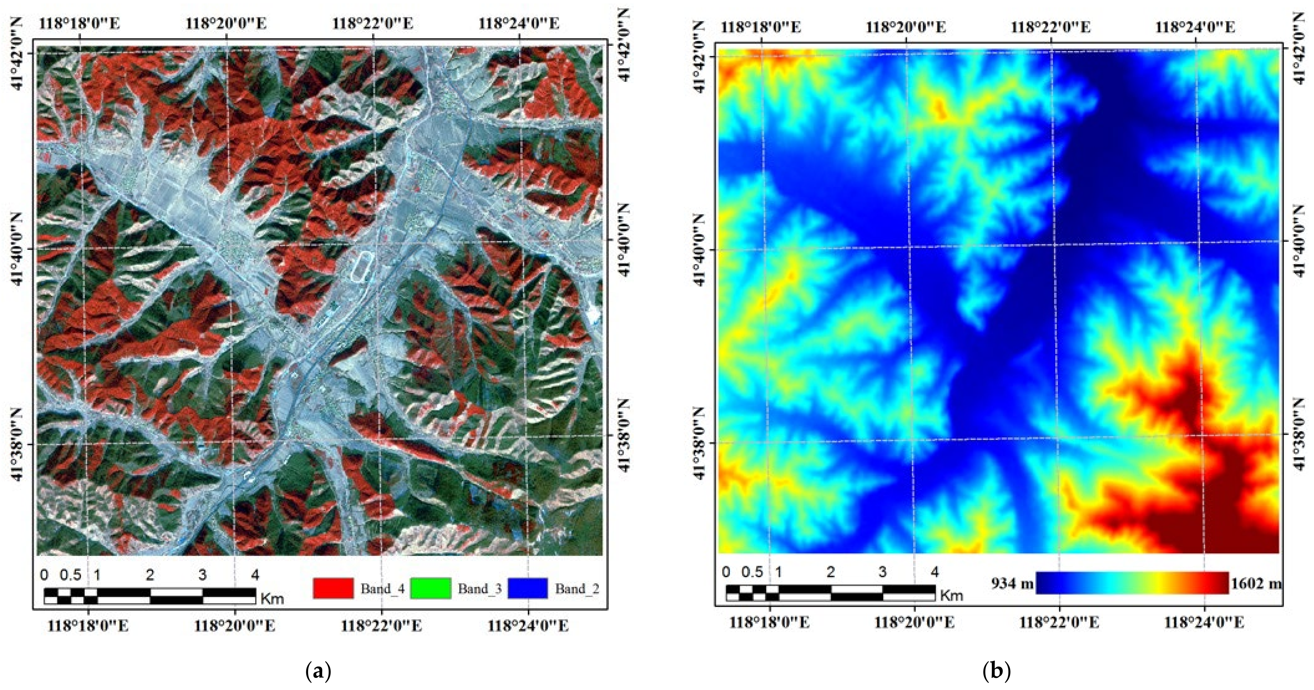
This study was conducted at the test site in Chifeng City, Inner Mongolia, China. The selected 11 km × 10 km study area (Figure 2) is located in the Wangyedian forest farm and contains a town called Meilin (118.3°E, 41.7°N). The slopes in this area are relatively short and steep, with slope angles up to 35°. The elevation range of this area is 934 to 1602 m. This area covers many land cover types such as forests, farmland, construction land, and so on. The forests in this area are plantations, and the main tree species are Chinese Pine (Pinus tabulaeformis Carr) and Larix Principis (Larix principis-rupprechtii May). The former is an evergreen tree species, and the latter is a deciduous tree species. As shown in Figure 3, it is a schematic diagram of a single tree of Chinese Pine and Larix Principis [20]. Although both are coniferous species, the two trees differ in their structural characteristics. The Larix Principis has a very straight trunk with a regular crown shape and internal structure (Figure 3b). However, the trunk of Chinese Pine has a certain curvature, the branches are irregular, and the shape of the crown of different trees is also quite different (Figure 3a).
3.2. PolSAR and Reference Data
One scene from China’s GaoFen-3 PolSAR data was acquired over the test site on 25 September 2019. The data were obtained through the right side view imaging of the descending orbit. It was single-look complex (SLC) data (L1A level) and the observation mode was quad polarization stripe 1 (QPSI). The SLC pixel spacing of the azimuth and range direction were 5.0 and 4.5 m, respectively. In the subsequent processing, SLC data needs to undergo calibration, multilook, and GTC processing. The PolSAR Pauli RGB of the test site after GTC processing is shown in Section 4.2.
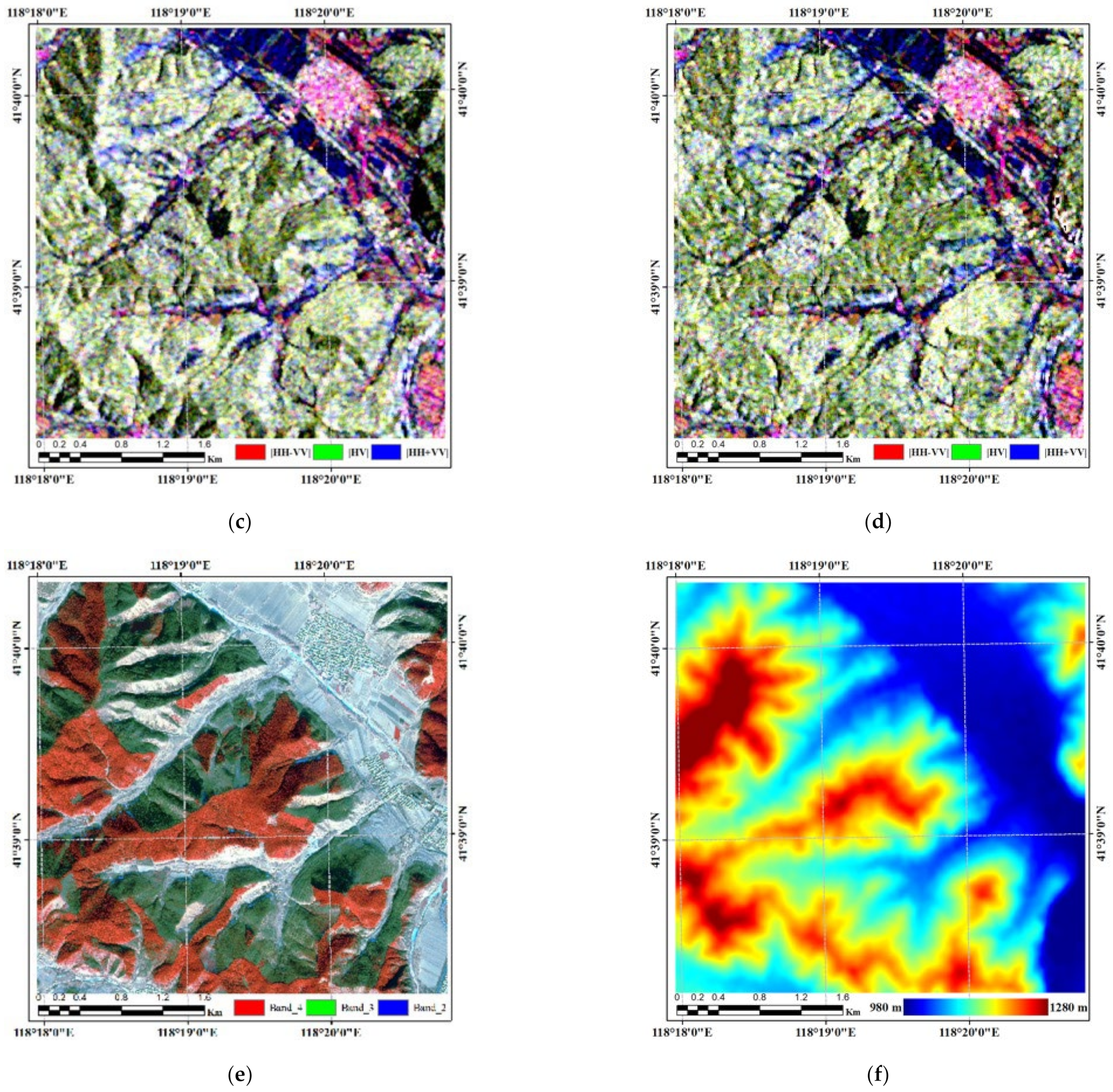
Figure 4a presents the false-color combinations image acquired by China’s GaoFen-2 satellite on 1 January 2019. The image is a fusion of panchromatic image and multi-spectral image, with a high resolution of 0.8 m. Since the acquisition of GaoFen-2 data is in winter, it is easy to distinguish evergreen forests and deciduous forests on the false-color composite image. As shown in Figure 4a, evergreen forests are red, and deciduous forests are brown-green. These features are very helpful for comparative analysis with GaoFen-3’s PolSAR images.
The 1-arcsec SRTM DEM of the test site shown in Figure 4b was used for GTC and to derive local slope information. Taking into account the short slope of the test area and the SLC resolution of PolSAR data, the original 30 m resolution SRTM DEM data were resampled to a 10 m resolution using bilinear interpolation.
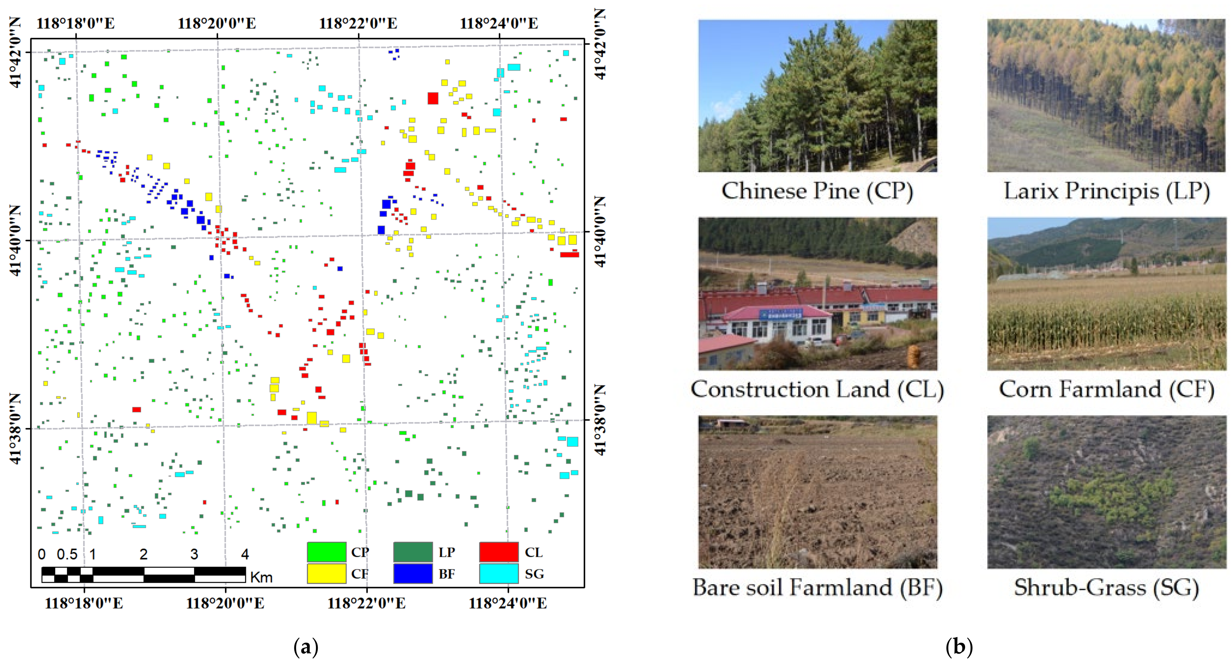
In addition, the field survey in the test site was carried out from 16–28 September 2019. In conjunction with the high-resolution optical image shown in Figure 4a, field survey data, and the classification potential of PolSAR, the sample data required for the classification experiment of this study was obtained, as shown in Figure 5.
The classification system contains six categories including Chinese Pine (CP), Larix Principis (LP), construction land (CL), corn farmland (CF), bare soil farmland (BF), and shrub-grass vegetation (SG). At the end of September, in the test area, the leaves of Larix Principis had turned yellow and gradually fell; most of the crops had been harvested. Among them, most of the corn plants were still left on the farmland after manual picking. Other farmland was plowed into bare soil after harvest. The distribution of the sample data is shown in Figure 5a. The survey photos of different land cover types are shown in Figure 5b.
4. Results
4.1. Pre-Processing of PolSAR
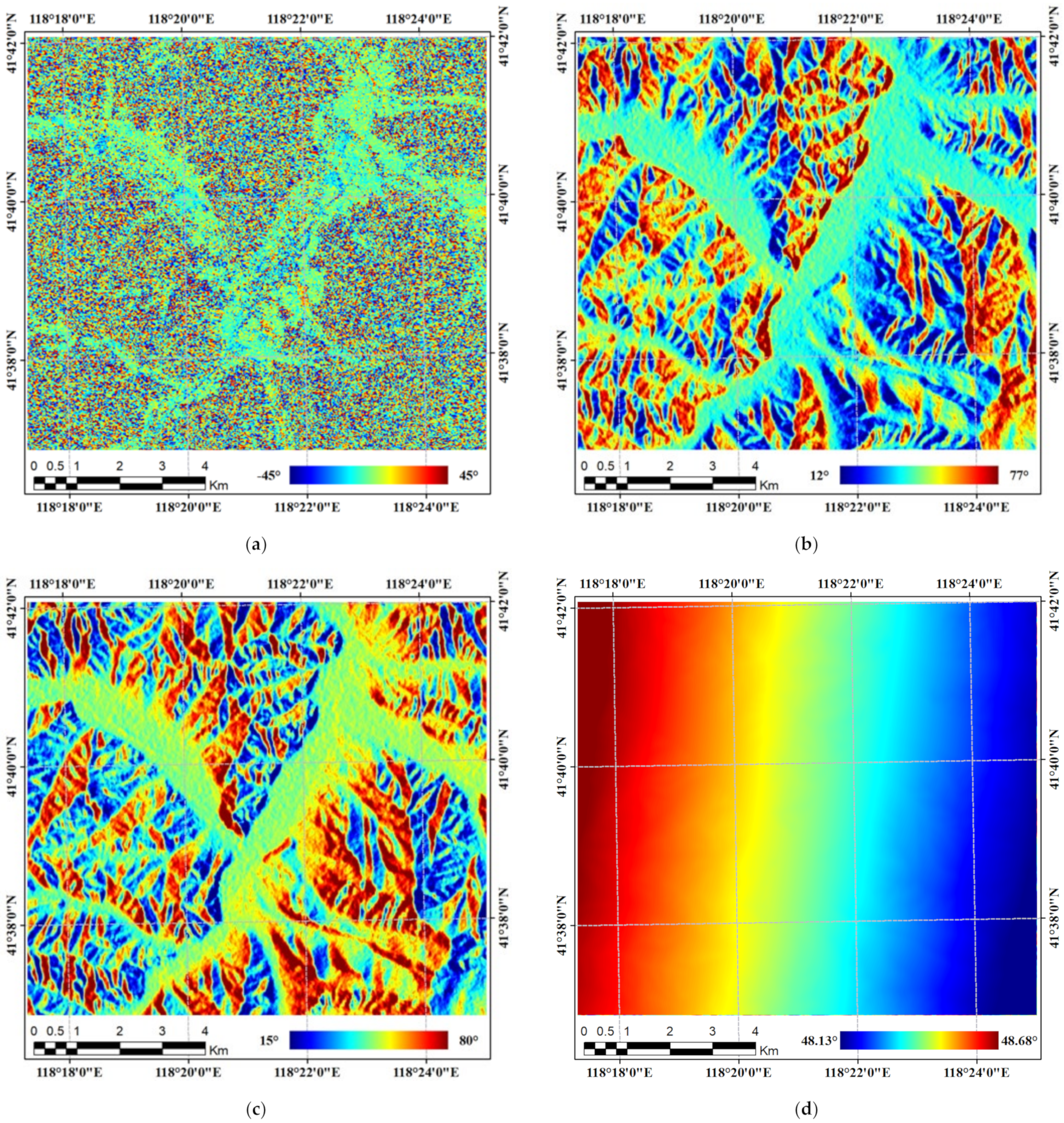
The pre-processing mainly consists of three steps, namely, calibration, multilook, and GTC. First, the calibration is completed based on the parameters in the metadata file (*.meta.xml) provided by GaoFen-3’s L1A data. The multilook step is completed with two looks in the azimuth direction and two looks in the range direction. Then, the multilook complex matrix C3 is obtained, and on this basis, the POA shift angle can be calculated (slant-range radar geometry). Finally, through the GTC process, the geocoded POA shift angle image and the local imaging angle information required by three-step RTC are obtained, as shown in Figure 6. It should be noted that the geocoded PolSAR data and various angle image had the same resolution of 10 m. Inaddition, the slope angle information of the experimental area is calculated using Equation (12). The slope angle information of different land cover types is shown in Figure 7.
In this study, the above pre-processing step was completed using GAMMA software (https://www.gamma-rs.ch/, accessed on 7 December 2021), PolSARpro software (https://earth.esa.int/web/polsarpro/home, accessed on 7 December 2021), and our own program. The processing flow and our shareable program can be found in [21,22].
4.2. Three-Step Semi-Empirical RTC
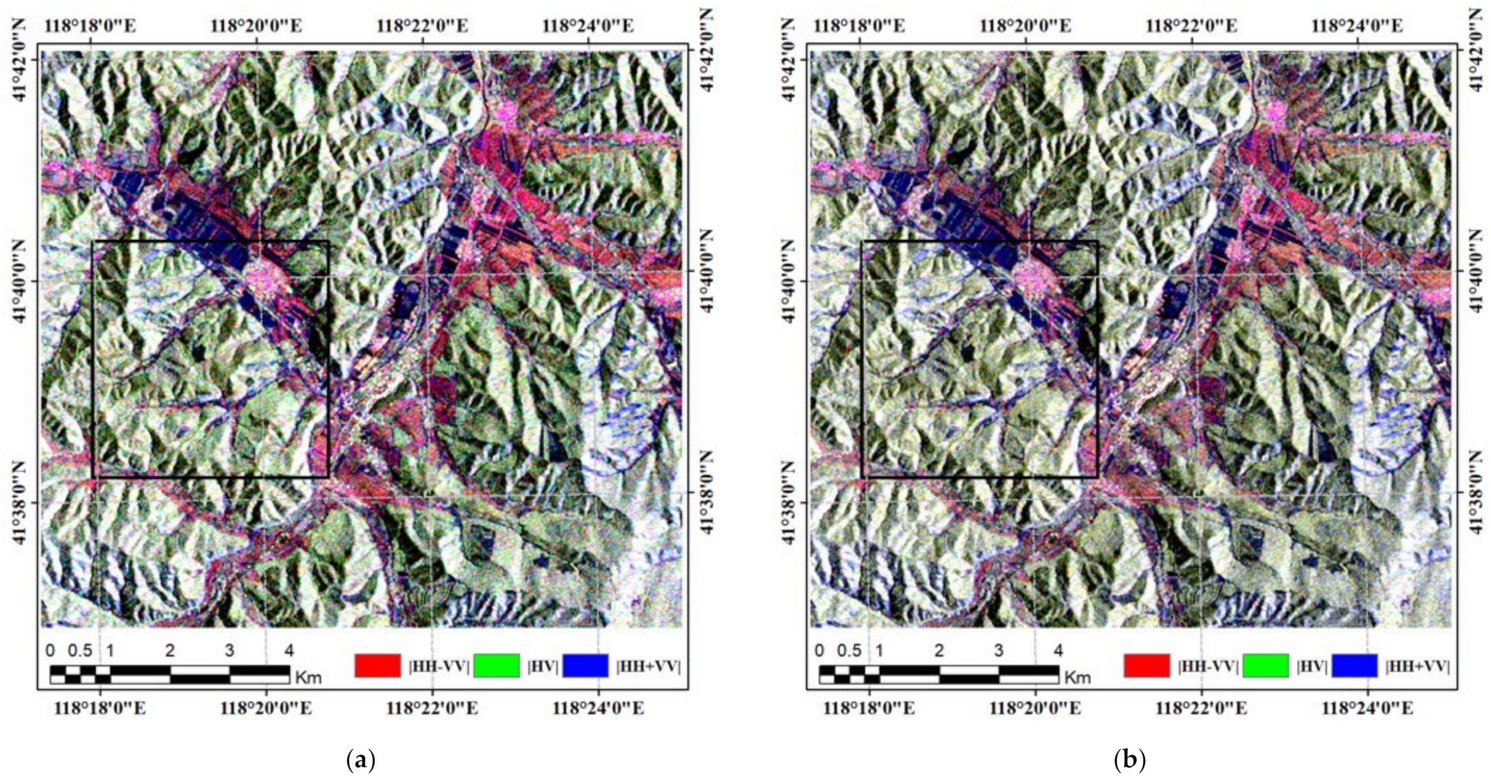
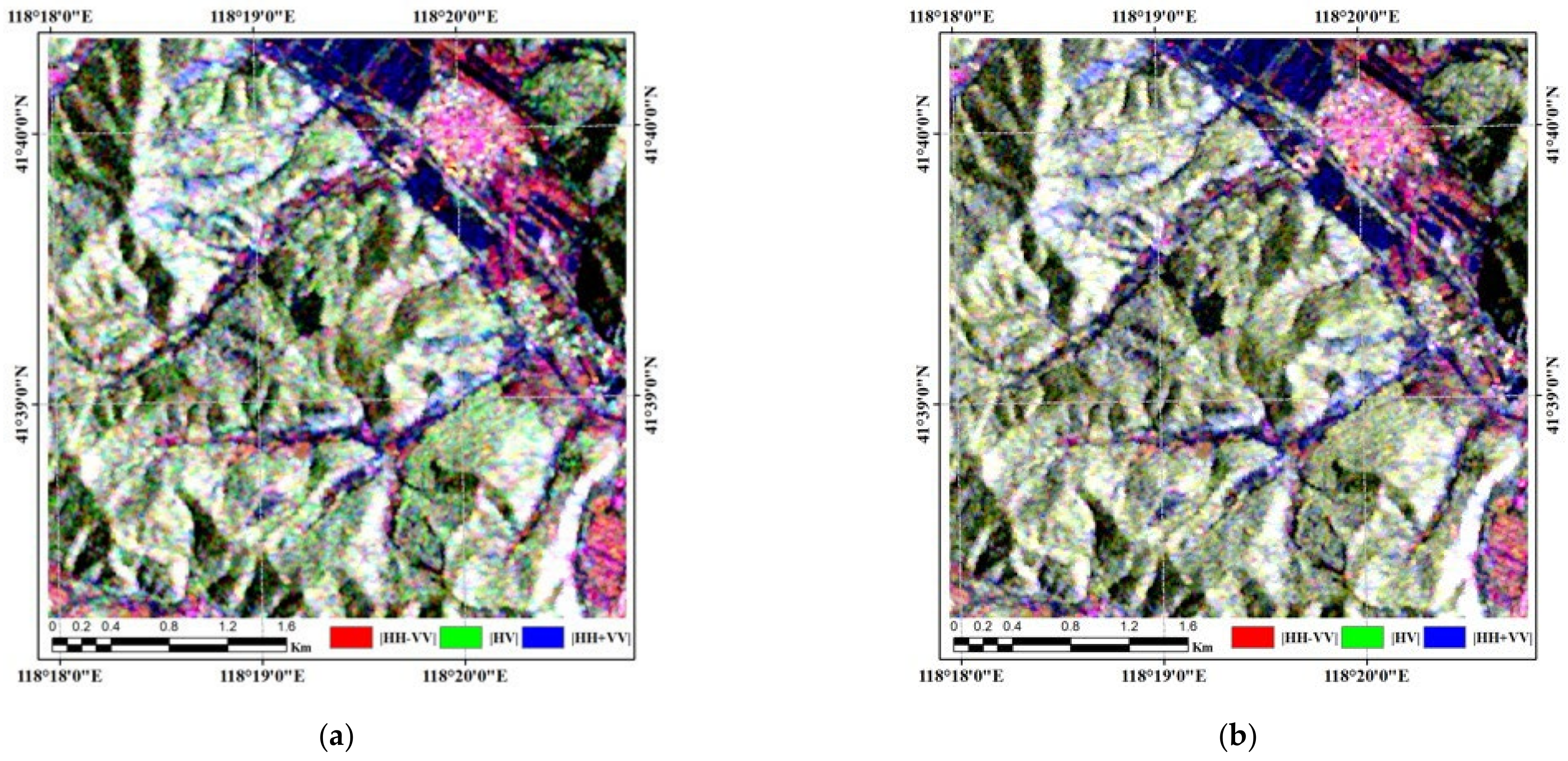
In the first step, the POA correction can be completed by substituting the POA shift angle (Figure 6a) into Equation (5), and the correction result is shown in Figure 8b. Compared to the uncorrected case (Figure 8a), it can be seen that the green spots in the forest area have been eliminated. This reflects the correction of cross polarization. In addition, in order to show the correction effect more clearly, we display an enlarged area in Figure 8 (black polygon) for a more detailed demonstration. As shown in the enlarged images (Figure 9), it can be seen more clearly that the forest area in Figure 9a has a few more green spots than the forest area in Figure 9b. Overall, the effect of POA correction was not obvious. The main reason is that the C-band PolSAR data used in this study have limited penetration of forests and limited influence of azimuth slopes compared with long-wavelength data such as L and P-band.
In the second step, the ESA correction is performed based on the projection angle (Figure 6b) and Equation (6), and the correction result is shown in Figure 8c and Figure 9c. The effect of ESA correction is obvious. It can be seen that the “brightness” of the front slope and the “darkness” of the back slope are obviously more balanced. However, in Figure 8c and Figure 9c, there are still obvious topographic effects that can be seen in the PolSAR Pauli RGB. Moreover, referring to Figure 4a and Figure 9e, the distribution of the two forest types (Chinese Pine and Larix Principis) cannot be seen in Figure 8c and Figure 9c. This means that ESA correction is insufficient for the fine classification of forests using PolSAR data in this study area.
In the third step, the AVE correction needs to be assisted by sample data. First, the classification sample data shown in Figure 5a are randomly divided into two parts: 50% of the samples were used for AVE correction and the training of classifier, and the rest were used as verification samples to evaluate the classification results. Then, the n-value matrix (N) is calculated based on the training samples and the method of minimum correlation coefficient (Equation (9)), as shown in Equation (18):
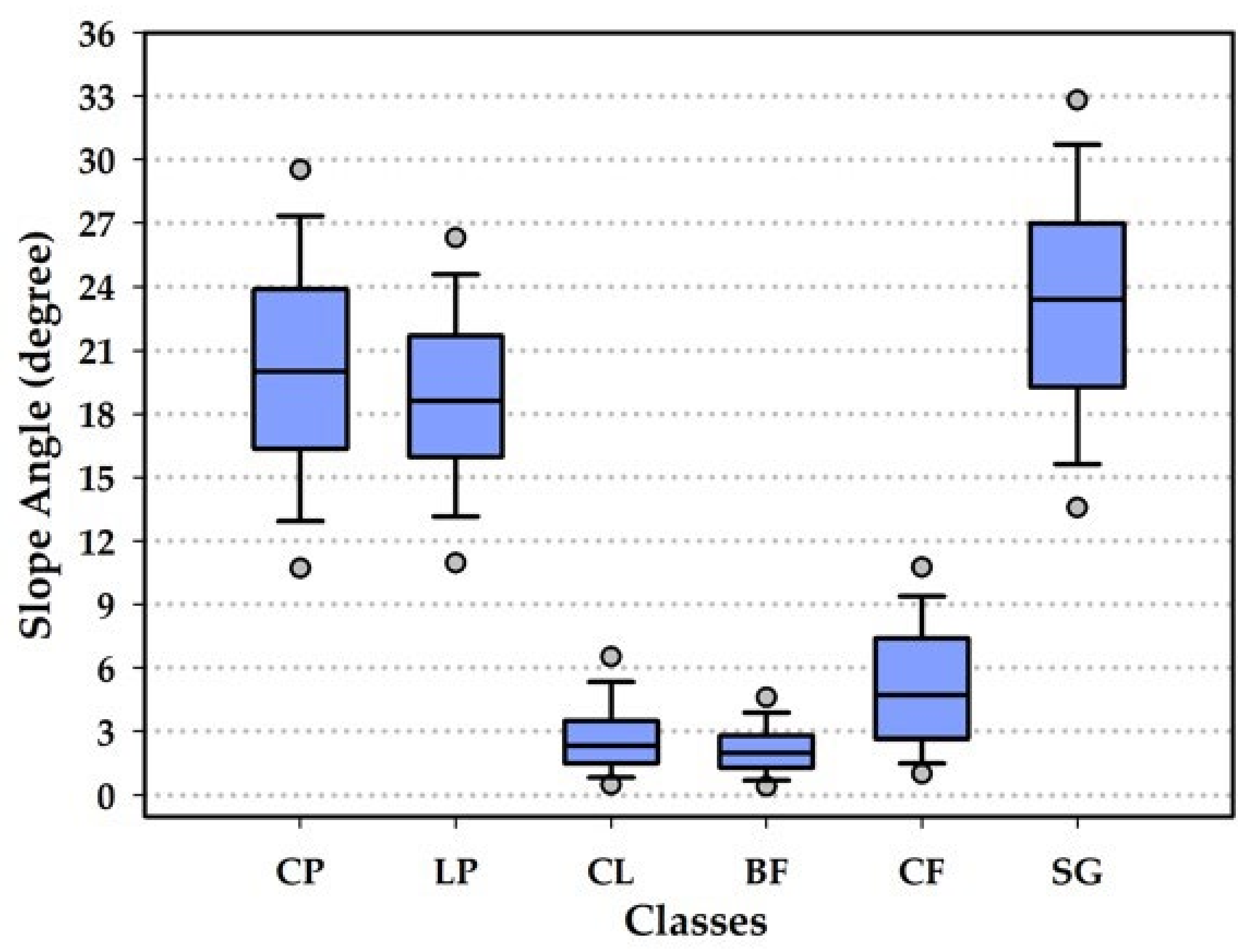
Next, the weight coefficient matrix (W) is determined according to the influence of the AVE phenomenon on different classes. The statistical analysis can be performed on the slope angle information of different categories, as shown in Figure 7. Here, we define areas with an average slope of less than 3° as flat terrain. Obviously, as shown in Figure 7, the construction land and bare soil farmland are distributed in flat terrain. Therefore, we set the weight coefficient of construction land and bare soil farmland to 0.
Among the remaining types distributed in the mountainous areas, forest areas accounted for about 90% of the remaining area, with Chinese Pine and Larix Principis each accounting for approximately half. It should be noted that above 90% was the approximate proportion we obtained in the process of preparing the sample data. Then, the weight coefficient of these two forest types were set to 0.45, and the remaining two classes (corn farmland and shrub-grass vegetation) were set to 0.05 due to their small proportions. In summary, based on the above prior knowledge and analysis, the weight coefficient matrix (W) can be set as:
Obviously, the 90% proportion of forests is rough information obtained through field investigations. The effect of this rough setting on the AVE correction is subjected to a sensitivity analysis in Section 4.4.
Then, the combination of n-values suitable for the PolSAR data of an entire area can be obtained based on the matrix N and W, that is, = 1.11, = 1.00, and = 1.01. Finally, this combination of n-values was substituted into Equation (8) to realize the AVE correction of the entire region, and the correction result is shown in Figure 8d and Figure 9d.
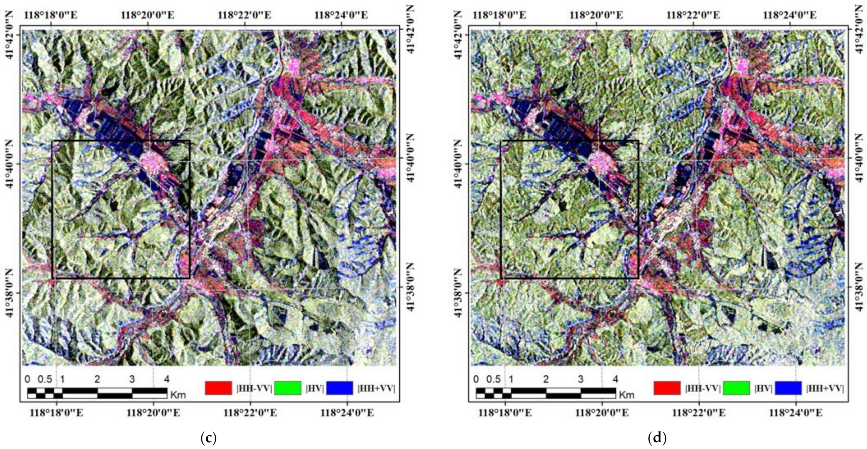
Obviously, the terrain influence was further eliminated compared to the result of the ESA correction. In Figure 8d and Figure 9d, there are almost no traces of terrain undulations. Moreover, the mountainous area clearly presents the characteristics of two types of forest, and their distribution is consistent with the optical false-color composite image (Figure 4a and Figure 9e).
In addition, we used boxplots to perform statistical analysis on PolSAR data of different categories at different correction stages, as shown in Figure 10. By comparing the boxplots of different correction stages, it can be found that the degree of data dispersion of CP, LP, and SG categories was greatly reduced. For example, the range of HH polarization backscatter coefficients for the CP category was about 9 dB without RTC (Figure 10a), while the range after ESA correction was about 6 db (Figure 10g), and the range after further AVE correction was about 4 db (Figure 10g). For the LP category, the corresponding value ranges were 6 dB, 4 db, and 3 db, respectively. The reduction in the degree of dispersion effectively reduces the feature overlap between different classes, which can effectively improve the classification accuracy. Comparing Figure 10g,j, it can be seen that the overlap of CP and LP was reduced from about 50% to 25%.
4.3. Supervised Classification of PolSAR
In order to verify the effectiveness of the proposed method for the supervised classification of PolSAR, we used the Wishart supervised classifier and training samples to perform classification experiments based on PolSAR data in different correction steps. The classification results are shown in Figure 11.
Figure 11a shows the classification results of PolSAR data without terrain correction. It can be seen that the most obvious problem is that there was a large number of misclassified construction land in mountainous areas. After the POA correction, the misclassification of construction land was still serious, but it can also be seen that the mixing of construction land into Larix Principis has diminished (Figure 11b). Immediately after the ESA correction, the problem of misclassification of construction land was significantly improved, and only a small number of pixels in the lower left and right corners of the image were misclassified as construction land (Figure 11c). After the AVE correction, this problem has been further improved (Figure 11d). There is basically no phenomenon of construction land mixed into forest types. In addition, it can be seen from Figure 11a–c that the mixing of the two forest types was also very serious. After AVE correction, the two forest types were relatively clearly separated (Figure 11d).
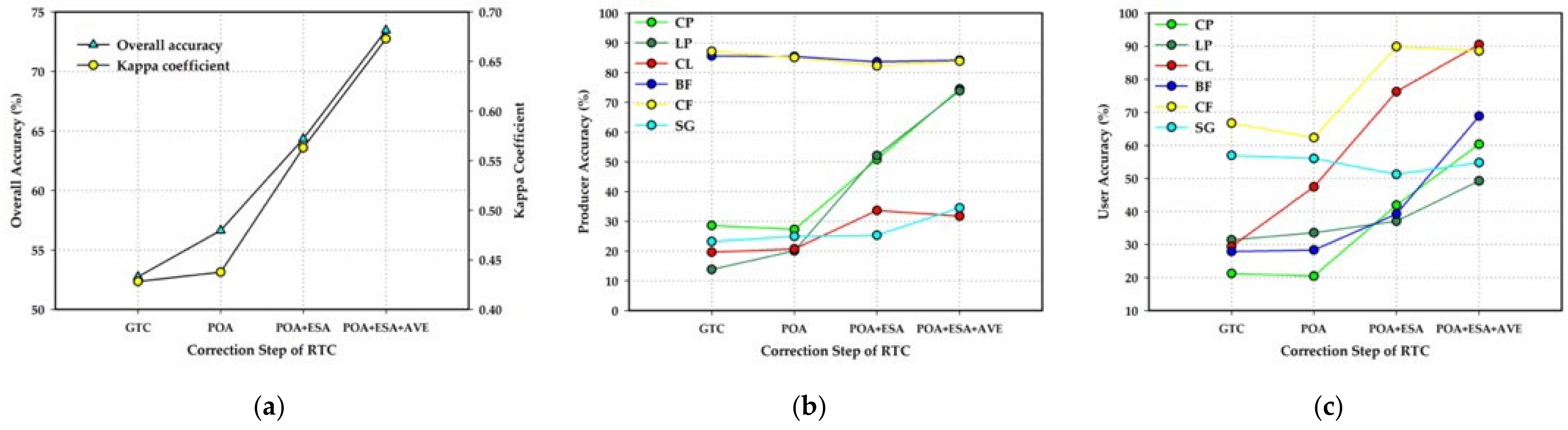
To further quantitatively evaluate the impact of three-step RTC on classification, the confusion matrix of the classification results of different correction steps was calculated based on the verification samples, as shown in Table 1, Table 2, Table 3 and Table 4. The UA, PA, OA, and Kappa coefficient calculated based on the confusion matrix are also shown in the tables and Figure 12.
As shown in Table 1, Table 2, Table 3 and Table 4 and Figure 12a, after three-step RTC, the OA was increased from 52.75% to 73.45%, and the Kappa coefficient increased from 0.4282 to 0.6729. The total increase of OA was about 21%, and the contribution of POA, ESA, and AVE correction was 4%, 8%, and 9%, respectively. For the Kappa coefficient, the total increase was about 0.25, while the contribution of POA, ESA, and AVE correction was 0.01, 0.13, and 0.11, respectively. By comparing the PA and UA of different land cover types, it can be seen that the two categories with the greatest increase in PA were Chinese Pine and Larix Principis, and the two categories with the greatest increase in UA were Chinese Pine and construction land, and the accuracy increase was about 40%. The contribution of AVE correction to the above 40% increase was around 20%. These results illustrate the importance of RTC for PolSAR classification, and AVE correction is also an indispensable step of RTC for PolSAR classification.
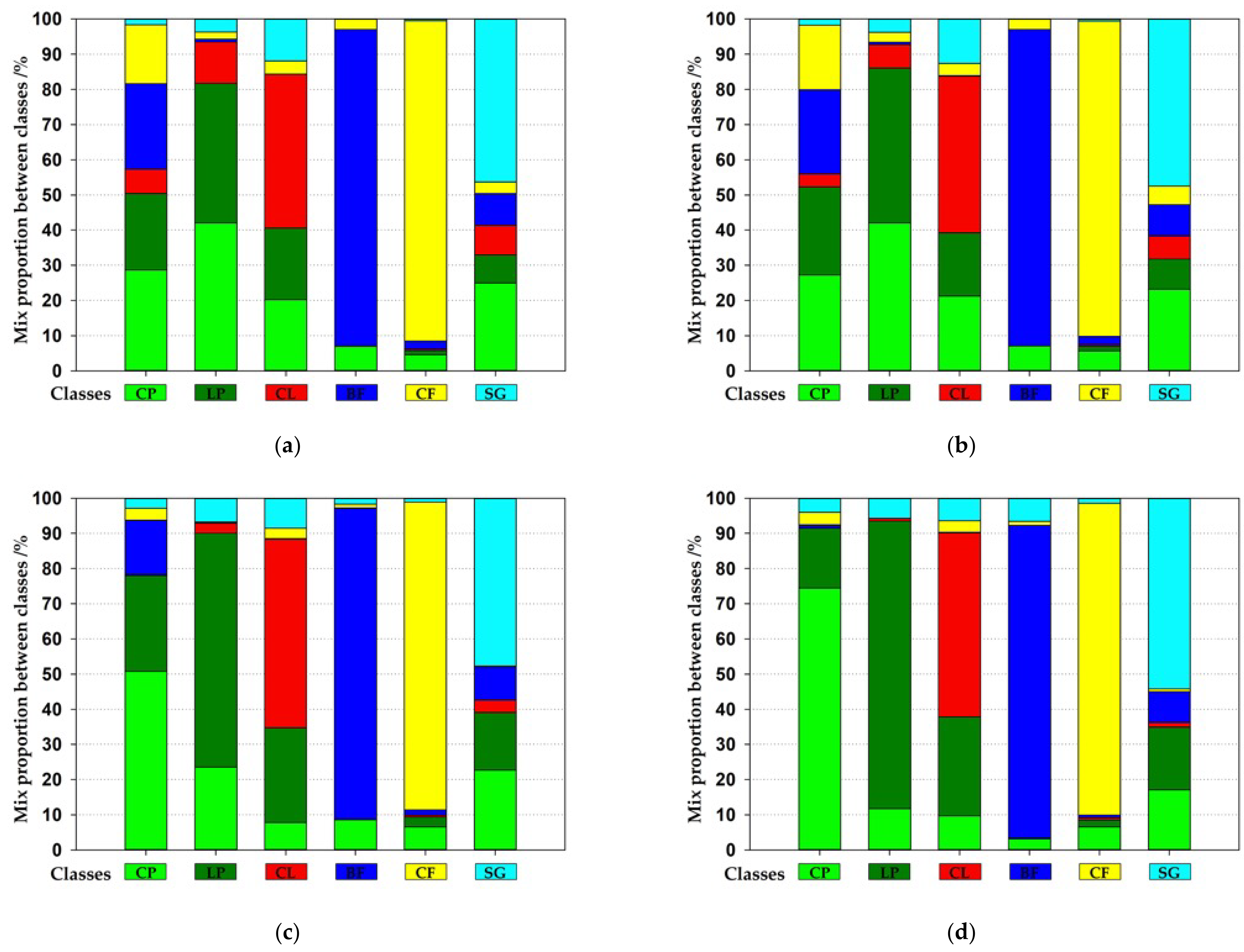
To visually show the influences of different correction steps on PolSAR classification, the confusion matrix was transformed into a histogram of mixed proportion between classes, as shown in Figure 13. In Figure 13, for the column bar of certain class, the length of the bar represents the proportion of each class with regard to the total samples of this class. For this class itself, the length represents PA, and for other classes, it is the misclassification ratio. First, for the two forest types, in addition to the misclassification between themselves, the main mixed classes were bare soil farmland and construction land. The former mainly occurs on the back slope because of the low backscatter coefficient caused by the terrain, and the latter mainly occurs on the front slope because the terrain causes the high backscatter coefficient. This problem was suppressed to a certain extent after POA and ESA correction, and was completely resolved after AVE correction. Second, for construction land, it can be seen from Figure 13 that a large number of samples of these types were classified as forest types. Moreover, after three correction steps, the mixing situation had not been significantly improved. The main reason is that the mixing occurs mainly on flat terrain, which is not a problem that can be solved by terrain correction. Next, for the two types of farmland, they were also very little affected by the terrain, so they maintained high classification accuracy (close to 90%) in different correction steps. Finally, for shrub-grass vegetation types, after three steps of correction, nearly half of the samples were still misclassified as bare soil farmland and forest. The main reason is that the spatial heterogeneity of shrub-grass is large compared with other land cover types. For example, when there are many lush shrubs, the polarization features of shrub-grass are close to forest, and when there are few shrubs and grass is sparse, the polarization features of shrub-grass is close to bare soil.
4.4. Sensitivity Analysis of Weight Matrix
For the AVE correction method proposed in this paper to be applied to PolSAR supervised classification, the setting of the weight matrix is obviously the most critical. The weight matrix is directly related to the determination of the n-value combination in the AVE correction, thereby affecting the effect of the subsequent AVE correction and the final classification accuracy. However, in this paper, the determination of the weight coefficient depends on certain prior knowledge, and is not calculated through strict mathematical formulas. This means that the weight matrix contains some uncertainty, and how the uncertainty affects the subsequent PolSAR classification needs to be further clarified. Therefore, we performed a sensitivity analysis of the weight matrix in this section.
In this paper, as shown in Equation (19), the weight matrix contains six weight coefficients. Obviously, it is difficult to analyze the impact of the final classification accuracy of the changes in the six weight coefficients at the same time. Therefore, only the most important weight coefficients in the weight matrix are analyzed here. First, it is relatively clear that the weight coefficients of CL and BF are set to 0, so the sensitivity analysis does not consider the changes of these two weight coefficients. Second, since the CF and FG categories have a relatively small proportion in the entire region, the weight coefficients of these two categories are considered as a whole when doing sensitivity analysis, and the weight coefficients of these two categories are equal by default. With the above restrictions, if we assume that the weight coefficient of CP is x and the weight coefficient of LP is y, then the weight matrix is:
where x∈[0, 1], y∈[0, 1], and x+y∈[0, 1].
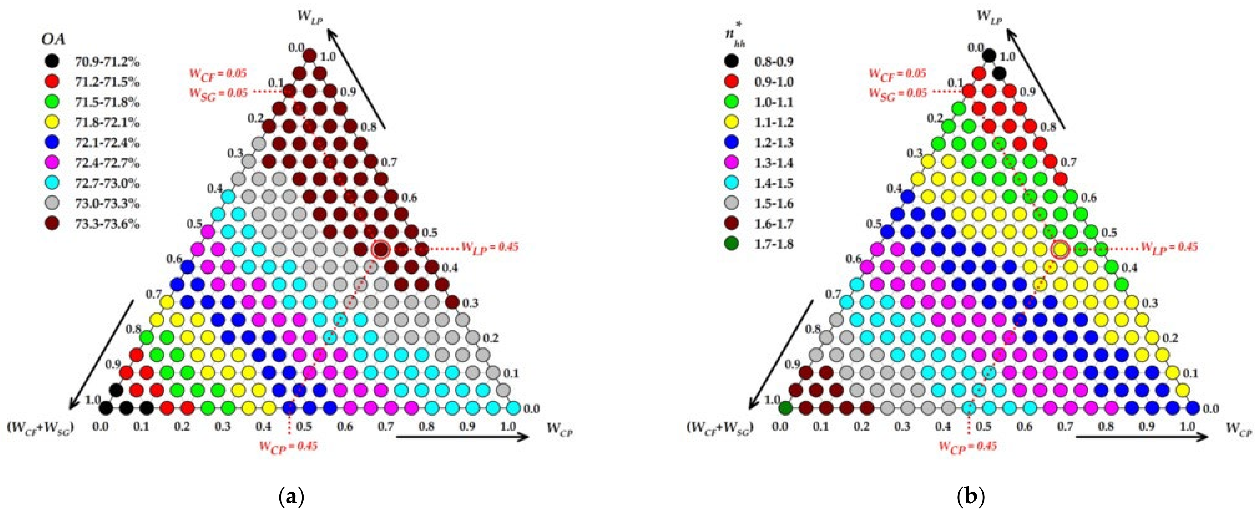
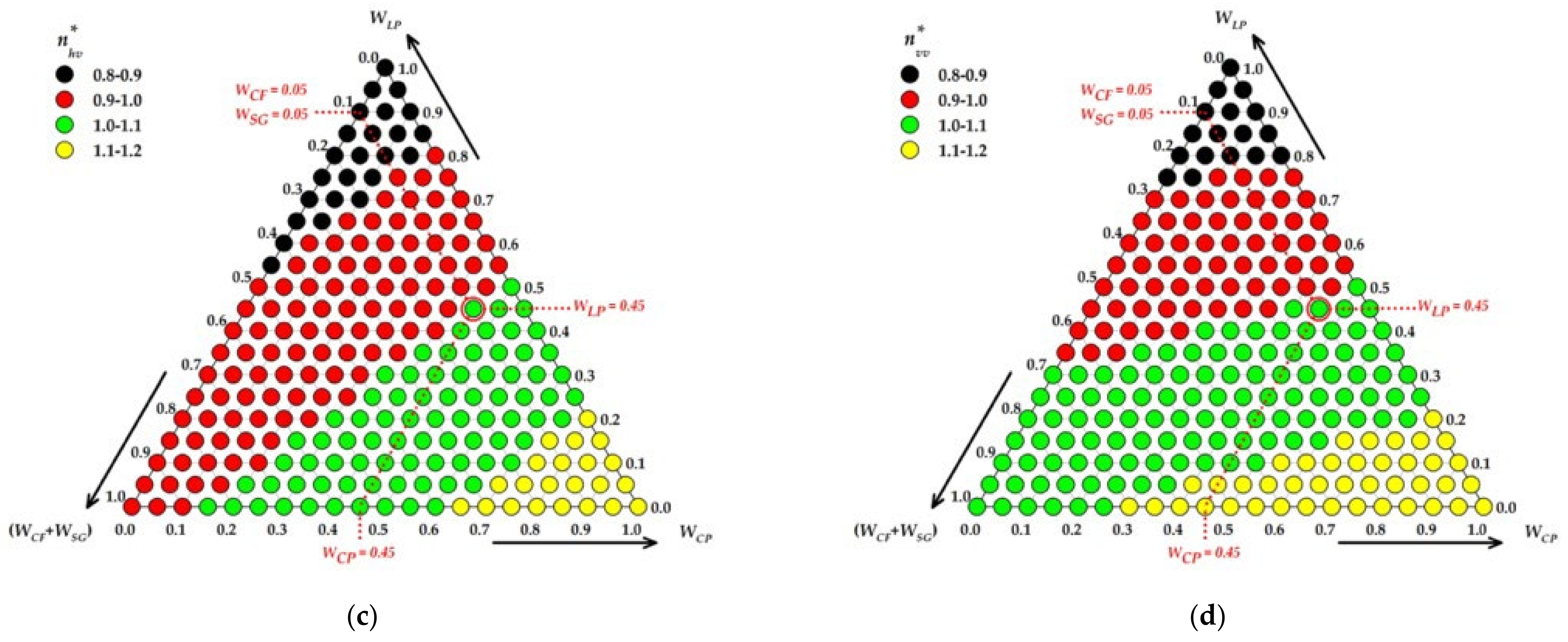
Based on Equation (20), we calculated the n-value combination of AVE correction and overall accuracy of PolSAR supervised classification corresponding to all weight matrices with a step size of 0.05. The analysis results are shown in Figure 14.
As can be seen in Figure 14a, the weight matrix we determined according to the prior knowledge (i.e., Equation (19)) corresponded to the group with the highest overall accuracy (73.3–73.6%). To a certain extent, this shows that the weight coefficient setting method adopted in this paper is reasonable.
However, it should be noted that the sensitivity between the overall accuracy of classification and the weight matrix was not high. First, a wide range of weight coefficient combinations could achieve a high overall accuracy of classification (73.3–73.6%) such as in the case of WLP = 1. Second, the overall accuracy of classification did not vary widely, only about 3% (70.9–73.6%). The main reason is that the weight matrix does not directly affect the final classification accuracy. In other words, the final classification accuracy is directly affected by the n-value combination in the AVE correction, which is obtained by multiplying the weight matrix and the n-value matrix (Equation (18)). This process is complicated, and the difference in the n-value combination obtained by multiplying the two weight matrices with great differences by the n-value matrix is not necessarily large, and may even be equal.
Comparing Figure 14b–d, it can be seen that the variation range of was larger, that is, 0.8–1.8; and the variation range of and was smaller, that is, 0.8–1.2. Obviously, the classification accuracy is mainly affected by the change of . This can also be verified by comparing Figure 14a,b.
Through the above analysis, some preliminary understanding can be obtained. First of all, the sensitivity between the weight matrix and the classification accuracy is not strong, and the deviation of the weight coefficient of about 0.1 corresponds to the classification accuracy deviation of basically no more than 0.3%. This also shows that the setting of the weight matrix can tolerate a certain uncertainty. Second, the above phenomenon does not mean that the weight matrix can be set arbitrarily. However, in the experiments of this paper, the classification accuracy corresponding to different weight matrices had a maximum deviation of only 3%. However, it should be noted that this result is limited by the n-value matrix corresponding to the data in this paper. When the n-value matrix changes, the classification error caused by the uncertainty of the weight matrix may be larger.
5. Discussion
By making full use of the prior knowledge available in the supervised classification (i.e., samples data) and RTC process (i.e., DEM data), we developed an improved version of the three-step RTC approach for supervised classification of PolSAR. Although the experimental results verify the effectiveness of the proposed method, the advantages and disadvantages of the proposed method, some key issues and future developments still need to be discussed.
The effect of topography on PolSAR classification is clearly an issue, but there has not been much research devoted to this issue. Existing terrain correction methods mainly focus on the quantitative application of PolSAR, especially biomass estimation [5,6,7,17]. In the existing research and application, there are three typical strategies to deal with the terrain problem in PolSAR classification. (1) Ignoring the effect of the AVE phenomenon on classification, only POA or ESA corrections were performed on the PolSAR data [8,23]. This strategy is useful for generally complex terrain or coarse classification, but is insufficient for severely complex terrain or fine classification. For example, as shown in Figure 10g, after ESA correction, the forest and construction land were well differentiated, but CP and LP within the forest were still mixed together. Clearly, without AVE correction, both the classification potential and accuracy of PolSAR data are affected. (2) Strategies for hierarchical classification and stepwise correction [15]. First, separate the types on the flat terrain; next, complete the preliminary RTC processing (such as ESA correction); then, separate the types that have not been affected by the terrain effect; finally, assume that the remaining types in the feature space are separable, and make finer terrain corrections (such as AVE corrections) for the remaining terrain types. The problem with this type of approach is that it assumes that at each step, there are some classes that are not characteristically confused with other classes. For classes in flat terrain, this assumption may be satisfied, and the results of Figure 12 in this paper also support this assumption. However, for classes distributed in mountainous areas, stepwise correction cannot solve the problem of interdependence between fine terrain correction and fine classification. Moreover, this approach makes the classification process more complicated and limits the user’s choice of classifiers. (3) Coupling terrain corrections into the interior of the classification algorithm [24]. This method does not correct for the entire polarimetric SAR data (e.g., C3 matrix), but for a feature used for fine classification. Therefore, only specific scenarios and specific classification methods can be applied. For example, the classification method for coniferous and broad-leaved forests based on the parameters of the Stokes vector [24]. In contrast, the method proposed in this paper is relatively independent in the PolSAR supervised classification process, and the correction algorithm does not affect the user’s choice of polarization features and classifiers at all. This is one of the advantages of our method. In addition, the proposed method in this paper is theoretically applicable to polarimetric SAR data of different frequencies because the underlying method for calculating the n value in this paper is the minimum correlation coefficient method (Equation (9)), which does not depend on the variation law of the scattering mechanism at a specific frequency [6]. However, it is definitely necessary to use more PolSAR data of other frequencies to verify the effectiveness of the method proposed in this paper.
Moreover, for AVE correction, the core difficulty is the determination of the value of n for three polarization channels, that is, a total of three unknown parameters. Although we know that the value of n depends on the land cover types, radar frequency, and polarization mode [6,15], it is difficult to determine the value of n suitable for the classification of PolSAR based on this simple indication. For example, for the C-band PolSAR data in this paper, the n value of forest type was around 0.8–1.2 (Equation (18)), and there were large differences between different forest types, but not much between different polarizations. However, for the L-band PolSAR data in [6], the n value of forest type was around 0.45, and the difference between different polarizations was large. In this paper, we transformed the problem of determining the value of n into a problem of determining the weight coefficient matrix through the proposed new method. It should be noted that the number of unknown parameters in the weight coefficient matrix is equal to the number of categories, which is usually greater than 3. Nevertheless, the difficulty of determining the weight coefficient matrix is much easier than directly determining the value of n. The main reason is that the weight coefficient has a clear meaning than the value of n, that is, it represents the extent to which the PolSAR data of a certain land cover type is affected by the terrain. When the influence of terrain is small, the weight coefficient is small, and when the influence of terrain is large, the weight coefficient is also large. In other words, the weight coefficient reflects the influence of terrain on the final classification result. According to the method proposed in this paper, users only need to master a small amount of prior knowledge (slope angle, rough area of different classes, etc.) to determine the weight matrix. The sensitivity analysis of Figure 14a can also help the user to set the weight matrix. For example, if we assume that the area ratio of CP, LP, and CF + SG is 1:1:1, the corresponding weight matrix is:
As can be seen from Figure 14a, the total classification accuracy corresponding to Equation (21) was around 72.7%, which is also a good result.
In addition, a problem that needs to be noted is that the same combination of n-values (Equation (13)) is used for different land cover types in the AVE correction. However, different land cover types have their own optimal combination of n values, which is Equation (10). What we need to pay attention to here is the application purpose of PolSAR data. For classification applications, the combination of n values shown in Equation (13) is to achieve better classification results of PolSAR data. For any single category, Equation (13) obviously cannot achieve the optimal terrain correction effect. Therefore, for specific applications of a single land cover type such as estimating the biomass of Chinese Pine, it is necessary to use a combination of n-values of this type for AVE correction. In practice, you can first use the method proposed in this paper to realize the supervision classification of land cover types, then re-complete the AVE correction according to specific categories before finally carrying out specific applications for specific categories.
Last but not least, the disadvantage of the method proposed in this paper is that the entire correction process is not automated enough, mainly because the weight coefficient matrix still needs to be set manually. This problem will be improved in the future, perhaps one feasible idea is as follows. First, the initial weight coefficient matrix can be automatically given based on the sample and DEM data to realize the AVE correction and obtain the initial classification result. Then, the weight coefficient matrix is updated according to the initial classification result and other prior knowledge (e.g., slope information). Finally, the total classification accuracy can be used as a constraint index, and the optimal classification result of PolSAR is achieved by an iterative method.
6. Conclusions
In this study, we proposed an improved three-step semi-empirical radiometric terrain correction approach. The main innovation lies in the improvement of AVE correction, that is, making full use of the prior knowledge in supervised classification to make the new AVE correction method suitable for PolSAR supervised classification. The proposed approach was verified by GaoFen-3 QPSI PolSAR data.
Experimental results revealed the following findings: (1) After POA and ESA correction, the PolSAR data still contained an obvious AVE effect, which can be effectively removed by the proposed method. (2) The proposed method is available and effective for supervised classification of PolSAR data. Compared to the case without AVE correction, the overall accuracy of PolSAR supervised classification improved by 9%, and the Kappa coefficient improved by 0.11. For the two forest types distributed in mountainous areas in the test area of this paper, AVE correction improved their classification accuracy (PA) by about 20%. Obviously, AVE correction is an indispensable step of RTC for PolSAR classification over mountainous areas. (3) The experimental results of the sensitivity analysis show that the proposed AVE correction method has certain robustness.
In the future, we will further enhance the degree of automation of the improved three-step RTC approach, making it embedded in the supervised classification process of PolSAR data without any user intervention. In addition, in this paper, only the C-band PolSAR data were used to verify the effectiveness of the method. In future work, it is necessary to use more PolSAR data of other frequencies for further verification.
Author Contributions
Conceptualization, L.Z. and E.C.; Methodology, L.Z.; Software, L.Z.; Validation, L.Z., Z.L. and Y.F.; Formal analysis, Y.F.; Investigation, L.Z. and K.X.; Resources, Z.L.; Data curation, L.Z. and K.X.; Writing—original draft preparation, L.Z.; Writing—review and editing, L.Z. and E.C.; Visualization, L.Z. and K.X.; Supervision, E.C.; Project administration, Z.L.; Funding acquisition, L.Z. All authors have read and agreed to the published version of the manuscript.
Funding
This study was financially supported by the National Natural Science Foundation of China under grant 41801289, and in part by the Central Public-Interest Scientific Institution Basal Research Fund of China under grant CAFYBB2019SY026, and in part by the National Science and Technology Major Project of China’s High Resolution Earth Observation System under grant 21-Y20B01-9001-19/22.
Institutional Review Board Statement
Not applicable.
Informed Consent Statement
Not applicable.
Acknowledgments
We are very grateful to Yudong Jin, Wenchen Li, and other staff of Wangyedian Forest Farm for their help in the ground investigation work.
Conflicts of Interest
The authors declare no conflict of interest.
References
- Löw, A.; Mauser, W. Generation of Geometrically and Radiometrically Terrain Corrected SAR Image Products. Remote Sens. Environ. 2007, 106, 337–349. [Google Scholar] [CrossRef]
- Zhao, L.; Chen, E.; Li, Z.; Li, L.; Gu, X. Three-stage terrain correction method for polarimetric SAR data. In Proceedings of the 2016 IEEE International Geoscience and Remote Sensing Symposium (IGARSS), Beijing, China, 10–15 July 2016; pp. 7549–7552. [Google Scholar] [CrossRef]
- Lee, J.S.; Schuler, D.L.; Ainsworth, T.L. Polarimetric SAR data compensation for terrain azimuth slope variation. IEEE Trans. Geosci. Remote Sens. 2000, 38, 2153–2163. [Google Scholar]
- Small, D. Flattening gamma: Radiometric terrain correction for SAR imagery. IEEE Trans. Geosci. Remote Sens. 2011, 49, 3081–3093. [Google Scholar] [CrossRef]
- Castel, T.; Beaudoin, A.; Stach, N.; Stussi, N.; Le Toan, T.; Durand, P. Sensitivity of space-borne SAR data to forest parameters over sloping terrain. Theory and experiment. Int. J. Remote Sens. 2001, 22, 2351–2376. [Google Scholar] [CrossRef]
- Zhao, L.; Chen, E.; Li, Z.; Zhang, W.; Gu, X. Three-Step Semi-Empirical Radiometric Terrain Correction Approach for PolSAR Data Applied to Forested Areas. Remote Sens. 2017, 9, 269. [Google Scholar] [CrossRef] [Green Version]
- Villard, L.; Le Toan, T. Relating P-Band SAR Intensity to Biomass for Tropical Dense Forests in Hilly Terrain: γ0 or σ0? IEEE J. Sel. Top. Appl. 2015, 8, 214–223. [Google Scholar] [CrossRef]
- Wang, P.; Ma, Q.; Wang, J.; Hong, W.; Li, Y.; Chen, Z. An improved SAR radiometric terrain correction method and its application in polarimetric SAR terrain effect reduction. Prog. Electromagn. Res. B 2013, 54, 107–128. [Google Scholar] [CrossRef] [Green Version]
- Chen, E.; Li, Z.; Tian, X.; Ling, F. Terrain radiometric correction model and its validation for space-borne SAR data. Geo-Environ. Inf. Sci. Wuhan Univ. 2010, 35, 322–326. [Google Scholar]
- Freeman, A.; Curlander, J.C. Radiometric correction and calibration of SAR images. Photogramm. Eng. Remote. Sens. 1989, 55, 1295–1301. [Google Scholar]
- Van, Z.J.J. The effects of topography on the radar scattering from vegetated areas. IEEE Trans. Geosci. Remote Sens. 1993, 31, 153–160. [Google Scholar]
- Ulander, L.M.H. Radiometric slope correction of synthetic-aperture radar images. IEEE Trans. Geosci. Remote Sens. 1996, 34, 1115–1122. [Google Scholar] [CrossRef]
- Frey, O.; Santoro, M.; Werner, C.L.; Wegmuller, U. DEM-based SAR pixel-area estimation for enhanced geocoding refinement and radiometric normalization. IEEE Geosci. Remote Sens. 2013, 10, 48–52. [Google Scholar] [CrossRef]
- Marc, S.; Bryan, V.R.; Michael, D.; Scott, H. Radiometric correction of airborne radar images over forested terrain with topography. IEEE Trans. Geosci. Remote Sens. 2016, 54, 4488–4500. [Google Scholar]
- Hoekman, D.H.; Reiche, J. Multi-model radiometric slope correction of SAR images of complex terrain using a two-stage semi-empirical approach. Remote Sens. Environ. 2015, 156, 1–10. [Google Scholar] [CrossRef]
- Ulaby, F.T.; Moore, R.K.; Fung, A.K. Volume Scattering and Emission Theory. In Microwave Remote Sensing Active and Passiv; Artech House: Norwood, MA, USA, 1986; Volume 3, pp. 1064–1203. [Google Scholar]
- Zhang, H.; Zhu, J.; Wang, C.; Lin, H.; Long, J.; Zhao, L.; Fu, H.; Liu, Z. Forest Growing Stock Volume Estimation in Subtropical Mountain Areas Using PALSAR-2 L-Band PolSAR Data. Forests 2019, 10, 276. [Google Scholar] [CrossRef] [Green Version]
- Lee, J.S.; Grunes, M.R.; Kwok, R. Classification of multi-look polarimetric SAR imagery based on complex Wishart distribution. Int. J. Remote Sens. 1994, 15, 2299–2311. [Google Scholar] [CrossRef]
- Feng, Q.; Zhou, L.; Chen, E.; Liang, X.; Zhao, L.; Zhou, Y. The Performance of Airborne C-Band PolInSAR Data on Forest Growth Stage Types Classification. Remote Sens. 2017, 9, 955. [Google Scholar] [CrossRef] [Green Version]
- Ma, Z.; Zhang, H.; Li, Y.; Yang, T.; Peng, W.; Li, S. Diversity Model and Growth Simulation of Tree. J. Geo-Inf. Sci. 2018, 20, 1422–1531. [Google Scholar] [CrossRef]
- Processing of GF-3 Data Using PolSARpro. Available online: https://mp.weixin.qq.com/s/zQH3lWOCUyuXSwwQ5_wWBA (accessed on 7 December 2021).
- Geocoding of GF-3 Data Using GAMMA. Available online: https://mp.weixin.qq.com/s/-0VpLbxfeZGNM6H_WcQc8Q (accessed on 7 December 2021).
- Atwood, D.K.; Small, D.; Gens, R. Improving PolSAR Land Cover Classification with Radiometric Correction of the Coherency Matrix. IEEE J. Sel. Top. Appl. Earth Obs. Remote Sens. 2012, 5, 848–856. [Google Scholar] [CrossRef]
- Shang, F.; Saito, T.; Ohi, S.; Kishi, N. Coniferous and Broad-Leaved Forest Distinguishing Using L-Band Polarimetric SAR Data. IEEE Geosci. Remote Sens. 2020, 59, 7487–7499. [Google Scholar] [CrossRef]
Figure 1.
Local geometry of SAR imaging in an Earth centered rotating (ECR) coordinate system. O is the center of the Earth; S represents the position of the SAR sensor; T is a target point with a certain elevation; and S’ and T’ is the projection point of S and T on the surface of the Earth ellipsoid.

Figure 2.
Location of the test site.

Figure 3.
Schematic diagram of a single tree of Chinese Pine and Larix Principis. (a) Chinese Pine; (b) Larix Principis.
Figure 3.
Schematic diagram of a single tree of Chinese Pine and Larix Principis. (a) Chinese Pine; (b) Larix Principis.

Figure 4.
The optical satellite image and DEM data in the test area: (a) The false-color combinations image (Band_4: 0.77~0.89 μm; Band_3: 0.45~0.52 μm, Band_2: 0.52~0.59 μm) acquired by the GaoFen-2 satellite on 1 January 2019. The resolution of the fused image was 0.8 m. (b) The SRTM DEM data were resampled to 10 m resolution.

Figure 5.
The classification sample data of the test site. (a) The spatial distribution map of sample data of different land cover types. (b) The field shots of different land cover types.
Figure 5.
The classification sample data of the test site. (a) The spatial distribution map of sample data of different land cover types. (b) The field shots of different land cover types.

Figure 6.
The angle information required by the three-step RTC approach: (a) POA shift angle δ; (b) projection angle ψ; (c) local incidence angle θloc; (d) incidence angle of the flat surface θ.
Figure 6.
The angle information required by the three-step RTC approach: (a) POA shift angle δ; (b) projection angle ψ; (c) local incidence angle θloc; (d) incidence angle of the flat surface θ.

Figure 7.
The boxplots of different land cover types for slope angle.

Figure 8.
The PolSAR Pauli RGB after each correction step: (a) GTC (i.e., no correction); (b) POA correction; (c) POA + ESA correction; (d) POA + ESA + AVE correction.
Figure 8.
The PolSAR Pauli RGB after each correction step: (a) GTC (i.e., no correction); (b) POA correction; (c) POA + ESA correction; (d) POA + ESA + AVE correction.


Figure 9.
Enlarged image of the GaoFen-3 PolSAR Pauli RGB after each correction step, GaoFen-2 false-color combinations image, and SRTM DEM: (a) GTC (i.e., no correction); (b) POA correction; (c) POA + ESA correction; (d) POA + ESA + AVE correction; (e) GaoFen-2 false-color combinations image; (f) SRTM DEM.


Figure 10.
The boxplots of different classes for different polarization channels at different correction step: (a) HH after GTC (i.e., no correction); (b) HV after GTC (i.e., no correction); (c) VV after GTC, (i.e., no correction); (d) HH after POA correction; (e) HV after POA correction; (f) VV after POA correction; (g) HH after POA + ESA correction; (h) HV after POA + ESA correction; (i) VV after POA + ESA correction; (j) HH after POA + ESA + AVE correction; (q) HV after POA + ESA + AVE correction; (l) VV after POA + ESA + AVE correction.

Figure 11.
The classification result after each correction step: (a) GTC (i.e., no correction); (b) POA correction; (c) POA + ESA correction; (d) POA + ESA + AVE correction.
Figure 11.
The classification result after each correction step: (a) GTC (i.e., no correction); (b) POA correction; (c) POA + ESA correction; (d) POA + ESA + AVE correction.


Figure 12.
The overall accuracy, Kappa coefficient, producer accuracy, and user accuracy of different classes in different correction steps: (a) overall accuracy and Kappa coefficient; (b) producer accuracy; (c) user accuracy.
Figure 12.
The overall accuracy, Kappa coefficient, producer accuracy, and user accuracy of different classes in different correction steps: (a) overall accuracy and Kappa coefficient; (b) producer accuracy; (c) user accuracy.

Figure 13.
The mix proportion between classes after each correction step: (a) GTC (i.e., no correction); (b) POA correction; (c) POA + ESA correction; (d) POA + ESA + AVE correction.
Figure 13.
The mix proportion between classes after each correction step: (a) GTC (i.e., no correction); (b) POA correction; (c) POA + ESA correction; (d) POA + ESA + AVE correction.

Figure 14.
The effect of different weight coefficient combinations on overall accuracy (OA) and the n value combination of AVE correction: (a) OA; (b) ; (c) ; (d) .
Figure 14.
The effect of different weight coefficient combinations on overall accuracy (OA) and the n value combination of AVE correction: (a) OA; (b) ; (c) ; (d) .


Table 1.
Confusion matrix of the classification results of PolSAR data after GTC (i.e., no correction).
Table 1.
Confusion matrix of the classification results of PolSAR data after GTC (i.e., no correction).
| CP | LP | CL | BF | CF | SG | UA (%) | |
|---|---|---|---|---|---|---|---|
| CP | 1130 | 2324 | 653 | 120 | 189 | 909 | 21.22 |
| LP | 861 | 2194 | 653 | 1 | 45 | 290 | 54.25 |
| CL | 275 | 652 | 1410 | 1 | 20 | 306 | 52.93 |
| BF | 958 | 42 | 5 | 1543 | 94 | 331 | 51.90 |
| CF | 659 | 116 | 118 | 50 | 3732 | 122 | 77.80 |
| SG | 66 | 203 | 386 | 1 | 22 | 1684 | 71.30 |
| PA(%) | 28.61 | 39.67 | 43.72 | 89.92 | 90.98 | 46.24 |
Overall Accuracy: 52.75%; Kappa coefficient: 0.4282.
Table 2.
Confusion matrix of the classification results of PolSAR data after POA correction.
| CP | LP | CL | BF | CF | SG | UA (%) | |
|---|---|---|---|---|---|---|---|
| CP | 1076 | 2323 | 684 | 121 | 232 | 842 | 20.39 |
| LP | 990 | 2436 | 580 | 1 | 52 | 315 | 55.69 |
| CL | 148 | 366 | 1435 | 1 | 21 | 239 | 64.93 |
| BF | 942 | 38 | 6 | 1541 | 99 | 326 | 52.20 |
| CF | 722 | 156 | 112 | 51 | 3673 | 192 | 74.87 |
| SG | 71 | 212 | 408 | 1 | 25 | 1728 | 70.67 |
| PA(%) | 27.25 | 44.04 | 44.50 | 89.80 | 89.54 | 47.45 |
Overall Accuracy: 56.64%; Kappa coefficient: 0.4376.
Table 3.
Confusion matrix of the classification results of PolSAR data after POA + ESA correction.
| CP | LP | CL | BF | CF | SG | UA (%) | |
|---|---|---|---|---|---|---|---|
| CP | 2007 | 1300 | 250 | 147 | 268 | 823 | 41.86 |
| LP | 1070 | 3677 | 872 | 2 | 114 | 602 | 58.02 |
| CL | 13 | 158 | 1727 | 1 | 24 | 129 | 84.16 |
| BF | 609 | 16 | 6 | 1517 | 61 | 342 | 59.47 |
| CF | 140 | 1 | 93 | 18 | 3593 | 8 | 93.25 |
| SG | 110 | 379 | 277 | 29 | 42 | 1738 | 67.50 |
| PA(%) | 50.82 | 66.48 | 53.55 | 88.51 | 87.59 | 47.72 |
Overall accuracy: 64.34%; Kappa coefficient: 0.5631.
Table 4.
Confusion matrix of the classification results of PolSAR data after POA + ESA +AVE correction.
Table 4.
Confusion matrix of the classification results of PolSAR data after POA + ESA +AVE correction.
| CP | LP | CL | BF | CF | SG | UA (%) | |
|---|---|---|---|---|---|---|---|
| CP | 2940 | 651 | 314 | 55 | 268 | 621 | 60.63 |
| LP | 670 | 4521 | 907 | 1 | 81 | 652 | 66.17 |
| CL | 2 | 41 | 1684 | 1 | 22 | 48 | 93.66 |
| BF | 37 | 1 | 6 | 1525 | 36 | 320 | 79.22 |
| CF | 142 | 3 | 107 | 19 | 3638 | 29 | 92.38 |
| SG | 158 | 315 | 207 | 114 | 57 | 1972 | 69.85 |
| PA(%) | 74.45 | 81.72 | 52.22 | 88.92 | 88.69 | 54.15 |
Overall accuracy: 73.45%; Kappa coefficient: 0.6729.
Publisher’s Note: MDPI stays neutral with regard to jurisdictional claims in published maps and institutional affiliations. |
© 2022 by the authors. Licensee MDPI, Basel, Switzerland. This article is an open access article distributed under the terms and conditions of the Creative Commons Attribution (CC BY) license (https://creativecommons.org/licenses/by/4.0/).
Share and Cite
MDPI and ACS Style
Zhao, L.; Chen, E.; Li, Z.; Fan, Y.; Xu, K. The Improved Three-Step Semi-Empirical Radiometric Terrain Correction Approach for Supervised Classification of PolSAR Data. Remote Sens. 2022, 14, 595. https://doi.org/10.3390/rs14030595
AMA Style
Zhao L, Chen E, Li Z, Fan Y, Xu K. The Improved Three-Step Semi-Empirical Radiometric Terrain Correction Approach for Supervised Classification of PolSAR Data. Remote Sensing. 2022; 14(3):595. https://doi.org/10.3390/rs14030595
Chicago/Turabian StyleZhao, Lei, Erxue Chen, Zengyuan Li, Yaxiong Fan, and Kunpeng Xu. 2022. "The Improved Three-Step Semi-Empirical Radiometric Terrain Correction Approach for Supervised Classification of PolSAR Data" Remote Sensing 14, no. 3: 595. https://doi.org/10.3390/rs14030595
Note that from the first issue of 2016, this journal uses article numbers instead of page numbers. See further details here.