Article

Hyperspectral Image Classification Promotion Using Clustering Inspired Active Learning

1
School of Computer Science and Technology, Xi’an University of Posts and Telecommunications, Xi’an 710121, China
2
Shaanxi Key Laboratory of Network Data Analysis and Intelligent Processing, Xi’an 710121, China
3
Xi’an Key Laboratory of Big Data and Intelligent Computing, Xi’an 710121, China
4
Shaanxi Key Lab of Speech & Image Information Processing (SAIIP), School of Computer Science and Engineering, Northwestern Polytechnical University, Xi’an 710129, China
5
National Engineering Laboratory for Integrated Aero-Space-Ground-Ocean Big Data Application Technology, Xi’an 710129, China
*
Author to whom correspondence should be addressed.
Remote Sens. 2022, 14(3), 596; https://doi.org/10.3390/rs14030596
Submission received: 16 December 2021 / Revised: 22 January 2022 / Accepted: 24 January 2022 / Published: 26 January 2022
(This article belongs to the Section Remote Sensing Image Processing)

Abstract

:
Deep neural networks (DNNs) have promoted much of the recent progress in hyperspectral image (HSI) classification, which depends on extensive labeled samples and deep network structure and has achieved surprisingly good generalization capacity. However, due to the expensive labeling cost, the labeled samples are scarce in most practice cases, which causes these DNN-based methods to be prone to over-fitting and influences the classification result. To mitigate this problem, we present a clustering-inspired active learning method for enhancing the HSI classification result, which mainly contributes to two aspects. On one hand, the modified clustering by fast search and find of peaks clustering method is utilized to select highly informative and diverse samples from unlabeled samples in the candidate set for manual labeling, which empowers us to appropriately augment the limited training set (i.e., labeled samples) and thus improves the generalization capacity of the baseline DNN model. On the other hand, another K-means clustering-based pseudo-labeling scheme is utilized to pre-train the DNN model with all samples in the candidate set. By doing this, the pre-trained model can be effectively generalized to unlabeled samples in the testing set after being fine tuned-based on the augmented training set. The experiment accuracies on two benchmark HSI datasets show the effectiveness of the proposed method.

1. Introduction

A hyperspectral image (HSI) contains not only spatial information but also abundant spectral information. The substances, which are difficultly distinguished in natural images can be easily recognized in hyperspectral imagery. As a result, HSIs have been widely applied in resource exploration, mineral detection, environmental investigation and lesion detection, etc. [1,2,3,4,5].
HSI classification is an essential HSI application which focuses on assigning each pixel a unique class label. To date, a large number of HSI classification methods have been proposed from different perspectives, depending on the HSI classification methods whether using deep learning-based methods to obtain HSI features and classification results, the HSI classification methods can be roughly divided into the non-deep learning-based method and the deep learning-based method.
The non-deep learning-based method has been utilized for HSI classification methods for decades. Within the non-deep learning-based method, the feature extraction module and the classifier module are always independently modeled. In addition, pre-defined criteria are utilized within the shallow-structure feature extraction module to generate the desired features. The existing non-deep learning-based methods usually include spectral matching-based methods [6,7], statistic model-based methods [8,9], kernel-based methods [10,11,12], sparse representation-based methods [13] and spatial-spectral information-based methods [14]. Though these methods show advantages in some applications, the features via non-deep learning-based methods prevent the accuracy in some HSI classification tasks.
The deep learning-based method provides a new way to generate deep structure-related features. In addition, the generated feature can fit the classifier well, because the feature extraction module and the classifier module are naturally integrated into one framework within the deep learning-based method. As a result, the deep learning-based method obtains better HSI performance compared with the non-deep learning-based method and dominates the recent HSI classification community [15,16,17,18,19,20,21,22,23], i.e., light-weight spectral-spatial feature extraction and fusion network [16], spectral-spatial kernel generation network [17], attention aided CNNs [18], spectral-spatial information based Resnet [19], adaptive hybrid attention network [20], residual spectral-spatial attention network [21] and spectral-spatial based deep belief network [23]. In addition to the above methods, other different deep learning-based methods have been proposed. Hu et al. first utilized convolutional neural networks (CNNs) [24] for HSI classification based on spectral information only. Work [25] proposed a two-channel deep convolutional neural network (2D-CNN). Within 2D-CNN, it learns the spectral and spatial feature separately from those two channels first, and then concatenates and obtains spectral-spatial features for classification via a fully connected layer. In [26], the three-channel deep convolutional neural network (3D-CNN) was proposed for HSI classification, which utilized a 3D data cube (containing both spectral and spatial information) as the input and achieved better results. In addition to the above methods, the pre-learned convolutional kernels based deep learning methods were also used in HSI classification tasks, such as PCA-Net [27], MCFSFDP-Net [28] and K-means Net [29].
Although the deep learning-based method obtains good HSI classification results, one important premise behind this method is that a large number of labeled training samples can be provided. However, it is laborious and difficult to obtain large amounts of labeled pixels within HSI [30]. Instead, only a small amount of labeled data (termed as small sample problem in the following) can be provided in applications, which easily leads to over-fitting when training deep neural networks and thus degrades the classification performance [31]. As a result, how to address the problems has become the research focus in recent years. A pixel-pair method was proposed to solve the small sample HSI classification problem, which constructed a new data pair combination to increase the number of training samples [32]. Limited to the number of training samples, a self-taught feature learning-based method was proposed to solve the HSI classification task [33]. In addition to the above deep learning feature-based methods, residual networks [34], dense convolutional networks [35] and capsule networks [36] have been utilized in small sample HSI classification. Recently, the domain adaption-based method [37], the Siamese CNN-based method [38] and the attention combined parallel network-based method [39] were also proposed to address the HSI classification with limited samples, which also improved the accuracy of the small sample HSI classification result. In addition, for the increasing sample quantity-based methods, deep convolutional GAN is well suited for data processing, which can generate fake samples to increase the number of training samples [40,41]. In [42], generative adversarial networks (GANs) were explored for HSI classification for the first time, containing two CNN frameworks: one CNN framework is utilized to discriminate the inputs, and another CNN framework is utilized to generate so-called fake inputs. The aforementioned CNNs are trained together, the generated fake inputs are as real as possible, and the discriminative CNN tries to classify the real and fake inputs to solve the small sample HSI classification tasks. Although this method can enhance HSI classification accuracy with limited samples via the generative capacity of GANs, the quality of the generated samples is often ignored, which limits the improvement of the classification result.
This paper presents a cluster-inspired active learning method for HSI classification with limited labeled samples, which mainly contributes to two aspects. Firstly, the modified clustering by fast search and find of peaks (MCFSFDP) clustering method is utilized to select highly informative and diverse samples from unlabeled samples in the candidate set for manually labeling by an expert, which empowers us to appropriately augment the limited training set (i.e., labeled samples) and thus improve the generalization capacity of the baseline DNN model. Secondly, another K-means clustering-based pseudo-labeling scheme is utilized to pre-train the DNN model with the unlabeled samples in the candidate set. By doing this, the pre-trained model can be effectively generalized to unlabeled samples in the testing set after being fine-tuned based on the augmented training set.
This paper is organized as follows. In Section 2, the proposed method is described in detail, including data pre-processing, actively selecting core samples from the candidate set via MCFSFDP, the pre-trained DNN model via pseudo-labeling of unlabeled samples in candidate set generated via K-means, and network training and testing. In Section 3 and Section 4, the results and discussion are presented. In Section 5, the conclusions of this paper are summarized.

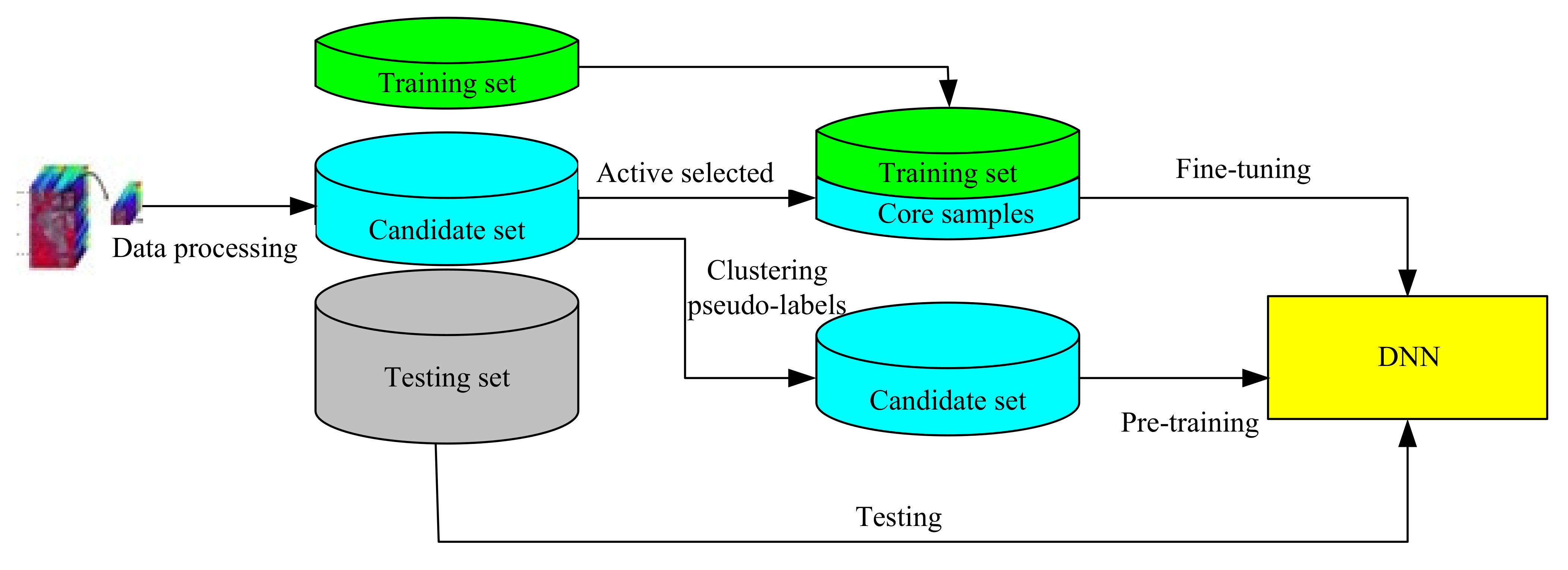
2. The Proposed Method

The cluster inspired active learning method includes four major steps: (1) data pre-processing, which extracts the spectral information of each pixel as the sample and divides all the samples into the training set, candidate set and the testing set; (2) actively selecting core samples from the candidate set via MCFSFDP—the effective MCFSFDP clustering method is utilized to actively select core samples from unlabeled samples in the candidate set for manually labeling; (3) the K-means clustering-based pseudo-labeling scheme is utilized to pre-train the DNN model with samples in candidate set; and (4) fine-tuning and testing, using core samples and small samples as new augmented training samples to fine-tune the network and obtain the final classification result of the testing samples. The flowchart of our proposed method is shown in Figure 1.

2.1. Data Pre-Processing

In this paper, the HSI used in the classification task is denoted as R . An HSI consists of 3D data; we only use the spectral information of each pixel as the sample. We randomly select M pixels from R as limited training samples; in other words, the quantity of the small sample is denoted by M. These selected training samples include all the categories, and each category has almost the same number of pixels. The pixel P i includes the corresponding spectral information with a size of h × 1 as the training sample. h denotes the spectral number of R . { P i } i = 1 M denotes the limited samples, and the limited samples have these manually labeled labels.
Then, we extract N pixels from R and their corresponding spectral information { C j } j = 1 N as unlabeled samples in the candidate set, N denotes the number of samples in the candidate set, i.e., the number of the candidate samples.
Finally, the rest samples are testing samples. K denotes the number of testing samples. { Q u } u = 1 K denotes the testing samples. The samples are also denoted as column vectors, with sizes of h × 1 mathematically.
The samples in the testing set are all used for testing. The core samples are actively selected for labeling via the active learning method, which are selected from the candidate samples. In addition, the K-means clustering method will automatically give the samples in candidate set pseudo-labels for the network pre-training. Here, M plus N is almost equal to K. The samples in the training set, the candidate set and the testing set are not overlapping.
The sample is extracted from R is shown in Figure 2.

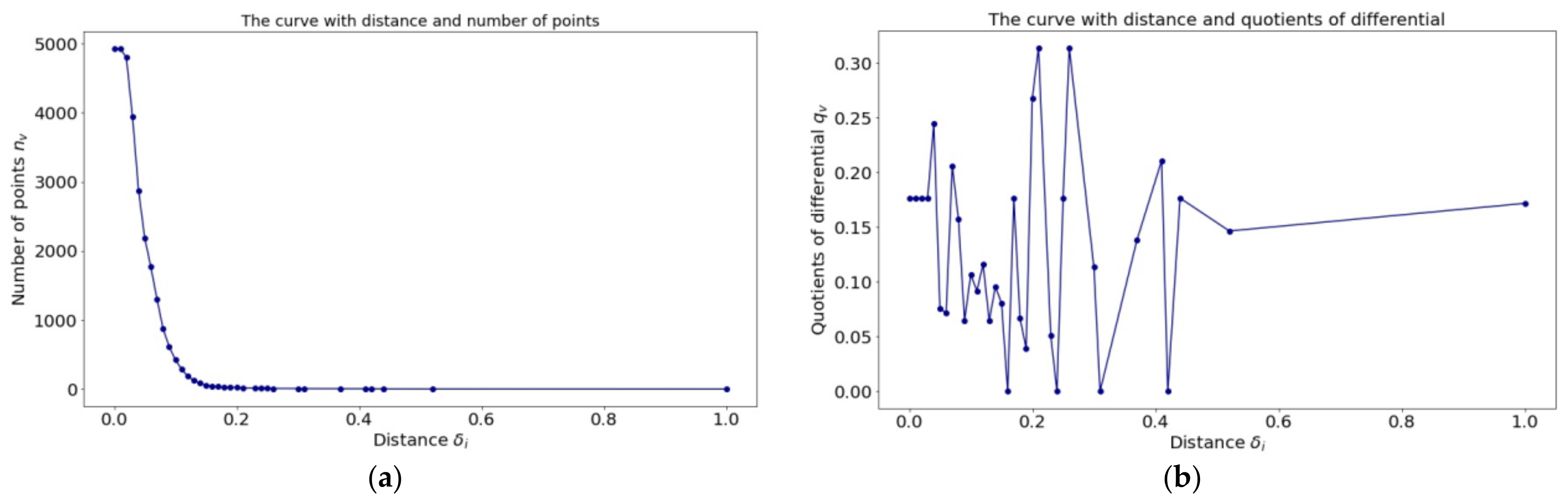
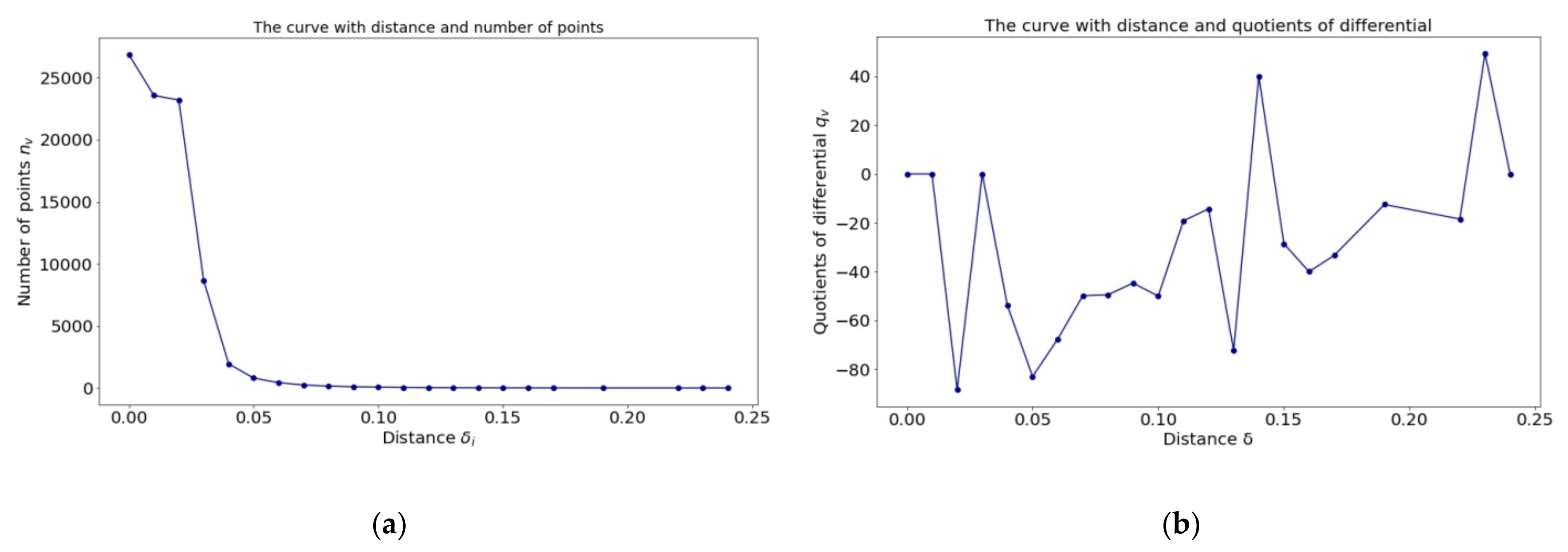
2.2. Actively Selecting Core Samples via MCFSFDP

To actively select the core samples for manually labeling from unlabeled candidate samples, the clustering-based method may be suitable. In our opinion, clustering by fast search and find of peaks (CFSFDP) [43] is a representative method. The idea of this method is that “the cluster centers are determined as those points that not only have higher density than their neighbors, but also keep a certain distance from the point with higher density than them”. In this clustering method, the two thresholds, i.e., distance and density, are important to determine the cluster centers. The points which have higher distances and densities at the same time can be determined as the cluster centers.
In our opinion, CFSFDP is useful in actively selecting the cluster centers and clustering process; however, the wild points (i.e., the inter-class points) are important and difficult to distinguish. To solve this problem, the effective clustering method based on modified clustering by fast search and find of peaks (MCFSFDP), is proposed to actively select core samples by choosing the adaptive distance threshold [28]. The MCFSFDP algorithm is similar to the CFSFDP algorithm in [43], the class center must have two characters, the first character is “a higher density than their neighbors” and the second is “a relatively large distance from points with higher densities”. Different from the CFSFDP, the MCFSFDP chooses the class centers only by larger distance, which can effectively acquire the cluster centers and the wild points and enhance the quality of the selected samples. The details of the proposed method are as follows.
The samples { C j } j = 1 N in candidate set are used for actively selected core samples via clustering based active learning method; for simplicity, each sample C j in candidate set is denoted as point j, which is actually a column vector. For each point j, we calculate the local density ρ j and distance δ j from the point with higher density; if point j has the highest density, the largest distance between j and the other points is denoted as δ j .
The local density ρ j of point j is given in Formula (1):
ρ j = k χ ( d j k d c )
Formula (1) represents the number of samples around the point j in a threshold radius d c . The values of δ j and ρ j are depended on the Euclidean distance d j k , d j k is determined by any pair of the point j and point k. Where χ ( d j k d c ) = 1 if d j k d c < 0 , otherwise, χ ( d j k d c ) = 0 , here, d c is considered as a cut-off distance. ρ j denotes the number of points which in the radius d c and j is the center point.
δ j is the minimum distance between j and any other points with higher density, which is shown in Formula (2):
δ j = min k : ρ k > ρ j ( d j k )
where ρ k denotes the local density of k . For the point with maximum local density, we usually take δ j = max k ( d j k ) . δ j is much larger than the typical nearest neighbor distance only for points that are local or global maxima in the density. The cluster centers are recognized as points for which the value of δ j is anomalously large and the value of ρ j is higher than a value density at the same time.
The distance and density of each point are directly shown in the decision graph. We provided the decision graph of samples in candidate set with a size of 200 × 1 for the Indian Pines dataset [44], as shown in Figure 3. The Indian Pines dataset is often used in the hyperspectral image classification task, which was gathered by AVIRIS sensor over the Indian Pines test site in North-western Indiana and consists of 145 × 145 pixels and 224 spectral reflectance bands in the wavelength range 0.4–2.5 µm.
In the threshold determining step, the MCFSFDP is different from CFSFDP [43], the MCFSFDP is used to select core samples for manually labeling. The distance δ is considered as the only threshold from the decision graph to select samples. This operation can select not only the cluster centers but also the wild points to enhance the quality of samples for increasing the classification result. Because the wild points are in the boundary of any pair of two clusters, which are usually difficult to distinguish, training this type of sample is useful for improving the classification result.
For selecting the core samples adaptively, we should select an optimal distance threshold value δ A .
n v = f ( δ v )
In Formula (3), δ v denotes the distance, which contains points, and f ( δ v ) denotes the mapping relationship of the number n v of points whose distances are larger than or equal to δ v , as shown in Figure 4a.
c v = [ n v + 1 n v ] / ( δ v + 1 δ v )
In Formula (4), where δ v + 1 δ v , c v denotes the differential of n v . Formula (5) denotes the variation quantity of the number points with δ v , as shown in Figure 4b. Formula (4) is the intermediate result of Formulas (3) and (5).
q v = | c v / c v + 1 |
In the MCFSFDP method, the adaptive distance threshold is denoted as δ A , and the points whose distance are larger than δ A are automatically selected as core samples. δ v is an important point that must ensure that the number n v and n v + 1 of points are stable, and at the same time, that the value q v is larger than the value q v + 1 . At this point, δ v is selected as the adaptive distance δ A .
In the Indian Pines dataset, as can be seen from Figure 4a, we can find the distance range (0.15–0.17), and the n v begins to approach stability. As can be seen from Figure 4b, c v with the distance value δ v in range (0.15–0.17) has a local maxima of 0.15. Therefore, 0.15 is considered as the adaptive distance δ A in the Indian Pines dataset.
With the adaptive distance δ A , the points j with the distance value δ j > δ A are adaptively chosen as core samples for manual labeling.
Then, the labeled core samples are added into training samples to form the augmented training set. The number of core samples is denoted as T , and the number of training samples after expansion is M + T . B g g = 1 M + T denotes the final training dataset.

2.3. K-Means Clustering-Based Pseudo-Labeling Scheme

After selecting the core samples via MCFSFDP, we use K-means clustering to obtain the pseudo-labels of the samples C j j = 1 N in candidate set. The steps are as follows:
Step 1: Randomly selecting k samples from C j j = 1 N as the initial cluster centers, i.e., μ 1 , , μ f , , μ k .
Step 2: Calculating the distance between each vector C j with each class center μ f , and the distance is Euclidean distance. If C j is closest to μ f , C j is classified as the category of cluster center μ f .
l a b e l C j = arg min 1 f k C j μ f 2
Step 3: For all c f samples C j , which have the same label of μ f in class f, recalculating the new cluster center through calculating the average value μ f .
μ f = 1 c f j c f C j
where c f is the number of samples in class f .
Step 4: Repeating step 2 and step 3 Z times. Z is the iteration times of the K-means process, which is a parameter. After the computing process, the cluster centers represent the final average values, i.e., μ 1 Z , , μ f Z , , μ k Z . The labels of samples C j j = 1 N in candidate set belong to {1, …, f, …, k}, which are all pseudo-labels by K-means clustering.
The candidate samples with pseudo-labels are utilized to pre-train the DNN model.

2.4. Fine-Tuning and Testing

After obtaining the core samples via MCFSFDP and generating the pseudo-labels of samples C j j = 1 N in candidate set, transfer learning is utilized to train the DNN model. The samples in candidate set with pseudo-labels are utilized to pre-train the DNN model.
Then, the samples B g g = 1 M + T in augmented training set are used to fine-tune the DNN model for obtaining the final network classification model.
Finally, testing the network with the samples Q u u = 1 K in the testing set is performed.
The schematic diagram of the structure of the DNN model and training process is shown in Figure 5. We use the back-propagation neural network [45] as the DNN model. This DNN model contains an input layer, three fully connected layers and a soft-max layer. The first fully connected layer has 512 hidden nodes, the second fully connected layer has 2048 hidden nodes and the third fully connected layer has 1024 hidden nodes. The number of nodes in the soft-max layer varies with the pre-training process and the fine-tuning process because the number of categories with pseudo-labels in candidate set in the pre-training process is different from the number of categories with true labels in the augmented training set in the fine-tuning process.

3. Experiments and Analysis
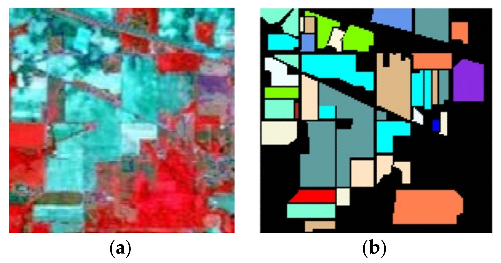
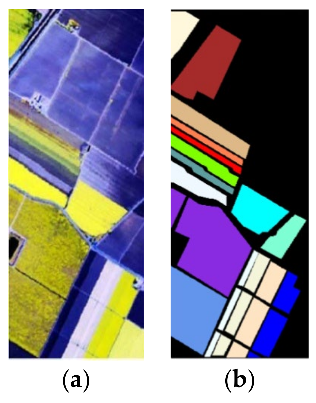
To validate the feasibility and effectiveness of the proposed method, two HSI datasets were used in the experiments. In this section, we firstly introduce the datasets. Secondly, the experimental parameter settings are illustrated. Finally, ablation experiments and comparative experiments are performed to show the HSI classification results of the proposed method.

3.1. Datasets

In this paper, two widely used public HSI image datasets were adopted in our experiments.
Dataset 1: In order to evaluate the proposed method, the first dataset was the Indian Pines image, which was imaged by the Airborne Visual Infrared Imaging Spectrometer (AVIRIS) [44], as shown in Figure 6a. The ground truth is shown in Figure 6b. The size of this image is 145 × 145 pixels with 224 spectral bands, and the wavelength ranges from 0.4 to 2.5 µm. Among the pixels, only 10,249 pixels are feature pixels, and the remaining 10,776 pixels are background pixels. For the exact purpose of eliminating the bands that cannot be reflected by water, the number of bands was reduced to 200. In the actual classification, since background pixels need to be eliminated, there were 16 categories in total. Each category of image samples number is given in Table 1.
The samples in training set could be regarded as limited samples with labels. The samples in candidate set were used for choosing core samples, and the core samples are added into the training samples as a new augmented training set. The samples in candidate set were also used for pre-training the DNNs with their pseudo-labels. The samples in testing set were used for evaluating the effect of the proposed method.
Dataset 2: The second dataset was the Salinas image [44], which was imaged in Salinas Valley in California through AVIRIS as well, as shown in Figure 7a. The ground truth is shown in Figure 7b. Differing from the Indian Pines image, whose spatial resolution is 20 m, its spatial resolution reached 3.7 m. As shown in Figure 6, the size of this image is 512 × 217 pixels, with 224 spectral bands. The number of bands was reduced to 204 after eliminating the low signal-to-noise-ratio (SNR) bands. Among them, 54,129 samples were used for training and testing in total. The details of each category of samples are given in Table 2. This dataset was used to test the feasibility and effectiveness of the proposed approach for classification.

3.2. Experimental Parameter Settings

In the experiment, the samples were randomly selected from the HSI dataset. The training sample set includes 200 samples. For utilizing the effective cluster-inspired active learning method, the samples in candidate set were used to obtain the core samples through the MCFSFDP algorithm for manual labeling, and the pseudo-labels of the samples in candidate set were generated through the K-means algorithm for the DNN’s pre-training. The number of cluster centers was set to 10, 20, …, 100.
In the experiment, as shown in Figure 5, the DNN framework used three fully connected layers and one soft-max layer. In our algorithm, three fully connected layers, namely, hidden layers, all adopted Leaky ReLU as the activation function. The number of neuron nodes in the three hidden layers was 512, 2048 and 1024, respectively. The learning rate was 0.0001. The batch size was designed as 256.
The code was run on a computer with Intel i9-11900K, NVIDIA 3060 GPU × 2, 128 GB Memory, and 1TB SSD.

3.3. Experimental Results

3.3.1. Effectiveness of the Core Samples Actively Selected via MCFSFDP

The effectiveness of the core samples generated by the actively selected method is worthy to be verified. To verify the influence of core samples selected based active learning method in classification, we compared the accuracy of randomly selected samples based active learning method with the accuracy of actively selected core sample-based method, the number of randomly selected samples from candidate set being same as the core samples. The testing accuracy via the training samples with randomly selected samples and training samples with core samples via our proposed MCFSFDP in Dataset 1 is shown in Table 3. Additionally, the testing accuracy for Dataset 2 is shown in Table 4.
In the Indian Pines dataset, the adaptive distance threshold is calculated as 0.15, and we obtain 55 core samples via the MCFSFDP algorithm. The curve for determining the adaptive distance is shown in Figure 4. The adaptive distance is 0.12, and the number of core samples is 40 in Dataset 2. The curve for determining the adaptive distance is shown in Figure 8.
As can be seen from Table 3 and Table 4, the testing result for small samples with core samples is higher than the result for small samples with randomly selected samples. Specifically in Table 4, the overall accuracy (OA) of small samples with core samples is shown to be more than 2% greater than the overall accuracy (OA) of randomly selected samples. Therefore, using the actively selected core samples via MCFSFDP to train the BP neural network can enhance the testing accuracy of the small sample HSI classification. Additionally, the actively selected core sample-based method not only enhances the quantity but also the quality of the training samples.
The other testing results in the two datasets, i.e., the accuracy of each class, average accuracy (AA) and Kappa, which are also shown in Table 3 and Table 4.

3.3.2. Effectiveness of the Proposed Method-Based on Actively Selected Core Samples

Through the above experiments, we have demonstrated the effectiveness of the actively selected core samples method in small sample HSI classification. The classification results prove the effectiveness of the proposed method based on actively selected samples on two datasets.
In the two datasets, the original training samples set, which has 200 samples with their labels, is used for training the BP neural network, while the testing samples set is used for testing the network. In the Indian Pines dataset, the adaptive distance threshold is calculated as 0.15, and we obtain 55 core samples via the MCFSFDP algorithm. These core samples are added into the training samples set and we utilize the new augmented training dataset to train the network. The testing result of the original training samples set and the augmented training samples set with core samples in Dataset 1 is shown in Table 5, while the curve for determining the adaptive distance is shown in Figure 4.
The testing accuracy for the Salinas dataset is shown in Table 6, and the curve for determining the adaptive distance is shown in Figure 8. The adaptive distance is 0.12, and the number of core samples is 40 in dataset 2, which can also be seen in Table 3 and Table 4.
In Table 5, the testing accuracy (OA) with the original training samples set for Dataset 1 is 58.9% after 13,000 training epochs. In contrast to this, the testing accuracy (OA) with the augmented training samples set with core samples in Dataset 1 is 67.8% after 13,000 training epochs. According to the data, the testing accuracy (OA) with the original training samples set is lower than the testing accuracy with the augmented training samples set with core samples.
Additionally, in Table 6, the maximal testing accuracy (OA) with the original training samples set in Dataset 2 is 81.7% after 11,000 training epochs. In contrast to this, the testing accuracy (OA) with the augmented training samples set with core samples for Dataset 2 is 85.6% after 11,000 training epochs. According to the data, the testing accuracy (OA) with the original training samples set is also lower than the testing accuracy (OA) with the training samples set with core samples. Consequently, obtaining the core samples via MCFSFDP added to the training samples set, which is demonstrated to enhance the small sample HSI classification accuracy in Dataset 1 and Dataset 2.
The other testing results in the two datasets, i.e., the accuracy of each class, average accuracy (AA) and Kappa, which are also shown in Table 5 and Table 6.

3.3.3. Effectiveness of Pre-Training by Testing Samples with Pseudo-Labels

Through the above experiments, we have proved the effectiveness of active learning in small sample HSI classification. In order to demonstrate the effectiveness of the proposed method of pre-training using candidate samples with pseudo-labels via clustering combined with adaptive active learning, we labeled the pseudo-labels for the candidate samples via the K-means algorithm and utilized these data to pre-train the BP neural network. Then, the training samples set with core samples is used for fine-tuning the network.
To determine the appropriate number of clusters for pseudo-labels, we observe the testing accuracy of the proposed method with a different number of clusters after 13,000 training epochs in Dataset 1. The testing accuracy of the proposed method with different numbers of clusters after 13,000 training epochs in Dataset 1 is shown in Table 7. The testing accuracy of the proposed method with different numbers of clusters after 11,000 training epochs in Dataset 2 is shown in Table 8.
In Table 7, the maximal testing accuracy (68.9%) of the proposed method for Dataset 1 shows that the number of cluster centers is 50 when using 13,000 training epochs. Compared with the value of Table 5, the testing accuracy of the proposed method is higher than that of the original training samples set (58.9%) and the training samples set with core samples 67.8%). According to the data, compared with the method of only adaptive active learning, the testing accuracy of the proposed method significantly improved. Additionally, in Table 8, the maximal testing accuracy (86.8%) of the proposed method for Dataset 2 shows that the number of cluster centers is 80 when using 11,000 training epochs. Compared with the value of Table 6, the testing accuracy of the proposed method is higher than that of the original training samples set (81.7%) and the training samples set with core samples (85.6%).
In Table 7 and Table 8, due to the different distributions of samples in the two datasets, the number of clusters in the Indian Pines dataset and the Salinas dataset are different, which choose 50 clusters and 80 clusters, respectively. Consequently, the proposed cluster-inspired active learning method is demonstrated to enhance the small sample HSI classification accuracy and has a better effect than the above method in Table 3, Table 4, Table 5 and Table 6 on Dataset 1 and Dataset 2.

3.3.4. The Proposed Method Compared with the Other Methods

In these experiments, our method is compared with other methods, including random based active learning method, K-means based active learning method, minimum probability-based active learning method, CFSFDP based active learning method [43] and our MCFSFDP based active learning method [28] and the proposed cluster inspired active learning method.
Specifically speaking, K-means selected sample-based method utilizes the K-means algorithm to extracts samples. Minimum probability-based active learning method uses n minimum probabilities of predicted samples to choose samples. CFSFDP and MCFSFDP selected sample-based methods are used to increase the number of samples. The classification effect is different through Back-Propagation neural network. The testing accuracy (OA) of these methods compared with the proposed method for Dataset 1 is shown in Table 9. The testing accuracy (OA) for Dataset 2 is shown in Table 10.
Through the classification results of different methods for Dataset 1 and 2, it can be seen that the testing accuracy of the proposed cluster-inspired active learning method is better than the other methods. Among them, the testing accuracy of K-means-based active learning method is lowest, and our MCFSFDP based active learning method is the second-best method.

4. Discussion

4.1. Influence of the Network Training Iterations

The experimental results in Table 11 and Table 12 show that adding the core samples into the training samples set for training the network can obtain better testing accuracy than using original small samples for Dataset 1 and Dataset 2.
According to the data in Table 11, the number of epochs, which is 13,000, is confirmed as the best training iteration with core samples, as it obtains the testing accuracy (58.9%) in the original training samples set for Dataset 1. The testing accuracy of the training samples set with core samples is 67.8%, which is the best testing accuracy of training samples with core samples, subsequent experiments still use 13,000 epochs as the best training iteration. The best testing accuracy in the original training sample set is 60.1% with the 11,000 iterations. In addition, we choose 13,000 epochs as the iteration times in Dataset 1. The iteration influence curve is shown in Figure 9.
According to the data in Table 12, the number of epochs, which is 6000, is confirmed as the best training period for attaining the best testing accuracy (82.9%) in the original training samples set for Dataset 2. The testing accuracy of the training samples set with core samples is 84.1%, which is higher than that of the original samples set. However, the testing accuracy of training samples with core samples trained using 11,000 epochs is 85.6%, it is the best training result, and subsequent experiments use 11,000 epochs as the condition. The iteration influence curve is shown in Figure 10.

4.2. Influence of the Number of Clusters and Iterations

As can be seen from Table 13 and Table 14, the testing accuracy of the proposed method is influenced by the number of clusters via K-means and the network training epochs.
In Table 13, the best accuracy is shown to be 68.9%, when we choose 13,000 iterations and 50 clusters for Dataset 1. The best testing accuracy, as shown in Table 14, is 86.8% with the best parameters, which are 11,000 iterations and 80 clusters. Therefore, Table 9 and Table 10 demonstrate the two best accuracies as the final results for Dataset 1 and Dataset 2.

5. Conclusions

In this paper, we present a cluster-inspired active learning method for HSI classification, which mainly contributes to two aspects. On one hand, the modified clustering by fast search and find of peaks (MCFSFDP) clustering method is utilized to select highly informative and diverse samples from samples in candidate set for manual labeling, which empowers us to appropriately augment the limited training set (i.e., labeled samples) and thus improve the generalization capacity of the baseline DNNs model. On the other hand, another K-means clustering-based pseudo-labeling scheme is utilized to pre-train the DNN model with all samples candidate set. By doing this, the pre-trained model can be effectively generalized to testing samples after being fine-tuned based on the augmented training set. The experimental results demonstrate that the proposed method is useful in selecting core samples with high quality to expand the data and improve the small sample HSI classification accuracy effectively.

Author Contributions

Conceptualization, C.D. and L.Z.; methodology, C.D., L.Z. and W.W.; validation, Y.Z. (Yuankun Zhang), F.C., X.Z., E.F. and D.W.; formal analysis, L.Z. and W.W.; investigation, M.Z. and F.C.; resources, C.D. and D.W.; data curation, C.D. and M.Z.; writing—original draft preparation, C.D. and M.Z.; writing—review and editing, C.D., Y.Z. (Yanning Zhang), L.Z. and W.W.; supervision, Y.Z. (Yanning Zhang), W.W. and L.Z.; project administration, Y.Z. (Yuankun Zhang) and F.C.; funding acquisition, C.D., W.W. and L.Z. All authors have read and agreed to the published version of the manuscript.

Funding

This work was supported by the National Natural Science Foundations of China (grant no.61901369, grant no.62071387 and grant no.62101454), the Foundation of National Engineering Laboratory for Integrated Aero-Space-Ground- Ocean Big Data Application Technology (grant no.20200203) and the National Key Research and Development Project of China (No. 2020AAA0104603).

Data Availability Statement

Not applicable.

Acknowledgments

We acknowledge AVIRIS sensor for gathering the Indian Pines test site in North-western Indian and Salinas Valley, California.

Conflicts of Interest

The authors declare no conflict of interest.

References

  1. Landgrebe, D. Hyperspectral image data analysis. IEEE Signal Process. Mag. 2002, 19, 17–28. [Google Scholar] [CrossRef]
  2. Shaw, G.; Manolakis, D. Signal processing for hyperspectral image exploitation. IEEE Signal Process. Mag. 2002, 19, 12–16. [Google Scholar] [CrossRef]
  3. Myasnikov, E.V. Hyperspectral image segmentation using dimensionality reduction and classical segmentation approaches. Samara Natl. Res. 2017, 41, 564–572. [Google Scholar] [CrossRef]
  4. Andriyanov, N.; Dementiev, V.; Gladkikh, A. Analysis of the Pattern Recognition Efficiency on Non-Optical Images. In Proceedings of the 2021 Ural Symposium on Biomedical Engineering, Radioelectronics and Information Technology (USBEREIT), Yekaterinburg, Russia, 13–14 May 2021; pp. 0319–0323. [Google Scholar]
  5. Lazcano, R.; Madronal, D.; Florimbi, G.; Sancho, J.; Sanchez, S.; Leon, R.; Fabelo, H.; Ortega, S.; Torti, E.; Salvador, R.; et al. Parallel Implementations Assessment of a Spatial-Spectral Classifier for Hyperspectral Clinical Applications. IEEE Access 2019, 7, 152316–152333. [Google Scholar] [CrossRef]
  6. Eismann, M.T.; Hardie, R.C. Application of the stochastic mixing model to hyperspectral resolution enhancement. IEEE Trans. Geosci. Remote Sens. 2004, 42, 1924–1933. [Google Scholar] [CrossRef]
  7. Chang, C.-I. An information-theoretic approach to spectral variability, similarity, and discrimination for hyperspectral image analysis. IEEE Trans. Inf. Theory 2000, 46, 1927–1932. [Google Scholar] [CrossRef] [Green Version]
  8. Jia, X.; Richards, J.A. Efficient maximum likelihood classification for imaging spectrometer data sets. IEEE Trans. Geosci. Remote Sens. 1994, 32, 274–281. [Google Scholar]
  9. Chen, S.; Gunn, S.R.; Harris, C.J. The relevance vector machine technique for channel equalization application. IEEE Trans. Neural Netw. 2001, 12, 1529–1532. [Google Scholar] [CrossRef]
  10. Li, J.; Bioucas-Dias, J.M.; Plaza, A. Semisupervised Hyperspectral Image Segmentation Using Multinomial Logistic Regression with Active Learning. IEEE Trans. Geosci. Remote Sens. 2010, 48, 4085–4098. [Google Scholar] [CrossRef] [Green Version]
  11. Chen, Y.; Nasrabadi, N.M.; Tran, T.D. Hyperspectral Image Classification via Kernel Sparse Representation. IEEE Trans. Geosci. Remote Sens. 2013, 51, 217–231. [Google Scholar] [CrossRef] [Green Version]
  12. Melgani, F.; Bruzzone, L. Classification of hyperspectral remote sensing images with support vector machines. IEEE Trans. Geosci. Remote Sens. 2004, 42, 1778–1790. [Google Scholar] [CrossRef] [Green Version]
  13. Fang, L.; Li, S.; Kang, X.; Benediktsson, J.A. Spectral–Spatial Hyperspectral Image Classification via Multiscale Adaptive Sparse Representation. IEEE Trans. Geosci. Remote Sens. 2014, 52, 7738–7749. [Google Scholar] [CrossRef]
  14. Baassou, B.; He, M.; Mei, S.; Zhang, Y. Unsupervised hyperspectral image classification algorithm by integrating spatial-spectral information. In Proceedings of the 2012 International Conference on Audio, Language and Image Processing, Shanghai, China, 16–18 July 2012; pp. 610–615. [Google Scholar]
  15. Lary, D.J.; Alavi, A.H.; Gandomi, A.H.; Walker, A.L. Machine learning in geosciences and remote sensing. Geosci. Front. 2016, 7, 3–10. [Google Scholar] [CrossRef] [Green Version]
  16. Chen, L.; Wei, Z.; Xu, Y. A Lightweight Spectral–Spatial Feature Extraction and Fusion Network for Hyperspectral Image Classification. Remote Sens. 2020, 12, 1395. [Google Scholar] [CrossRef]
  17. Ma, W.; Ma, H.; Zhu, H.; Li, Y.; Li, L.; Jiao, L.; Hou, B. Hyperspectral Image Classification Based on Spatial and Spectral Kernels Generation Network. Inf. Sci. 2021, 578, 435–456. [Google Scholar] [CrossRef]
  18. Hang, R.; Li, Z.; Liu, Q.; Ghamisi, P.; Bhattacharyya, S.S. Hyperspectral image classification with attention aided CNNs. IEEE Trans. Geosci. Remote Sens. 2020, 59, 2281–2293. [Google Scholar] [CrossRef]
  19. Abdulsamad, T.; Chen, F.; Xue, Y.; Wang, Y.; Zeng, D. Hyperspectral image classification based on spectral and spatial information using resnet with channel attention. Opt. Quantum Electron. 2021, 53, 1–20. [Google Scholar] [CrossRef]
  20. Pande, S.; Banerjee, B. Adaptive hybrid attention network for hyperspectral image classification. Pattern Recognit. Lett. 2021, 144, 6–12. [Google Scholar] [CrossRef]
  21. Zhu, M.; Jiao, L.; Liu, F.; Yang, S.; Wang, J. Residual spectral-spatial attention network for hyperspectral image classification. IEEE Trans. Geosci. Remote Sens. 2020, 59, 449–462. [Google Scholar] [CrossRef]
  22. Chen, Y.; Lin, Z.; Zhao, X.; Wang, G.; Gu, Y. Deep Learning-Based Classification of Hyperspectral Data. IEEE J. Sel. Top. Appl. Earth Obs. Remote Sens. 2014, 7, 2094–2107. [Google Scholar] [CrossRef]
  23. Chen, Y.; Zhao, X.; Jia, X. Spectral–Spatial Classification of Hyperspectral Data Based on Deep Belief Network. IEEE J. Sel. Top. Appl. Earth Obs. Remote Sens. 2015, 8, 2381–2392. [Google Scholar] [CrossRef]
  24. Hu, W.; Huang, Y.; Wei, L.; Zhang, F.; Li, H. Deep Convolutional Neural Networks for Hyperspectral Image Classification. J. Sens. 2015, 2015, 258619. [Google Scholar] [CrossRef] [Green Version]
  25. Yang, J.; Zhao, Y.; Chan, J.C.-W.; Yi, C. Hyperspectral image classification using two-channel deep convolutional neural network. In Proceedings of the 2016 IEEE International Geoscience and Remote Sensing Symposium (IGARSS), Beijing, China, 10–15 July 2016; pp. 5079–5082. [Google Scholar]
  26. Chen, Y.; Jiang, H.; Li, C.; Jia, X.; Ghamisi, P. Deep feature extraction and classification of hyperspectral images based on convolutional neural networks. IEEE Trans. Geosci. Remote Sens. 2016, 54, 6232–6251. [Google Scholar] [CrossRef] [Green Version]
  27. Chan, T.-H.; Jia, K.; Gao, S.; Lu, J.; Zeng, Z.; Ma, Y. PCANet: A Simple Deep Learning Baseline for Image Classification? IEEE Trans. Image Process. 2015, 24, 5017–5032. [Google Scholar] [CrossRef] [PubMed] [Green Version]
  28. Ding, C.; Li, Y.; Xia, Y.; Wei, W.; Zhang, L.; Zhang, Y. Convolutional Neural Networks Based Hyperspectral Image Classification Method with Adaptive Kernels. Remote Sens. 2017, 9, 618. [Google Scholar] [CrossRef] [Green Version]
  29. Fahad, A.; Alshatri, N.; Tari, Z.; Alamri, A.; Khalil, I.; Zomaya, A.Y.; Foufou, S.; Bouras, A. A Survey of Clustering Algorithms for Big Data: Taxonomy and Empirical Analysis. IEEE Trans. Emerg. Top. Comput. 2014, 2, 267–279. [Google Scholar] [CrossRef]
  30. Zhang, G.; Zhao, S.; Li, W.; Du, Q.; Ran, Q.; Tao, R. HTD-Net: A Deep Convolutional Neural Network for Target Detection in Hyperspectral Imagery. Remote Sens. 2020, 12, 1489. [Google Scholar] [CrossRef]
  31. Wei, Y.; Zhou, Y. Spatial-Aware Network for Hyperspectral Image Classification. Remote Sens. 2021, 13, 3232. [Google Scholar] [CrossRef]
  32. Li, W.; Wu, G.; Zhang, F.; Du, Q. Hyperspectral image classification using deep pixel-pair features. IEEE Trans. Geosci. Remote Sens. 2016, 55, 844–853. [Google Scholar] [CrossRef]
  33. Kemker, R.; Kanan, C. Self-Taught Feature Learning for Hyperspectral Image Classification. IEEE Trans. Geosci. Remote Sens. 2017, 55, 2693–2705. [Google Scholar] [CrossRef]
  34. Zhong, Z.; Li, J.; Luo, Z.; Chapman, M. Spectral-spatial residual network for hyperspectral image classification: A 3-d deep learning framework. IEEE Trans. Geosci. Remote Sens. 2017, 56, 847–858. [Google Scholar] [CrossRef]
  35. Fang, B.; Li, Y.; Zhang, H.; Chan, J.C.-W. Hyperspectral Images Classification Based on Dense Convolutional Networks with Spectral-Wise Attention Mechanism. Remote Sens. 2019, 11, 159. [Google Scholar] [CrossRef] [Green Version]
  36. Paoletti, M.E.; Haut, J.M.; Fernandez-Beltran, R.; Plaza, J.; Plaza, A.; Li, J.; Pla, F. Capsule networks for hyperspectral image classification. IEEE Trans. Geosci. Remote Sens. 2019, 57, 2145–2160. [Google Scholar] [CrossRef]
  37. Li, W.; Wei, W.; Zhang, L.; Wang, C.; Zhang, Y. Unsupervised deep domain adaptation for hyperspectral image classification. In Proceedings of the IEEE International Geoscience and Remote Sensing Symposium, Yokohama, Japan, 28 July–2 August 2019; pp. 1–4. [Google Scholar] [CrossRef]
  38. Wang, W.; Chen, Y.; He, X.; Li, Z. Soft Augmentation-Based Siamese CNN for Hyperspectral Image Classification with Limited Training Samples. IEEE Geosci. Remote Sens. Lett. 2021, 19, 1–5. [Google Scholar] [CrossRef]
  39. Cui, Y.; Yu, Z.; Han, J.; Gao, S.; Wang, L. Dual-Triple Attention Network for Hyperspectral Image Classification Using Limited Training Samples. IEEE Geosci. Remote Sens. Lett. 2021. [Google Scholar] [CrossRef]
  40. Radford, A.; Metz, L.; Chintala, S. Unsupervised Representation Learning with Deep Convolutional Generative Adversarial Networks. In Proceedings of the ICLR 2016: International Conference on Learning Representations, San Juan, PR, USA, 2–4 May 2016. [Google Scholar]
  41. Creswell, A.; White, T.; Dumoulin, V.; Arulkumaran, K.; Sengupta, B.; Bharath, A.A. Generative Adversarial Networks: An Overview. IEEE Signal Process. Mag. 2018, 35, 53–65. [Google Scholar] [CrossRef] [Green Version]
  42. Zhu, L.; Chen, Y.; Ghamisi, P.; Benediktsson, J.A. Generative Adversarial Networks for Hyperspectral Image Classification. IEEE Trans. Geosci. Remote Sens. 2018, 56, 5046–5063. [Google Scholar] [CrossRef]
  43. Rodriguez, A.; Laio, A. Clustering by fast search and find of density peaks. Science 2014, 344, 1492–1496. [Google Scholar] [CrossRef] [Green Version]
  44. Hyperspectral Remote Sensing Scenes. Available online: http://www.ehu.eus/ccwintco/index.php?title=Hyperspectral_Remote_Sensing_Scenes (accessed on 10 December 2021).
  45. Olden, J.D.; Jackson, D.A. Illuminating the “black box”: A randomization approach for understanding variable contributions in artificial neural networks. Ecol. Model. 2002, 154, 135–150. [Google Scholar] [CrossRef]
Figure 1. The flow chart of the proposed method.
Remotesensing 14 00596 g001
Figure 2. The sample is extracted from image R.
Remotesensing 14 00596 g002
Figure 3. Decision graph of samples in candidate set with a size of 200 × 1 for Indian Pines.
Remotesensing 14 00596 g003
Figure 4. The curves for determining the adaptive distance δ A in the candidate set of Indian Pines dataset with sample size of 200 × 1. (a) shows the curve of the point-number over distance δ v ; (b) gives the curve of the quotients of differential over distance δ v .
Remotesensing 14 00596 g004
Figure 5. The schematic diagram of the structure of the DNN model and training process.
Remotesensing 14 00596 g005
Figure 6. The Indian Pines image in Dataset 1. (a) shows the composite image; (b) shows the ground truth of the Indian Pines dataset, where the black area denotes the unlabeled pixels.
Remotesensing 14 00596 g006
Figure 7. The Salinas scene in Dataset 2. (a) shows the composite image; (b) shows the ground truth of the Salinas Dataset, where the black area denotes the unlabeled pixels.
Remotesensing 14 00596 g007
Figure 8. The curve for determining the adaptive distance in the Salinas scene dataset. (a) shows the curve of the point-number over distance δ v ; (b) gives the curve of the quotients of differential over distance δ v .
Remotesensing 14 00596 g008
Figure 9. The classification accuracy with the training epochs for Dataset 1.
Remotesensing 14 00596 g009
Figure 10. The classification accuracy with the training epochs for Dataset 2.
Remotesensing 14 00596 g010
Table 1. Ground truth of classes and number of their respective samples in the Indian Pines scene.
Class Samples
NumberClassesTotalTrainingCandidateTesting
1Alfalfa4661723
2Corn-notill142826688714
3Corn-mintill83012403415
4Corn2377112118
5Grass-pasture4838234241
6Grass-trees73016349365
7Grass-pasture-mowed285914
8Hay-windrowed47813226239
9Oats205510
10Soybean-notill97212474486
11Soybean-mintill24553811901227
12Soybean-clean59311286296
13Wheat205796102
14Woods126515618632
15Building-Grass-Trees38612181193
16Stone-Steel-Towers9374046
Total10,24920049285121
Table 2. Ground truth of classes and number of their respective samples in the Salinas scene.
Class Samples
NumberClassesTotalTrainingCandidateTesting
1Broccoli_green_weeds_12009119941004
2Broccoli_green_weeds_237261618471863
3Fallow197612976988
4Fallow_rough_plow139410687697
5Fallow_smooth26781113281339
6Stubble39591919611979
7Celery35791317771789
8Grapes_untrained11,2711456225635
9Soil_vinyard_develop62031530873101
10Corn_senesced_green_weeds32781016291639
11Lettuce_romaine_4wk106812522534
12Lettuce_romaine_5wk192713951963
13Lettuce_romaine_6wk91610448458
14Lettuce_romaine_7wk107011524535
15Vinyard_untrained72681536213634
16Vinyard_vertical_trellis180710894903
Total54,12920026,86827,061
Table 3. The testing result of randomly selected samples and core samples via MCFSFDP in Dataset 1.
ClassThe Adaptive
Distance
Threshold
The Number of
Selected Core
Samples
Testing Accuracy (%)
Randomly Selected SamplesCore
Samples
10.155539.165.2
251.857.1
347.056.1
441.547.5
578.466.0
694.893.2
771.485.7
895.090.0
920.020.0
1059.552.3
1173.177.0
1232.840.2
13100.099.0
1475.580.1
1535.232.6
1695.789.1
OA (%) 65.967.8
AA (%) 63.265.7
Kappa 61.164.2
Table 4. The testing result of randomly selected samples and core samples via MCFSFDP in Dataset 2.
ClassThe Adaptive
Distance
Threshold
The Number of
Selected Core
Samples
Testing Accuracy (%)
Randomly Selected SamplesCore
Samples
10.124099.095.0
297.099.4
345.166.5
499.799.6
578.394.2
699.699.1
799.298.3
888.282.3
994.596.8
1067.574.6
1191.699.1
1297.097.0
1399.099.0
1490.890.5
1545.855.8
1688.084.6
OA (%) 83.185.6
AA (%) 86.389.5
Kappa 81.384.0
Table 5. The testing result of original training samples set and training samples set with core samples in Dataset 1.
ClassTesting Accuracy (%)
Original Training Samples SetTraining Samples Set with Core Samples
147.865.2
247.357.1
349.656.1
444.147.5
529.966.0
692.693.2
785.785.7
893.390.0
920.020.0
1030.252.3
1169.477.0
1229.440.2
13100.099.0
1474.580.1
1531.132.6
1693.589.1
OA (%)58.967.8
AA (%)58.565.7
Kappa52.864.2
Table 6. The testing result of original training samples set and training samples set with core samples in Dataset 2.
ClassTesting Accuracy (%)
Original Training Samples SetTraining Samples Set with Core Samples
199.195.0
297.599.4
355.966.5
499.799.6
573.094.2
699.699.1
799.298.3
890.182.3
996.096.8
1064.274.6
1194.299.1
1298.497.0
1398.799.0
1490.590.5
1530.055.8
1683.584.6
OA (%)81.785.6
AA (%)56.689.5
Kappa80.084.0
Table 7. The testing accuracy of the proposed method with different numbers of clusters in Dataset 1.
The Number of Clusters102030405060708090100
Testing Accuracy OA (%)63.764.665.366.268.966.165.865.766.566.6
Table 8. The testing accuracy of the proposed method with different numbers of clusters in Dataset 2.
The Number of Clusters102030405060708090100
Testing Accuracy OA (%)85.585.986.085.985.985.885.986.886.185.4
Table 9. The testing accuracy of the proposed method compared with the other methods for Dataset 1.
Dataset 1Testing Accuracy (%)
Random
Selected
Samples
K-Means
Selected
Samples
Minimum
Probability
Selected Samples
CFSFDP
Selected
Samples
MCFSFDP
Selected
Samples
Proposed
Method
OA (%)65.959.663.964.467.868.9
Table 10. The testing accuracy of the proposed method compared with the other methods for Dataset 2.
Dataset 2Testing Accuracy (%)
Random
Selected
Samples
K-Means
Selected
Samples
Minimum
Probability
Selected Samples
CFSFDP
Selected
Samples
MCFSFDP
Selected
Samples
Proposed
Method
OA (%)83.182.983.885.185.686.8
Table 11. The testing accuracy of original training samples set and training samples set with core samples for Dataset 1.
DatasetEpochsTesting Accuracy OA (%)
Original Training SetTraining Set with Core Samples
Indian Pines100056.161.7
200059.264.6
300058.766.1
400059.566.2
500059.766.4
600056.964.8
700059.566.2
800058.866.2
900059.166.6
10,00058.867.6
11,00060.164.9
12,00059.367.6
13,00058.967.8
14,00059.467.7
15,00058.766.9
Table 12. The testing accuracy of original training samples set and training samples set with core samples for Dataset 2.
DatasetEpochsTesting Accuracy OA (%)
Original Training SetTraining Set with Core Samples
Salinas100071.171.8
200079.278.1
300080.681.5
400081.382.8
500082.284.0
600082.984.1
700082.284.7
800082.284.6
900082.485.4
10,00081.485.5
11,00081.785.6
12,00080.985.5
13,00079.685.4
14,00079.185.1
15,00078.585.2
Table 13. The testing accuracy of the proposed method with different numbers of clusters and iterations for Dataset 1.
DatasetThe Number of ClustersTesting Accuracy OA (%)
Epochs102030405060708090100
Indian Pines100060.861.863.364.366.663.862.262.662.663.7
200062.862.763.362.967.065.464.664.464.365.7
300062.463.362.863.668.163.764.765.166.165.7
400061.164.764.265.667.963.764.165.166.266.6
500062.264.664.164.967.764.862.965.466.266.6
600062.562.964.263.267.665.365.165.366.766.3
700063.764.364.464.867.364.865.465.966.867.5
800065.563.464.565.467.866.565.864.965.566.0
900063.262.957.465.667.964.864.964.965.767.9
10,00064.163.465.066.968.164.664.865.764.966.8
11,00063.065.261.963.868.465.965.766.365.967.2
12,00063.464.265.865.868.465.365.165.565.767.3
13,00063.764.665.366.268.966.165.865.766.566.6
14,00063.963.764.866.967.665.964.966.865.167.4
15,00063.464.466.166.868.365.365.264.864.166.8
Table 14. The testing accuracy of the proposed method with different numbers of clusters and iterations for Dataset 2.
DatasetThe Number of ClustersTesting Accuracy OA (%)
Epochs102030405060708090100
Salinas100078.478.278.177.778.677.177.778.277.177.4
200079.979.879.878.980.180.279.780.880.779.4
300080.682.281.379.782.181.780.981.983.680.2
400082.084.282.480.783.783.282.584.384.680.8
500083.485.184.181.984.484.383.785.384.883.1
600084.485.484.582.285.184.984.485.284.983.6
700084.685.685.283.985.585.384.785.885.684.4
800084.985.785.384.285.985.885.286.185.884.8
900085.386.185.784.486.185.785.386.485.985.1
10,00085.686.285.885.186.385.885.486.785.984.8
11,00085.585.986.085.585.985.885.986.886.185.4
12,00085.786.285.585.286.385.686.086.186.285.0
13,00085.385.885.785.386.085.686.386.686.384.5
14,00085.685.585.884.785.985.286.386.485.985.8
15,00085.985.785.784.985.685.386.286.486.586.2
Publisher’s Note: MDPI stays neutral with regard to jurisdictional claims in published maps and institutional affiliations.

