
An Improved Generalized Hierarchical Estimation Framework with Geostatistics for Mapping Forest Parameters and Its Uncertainty: A Case Study of Forest Canopy Height

 ,
,
Abstract
:
1. Introduction
2. Materials and Methods
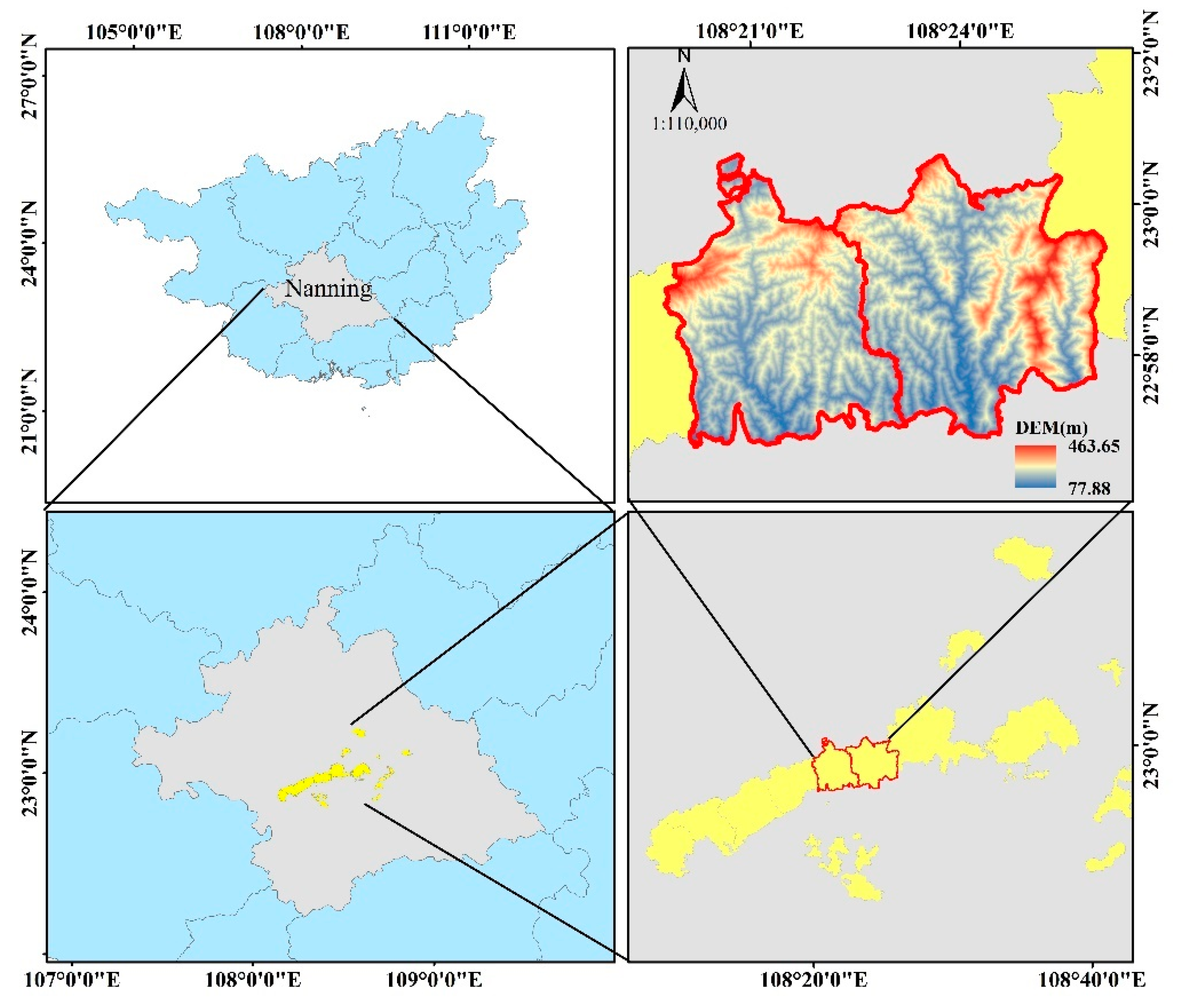
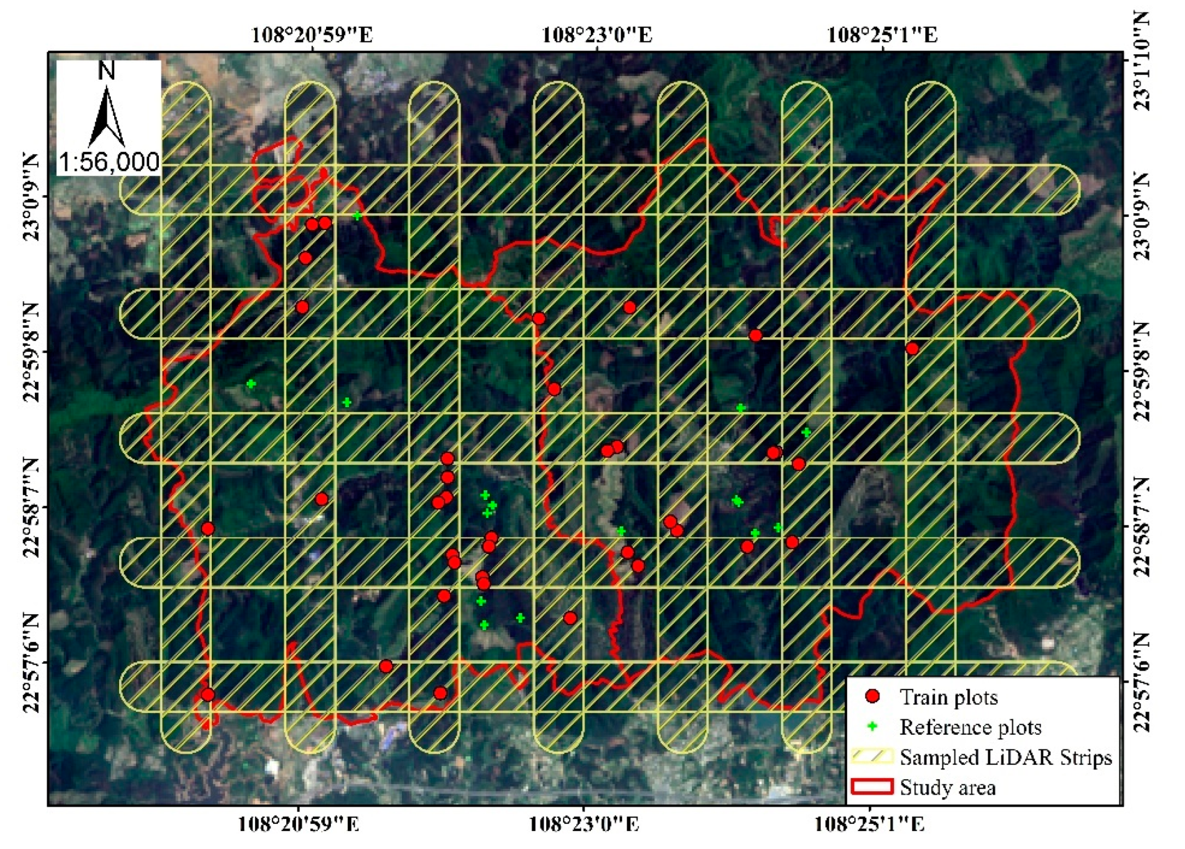
2.1. Study Area
2.2. Data
2.2.1. Plot Data
2.2.2. ALS Data Acquisition and Processing
2.2.3. ZY3 Stereo Images and Processing
2.3. Methods
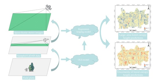
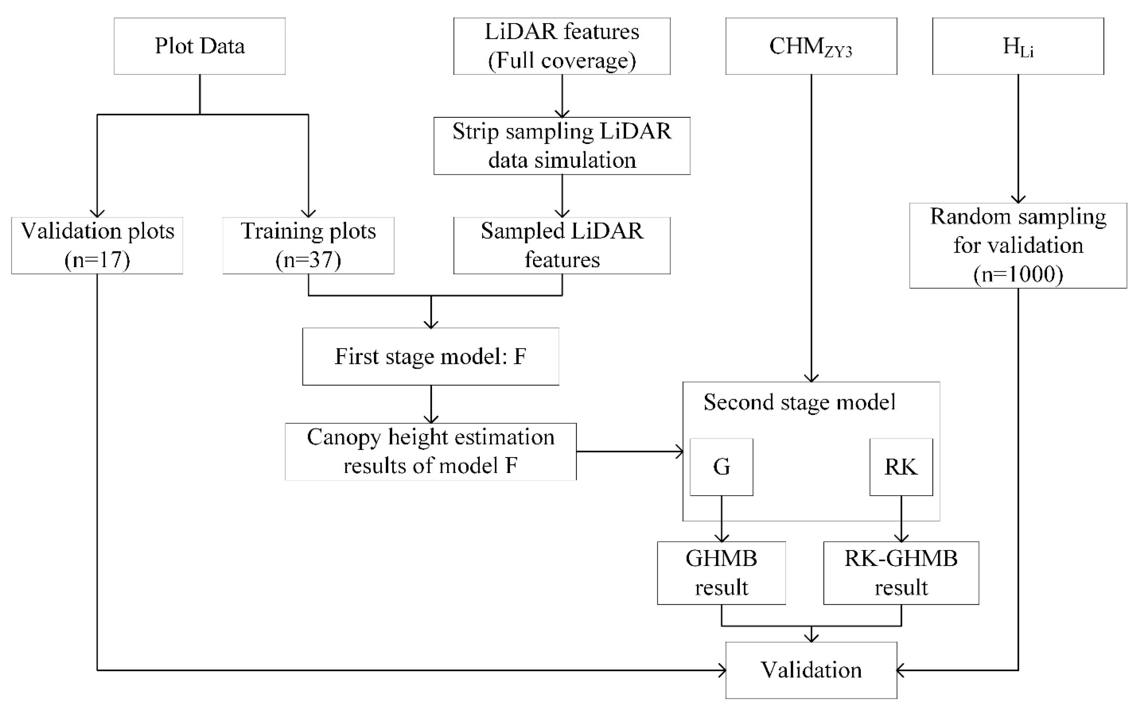
2.3.1. Overview
2.3.2. GHMB
Regression Model
Uncertainties Estimation
2.3.3. RK-GHMB
Regression Model
Uncertainties Estimation
2.3.4. Accuracy Assessment
3. Results
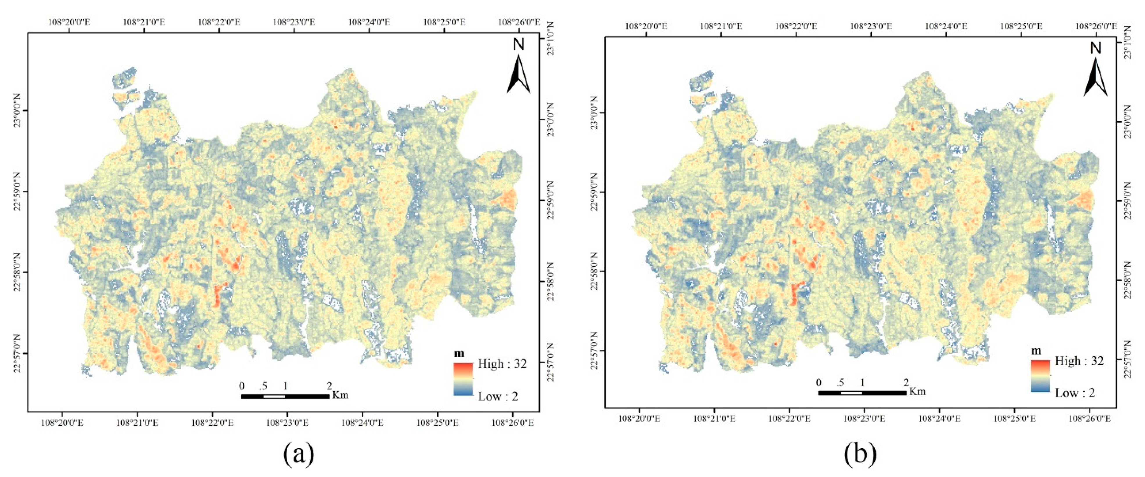
3.1. Forest Canopy Height Estimation Result of GHMB
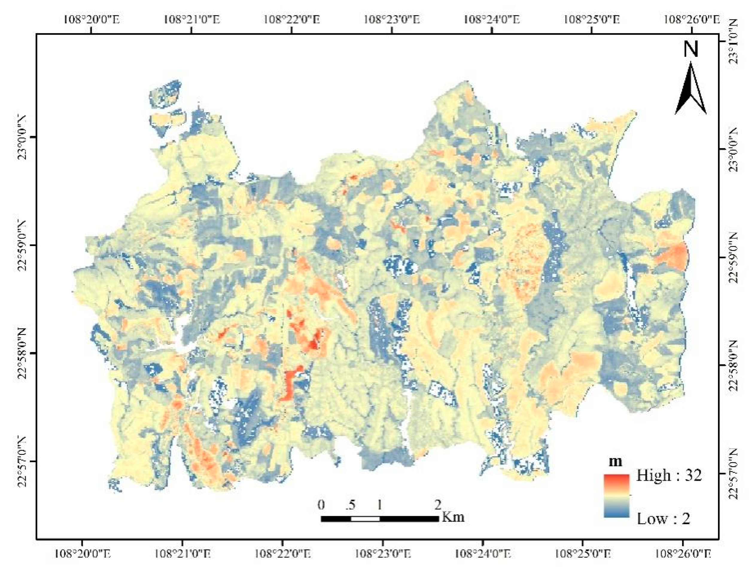
3.2. Forest Canopy Height Estimation Result of RK-GHMB
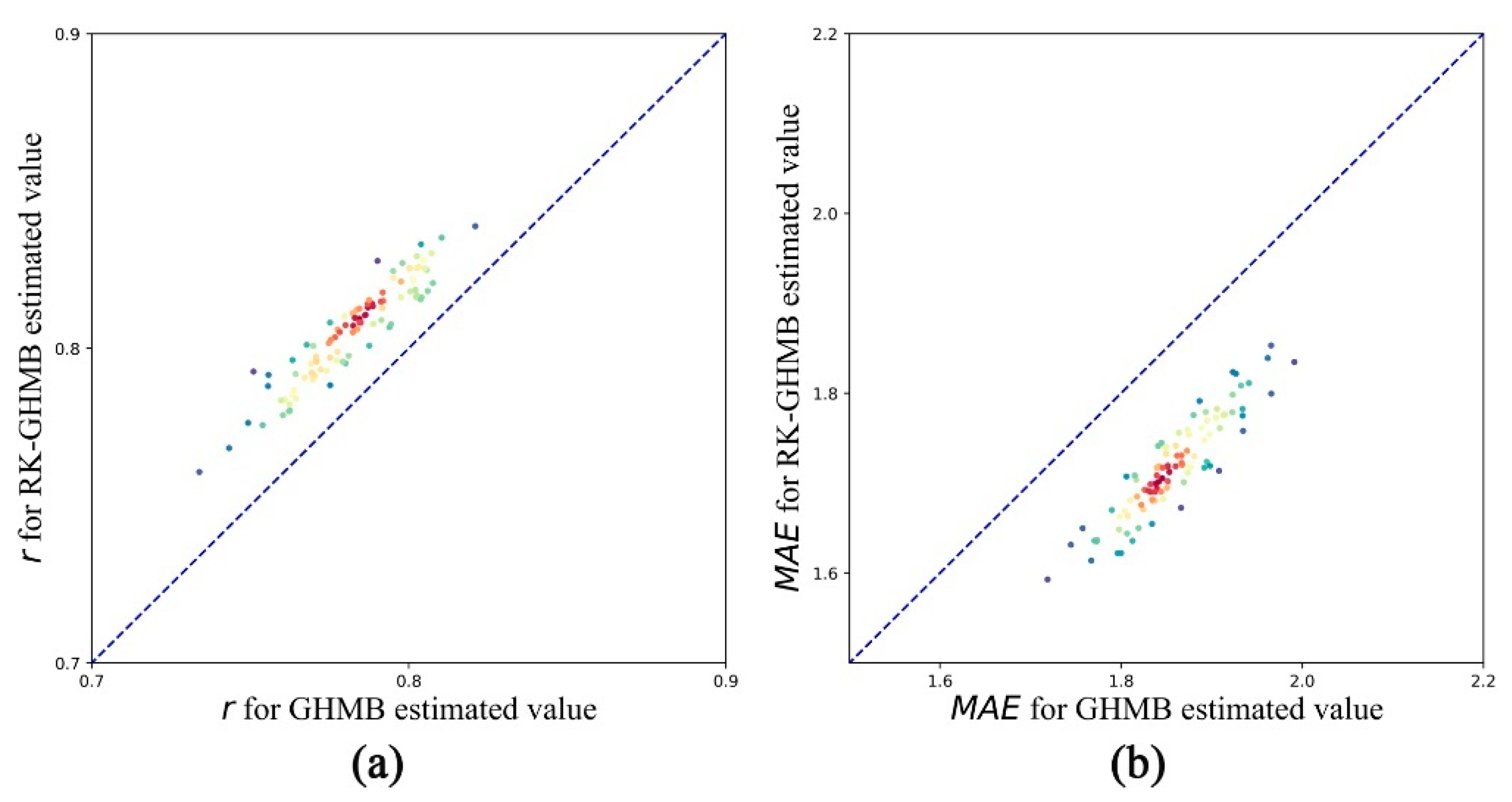
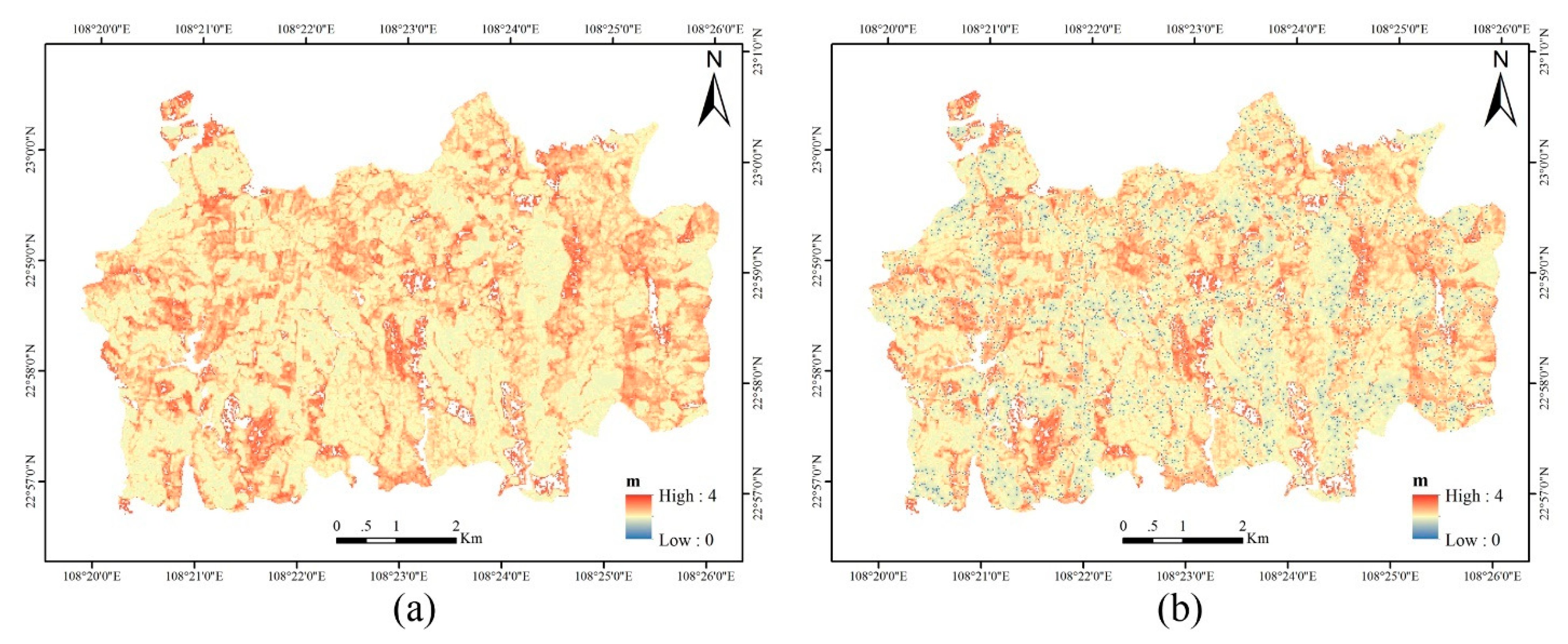
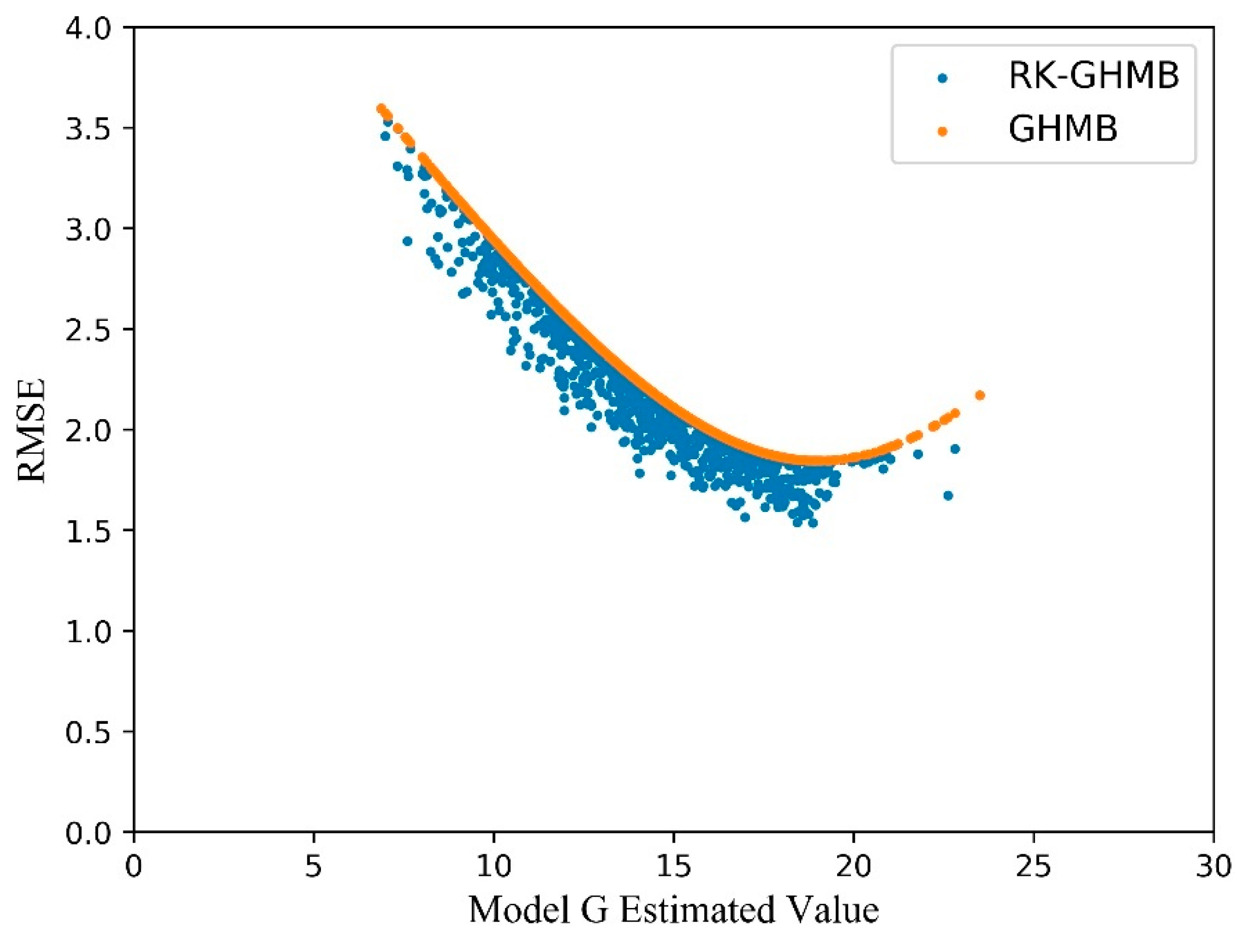
3.3. Forest Canopy Height Estimation Accuracy and Uncertainty Assessment
4. Discussion
5. Conclusions
Author Contributions
Funding
Data Availability Statement
Conflicts of Interest
References
- Le Toan, T.; Quegan, S.; Davidson, M.; Balzter, H.; Paillou, P.; Papathanassiou, K.; Plummer, S.; Rocca, F.; Saatchi, S.; Shugart, H.; et al. The BIOMASS mission: Mapping global forest biomass to better understand the terrestrial carbon cycle. Remote Sens. Environ. 2011, 115, 2850–2860. [Google Scholar] [CrossRef] [Green Version]
- Hese, S.; Lucht, W.; Schmullius, C.; Barnsley, M.; Dubayah, R.; Knorr, D.; Neumann, K.; Riedel, T.; Schröter, K. Global biomass mapping for an improved understanding of the CO2 balance—the Earth observation mission Carbon-3D. Remote Sens. Environ. 2005, 94, 94–104. [Google Scholar] [CrossRef]
- Chen, Q. Modeling aboveground tree woody biomass using national-scale allometric methods and airborne lidar. ISPRS J. Photogramm. Remote Sens. 2015, 106, 95–106. [Google Scholar] [CrossRef]
- Li, D.; Gu, X.; Pang, Y.; Chen, B.; Liu, L. Estimation of Forest Aboveground Biomass and Leaf Area Index Based on Digital Aerial Photograph Data in Northeast China. Forests 2018, 9, 275. [Google Scholar] [CrossRef] [Green Version]
- Houghton, R.A.; Hall, F.; Goetz, S. Importance of biomass in the global carbon cycle. J. Geophys. Res. Earth Surf. 2009, 114, G00E03. [Google Scholar] [CrossRef]
- Andersen, H.-E.; Reutebuch, S.E.; McGaughey, R.J. A rigorous assessment of tree height measurements obtained using airborne lidar and conventional field methods. Can. J. Remote Sens. 2006, 32, 355–366. [Google Scholar] [CrossRef]
- Nelson, R.; Parker, G.; Hom, M. A Portable Airborne Laser System for Forest Inventory. Photogramm. Eng. Remote Sens. 2003, 69, 267–273. [Google Scholar] [CrossRef] [Green Version]
- Stojanova, D.; Panov, P.; Gjorgjioski, V.; Kobler, A.; Džeroski, S. Estimating vegetation height and canopy cover from remotely sensed data with machine learning. Ecol. Inform. 2010, 5, 256–266. [Google Scholar] [CrossRef]
- Ghulam, A.; Porton, I.; Freeman, K. Detecting subcanopy invasive plant species in tropical rainforest by integrating optical and microwave (InSAR/PolInSAR) remote sensing data, and a decision tree algorithm. ISPRS J. Photogramm. Remote Sens. 2014, 88, 174–192. [Google Scholar] [CrossRef]
- Saarela, S.; Wästlund, A.; Holmström, E.; Mensah, A.A.; Holm, S.; Nilsson, M.; Fridman, J.; Ståhl, G. Mapping aboveground biomass and its prediction uncertainty using LiDAR and field data, accounting for tree-level allometric and LiDAR model errors. For. Ecosyst. 2020, 7, 1–17. [Google Scholar] [CrossRef]
- Lagomasino, D.; Fatoyinbo, T.; Lee, S.; Feliciano, E.; Trettin, C.; Simard, M. A Comparison of Mangrove Canopy Height Using Multiple Independent Measurements from Land, Air, and Space. Remote Sens. 2016, 8, 327. [Google Scholar] [CrossRef] [PubMed] [Green Version]
- Babcock, C.; Matney, J.; Finley, A.O.; Weiskittel, A.; Cook, B.D. Multivariate spatial regression models for predicting individual tree structure variables using LiDAR data. IEEE J. Sel. Top. Appl. Earth Obs. Remote Sens. 2012, 6, 6–14. [Google Scholar] [CrossRef]
- Lee, S.; Ni-Meister, W.; Yang, W.; Chen, Q. Physically based vertical vegetation structure retrieval from ICESat data: Vali-dation using LVIS in White Mountain National Forest, New Hampshire, USA. Remote Sens. Environ. 2011, 115, 2776–2785. [Google Scholar] [CrossRef]
- Chen, H.; Cloude, S.R.; Goodenough, D.G.; Hill, D.; Nesdoly, A. Radar Forest Height Estimation in Mountainous Terrain Using Tandem-X Coherence Data. IEEE J. Sel. Top. Appl. Earth Obs. Remote Sens. 2018, 11, 3443–3452. [Google Scholar] [CrossRef]
- Chrysafis, I.; Mallinis, G.; Siachalou, S.; Patias, P. Assessing the relationships between growing stock volume and Sentinel-2 imagery in a Mediterranean forest ecosystem. Remote Sens. Lett. 2017, 8, 508–517. [Google Scholar] [CrossRef]
- Hall, R.; Skakun, R.; Arsenault, E.; Case, B. Modeling forest stand structure attributes using Landsat ETM+ data: Application to mapping of aboveground biomass and stand volume. For. Ecol. Manag. 2006, 225, 378–390. [Google Scholar] [CrossRef]
- Avitabile, V.; Baccini, A.; Friedl, M.A.; Schmullius, C. Capabilities and limitations of Landsat and land cover data for aboveground woody biomass estimation of Uganda. Remote Sens. Environ. 2012, 117, 366–380. [Google Scholar] [CrossRef]
- Chen, G.; Hay, G.J. An airborne lidar sampling strategy to model forest canopy height from Quickbird imagery and GEOBIA. Remote Sens. Environ. 2011, 115, 1532–1542. [Google Scholar] [CrossRef]
- Fayad, I.; Baghdadi, N.; Bailly, J.-S.; Barbier, N.; Gond, V.; Herault, B.; El Hajj, M.; Fabre, F.; Perrin, J. Regional Scale Rain-Forest Height Mapping Using Regression-Kriging of Spaceborne and Airborne LiDAR Data: Application on French Guiana. Remote Sens. 2016, 8, 240. [Google Scholar] [CrossRef] [Green Version]
- Garcia, M.; Saatchi, S.; Ustin, S.; Balzter, H. Modelling forest canopy height by integrating airborne LiDAR samples with satellite Radar and multispectral imagery. Int. J. Appl. Earth Obs. Geoinf. 2018, 66, 159–173. [Google Scholar] [CrossRef]
- Lim, K.; Treitz, P.; Wulder, M.; St-Onge, B.; Flood, M. LiDAR remote sensing of forest structure. Prog. Phys. Geogr. Earth Environ. 2003, 27, 88–106. [Google Scholar] [CrossRef] [Green Version]
- Tian, X.; Su, Z.; Chen, E.; Li, Z.; van der Tol, C.; Guo, J.; He, Q. Estimation of forest above-ground biomass using multi-parameter remote sensing data over a cold and arid area. Int. J. Appl. Earth Obs. Geoinf. 2012, 14, 160–168. [Google Scholar] [CrossRef]
- Ayrey, E.; Hayes, D.J. The Use of Three-Dimensional Convolutional Neural Networks to Interpret LiDAR for Forest Inventory. Remote Sens. 2018, 10, 649. [Google Scholar] [CrossRef] [Green Version]
- Tsui, O.W.; Coops, N.C.; Wulder, M.A.; Marshall, P.L. Integrating airborne LiDAR and space-borne radar via multivariate kriging to estimate above-ground biomass. Remote Sens. Environ. 2013, 139, 340–352. [Google Scholar] [CrossRef]
- Ahmed, O.S.; Franklin, S.E.; Wulder, M.A.; White, J.C. Characterizing stand-level forest canopy cover and height using Landsat time series, samples of airborne LiDAR, and the Random Forest algorithm. ISPRS J. Photogramm. Remote Sens. 2015, 101, 89–101. [Google Scholar] [CrossRef]
- Li, W.; Niu, Z.; Shang, R.; Qin, Y.; Wang, L.; Chen, H. High-resolution mapping of forest canopy height using machine learning by coupling ICESat-2 LiDAR with Sentinel-1, Sentinel-2 and Landsat-8 data. Int. J. Appl. Earth Obs. Geoinf. 2020, 92, 102163. [Google Scholar] [CrossRef]
- Matasci, G.; Hermosilla, T.; Wulder, M.A.; White, J.C.; Coops, N.C.; Hobart, G.W.; Zald, H.S.J. Large-area mapping of Canadian boreal forest cover, height, biomass and other structural attributes using Landsat composites and lidar plots. Remote Sens. Environ. 2018, 209, 90–106. [Google Scholar] [CrossRef]
- Durante, P.; Martín-Alcón, S.; Gil-Tena, A.; Algeet, N.; Tomé, J.L.; Recuero, L.; Palacios-Orueta, A.; Oyonarte, C. Improving Aboveground Forest Biomass Maps: From High-Resolution to National Scale. Remote Sens. 2019, 11, 795. [Google Scholar] [CrossRef] [Green Version]
- Hudak, A.T.; Lefsky, M.A.; Cohen, W.B.; Berterretche, M. Integration of lidar and Landsat ETM+ data for estimating and mapping forest canopy height. Remote Sens. Environ. 2002, 82, 397–416. [Google Scholar] [CrossRef] [Green Version]
- Pouladi, N.; Møller, A.B.; Tabatabai, S.; Greve, M.H. Mapping soil organic matter contents at field level with Cubist, Random Forest and kriging. Geoderma 2019, 342, 85–92. [Google Scholar] [CrossRef]
- Li, S.; Quackenbush, L.J.; Im, J. Airborne Lidar Sampling Strategies to Enhance Forest Aboveground Biomass Estimation from Landsat Imagery. Remote Sens. 2019, 11, 1906. [Google Scholar] [CrossRef] [Green Version]
- Mäkelä, H.; Pekkarinen, A. Estimation of forest stand volumes by Landsat TM imagery and stand-level field-inventory data. For. Ecol. Manag. 2004, 196, 245–255. [Google Scholar] [CrossRef]
- Zhu, X.; Wang, C.; Nie, S.; Pan, F.; Xi, X.; Hu, Z. Mapping forest height using photon-counting LiDAR data and Landsat 8 OLI data: A case study in Virginia and North Carolina, USA. Ecol. Indic. 2020, 114, 106287. [Google Scholar] [CrossRef]
- Potapov, P.; Li, X.; Hernandez-Serna, A.; Tyukavina, A.; Hansen, M.C.; Kommareddy, A.; Pickens, A.; Turubanova, S.; Tang, H.; Silva, C.E.; et al. Mapping global forest canopy height through integration of GEDI and Landsat data. Remote Sens. Environ. 2021, 253, 112165. [Google Scholar] [CrossRef]
- Mohammadi, J.; Joibary, S.S.; Yaghmaee, F.; Mahiny, A.S. Modelling forest stand volume and tree density using Landsat ETM+ data. Int. J. Remote Sens. 2010, 31, 2959–2975. [Google Scholar] [CrossRef]
- Nemmaoui, A.; Aguilar, F.J.; Aguilar, M.A.; Qin, R. DSM and DTM generation from VHR satellite stereo imagery over plastic covered greenhouse areas. Comput. Electron. Agric. 2019, 164, 104903. [Google Scholar] [CrossRef]
- Neigh, C.S.; Masek, J.G.; Bourget, P.; Cook, B.; Huang, C.; Rishmawi, K.; Zhao, F. Deciphering the precision of stereo IKONOS canopy height models for US forests with G-LiHT airborne LiDAR. Remote Sens. 2014, 6, 1762–1782. [Google Scholar] [CrossRef] [Green Version]
- Montesano, P.M.; Neigh, C.; Sun, G.; Duncanson, L.; Hoek, J.V.D.; Ranson, K.J. The use of sun elevation angle for stereogrammetric boreal forest height in open canopies. Remote Sens. Environ. 2017, 196, 76–88. [Google Scholar] [CrossRef] [Green Version]
- Liu, M.; Cao, C.; Chen, W.; Wang, X. Mapping Canopy Heights of Poplar Plantations in Plain Areas Using ZY3-02 Stereo and Multispectral Data. ISPRS Int. J. Geo-Inf. 2019, 8, 106. [Google Scholar] [CrossRef] [Green Version]
- Congalton, R.G. Using spatial autocorrelation analysis to explore the errors in maps generated from remotely sensed data. Photogramm. Eng. Remote Sens. 1988, 54, 587–592. [Google Scholar]
- Steele, B.M.; Winne, J.; Redmond, R.L. Estimation and Mapping of Misclassification Probabilities for Thematic Land Cover Maps. Remote Sens. Environ. 1998, 66, 192–202. [Google Scholar] [CrossRef]
- Wang, G.; Oyana, T.; Zhang, M.; Adu-Prah, S.; Zeng, S.; Lin, H.; Se, J. Mapping and spatial uncertainty analysis of forest vegetation carbon by combining national forest inventory data and satellite images. For. Ecol. Manag. 2009, 258, 1275–1283. [Google Scholar] [CrossRef]
- Lu, D.; Chen, Q.; Wang, G.; Moran, E.F.; Batistella, M.; Zhang, M.; Laurin, G.V.; Saah, D. Aboveground Forest Biomass Estimation with Landsat and LiDAR Data and Uncertainty Analysis of the Estimates. Int. J. For. Res. 2012, 2012, 436537. [Google Scholar] [CrossRef]
- Mahoney, C.; Hall, R.J.; Hopkinson, C.; Filiatrault, M.; Beaudoin, A.; Chen, Q. A Forest Attribute Mapping Framework: A Pilot Study in a Northern Boreal Forest, Northwest Territories, Canada. Remote Sens. 2018, 10, 1338. [Google Scholar] [CrossRef] [Green Version]
- Varvia, P.; Lähivaara, T.; Maltamo, M.; Packalen, P.; Tokola, T.; Seppänen, A. Uncertainty quantification in ALS-based species-specific growing stock volume estimation. IEEE Trans. Geosci. Remote Sens. 2016, 55, 1671–1681. [Google Scholar] [CrossRef]
- Urbazaev, M.; Thiel, C.; Cremer, F.; Dubayah, R.; Migliavacca, M.; Reichstein, M.; Schmullius, C. Estimation of forest above-ground biomass and uncertainties by integration of field measurements, airborne LiDAR, and SAR and optical satellite data in Mexico. Carbon Balance Manag. 2018, 13, 1–20. [Google Scholar] [CrossRef] [PubMed] [Green Version]
- Fang, S.; Gertner, G.Z.; Anderson, A.A. Estimation of sensitivity coefficients of nonlinear model input parameters which have a multinormal distribution. Comput. Phys. Commun. 2004, 157, 9–16. [Google Scholar] [CrossRef]
- Gonzalez, P.; Asner, G.P.; Battles, J.J.; Lefsky, M.A.; Waring, K.M.; Palace, M. Forest carbon densities and uncertainties from Lidar, QuickBird, and field measurements in California. Remote Sens. Environ. 2010, 114, 1561–1575. [Google Scholar] [CrossRef]
- Lang, N.; Kalischek, N.; Armston, J.; Schindler, K.; Dubayah, R.; Wegner, J.D. Global canopy height regression and uncertainty estimation from GEDI LIDAR waveforms with deep ensembles. Remote Sens. Environ. 2022, 268, 112760. [Google Scholar] [CrossRef]
- Saarela, S.; Holm, S.; Grafström, A.; Schnell, S.; Næsset, E.; Gregoire, T.G.; Nelson, R.F.; Ståhl, G. Hierarchical model-based inference for forest inventory utilizing three sources of information. Ann. For. Sci. 2016, 73, 895–910. [Google Scholar] [CrossRef] [Green Version]
- Saarela, S.; Holm, S.; Healey, S.P.; Andersen, H.-E.; Petersson, H.; Prentius, W.; Patterson, P.L.; Næsset, E.; Gregoire, T.G.; Ståhl, G. Generalized Hierarchical Model-Based Estimation for Aboveground Biomass Assessment Using GEDI and Landsat Data. Remote Sens. 2018, 10, 1832. [Google Scholar] [CrossRef] [Green Version]
- Pang, Y.; Li, Z.; Ju, H.; Lu, H.; Jia, W.; Si, L.; Guo, Y.; Liu, Q.; Li, S.; Liu, L.; et al. LiCHy: The CAF’s LiDAR, CCD and Hyperspectral Integrated Airborne Observation System. Remote Sens. 2016, 8, 398. [Google Scholar] [CrossRef] [Green Version]
- McRoberts, R.E. A model-based approach to estimating forest area. Remote Sens. Environ. 2006, 103, 56–66. [Google Scholar] [CrossRef]
- Ribeiro, P.J., Jr.; Diggle, P.J.; Christensen, O.; Schlather, M.; Bivand, R.; Ripley, B. GeoR: Analysis of Geostatistical Data. Available online: http://www.leg.ufpr.br/geoR (accessed on 10 February 2020).
- Hengl, T.; Heuvelink, G.B.; Stein, A. A generic framework for spatial prediction of soil variables based on regression-kriging. Geoderma 2004, 120, 75–93. [Google Scholar] [CrossRef] [Green Version]
- Lu, D. Aboveground biomass estimation using Landsat TM data in the Brazilian Amazon. Int. J. Remote Sens. 2005, 26, 2509–2525. [Google Scholar] [CrossRef]
- Odeh, I.O.; McBratney, A.B.; Chittleborough, D.J. Further results on prediction of soil properties from terrain attributes: Het-erotopic cokriging and regression-kriging. Geoderma 1995, 67, 215–226. [Google Scholar] [CrossRef]
- Cressie, N.A. Statistics for Spatial Data, 3rd ed.; John Wiley & Sons, Inc.: New York, NY, USA, 1993; pp. 151–155. [Google Scholar]
- Pinheiro, J.; Bates, D.; DebRoy, S.; Sarkar, D. nlme: Linear Nonlinear Mixed Effects Models. Available online: https://cran.r-project.org/package=nlme (accessed on 13 January 2022).
- Lado, L.R.; Polya, D.; Winkel, L.; Berg, M.; Hegan, A. Modelling arsenic hazard in Cambodia: A geostatistical approach using ancillary data. Appl. Geochem. 2008, 23, 3010–3018. [Google Scholar] [CrossRef]
- Gu, C.; Clevers, J.G.; Liu, X.; Tian, X.; Li, Z.; Li, Z. Predicting forest height using the GOST, Landsat 7 ETM+, and airborne LiDAR for sloping terrains in the Greater Khingan Mountains of China. ISPRS J. Photogramm. Remote Sens. 2018, 137, 97–111. [Google Scholar] [CrossRef]
- Wulder, M.A.; White, J.C.; Nelson, R.F.; Næsset, E.; Ørka, H.O.; Coops, N.C.; Hilker, T.; Bater, C.W.; Gobakken, T. Lidar Sampling for Large-Area Forest Characterization: A Review. Remote Sens. Environ. 2012, 121, 196–209. [Google Scholar] [CrossRef] [Green Version]
- Viana, H.; Aranha, J.; Lopes, D.; Cohen, W.B. Estimation of crown biomass of Pinus pinaster stands and shrubland above-ground biomass using forest inventory data, remotely sensed imagery and spatial prediction models. Ecol. Model. 2012, 226, 22–35. [Google Scholar] [CrossRef]
- Li, W.; Niu, Z.; Liang, X.; Li, Z.; Huang, N.; Gao, S.; Wang, C.; Muhammad, S. Geostatistical modeling using LiDAR-derived prior knowledge with SPOT-6 data to estimate temperate forest canopy cover and above-ground biomass via stratified random sampling. Int. J. Appl. Earth Obs. Geoinf. 2015, 41, 88–98. [Google Scholar] [CrossRef]
- Silveira, E.M.; Santo, F.D.E.; Wulder, M.A.; Júnior, F.W.A.; Carvalho, M.C.; Mello, C.R.; Mello, J.M.; Shimabukuro, Y.E.; Terra, M.C.N.S.; Carvalho, L.M.T.; et al. Pre-stratified modelling plus residuals kriging reduces the uncertainty of aboveground biomass estimation and spatial distribution in heterogeneous savannas and forest environments. For. Ecol. Manag. 2019, 445, 96–109. [Google Scholar] [CrossRef]
- Chen, L.; Ren, C.; Zhang, B.; Wang, Z. Multi-Sensor Prediction of Stand Volume by a Hybrid Model of Support Vector Machine for Regression Kriging. Forests 2020, 11, 296. [Google Scholar] [CrossRef] [Green Version]
- Mauro, F.; Monleon, V.; Temesgen, H.; Ruiz, L. Analysis of spatial correlation in predictive models of forest variables that use LiDAR auxiliary information. Can. J. For. Res. 2017, 47, 788–799. [Google Scholar] [CrossRef] [Green Version]
- Fan, W.B.; Zhao, C.J.; Lin, Z.; Chen, H. Growth Characteristics of Eucalyptus Plantation and Their Responses to Climate En-vironment in Western Hainan Island. For. Resour. Manag. 2013, 4, 77–82. [Google Scholar]


| Parameters | Value | Parameters | Value |
|---|---|---|---|
| Platform | Tecnam P2006T | Flying height (m) | 1000 |
| Laser beam divergence (m·rad) | 0.5 | Speed (Km·h−1) | 180 |
| Laser wavelength (nm) | 1550 | Vertical accuracy (cm) | 15 |
| Scan angle (°) | ±30 | Average point density (points·m−2) | 8.51 |
| Laser pulse repetition rate (kHz) | 400 | Pulse length (ns) | 3 |
| Model Name | Model Forms | R2 | RMSE | |
|---|---|---|---|---|
| F | (17) | 0.75 | 1.81 | |
| G | (18) | 0.64 | 2.38 | |
| (19) | 0.81 | 1.01 |
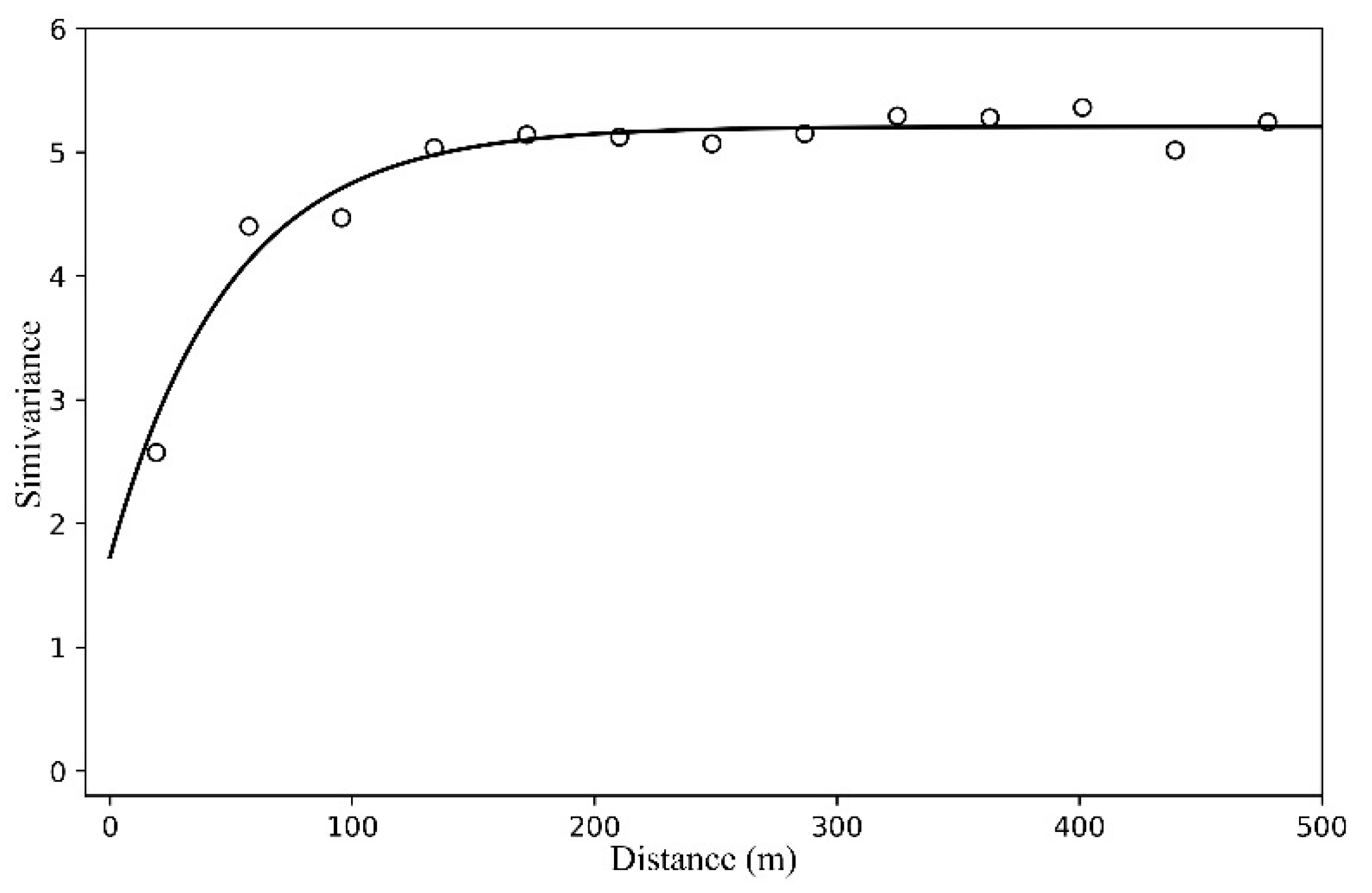
| Residuals Source | Model | Nugget (C0) | Partial Sill (C1) | Range (m) | Ratio (%) |
|---|---|---|---|---|---|
| Model G | exponential | 1.73 | 3.48 | 147.27 | 33.2 |
| Plot-Based Reference | LiDAR-Based Reference | |||
|---|---|---|---|---|
| Models | ||||
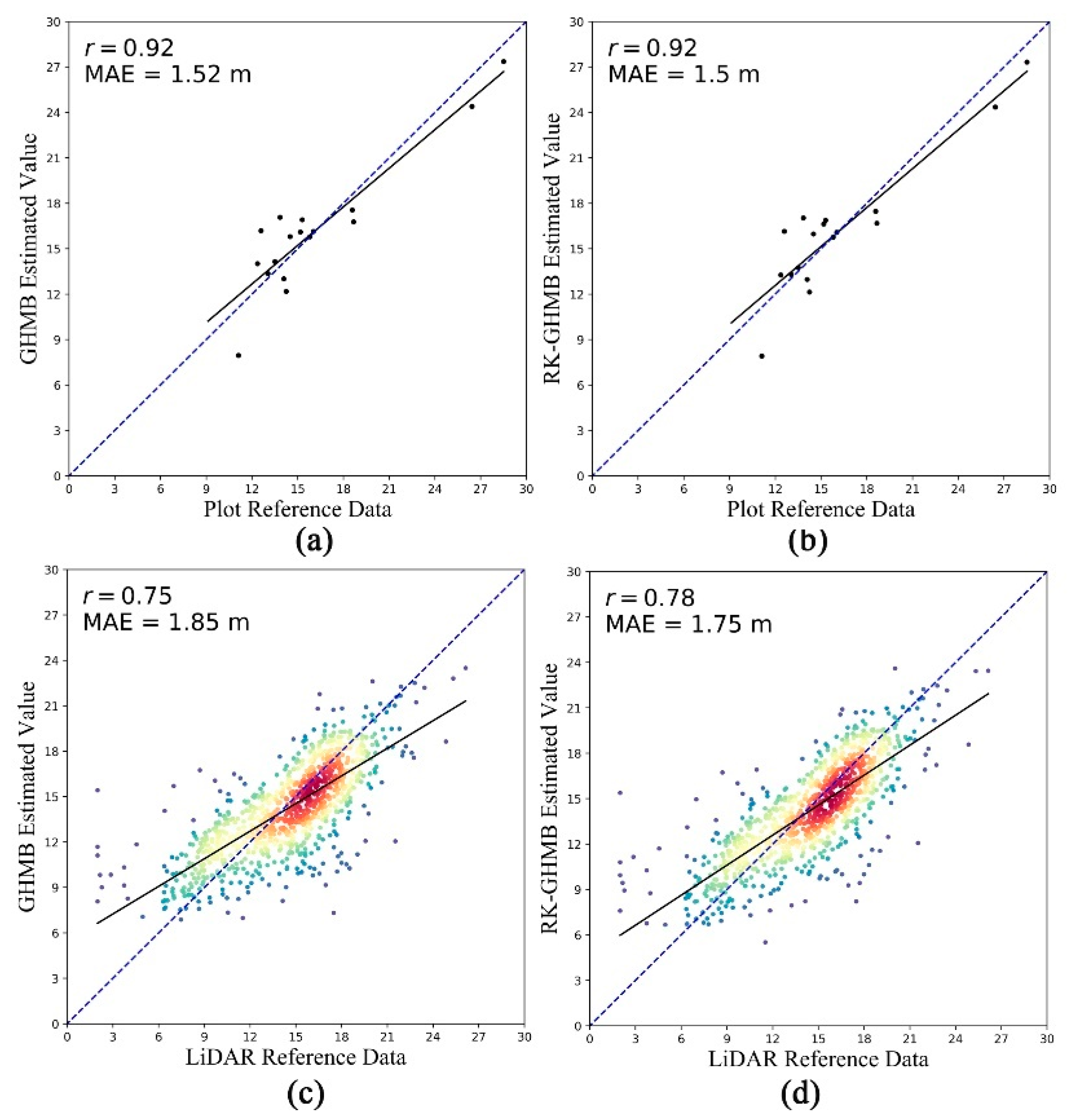
| GHMB | 0.92 | 1.52 | 0.75 | 1.85 |
| RK-GHMB | 0.92 | 1.50 | 0.78 | 1.75 |
Publisher’s Note: MDPI stays neutral with regard to jurisdictional claims in published maps and institutional affiliations. |
© 2022 by the authors. Licensee MDPI, Basel, Switzerland. This article is an open access article distributed under the terms and conditions of the Creative Commons Attribution (CC BY) license (https://creativecommons.org/licenses/by/4.0/).
Share and Cite
Zhao, J.; Zhao, L.; Chen, E.; Li, Z.; Xu, K.; Ding, X. An Improved Generalized Hierarchical Estimation Framework with Geostatistics for Mapping Forest Parameters and Its Uncertainty: A Case Study of Forest Canopy Height. Remote Sens. 2022, 14, 568. https://doi.org/10.3390/rs14030568
Zhao J, Zhao L, Chen E, Li Z, Xu K, Ding X. An Improved Generalized Hierarchical Estimation Framework with Geostatistics for Mapping Forest Parameters and Its Uncertainty: A Case Study of Forest Canopy Height. Remote Sensing. 2022; 14(3):568. https://doi.org/10.3390/rs14030568
Chicago/Turabian StyleZhao, Junpeng, Lei Zhao, Erxue Chen, Zengyuan Li, Kunpeng Xu, and Xiangyuan Ding. 2022. "An Improved Generalized Hierarchical Estimation Framework with Geostatistics for Mapping Forest Parameters and Its Uncertainty: A Case Study of Forest Canopy Height" Remote Sensing 14, no. 3: 568. https://doi.org/10.3390/rs14030568