Article

The Joint Assimilation of Remotely Sensed Leaf Area Index and Surface Soil Moisture into a Land Surface Model

1
Department of Civil, Environmental, and Infrastructure Engineering, George Mason University, Fairfax, VA 22030, USA
2
Department of Civil and Environmental Engineering, University of Connecticut, Storrs, CT 06269, USA
3
Department of Geography and Geoinformation Science, George Mason University, Fairfax, VA 22030, USA
4
Department of Mathematics, George Mason University, Fairfax, VA 22030, USA
5
SAIC at NASA Goddard Space Flight Center, Greenbelt, MD 20771, USA
*
Author to whom correspondence should be addressed.
Remote Sens. 2022, 14(3), 437; https://doi.org/10.3390/rs14030437
Submission received: 8 December 2021 / Revised: 11 January 2022 / Accepted: 14 January 2022 / Published: 18 January 2022

Abstract

:
This work tests the hypothesis that jointly assimilating satellite observations of leaf area index and surface soil moisture into a land surface model improves the estimation of land vegetation and water variables. An Ensemble Kalman Filter is used to test this hypothesis across the Contiguous United States from April 2015 to December 2018. The performance of the proposed methodology is assessed for several modeled vegetation and water variables (evapotranspiration, net ecosystem exchange, and soil moisture) in terms of random errors and anomaly correlation coefficients against a set of independent validation datasets (i.e., Global Land Evaporation Amsterdam Model, FLUXCOM, and International Soil Moisture Network). The results show that the assimilation of the leaf area index mostly improves the estimation of evapotranspiration and net ecosystem exchange, whereas the assimilation of surface soil moisture alone improves surface soil moisture content, especially in the western US, in terms of both root mean squared error and anomaly correlation coefficient. The joint assimilation of vegetation and soil moisture information combines the results of individual vegetation and soil moisture assimilations and reduces errors (and increases correlations with the reference datasets) in evapotranspiration, net ecosystem exchange, and surface soil moisture simulated by the land surface model. However, because soil moisture satellite observations only provide information on the water content in the top 5 cm of the soil column, the impact of the proposed data assimilation technique on root zone soil moisture is limited. This work moves one step forward in the direction of improving our estimation and understanding of land surface interactions using a multivariate data assimilation approach, which can be particularly useful in regions of the world where ground observations are sparse or missing altogether.

Graphical Abstract

1. Introduction

Vegetation and soil moisture both play very important roles in land surface modeling by supporting critical functions in the global and regional water and energy cycles. Vegetation impacts soil characteristics, e.g., its water content, chemistry, and texture, that have feedback on vegetation characteristics, including productivity and structure [1]. Soil moisture represents the land storage for water and energy, effectively controlling the balance between sensible and latent heat flux at the land–atmosphere interface. Soil moisture content impacts atmospheric processes, such as cloud coverage and rainfall, thus affecting hydrological processes such as runoff and plant transpiration [2,3].
To represent vegetation structural and functional variables, dynamic vegetation models (DVMs) have been designed [4]. In the past, DVMs and land surface models (LSMs) have been combined to improve the estimation of water, carbon, and energy variables [5,6]. As an example, the Noah Multi-Parameterization LSM (hereinafter Noah-MP), which was developed by Niu et al. [7], combines an LSM with a DVM, using a module that allocates carbon to various parts of vegetation and soil carbon pools. However, land surface models are affected by several uncertainties because of different reasons, such as inaccurate initialization, mis-specified forcing and parameters, or inadequate model physics [8].
As an alternative to model simulations, satellite observations also offer the estimations of several land surface variables over the global domain. For vegetation, satellites produce maps of the leaf area index (LAI), defined as the single-sided leaf surface area estimated over the unit ground area, and normalized difference vegetation index (NDVI), estimated by spectral reflectance measurements received in the red and near-infrared regions [9]. For example, the Moderate Resolution Imaging Spectroradiometer (MODIS), which has been receiving data in 36 spectral bands since 2000 [10], and the Advanced Very High-Resolution Radiometer (AVHRR; [11]) produce global maps of vegetation indices. Satellite observations also provide soil moisture information. For instance, the Soil Moisture Active Passive (SMAP; [12]) mission launched in 2015 provides direct sensing of soil moisture in the top 5 cm of the soil column.
Satellite-based observations are affected by gaps in both spatial and temporal coverages (often because of cloud coverage or instrument malfunctioning). To address the gaps in satellite observations and reduce uncertainties in both models and observations, data assimilation (DA) can be adopted to optimally combine the information from observations and model estimates [13]. Land Data Assimilation Systems (LDASs) have been used in the past successfully for merging satellite observations into LSMs [3,13,14]. DA has the potential to improve model estimates of land surface variables, which is useful for different purposes, including the monitoring and forecasting of extreme hydrological events, crop water management, and ecological studies. DA can be particularly effective in data-poor regions, where ground observations are sparse or not available at all.
Soil moisture has been assimilated in land surface models to generate a superior soil moisture product in numerous experiments, which used field measurements and satellite retrievals [3]. For large-scale soil moisture DA, the Ensemble Kalman Filter (EnKF) has become a method of choice [15,16]. Reichle et al. [17] performed a comparison between the Extended Kalman Filter and the EnKF for soil moisture estimation in a twin experiment over the southeastern United States, and both methods provided satisfactory estimates of soil moisture. In the last decade, real satellite soil moisture observations have been used in several experiments for DA within different land surface models [18,19,20,21,22,23].
More recent studies have applied DA techniques to vegetation observations and vegetation dynamic models. For instance, Kumar et al. [24] performed an experiment to assess the impact of satellite-based LAI DA by applying an EnKF technique to the Noah-MP LSM over the Continental U.S. (CONUS). The results showed that LAI DA improves the estimation of key water budget terms (i.e., soil moisture, evapotranspiration (ET), terrestrial water storage, and streamflow) and carbon fluxes (i.e., gross primary production and net ecosystem exchange) when validated with ground-based reference datasets, but the improvement in surface soil moisture was still limited. In another study, Ling et al. [25] assimilated Global Land Surface Satellite (GLASS) LAI data using an Ensemble Adjustment Kalman Filter technique over the global domain. The results demonstrated that the DA reduced the bias in LAI (from 5 m2/m2 to ±1 m2/m2). Two past studies proposed synthetic experiments to assimilate LAI alone within Noah-MP using an EnKF [26] and direct insertion (DI) [9]. The results showed an improvement in a subset of water and vegetation variables and a reduction in the impact of large biases in the model input precipitation. However, the improvement in soil moisture was still limited.
Past work that jointly assimilated vegetation and water variables has shown some promise. As an example, Xie et al. [27] assimilated LAI and surface soil moisture observations within the CERES-Wheat model for winter wheat yield estimation, using a particle filter algorithm across the Guan Zhong Plain, China. Another study jointly assimilated LAI and soil moisture from Sentinel-1 and Sentinel-2 data into a crop model for winter wheat yield estimation in Heng Shui city, China. Although promising, these studies focused on regions of limited spatial extension [28]. A study by Bonan et al. [8] investigated the joint assimilation of surface soil moisture and LAI within the Land Data Assimilation System LDAS-Monde over the Euro-Mediterranean Region. They adopted a deterministic ensemble square root filter. This joint assimilation was shown to moderately improve ET and highly improve river discharges. LDAS-Monde was developed for performing data assimilation using the ISBA (Interaction Sol-Biosphère-Atmosphère) land surface model, initially developed for France and then extended to the global domain [29]. ISBA interfaces with an atmospheric and a hydrological model but simulates above-ground plant biomass and LAI with a simplistic plant growth model (ISBA-A-gs) [30]. In another recent work, Albergel et al. [31] performed a joint assimilation of satellite-derived LAI and soil water index into the ISBA model to monitor the impact of extreme events (heat waves and droughts), using the Simplified Extended Kalman Filter.
This work stems from the studies discussed above and further investigates the potential of jointly assimilating satellite LAI and soil moisture products. Specifically, for the first time, it jointly assimilates GLASS LAI and SMAP soil moisture within the Noah-MP model over the CONUS domain. Noah-MP uses a more sophisticated dynamic vegetation model scheme compared to other similar models used in the literature (e.g., ISBA) [31]. As past work showed that LAI assimilation alone could not improve the estimation of soil moisture (specifically surface soil moisture), the main goal of this work is to improve our estimation and understanding of soil moisture storages in addition to analyzing the impact on vegetation variables.

2. Materials and Methods

The Noah-MP LSM is used to test the hypothesis that, by combining satellite LAI and soil moisture observations within a land surface model, the estimation of vegetation and water variables can be improved. The experiment was run from 1 April 2015 to 31 December 2018 over the CONUS domain (Figure 1).

2.1. The Noah-MP Land Surface Model

The Noah-MP model is based on a semi-tile sub grid scheme, where energy and carbon fluxes are computed separately over two tiles: the fractional vegetated area and the fractional bare ground area [7,32]. There are multiple options for surface water infiltration, runoff, groundwater transfer and storage, dynamic vegetation, canopy resistance, and frozen soil physics in the Noah-MP model [33]. For the dynamic vegetation model of Noah-MP, the Ball–Berry scheme [33] is implemented, which allocates carbon to vegetation leaves, stems, wood, and roots and to soil carbon fast and slow pools.
The Modern-Era Retrospective analysis for Research and Applications, version 2 (MERRA-2 [18]) dataset is used to force the Noah-MP model. Specifically, atmospheric temperature, radiation, water vapor, precipitation, wind speed, topography, altitude forcing variables from the MERRA-2 dataset are used as input to the Noah-MP model in this study (Table 1).
The general model parameters in Noah-MP 3.6 are the slope type, vegetation effect on soil heat, soil evaporation, soil heat capacity, surface runoff parameterization, depth of lower boundary, and soil temperature. This model also uses saturation soil moisture content, soil conductivity, soil diffusivity, wilting point of soil moisture, rooting depth, minimum stomatal resistance, minimum and maximum background emissivity, minimum and maximum background albedo, minimum and maximum background roughness, optimum transpiration in air temperature, canopy water capacity [7,34].
The NASA Land Information System (LIS [35]) framework is used in this work to run the Noah-MP model and implement the DA scheme. LIS provides a framework for ensemble land surface modeling on grid points across the global land and can be run at high resolutions. Noah-MP was not recalibrated ad hoc for this experiment.

2.2. Satellite-Based Observations

In this work, the satellite-based LAI from the GLASS product is merged within the land surface model. The GLASS LAI product is generated using a general regression neural network approach, which allows a spatially and temporally consistent long-term record of vegetation conditions [36]. Two sources, MODIS and AVHRR, provide input to this dataset. MODIS data are available for 2000–2018 and the AVHRR data are available for 1981–2018. The MODIS-based GLASS LAI V50 product is used in this work, which was preferred over the original MODIS LAI product because of the cloud obstruction gaps present in the latter [37].
The SMAP mission provides direct sensing of soil moisture. The SMAP satellite was launched on 2015 by National Aeronautics and Space Administration (NASA). It provides soil moisture data in the top 5 cm of the soil column during 2015–present. The SMAP satellite is in a 6 AM/6 PM ascending and descending orbit, but retrieving soil moisture from the morning overpasses is the primary objective of SMAP [38]. SMAP Level 1 delivers products from its instrument measurements and Level 2 delivers SMAP’s Swath based geographical retrievals [38]. The SMAP Level 3 (SPL3SMP) product, which is used in this work, is a composite based on daily passive radiometer estimates of global land SM at the top 5 cm of the soil that is resampled to a global, cylindrical ~36 km Equal-Area Scalable Earth Grid [39]. A summary of the main characteristics of GLASS LAI and the SMAP soil moisture product used in this study is shown in Table 1.

2.3. Validation Dataset

Different ground and remotely sensed observations are used as independent datasets to validate the proposed system. These observations are obtained from three main sources: the Global Land Evaporation Amsterdam Model (GLEAM), the FLUXCOM datasets, and the International Soil Moisture Network (ISMN). Details regarding the resolution and the time series availability of these datasets are presented in Table 1.
GLEAM is a set of algorithms that separately estimate the different components of land evaporation (or ET): transpiration, bare-soil evaporation, interception loss, open-water evaporation, and sublimation [40,41]. The GLEAM evapotranspiration data are derived from Priestley and Taylor’s evaporation definition and based on remote sensing observations of surface net radiation and near-surface temperature. The GLEAM dataset is freely available at monthly and yearly scales and has been continuously revised and updated since its development in 2011, with a new version introduced in 2017 [40]. This version is used in this study for validating the proposed DA system. GLEAM data have shown good agreement with a number of ground-based observations (e.g., FLUXNET, AU-ASM) [42,43] and have been widely used in the literature [8,24,31,42,43]. The most recent version, GLEAM v3.3b, was chosen in this study to validate the proposed DA system.
The FLUXCOM dataset is derived from a combination of FLUXNET site observations, satellite remote sensing, and meteorological data. A machine learning technique is adopted for estimating the FLUXCOM Gross Primary Production (GPP) and the Net Ecosystem Exchange (NEE). Previous research shows that estimates of seasonal NEE from FLUXCOM provide useful information and are widely used as the validation dataset [44,45,46,47,48]. FLUXCOM is chosen here for its wide availability throughout the CONUS domain during the time span of the experiment and its quality [49,50]. In this work, FLUXCOM NEE has been used to validate the model NEE output.
ISMN is an international global in situ soil moisture database. This network is a joint effort of the Global Energy and Water Exchanges Project (GEWEX), the Committee on Earth Observation Satellites (CEOS), the Global Climate Observing System-Terrestrial Observation Panel for Climate (GCOS-TOPC), the Group of Earth Observation (GEO), and the Global Terrestrial Network on Hydrology (GTN-H) [51]. ISMN soil moisture observations are automatically checked for outliers and transformed into volumetric units. ISMN soil moisture observations are automatically checked for outliers and transformed into volumetric unit. These data have been widely used as a reference in the past, as proven by the existing literature e.g., [8,24,31,52,53]. ISMN provides soil water content at different depths; in this work, observations at 0.1 m depth are considered as surface soil moisture (SSM) and the 1 m depth is considered representative of root zone soil moisture (RZSM).

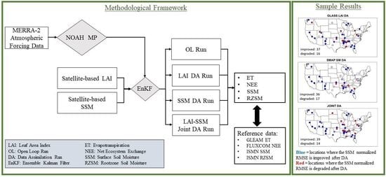
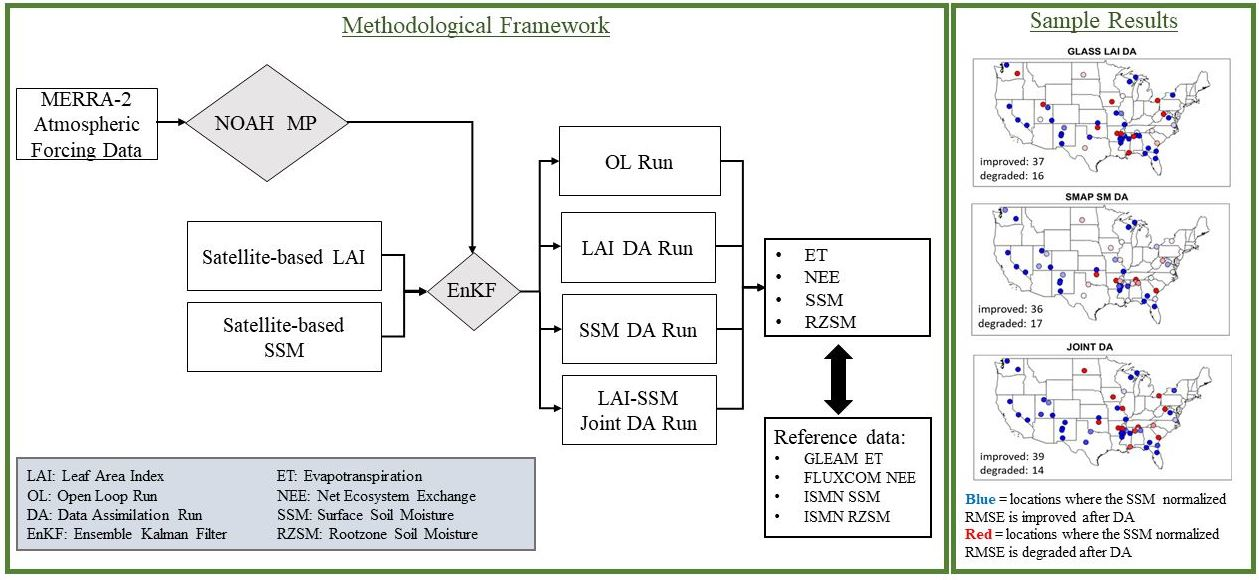
2.4. The Data Assimilation System

EnKF, an approximated version of the traditional Kalman filter based on Monte Carlo simulations, was used as the DA technique in this experiment. In the EnKF, the state probability distribution is represented by a sample (or ensemble), propagated forward in time and updated when a new observation becomes available [14,17,54]. The EnKF technique has flexibility in treating errors in model equations and parameters and is particularly suitable for nonlinear problems, such as soil dynamics [20,55]. Twenty ensemble members are generated by perturbing the atmospheric forcing following the same methodology presented in [24,26]. The precipitation and shortwave radiation are perturbed via multiplicative error models, whereas an additive perturbation is used for longwave radiation.
GLASS LAI observations are perturbed via an additive model with a standard deviation of 0.1. Following Kumar et al. [24], leaf mass is also updated with LAI in this experiment. The observation perturbations for the SMAP product follow an additive model, with zero mean and a standard deviation of 0.04 m3/m3. Additionally, a cumulative distribution function (CDF) matching was applied prior to the SMAP DA as a scaling strategy to remove any existing bias between the satellite observations and model estimation, following the approach developed by Reichle et al., 2004 [56].
The model was spun up for 15 years (2001–1 April 2015) to set the system to an initial equilibrium. A total of four experiments were run: (i) an open-loop (OL) simulation, in which no assimilation is performed; (ii) a DA run that only merges GLASS LAI; (iii) a DA run that only merges SMAP soil moisture; and (iv) a DA run that jointly merges GLASS LAI and SMAP soil moisture.

2.5. System Evaluation

To evaluate the proposed methodology, ET, NEE, and soil moisture from the OL run and the three DA simulations are compared to a set of reference data, described in Section 2.4. Specifically, measurements from the FLUXCOM and GLEAM datasets are used to validate modeled ET and NEE, respectively. The ISMN soil moisture dataset is adopted in this work for validating model simulations of SSM and RZSM. To ease the validation procedure, the validation data were converted to the resolution of the model outputs (0.5° × 0.625°) by simply averaging all points falling within the model grid cell. All three DA experiments were evaluated in terms of ET, NEE, SSM, and RZSM.
Two metrics were used to evaluate the proposed methodology: the Normalized and Centered Root Mean Square Error (NCRMSE) and the Anomaly Correlation Coefficient (ACC). Biases were not evaluated in this study for various reasons. First off, a major assumption of the EnKF is the unbiasedness between model states and observations [57]. Secondly, satellite products, model estimates, and ground observations are different in nature (e.g., point vs. pixel estimate, soil depth for soil moisture) and should therefore be considered as indicators of a specific water/vegetation variable, rather than its perfect approximation.
The NCRMSE is adopted as a measure of the random error [9,26,58,59]:
NCRMSE =   ( ( ( x ^   ( x ^ ) N ) ( X obs   ( X obs ) N ) )   2 ) N   ( X obs ) N
where x ^ represents the model output (DA or OL), Xobs is the related observed variable, and N represents the number of days.
To determine if the DA improves or degrades the estimation of a specific variable with respect to the original (OL) model run, the Normalized Information Contribution (NIC; [24,26]) for NCRMSE is computed as follows:
NIC NCRMSE = NCRMSE DA NCRMSE OL 0 NCRMSE OL
where NICNCRMSE is the NIC for NCRMSE, NCRMSEDA is the NCRMSE of the DA output, and NCRMSEOL is the NCRMSE for the OL output. A NIC value of 1 corresponds to the DA maximum possible improvement over the OL; a value of zero of NIC means that DA and OL have the same performance; and a negative NIC indicates a model degradation through DA [26]. NIC is a unitless metric.
The daily ACC is calculated for the OL and DA model outputs with respect to the reference observations. Anomalies are defined here as the differences between daily values and the yearly climatological average. Each of the anomaly time series is computed relative to the mean of its respective model run. The ACC metric, regardless of potential mean biases or differences in dynamic range, captures the correspondence in phase between model estimates and the reference data [60]. ACC is defined as follows:
ACC =   ( ( x ^   ( x ^ ) N ) ( X obs   ( X obs ) N ) )   ( x ^   ( x ^ ) N ) 2   ( X obs   ( X obs ) N ) 2
where x ^ represents the model output (DA or OL), Xobs is the corresponding observed variable from ground or satellite observations, and N represents the number of days.
For investigating the improvement in ACC due to DA, the difference between ACC in the DA run and OL is as follows:
diff ACC =   ACC DA ACC OL
If diffACC is positive (negative), the DA output has higher (lower) correlation with the observed data than the OL output. ACC is unitless.

3. Results

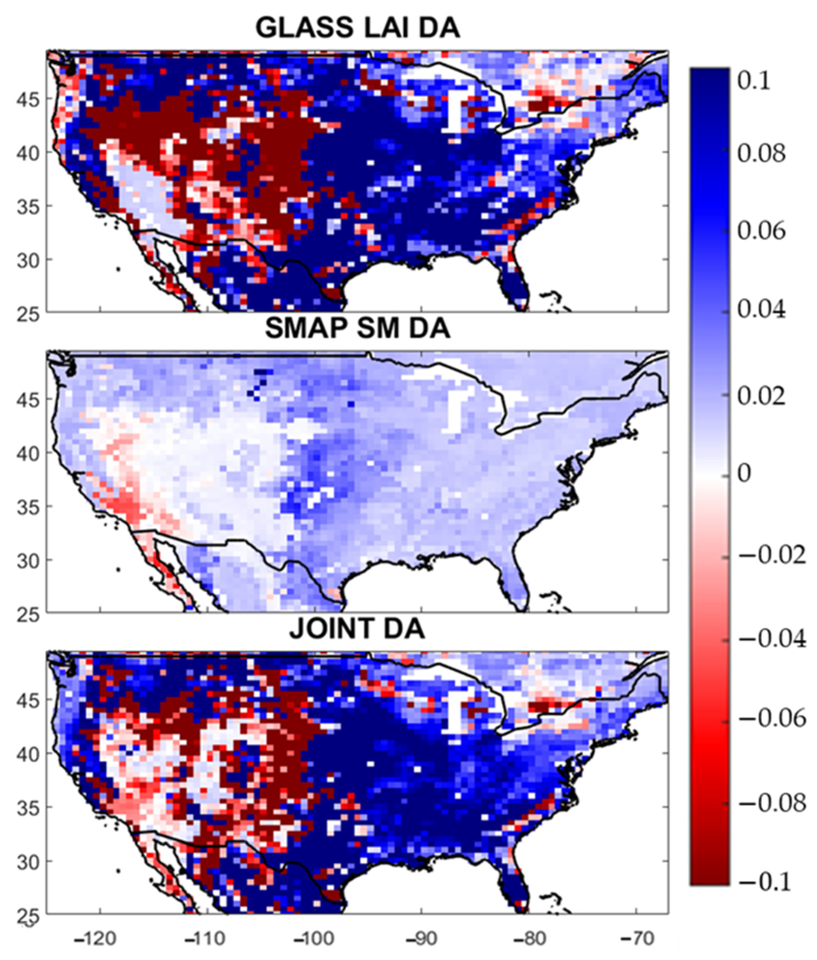
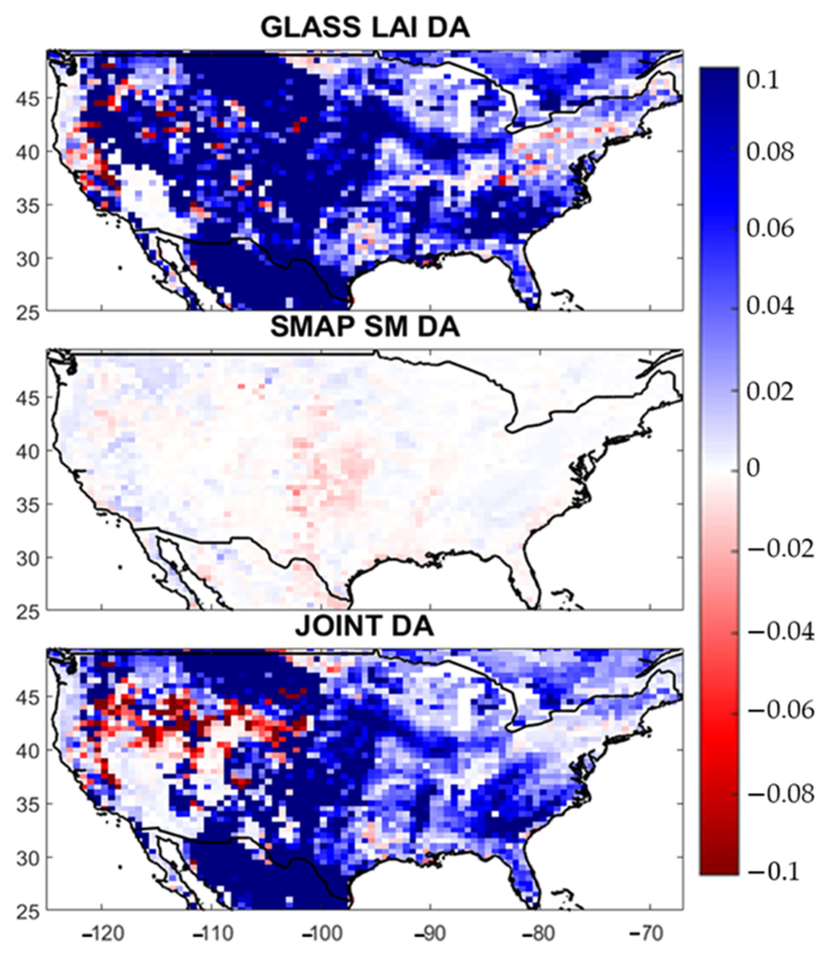
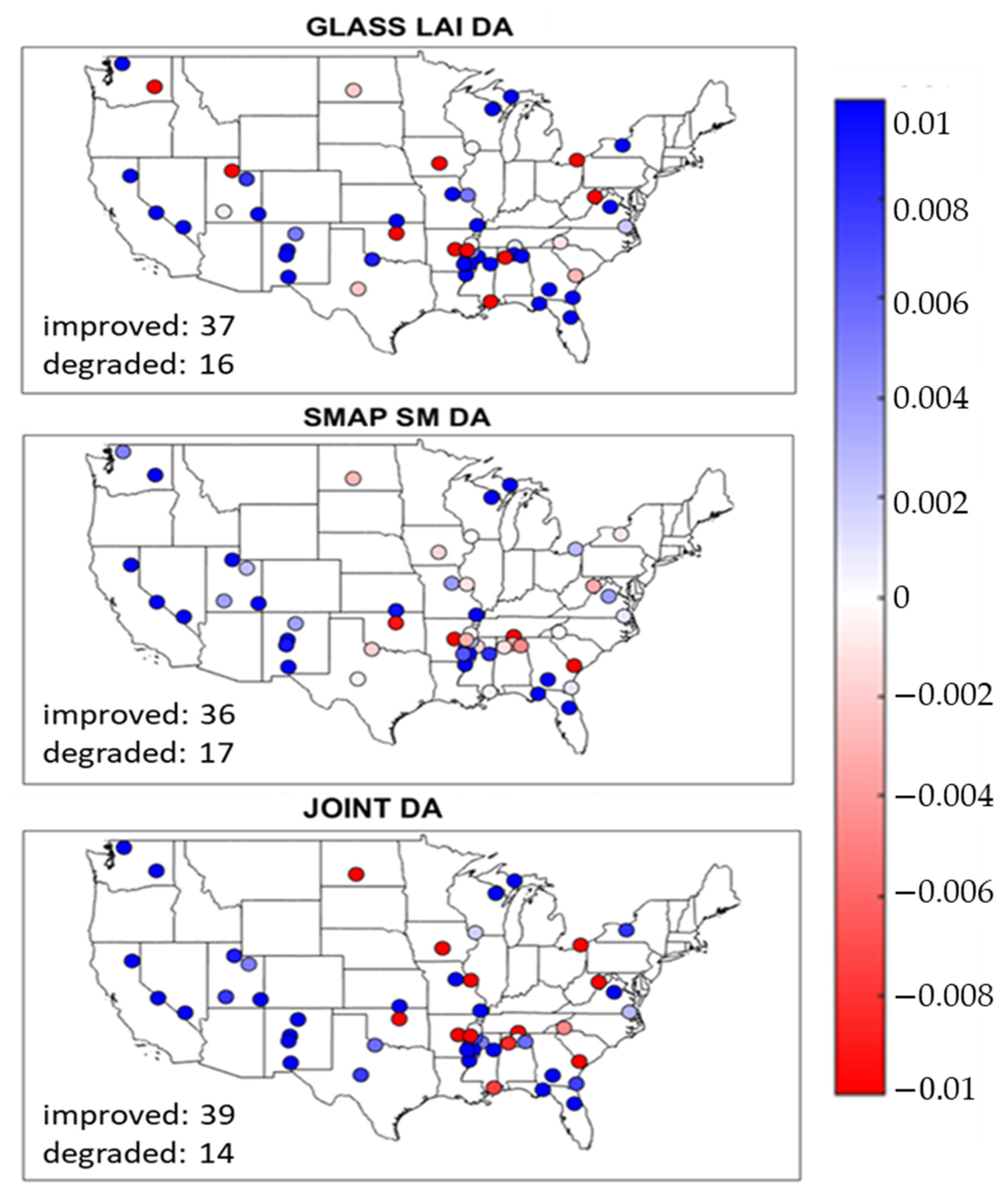
3.1. Impact of Data Assimilation

In order to assess how the proposed DA techniques impact the updated variables, Figure 2 shows the percentage changes between DA and OL for the set of variables of interest in this study: LAI, ET, NEE, SSM, and RZSM. First, all three DA approaches have an impact on the model estimation of these variables. Specifically, the GLASS LAI DA and the joint (GLASS LAI and SMAP soil moisture) DA show higher values of LAI in most areas of CONUS when compared to OL, whereas SMAP DA presents lower values of LAI than the original OL, especially over the central part of CONUS, mostly characterized by short-rooted plants (grassland and cropland). This also translates into larger regions where the joint DA decreases the OL-simulated LAI with larger (negative) differences between the joint DA and the OL (darker red areas in the top right panel of Figure 2).
ET and NEE also show larger differences with the original OL run after the application of GLASS LAI DA and the joint DA (when compared to the SMAP DA). This is due to the fact that these two vegetation variables are directly related to LAI in Noah-MP (and only indirectly related to surface soil moisture). Overall, both ET and NEE decrease after the application of DA, except for NEE in the western portion of CONUS in the SMAP DA experiment and for ET in all three DA experiments. This may be correlated to the land cover type and should be further investigated in the future.
For SSM, in the southwestern region of CONUS (often characterized by severe droughts), the LAI DA shows lower SSM values with respect to the original OL simulation, with stronger differences in the mid-western region. SMAP DA presents larger SSM values in the western US, but slightly smaller SSM values in the Midwest. Once again, the joint DA SSM map looks like a combination of the previous two, with large negative differences in the southwest and moderate positive differences in the central and eastern regions of CONUS.
The model OL produces higher RZSM values than the GLASS LAI DA and the joint DA, especially in the central and eastern US, which is consistent with what was shown for SSM. The impact of SMAP DA on RZSM is limited, as also found in previous works [61,62]. Tangdamrongsub et al. [61] showed that SMAP DA improves the estimation of top soil layer up to 7%, but the improvement in the deeper soil layer is not evident. It is important to reiterate that SMAP can only detect water content in the top few centimeters of the soil column; thus, RZSM is not directly assimilated. Nevertheless, the assimilation of LAI and SMAP observations at the surface is transferred to lower layers, as RZSM is controlled by transpiration, root water uptake, and water content of the above soil layer in the Noah-MP model [24,63].

3.2. Validation of ET

ET is the amount of water that land surface and plants release to the atmosphere [9]. The ET outputs from the DA and OL runs are evaluated against GLEAM ET according to the NIC of NCRMSE (Figure 3). GLASS LAI DA shows an overall improvement except for some areas in the western region of CONUS. SMAP DA shows limited improvement and some degradation in the random error over the southwest part of CONUS. This region often experiences severe droughts, is located nearby the coast, and characterized by complex terrain. Therefore, the soil moisture observed by the SMAP satellite may not be accurate enough to improve the ET model simulation [64]. Such degradation due to the SMAP DA is also translated into the joint DA run, which nonetheless presents the same improvement provided by the GLASS LAI DA in the remainder of the domain.
Next, the performance of the three DA techniques proposed in this work is evaluated based on the difference in ACC (Figure 4). Similar to results obtained from the analysis of the random error, GLASS LAI shows an overall improvement in ACC compared to the original model simulation. The SMAP DA shows a degradation in the southwestern region but slightly higher correlations (compared to the ones obtained by the OL) in the rest of the study area. The joint DA map again reflects the ACC from both GLASS LAI DA and SMAP SM DA.

3.3. Validation of NEE

The same analyses shown above for ET are presented for NEE with respect to the FLUXCOM reference data. NEE is defined as the total carbon exchange between the atmosphere and plants [9]. In the Noah-MP model, NEE is computed by summing plant respiration and soil respiration, and by then subtracting the Gross Primary Production. The depletion rate of oxygen and nitrates in the soil rate is influenced by soil water content and soil temperature.
In Figure 5, GLASS LAI DA shows an overall improvement as per NIC of NCRMSE except for some parts of the western region, mostly characterized by shrublands (Figure 1). SMAP SM DA improves the estimation all over the study domain, except for some small regions in the southwest. The joint DA reflects the improvements and degradations from both the GLASS DA and SMAP DA.
Both GLASS LAI DA and the joint DA improve the OL estimation of NEE, with larger anomaly correlation values (dark blue pixels) across CONUS (Figure 6). However, the SMAP DA has minimal impact on the NEE ACC, which is why the performance of the GLASS LAI and joint DAs results very similar.
The NIC of NCRMSE for NEE shows a degradation in performance over shrublands for both GLASS LAI DA and the joint DA, with limited impact due to the SMAP DA. The NEE ACCs are smaller in shrubland regions compared to forests, woodlands, and croplands. Nonwoody semiarid ecosystems, e.g., shrubland and grassland, strongly respond to the availability of soil water [65]. However, the NEE estimated by the Noah-MP land surface model not only depends on soil water but also on the growth respiration of root, leaf, and wood. As LAI only provides an indicator of the greenness of the pixel, its assimilation in the model may not be enough to impact the estimation of NEE for small plants in semi-arid regions [66]. On the other hand, FLUXCOM uses greenness observation measures along with the measure of light that is emitted by pigments in the plants that are photosynthetically active (chlorophyll fluorescence), and then uses machine learning to merge the two datasets to estimate net ecosystem exchange [49,65]. This is possibly a reason why the observations of NEE over shrublands are higher than the model output and why the DA performance is poor (i.e., NIC of NCRMSE is negative and ACC is very low) across these vegetation covers compared to forested areas and croplands.

3.4. Validation of Soil Moisture

Both surface and root zone soil moisture model estimates are validated in this experiment against an independent dataset (i.e., ISMN). In Noah-MP, SSM provides water content estimation at the top 10 cm of the soil layer, whereas RZSM provides estimation in the top 100 cm of the soil layer. ISMN provides data at different depths from 2 cm to 100 cm. The data from 10 cm and 100 cm are compared with SSM and RZSM of model outputs, respectively.
First off, the NIC of NCRMSE for SSM is computed at each ISMN station (Figure 7). The number of stations that present an improvement in NCRMSE due to DA is maximum for the joint assimilation case (39). The NIC of NCRMSE does not show any clear spatial dependence, although the SMAP DA seems to be particularly effective in the western US, which also translates into the joint DA results. Although GLASS LAI DA degrades in a couple of stations in the northwestern US, SMAP DA can improve the performance at those locations, which also shows an improvement after applying the joint DA.
In terms of ACCs, the number of stations improved by the DA technique is higher than the number of stations showing a degradation (Figure 8). GLASS LAI DA increases the SSM ACC at more stations (37) than the one obtained though the joint DA (29). Although some stations only present a slight improvement thanks to the SMAP DA (such as the four located in New Mexico) or even a degradation due to the LAI DA (the northern station in New Mexico), in the joint assimilation run, their ACCs are better than the original OL ones (i.e., blue dots in the bottom panel).
The same analyses are then performed for RZSM. Figure 9 shows the NCRMSE NIC between OL and DA, with respect to the ISMN stations. Among the 67 stations, SMAP DA shows an improvement at 41 locations, similarly to the joint assimilation (which improves the OL NCRMSE of RZSM at 38 stations). As for SSM, SMAP DA improves most stations in the western US, where GLASS LAI DA cannot fully improve the OL RZSM. Once again, the joint assimilation shows a combination of these results, by improving the model performance in almost all the western locations. This is particularly interesting, since, as highlighted above, RZSM is not directly assimilated within Noah-MP. Nevertheless, the model physics transfer the SMAP surface soil moisture information to lower layers, which impacts the estimation of root zone soil moisture, by improving the RZSM NCRMSE at more than 60% of the total stations.
Figure 10 shows ACC differences between DA and OL for RZSM, where correlations are once again computed against the ISMN dataset. Here, the number of stations showing an improvement is the highest after the application of SMAP DA (30), but this number decreases with the application of the LAI and joint DA (25). Moreover, the number of stations at which the ACC improves thanks to DA is smaller than the number of stations where ACC degrades, and this result is consistent for all the DA approaches proposed here.

4. Discussion

The results from this work showed that the joint assimilation of GLASS LAI and SMAP SSM has the potential to improve the estimation of vegetation variables (e.g., ET and NEE) and water variables (SSM and RZSM) more efficiently than univariate DA approaches. All three DA techniques have an impact on the model estimation of LAI, ET, NEE, SSM, and RZSM. For all these variables, the joint DA clearly produces a combination of the results obtained by the two univariate DAs.
Although the impact of DA on several land surface variables is often evident, it may be minimal in some cases, as proven by previous studies. For instance, Kumar et al. [24] showed changes in LAI within a range of −0.9 to 0.9 and changes of −0.04 to 0.04 mm3/mm3 in RZSM after the application of LAI assimilation. Another study by Maggioni et al. 2012 [67] showed changes in SSM ACC of the order of 9% due to SSM DA, which are comparable to the improvements discussed in Section 3.4. The impact of SMAP DA on RZSM is even more limited, corroborating findings from several previous studies [61,62]. Tangdamrongsub et al. [61] showed that SMAP DA improves correlations with soil moisture ground observations up to 7% in the top soil layer, but no significant improvements were observed in the 0–30 cm layer.
The results from this experiment align with previous findings showing an improvement in the random error of several land surface variables thanks to the application of LAI DA, SSM DA, and joint DA. Specifically, GLASS LAI showed an overall improvement of ET compared to the OL simulation, whereas SMAP DA showed a degradation in the southwestern region, where SMAP is known to have detection limitations, as demonstrated by Shellito et al. [64]. Such a degradation translated into the joint DA ET estimation, which, however, presented an improvement in the remainder of CONUS (thanks to the LAI DA).
LAI DA, SMAP DA, and the joint DA were also able to reduce the NEE random error over most of CONUS except for some western regions, mainly characterized by shrublands and grasslands. Furthermore, both LAI DA and the joint DA were able to improve NEE correlations (computed with respect to the FLUXCOM NEE reference) over the OL run across all vegetation types, but SMAP DA presented small impact on NEE anomaly correlations. This was also evident in past studies, such as that of Kumar et al. [24], who showed an improvement in ET and NEE over the central plains thanks to LAI DA.
For soil moisture, the LAI assimilation was shown to be particularly efficient over croplands, as also demonstrated by Kumar et al. [24]. SMAP DA was proven to reduce the random error in SSM and RZSM, which corroborates recent findings over Oklahoma by Rouf et al. [64]. The reduction in SSM random errors was found to be lower in forested areas, compared to locations characterized by short-rooted plants, which aligns with past studies. As an example, Bonan et al. [8] showed that, by using LDAS-Monde: i) the impact of soil moisture data assimilation was more consistent in areas with sparse vegetation and ii) negative correlations were observed between model and observed SSM over arid regions. Additionally, Albergel et al. [31] showed that the joint assimilation of LAI and soil moisture with LDAS-Monde had a small impact on SSM (1–4 cm depth) under severe climatic condition (heat waves and droughts). In terms of correlation coefficients, the proposed DA approaches were able to improve SSM at the majority of the validation sites, but only at a few stations for RZSM. This may be due to the inability of the satellite observations to improve the dynamic range of root zone soil moisture, which is much slower than the SSM one. Analyses based on land cover and soil type may help to shed some light on this topic and temporal aggregations may help to improve such anomaly correlation coefficients.

5. Conclusions

A major objective of the joint DA approach proposed in this paper is to improve water variables, in addition to vegetation variables. The majority of the ISMN stations (used here as the reference dataset) presented an improvement in the SSM error metrics due to DA, especially when the joint assimilation is adopted. Both in terms of SSM random errors and anomaly correlation coefficients, the number of stations that improved their performance thanks to the DA technique was larger than the number of stations showing a degradation. The joint assimilation was proven to combine the performance of each univariate assimilation and to improve the model performance in almost all the western locations.
This experiment sheds some light on the potential of merging a set of satellite-based observations within a land surface model to improve our characterization of carbon, energy, and water states and fluxes. Additional DA techniques could be investigated in future studies to combine such observations. For instance, Bonan et al. [8] showed that an Ensemble Squared Root Filter performed more efficiently than the Simplified Extended Kalman Filter when jointly assimilating LAI and soil moisture. This DA technique could be used for assimilating GLASS LAI and SMAP SSM and the results could be compared to the findings of this paper.
The SMAP satellite mission provides soil moisture products at two different resolutions (36 km and 9 km). Here, only the 36 km product was used because of computational constraints, but future work could verify the efficiency of assimilating higher resolution data. Future research should also investigate the impact of the proposed DA techniques on other vegetation and water variables across different regions of the world.

Author Contributions

Conceptualization, A.R. and V.M.; methodology, A.R., V.M. and X.Z.; software, D.M.M.; validation, A.R.; formal analysis, A.R.; investigation, V.M., P.H. and T.S.; resources, D.M.M.; data curation, A.R.; writing—original draft preparation, A.R.; writing—review and editing, V.M., X.Z. and D.M.M.; visualization, A.R.; supervision, V.M.; project administration, V.M., P.H. and T.S.; funding acquisition, V.M. All authors have read and agreed to the published version of the manuscript.

Funding

The research was funded by NASA Modeling, Analysis, and Prediction Program (MAP) program, grant number is 80NSSC17K0109.

Institutional Review Board Statement

The study did not require any ethical approval.

Informed Consent Statement

Not applicable for this study.

Data Availability Statement

The original analysis done by the authors is reported in this article. The dataset used for data assimilation and validation can be found in the following links, which are open for the public. GLASS LAI data: http://glass.umd.edu/ (accessed on 9 December 2021); SMAP data: https://earthdata.nasa.gov/ (accessed on 9 December 2021); GLEAM data: https://www.gleam.eu/ (accessed on 9 December 2021); FLUXCOM data: http://fluxcom.org/ (accessed on 9 December 2021); ISMN data: https://ismn.geo.tuwien.ac.at/en/ (accessed on 9 December 2021). Further inquiries can be directed to the corresponding authors.

Conflicts of Interest

The authors declare no conflict of interest.

References

  1. Kumi-Boateng, B.; Mireku-Gyimah, D.; Duker, A.A. A Spatio-Temporal Based Estimation of Vegetation Changes in the Tarkwa Mining Area of Ghana. Res. J. Environ. Earth Sci. 2012, 4, 215–229. [Google Scholar]
  2. Betts, A.K.; Ball, J.H. FIFE Surface Climate and Site-Average Dataset 1987–89. J. Atmos. Sci. 1998, 55, 1091–1108. [Google Scholar] [CrossRef] [Green Version]
  3. Maggioni, V.; Houser, P.R. Soil Moisture Data Assimilation. In Data Assimilation for Atmospheric, Oceanic and Hydrologic Applications; Springer: Berlin, Germany, 2017; Volume 3, pp. 195–217. [Google Scholar]
  4. Wullschleger, S.D.; Epstein, H.E.; Box, E.O.; Euskirchen, E.S.; Goswami, S.; Iversen, C.M.; Kattge, J.; Norby, R.J.; van Bodegom, P.M.; Xu, X. Plant functional types in Earth system models: Past experiences and future directions for application of dynamic vegetation models in high-latitude ecosystems. Ann. Bot. 2014, 114, 1–16. [Google Scholar] [CrossRef] [Green Version]
  5. Clark, D.B.; Mercado, L.M.; Sitch, S.; Jones, C.D.; Gedney, N.; Best, M.J.; Pryor, M.; Rooney, G.G.; Essery, R.L.H.; Blyth, E.; et al. The Joint UK Land Environment Simulator (JULES), model description—Part 2: Carbon fluxes and vegetation dynamics. Geosci. Model Dev. 2011, 4, 701–722. [Google Scholar] [CrossRef] [Green Version]
  6. Dai, Y.; Zeng, X.; Dickinson, R.E.; Baker, I.; Bonan, G.B.; Bosilovich, M.G.; Denning, A.S.; Dirmeyer, P.A.; Houser, P.R.; Niu, G.; et al. The Common Land Model. Bull. Am. Meteorol. Soc. 2003, 84, 1013–1024. [Google Scholar] [CrossRef] [Green Version]
  7. Niu, G.-Y.; Yang, Z.-L.; Mitchell, K.E.; Chen, F.; Ek, M.B.; Barlage, M.; Kumar, A.; Manning, K.; Niyogi, D.; Rosero, E.; et al. The community Noah land surface model with multiparameterization options (Noah-MP): 1. Model description and evaluation with local-scale measurements. J. Geophys. Res. 2011, 116. [Google Scholar] [CrossRef] [Green Version]
  8. Bonan, B.; Albergel, C.; Zheng, Y.; Barbu, A.L.; Fairbairn, D.; Munier, S.; Calvet, J.-C. An Ensemble Square Root Filter for the Joint Assimilation of Surface Soil Moiture and Leaf Area Index within LDAS-Monde: Application over the Euro-Mediterranean Region. Hydrol. Earth Syst. Sci. 2020, 24, 325–347. [Google Scholar] [CrossRef] [Green Version]
  9. Rahman, A.; Zhang, X.; Xue, Y.; Houser, P.; Sauer, T.; Kumar, S.; Mocko, D.; Maggioni, V. A synthetic experiment to investigate the potential of assimilating LAI through direct insertion in a land surface model. J. Hydrol. X 2020, 9, 100063. [Google Scholar] [CrossRef]
  10. Rees, W.G.; Danks, F.S. Derivation and assessment of vegetation maps for reindeer pasture analysis in Arctic European Russia. Polar Rec. 2007, 43, 290–304. [Google Scholar] [CrossRef]
  11. Tucker, C.J.; Pinzon, J.E.; Brown, M.E.; Slayback, D.A.; Pak, E.W.; Mahoney, R.; Vermote, E.F.; El Saleous, N. An extended AVHRR 8-km NDVI dataset compatible with MODIS and SPOT vegetation NDVI data. Int. J. Remote Sens. 2005, 26, 4485–4498. [Google Scholar] [CrossRef]
  12. Entekhabi, D.; Njoku, E.G.; O’Neill, P.E.; Kellogg, K.H.; Crow, W.T.; Edelstein, W.N.; Entin, J.K.; Goodman, S.D.; Jackson, T.J.; Johnson, J.; et al. The Soil Moisture Active Passive (SMAP) Mission. Proc. IEEE 2010, 98, 704–716. [Google Scholar] [CrossRef]
  13. Reichle, R.H. Data assimilation methods in the Earth sciences. Adv. Water Resour. 2008, 31, 1411–1418. [Google Scholar] [CrossRef]
  14. Reichle, R.H.; Crow, W.T.; Keppenne, C.L. An adaptive ensemble Kalman filter for soil moisture data assimilation: Adaptive ensemble filter for soil moisture assimilation. Water Resour. Res. 2008, 44. [Google Scholar] [CrossRef]
  15. Evensen, G. Sequential data assimilation with a nonlinear quasi-geostrophic model using Monte Carlo methods to forecast error statistics. J. Geophys. Res. 1994, 99, 10143. [Google Scholar] [CrossRef]
  16. García-Pintado, J.; Neal, J.C.; Mason, D.C.; Dance, S.L.; Bates, P.D. Scheduling satellite-based SAR acquisition for sequential assimilation of water level observations into flood modelling. J. Hydrol. 2013, 495, 252–266. [Google Scholar] [CrossRef] [Green Version]
  17. Reichle, R.H.; Walker, J.P.; Koster, R.D.; Houser, P.R. Extended versus Ensemble Kalman Filtering for Land Data Assimilation. J. Hydrometeorol. 2002, 3, 728–740. [Google Scholar] [CrossRef]
  18. Gelaro, R.; McCarty, W.; Suárez, M.J.; Todling, R.; Molod, A.; Takacs, L.; Randles, C.A.; Darmenov, A.; Bosilovich, M.G.; Reichle, R.; et al. The Modern-Era Retrospective Analysis for Research and Applications, Version 2 (MERRA-2). J. Clim. 2017, 30, 5419–5454. [Google Scholar] [CrossRef] [PubMed]
  19. Koster, R.D.; Guo, Z.; Yang, R.; Dirmeyer, P.A.; Mitchell, K.; Puma, M.J. On the Nature of Soil Moisture in Land Surface Models. J. Clim. 2009, 22, 4322–4335. [Google Scholar] [CrossRef] [Green Version]
  20. Kumar, S.V.; Reichle, R.H.; Peters-Lidard, C.D.; Koster, R.D.; Zhan, X.; Crow, W.T.; Eylander, J.B.; Houser, P.R. A land surface data assimilation framework using the land information system: Description and applications. Adv. Water Resour. 2008, 31, 1419–1432. [Google Scholar] [CrossRef]
  21. Kumar, S.V.; Peters-Lidard, C.D.; Mocko, D.; Reichle, R.; Liu, Y.; Arsenault, K.R.; Xia, Y.; Ek, M.; Riggs, G.; Livneh, B.; et al. Assimilation of Remotely Sensed Soil Moisture and Snow Depth Retrievals for Drought Estimation. J. Hydrometeorol. 2014, 15, 2446–2469. [Google Scholar] [CrossRef]
  22. Leach, J.M.; Coulibaly, P. Soil moisture assimilation in urban watersheds: A method to identify the limiting imperviousness threshold based on watershed characteristics. J. Hydrol. 2020, 587, 124958. [Google Scholar] [CrossRef]
  23. Lievens, H.; Tomer, S.K.; Al Bitar, A.; De Lannoy, G.J.M.; Drusch, M.; Dumedah, G.; Hendricks Franssen, H.-J.; Kerr, Y.H.; Martens, B.; Pan, M.; et al. SMOS soil moisture assimilation for improved hydrologic simulation in the Murray Darling Basin, Australia. Remote Sens. Environ. 2015, 168, 146–162. [Google Scholar] [CrossRef]
  24. Kumar, S.V.; Mocko, D.M.; Wang, S.; Peters-Lidard, C.D.; Borak, J. Assimilation of remotely sensed Leaf Area Index into the Noah-MP land surface model: Impacts on water and carbon fluxes and states over the Continental U.S. J. Hydrometeorol. 2019, 20, 1359–1377. [Google Scholar] [CrossRef]
  25. Ling, X.L.; Fu, C.B.; Guo, W.D.; Yang, Z.-L. Assimilation of Remotely Sensed LAI Into CLM4CN Using DART. J. Adv. Model. Earth Syst. 2019, 11, 2768–2786. [Google Scholar] [CrossRef] [Green Version]
  26. Zhang, X.; Maggioni, V.; Rahman, A.; Houser, P.; Xue, Y.; Sauer, T.; Kumar, S.; Mocko, D. The influence of assimilating leaf area index in a land surface model on global water fluxes and storages. Hydrol. Earth Syst. Sci. 2020, 24, 3775–3788. [Google Scholar] [CrossRef]
  27. Xie, Y.; Wang, P.; Sun, H.; Zhang, S.; Li, L. Assimilation of Leaf Area Index and Surface Soil Moisture With the CERES-Wheat Model for Winter Wheat Yield Estimation Using a Particle Filter Algorithm. IEEE J. Sel. Top. Appl. Earth Obs. Remote Sens. 2017, 10, 1303–1316. [Google Scholar] [CrossRef]
  28. Pan, H.; Chen, Z.; de Wit, A.; Ren, J. Joint Assimilation of Leaf Area Index and Soil Moisture from Sentinel-1 and Sentinel-2 Data into the WOFOST Model for Winter Wheat Yield Estimation. Sensors 2019, 19, 3161. [Google Scholar] [CrossRef] [PubMed] [Green Version]
  29. Albergel, C.; Calvet, J.-C.; Gibelin, A.-L.; Lafont, S.; Roujean, J.-L.; Berne, C.; Traullé, O.; Fritz, N. Observed and modelled ecosystem respiration and gross primary production of a grassland in southwestern France. Biogeosciences 2010, 7, 1657–1668. [Google Scholar] [CrossRef] [Green Version]
  30. Noilhan, J.; Mahfouf, J.-F. The ISBA land surface parameterisation scheme. Glob. Planet. Chang. 1996, 13, 145–159. [Google Scholar] [CrossRef]
  31. Albergel, C.; Zheng, Y.; Bonan, B.; Dutra, E.; Rodríguez-Fernández, N.; Munier, S.; Draper, C.; de Rosnay, P.; Muñoz-Sabater, J.; Balsamo, G.; et al. Data assimilation for continuous global assessment of severe conditions over terrestrial surfaces. Hydrol. Earth Syst. Sci. 2020, 24, 4291–4316. [Google Scholar] [CrossRef]
  32. Niu, G.-Y.; Yang, Z.-L. An observation-based formulation of snow cover fraction and its evaluation over large North American river basins. J. Geophys. Res. 2007, 112. [Google Scholar] [CrossRef] [Green Version]
  33. Ball, J.T.; Woodrow, I.E.; Berry, J.A. A Model Predicting Stomatal Conductance and its Contribution to the Control of Photosynthesis under Different Environmental Conditions. In Progress in Photosynthesis Research; Biggins, J., Ed.; Springer: Dordrecht, The Netherlands, 1987; pp. 221–224. ISBN 978-94-017-0521-9. [Google Scholar]
  34. Niu, G.-Y.; Yang, Z.-L. Effects of vegetation canopy processes on snow surface energy and mass balances: CANOPY EFFECTS ON SNOW PROCESSES. J. Geophys. Res. Atmos. 2004, 109. [Google Scholar] [CrossRef]
  35. Kumar, S.; Peterslidard, C.; Tian, Y.; Houser, P.; Geiger, J.; Olden, S.; Lighty, L.; Eastman, J.; Doty, B.; Dirmeyer, P. Land information system: An interoperable framework for high resolution land surface modeling. Environ. Model. Softw. 2006, 21, 1402–1415. [Google Scholar] [CrossRef]
  36. Xiao, Z.; Liang, S.; Wang, J.; Chen, P.; Yin, X.; Zhang, L.; Song, J. Use of General Regression Neural Networks for Generating the GLASS Leaf Area Index Product From Time-Series MODIS Surface Reflectance. IEEE Trans. Geosci. Remote Sens. 2014, 52, 209–223. [Google Scholar] [CrossRef]
  37. Liang, S.; Zhao, X.; Liu, S.; Yuan, W.; Cheng, X.; Xiao, Z.; Zhang, X.; Liu, Q.; Cheng, J.; Tang, H.; et al. A long-term Global LAnd Surface Satellite (GLASS) data-set for environmental studies. Int. J. Digit. Earth 2013, 6, 5–33. [Google Scholar] [CrossRef]
  38. Sadri, S.; Pan, M.; Wada, Y.; Vergopolan, N.; Sheffield, J.; Famiglietti, J.S.; Kerr, Y.; Wood, E. A global near-real-time soil moisture index monitor for food security using integrated SMOS and SMAP. Remote Sens. Environ. 2020, 246, 111864. [Google Scholar] [CrossRef]
  39. ONeill, P. SMAP L2 Radiometer Half-Orbit 36 km EASE-Grid Soil Moisture. Distrib. Act. Arch. Cent. 2016, 4. [Google Scholar] [CrossRef]
  40. Martens, B.; Miralles, D.G.; Lievens, H.; van der Schalie, R.; de Jeu, R.A.M.; Fernández-Prieto, D.; Beck, H.E.; Dorigo, W.A.; Verhoest, N.E.C. GLEAM v3: Satellite-based land evaporation and root-zone soil moisture. Geosci. Model Dev. 2017, 10, 1903–1925. [Google Scholar] [CrossRef] [Green Version]
  41. Miralles, D.G.; Holmes, T.R.H.; De Jeu, R.A.M.; Gash, J.H.; Meesters, A.G.C.A.; Dolman, A.J. Global land-surface evaporation estimated from satellite-based observations. Hydrol. Earth Syst. Sci. 2011, 15, 453–469. [Google Scholar] [CrossRef] [Green Version]
  42. Jiang, S.; Wei, L.; Ren, L.; Xu, C.-Y.; Zhong, F.; Wang, M.; Zhang, L.; Yuan, F.; Liu, Y. Utility of integrated IMERG precipitation and GLEAM potential evapotranspiration products for drought monitoring over mainland China. Atmos. Res. 2021, 247, 105141. [Google Scholar] [CrossRef]
  43. Jin, X.; Jin, Y. Calibration of a Distributed Hydrological Model in a Data-Scarce Basin Based on GLEAM Datasets. Water 2020, 12, 897. [Google Scholar] [CrossRef] [Green Version]
  44. Birch, L.; Schwalm, C.R.; Natali, S.; Lombardozzi, D.; Keppel-Aleks, G.; Watts, J.; Lin, X.; Zona, D.; Oechel, W.; Sachs, T.; et al. Addressing biases in Arctic–boreal carbon cycling in the Community Land Model Version 5. Geosci. Model Dev. 2021, 14, 3361–3382. [Google Scholar] [CrossRef]
  45. Luo, X.; Croft, H.; Chen, J.M.; He, L.; Keenan, T.F. Improved estimates of global terrestrial photosynthesis using information on leaf chlorophyll content. Glob. Chang. Biol. 2019, 25, 2499–2514. [Google Scholar] [CrossRef] [Green Version]
  46. Brust, C.; Kimball, J.S.; Maneta, M.P.; Jencso, K.; He, M.; Reichle, R.H. Using SMAP Level-4 soil moisture to constrain MOD16 evapotranspiration over the contiguous USA. Remote Sens. Environ. 2021, 255, 112277. [Google Scholar] [CrossRef]
  47. Feng, X.; Fu, B.; Zhang, Y.; Pan, N.; Zeng, Z.; Tian, H.; Lyu, Y.; Chen, Y.; Ciais, P.; Wang, Y.; et al. Recent leveling off of vegetation greenness and primary production reveals the increasing soil water limitations on the greening Earth. Sci. Bull. 2021, 66, 1462–1471. [Google Scholar] [CrossRef]
  48. Pascolini-Campbell, M.A.; Reager, J.T.; Fisher, J.B. GRACE-based Mass Conservation as a Validation Target for Basin-Scale Evapotranspiration in the Contiguous United States. Water Resour. Res. 2020, 56, e2019WR026594. [Google Scholar] [CrossRef]
  49. Jung, M.; Koirala, S.; Weber, U.; Ichii, K.; Gans, F.; Camps-Valls, G.; Papale, D.; Schwalm, C.; Tramontana, G.; Reichstein, M. The FLUXCOM ensemble of global land-atmosphere energy fluxes. Sci. Data 2019, 6, 74. [Google Scholar] [CrossRef] [Green Version]
  50. Tramontana, G.; Jung, M.; Schwalm, C.R.; Ichii, K.; Camps-Valls, G.; Ráduly, B.; Reichstein, M.; Arain, M.A.; Cescatti, A.; Kiely, G.; et al. Predicting carbon dioxide and energy fluxes across global FLUXNET sites withregression algorithms. Biogeosciences 2016, 13, 4291–4313. [Google Scholar] [CrossRef] [Green Version]
  51. Dorigo, W.A.; Wagner, W.; Hohensinn, R.; Hahn, S.; Paulik, C.; Xaver, A.; Gruber, A.; Drusch, M.; Mecklenburg, S.; van Oevelen, P.; et al. The International Soil Moisture Network: A data hosting facility for global in situ soil moisture measurements. Hydrol. Earth Syst. Sci. 2011, 15, 1675–1698. [Google Scholar] [CrossRef] [Green Version]
  52. Fang, B.; Lakshmi, V.; Bindlish, R.; Jackson, T. AMSR2 Soil Moisture Downscaling Using Temperature and Vegetation Data. Remote Sens. 2018, 10, 1575. [Google Scholar] [CrossRef] [Green Version]
  53. Kim, S.; Parinussa, R.M.; Liu, Y.Y.; Johnson, F.M.; Sharma, A. A framework for combining multiple soil moisture retrievals based on maximizing temporal correlation. Geophys. Res. Lett. 2015, 42, 6662–6670. [Google Scholar] [CrossRef]
  54. Katzfuss, M.; Stroud, J.R.; Wikle, C.K. Understanding the Ensemble Kalman Filter. Am. Stat. 2016, 70, 350–357. [Google Scholar] [CrossRef]
  55. Pan, M.; Wood, E.F. Data Assimilation for Estimating the Terrestrial Water Budget Using a Constrained Ensemble Kalman Filter. J. Hydrometeorol. 2006, 7, 534–547. [Google Scholar] [CrossRef]
  56. Reichle, R.H. Bias reduction in short records of satellite soil moisture. Geophys. Res. Lett. 2004, 31, L19501. [Google Scholar] [CrossRef] [Green Version]
  57. Evensen, G. The Ensemble Kalman Filter: Theoretical formulation and practical implementation. Ocean Dyn. 2003, 53, 343–367. [Google Scholar] [CrossRef]
  58. Bhuiyan, M.A.E.; Nikolopoulos, E.I.; Anagnostou, E.N.; Quintana-Seguí, P.; Barella-Ortiz, A. A nonparametric statistical technique for combining global precipitation datasets: Development and hydrological evaluation over the Iberian Peninsula. Hydrol. Earth Syst. Sci. 2018, 22, 1371–1389. [Google Scholar] [CrossRef] [Green Version]
  59. Falck, A.S.; Maggioni, V.; Tomasella, J.; Diniz, F.L.R.; Mei, Y.; Beneti, C.A.; Herdies, D.L.; Neundorf, R.; Caram, R.O.; Rodriguez, D.A. Improving the use of ground-based radar rainfall data for monitoring and predicting floods in the Iguaçu river basin. J. Hydrol. 2018, 567, 626–636. [Google Scholar] [CrossRef]
  60. Entekhabi, D.; Reichle, R.H.; Koster, R.D.; Crow, W.T. Performance Metrics for Soil Moisture Retrievals and Application Requirements. J. Hydrometeorol. 2010, 11, 832–840. [Google Scholar] [CrossRef]
  61. Tangdamrongsub, N.; Han, S.-C.; Yeo, I.-Y.; Dong, J.; Steele-Dunne, S.C.; Willgoose, G.; Walker, J.P. Multivariate data assimilation of GRACE, SMOS, SMAP measurements for improved regional soil moisture and groundwater storage estimates. Adv. Water Resour. 2020, 135, 103477. [Google Scholar] [CrossRef]
  62. Kolassa, J.; Reichle, R.; Liu, Q.; Cosh, M.; Bosch, D.; Caldwell, T.; Colliander, A.; Holifield Collins, C.; Jackson, T.; Livingston, S.; et al. Data Assimilation to Extract Soil Moisture Information from SMAP Observations. Remote Sens. 2017, 9, 1179. [Google Scholar] [CrossRef] [PubMed] [Green Version]
  63. Rouf, T.; Girotto, M.; Houser, P.; Maggioni, V. Assimilating satellite-based soil moisture observations in a land surface model: The effect of spatial resolution. J. Hydrol. X 2021, 13, 100105. [Google Scholar] [CrossRef]
  64. Shellito, P.J.; Small, E.E.; Colliander, A.; Bindlish, R.; Cosh, M.H.; Berg, A.A.; Bosch, D.D.; Caldwell, T.G.; Goodrich, D.C.; McNairn, H.; et al. SMAP soil moisture drying more rapid than observed in situ following rainfall events: SMAP SOIL MOISTURE DRYING. Geophys. Res. Lett. 2016, 43, 8068–8075. [Google Scholar] [CrossRef] [Green Version]
  65. Walther, S.; Duveiller, G.; Jung, M.; Guanter, L.; Cescatti, A.; Camps-Valls, G. Satellite Observations of the Contrasting Response of Trees and Grasses to Variations in Water Availability. Geophys. Res. Lett. 2019, 46, 1429–1440. [Google Scholar] [CrossRef] [Green Version]
  66. Rahman, A.; Zhang, X.; Houser, P.; Sauer, T.; Maggioni, V. Global Assimilation of Remotely Sensed Leaf Area Index: The Impact of Updating More State Variables Within a Land Surface Model. Front. Water 2022, 3, 789352. [Google Scholar] [CrossRef]
  67. Maggioni, V.; Reichle, R.H.; Anagnostou, E.N. The Impact of Rainfall Error Characterization on the Estimation of Soil Moisture Fields in a Land Data Assimilation System. J. Hydrometeorol. 2012, 13, 1107–1118. [Google Scholar] [CrossRef]
Figure 1. Land surface classification over the study region by MODIS in the Noah-MP model. The percentage area for each class is shown in the legend (EN: evergreen needleleaf; EB: evergreen broadleaf; DN = deciduous needleleaf; DB: deciduous broadleaf).
Remotesensing 14 00437 g001
Figure 2. Percentage difference in the estimation of LAI, ET, NEE, SSM, and RZSM between DA and OL: GLASS LAI DA (left panels), SMAP SM DA (central panels), and joint DA (right panels). Red color highlights a decrease in the variable estimation after the application of DA, whereas blue color shows an increase after DA.
Remotesensing 14 00437 g002
Figure 3. NIC of NCRMSE between DA and OL ET with respect to GLEAM ET from 2016 to 2018. Blue (red) color indicates improvement (degradation) after the application of DA.
Remotesensing 14 00437 g003
Figure 4. Difference of ACC between DA and OL ET with respect to GLEAM ET from 2016 to 2018. Blue (red) color indicates improvement (degradation) after DA.
Remotesensing 14 00437 g004
Figure 5. NIC of NCRMSE between DA and OL NEE with respect to FLUXCOM NEE from 2016 to 2018. Blue (red) color indicates improvement (degradation) after the application of DA.
Remotesensing 14 00437 g005
Figure 6. Difference in ACC between DA and OL NEE with respect to FLUXCOM NEE from 2016 to 2018. Blue (red) color indicates improvement (degradation) after the application of DA.
Remotesensing 14 00437 g006
Figure 7. NIC of NCRMSE between different DAs and OL with respect to ISMN for SSM over CONUS from 2016 to 2018. Blue (red) color indicates improvement (degradation) after the application DA. The number of stations presenting an improvement/degradation thanks to DA are reported on each map.
Remotesensing 14 00437 g007
Figure 8. Difference in ACC between different DAs and OL with respect to ISMN for SSM over CONUS from 2016 to 2018. Blue (red) color indicates improvement (degradation) after the application of DA. The number of stations presenting an improvement/degradation thanks to DA are reported on each map.
Remotesensing 14 00437 g008
Figure 9. Same as Figure 7, but for RZSM.
Remotesensing 14 00437 g009
Figure 10. Same as Figure 8, but for RZSM.
Remotesensing 14 00437 g010
Table 1. Characteristics of the datasets used in this study as input to the land surface model, satellite observations, and reference for validation. All data are available at the global scale.
DatasetSpatial
Resolution
Temporal
Resolution
Temporal Extent
Atmospheric forcingMERRA-20.500°/0.625°, lat/lonHourly1980–present
Satellite observationsGLASS0.05°8 days2000–2018
SMAP36 kmDailyApril 2015–present
GLEAM0.25°Daily2003–2018
ValidationFLUXCOM0.50°Daily1980–2018
ISMNPoint dataHourlyVaries at each station
Publisher’s Note: MDPI stays neutral with regard to jurisdictional claims in published maps and institutional affiliations.

