SHARAD Observations of Temporal Variations of CO₂ Ice Deposits at the South Pole of Mars

Abstract

Mars’s polar regions are covered by kilometers-thick layered deposits which carry a record of the planet’s climate history. The deposition and volatilization of the shallow CO₂ deposits in the south pole have a large impact on the planet’s atmosphere and environment. This research focuses on the timing variation of the thickness of the shallow deposits based on the SHARAD data collected from the past 11 terrestrial years, and analysis of the contributing factors based on the volatilization and deposition mechanisms of surface and subsurface materials. In this work, we selected more than four thousand data points, covering several seasons and Martian years, to extract radar echoes and calculate the thickness changes in the subsurface layer over time. We found that the thickness of the CO₂ layer becomes thinner in the summer, with seasonal variation in the range of ~16–45 m. The thickness variations have a Gaussian-like distribution and do not increase with the distance between the compared node pair, implying that the phenomenon is not caused by regional differences. The overall thickness within the 11 terrestrial years does not show a clear trend of thickening or thinning, indicating a moderate vertical change of the southern deposits.

1. Introduction

The Martian polar regions are covered by a large volume of sediments, mainly composed of water ice and dust, which hold a record of past climate variations on Mars [1]. The sediments are in direct contact with the atmosphere, so their volume variation affects the pressure, atmospheric composition, and temperature of the planet. The layered structure and the temporal variation of the polar sediments impose important constraints on the atmosphere modeling and understanding of Mars’s climate history.

The surface of the south pole is covered by a layer of seasonal CO₂ frost. The sublimation and deposition of the seasonal cap results in periodic changes in the Martian atmosphere. Underlying the seasonal frost is the South Pole Residual Cap (SPRC). The depression features on the surface of the SPRC erode at a constant rate in the summer, releasing CO₂ into the atmosphere. The South Polar Layered Deposits (SPLD) are beneath the SPRC and dominate Mars’s south polar ice cap [2]. The Shallow Radar (SHARAD) [3] instrument from the Mars Reconnaissance Orbiter (MRO) can penetrate the southern polar deposits and reveal the internal layered structure (Figure S1). It has unveiled a substantially large amount of CO₂-ice layered deposits in the AA₃ unit which could double the atmospheric pressure on Mars. The CO₂-ice deposits are preserved in some of the scarps and troughs within the SPLD formed during periods of strong ablation [4]. Although CO₂ ice is sheltered by the thin water-ice layer, the depression and pit features on the surface of AA₃ indicate sublimation of the internal CO₂.

The deposition or volatilization of the internal CO₂-ice layers could be controlled by the periodic changes of obliquity, perihelion, and eccentricity of Martian orbits, which cause a significant climate cycle [5,6]. Understanding the volume variations of the ice deposits will help with the modeling of CO₂- and water-ice/dust deposition cycles and corresponding climate cycles of early Mars.

The visible image data show the seasonal and annual changes to the coverage area of the volatile deposits in the south polar cap. However, there are challenges when measuring the vertical variations, especially the variations to the buried CO₂ ice layer in AA₃. Data from the Mars Orbiter Laser Altimeter (MOLA) [7] on the Mars Global Surveyor (MGS) spacecraft could provide the temporal variation of the surface elevation. However, the measurements were taken in 1998 and 1999, whereas SHARAD has been measuring the subsurface structure of Mars since 2006. It provides relatively long-term observations and can unveil the variations in the internal structure. Therefore, in this work, we aim to obtain the temporal variations of the shallow deposits in the southern polar region with SHARAD data which have a dense coverage in the polar region. Different seasons of seven successive Martian years of SHARAD data in the region of interest have been selected. The differences in CO₂ layer thickness at the intersection of the two orbits have been studied statistically to obtain the seasonal and annual variations. We could observe a clear trend that the deposition layer becomes thicker in the winter and thinner in the summer and that the seasonal variation can reach 45 m, which is three times the SHARAD vertical resolution. However, distinct annual variations are not observed with current observation data of seven consecutive Martian years. Finally, the potential mechanism and factors that may result in the observed phenomenon are discussed.

Section 2 introduces the background of the study, including the stratigraphic structure of the south polar ice cap and the observed temporal change. Section 3 describes the study areas, the data and methods used in this study. Section 4 gives the results of temporal thickness variations of the shallow deposits and surface roughness. Section 5 is the discussion of possible reasons for the observed variations. Section 6 presents the conclusions drawn from this work.

2. Background

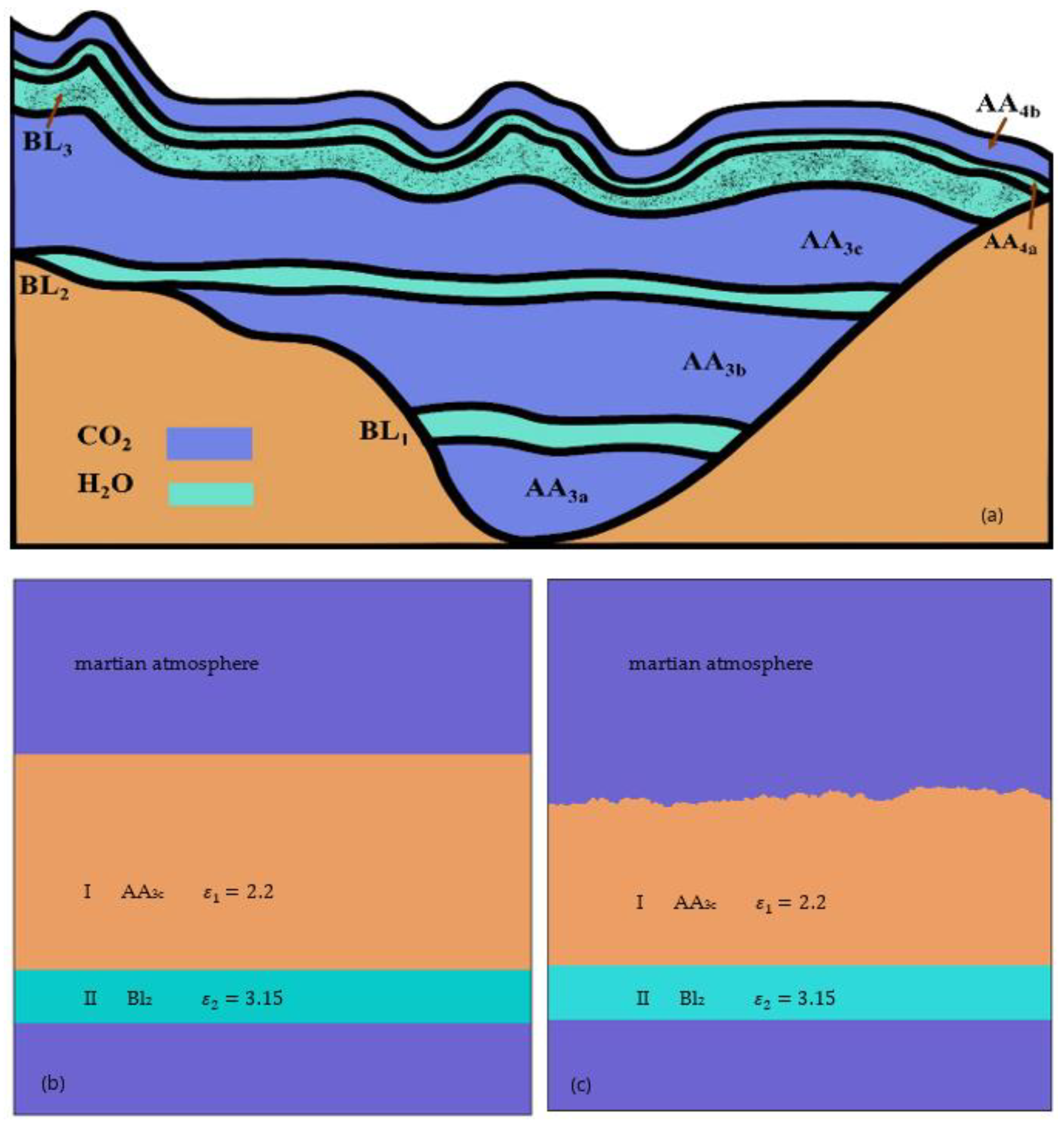
2.1. Stratigraphy of Martian South Polar Ice Cap

From top to bottom, seasonal frost, the SPRC, and the SPLD compose the Martian south polar ice cap [2]. The thickness of the seasonal frost composed of dry ice (CO₂) is less than 1 m, whereas the residual cap is formed by an ~8 m thick CO₂-dominated layer and a thin water-ice basal layer [1]. The late-Amazonian sedimentary layer of the south polar plateau can be divided into Planum Australe 1 to 4, or AA_1–4 [2]. The AA₄ unit delineates the residual ice cap. SPLD is comprised of water-ice deposits, mixed with different levels of dust, and includes units AA_1–3 [2]. The AA₃ unit is ~300 m thick and appears to be limited to the summit area. It can be further divided into up to three CO₂ layers (AA_3c-a), each capped by thin H₂O layers (BL_3–1) [8,9]. Figure 1a shows the profile of units AA_3a to AA_4b. However, the AA₄ or the uppermost surface cannot be observed by SHARAD because its thickness is lower than the vertical resolution of SHARAD, which is ~11 m in water ice [8].

The AA₂ unit underlying AA₃ consists of evenly bedded planar sequences, and unconformably overlies most surfaces of unit AA1, which is the main component of SPLD with maximum thicknesses of >3.5 km. The layering structure revealed by SHARAD is suggestive of the erosion and deposition of Martian polar ice caps that interacted with mid-latitude sediments [10,11], which are accompanied by unconformable contacts between different units.

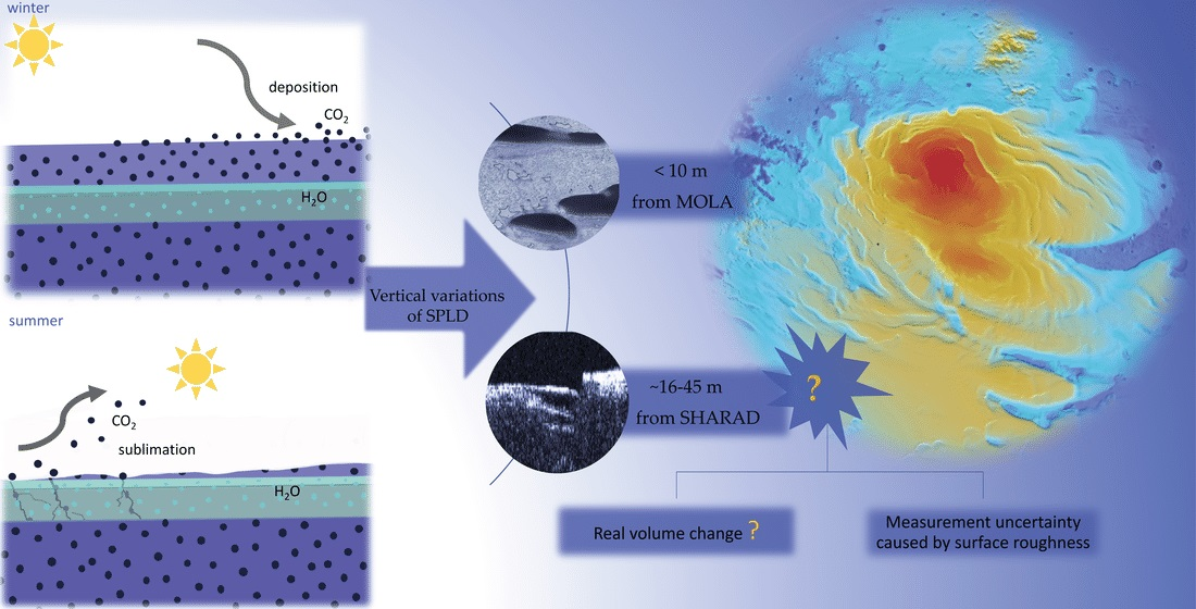
2.2. Temporal Variations of South Polar Cap

The Martian atmospheric pressure has seasonal and periodic changes due to the removal and deposition of the seasonal ice cap [12]. The CO₂ deposits on the surface become thicker and thinner due to frost in winter and sublimation in summer, respectively [13]. CO₂ frost reaches maximum accumulation at solar longitude, Ls = 155°. The solar longitude (Ls) is the Mars–Sun angle, and for the southern hemisphere, the autumn equinox is Ls = 0°, followed by the winter solstice at Ls = 90°, spring equinox at Ls = 180° and southern summer equinox at Ls = 270°. MOLA data indicate that the seasonal variation of surface elevation predominantly causes the seasonal cycle of CO₂ condensation and sublimation to be less than 1 m [14,15]. Generally, the SPRC has been balanced with the atmosphere, so it is sensitive to changes in the Martian climate [12,16]. Its temporal variations can be observed from MRO Context Camera (CTX) images, which provide context with ~6 m/pixel resolution. The quasi-circular depressions known as “Swiss Cheese” [1] features appear on the surface of SPRC (Figure 2a). In the summer when CO₂ frost is removed, the walls of the depressions composed by an 8 m thick CO₂-ice layer expand outward with a constant erosion rate [17], as shown in Figure 2b,c. Based on the observed erosion rates and the size of the erosion pits, studies estimated that SPRC has existed on Mars for a century [17,18]. The area of SPRC did not fluctuate significantly during the long period of erosions of pits and slopes [19,20].

Sublimation and erosion also occur in the AA₃ unit. The polygonal patterns formed by highly fractured water-ice layer BL₃ are unique features found at the surface of AA₃, which might allow the buried CO₂ ice to volatilize and form depressions. The troughs, depressions, and pits observed in the AA₃ unit have a depth of ~75 m, indicating that some areas have internal CO₂ volatilization and release [9]. SHARAD observations at different times can help us understand the temporal variation of the AA₄ and AA₃ units.

3. Materials and Methods

3.1. Data

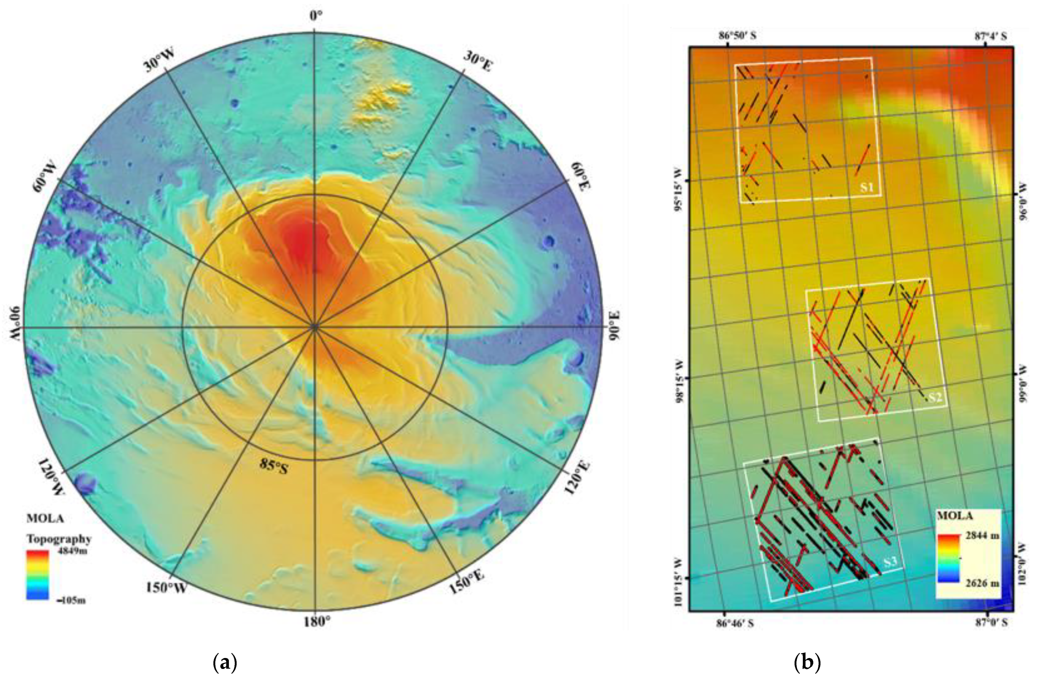
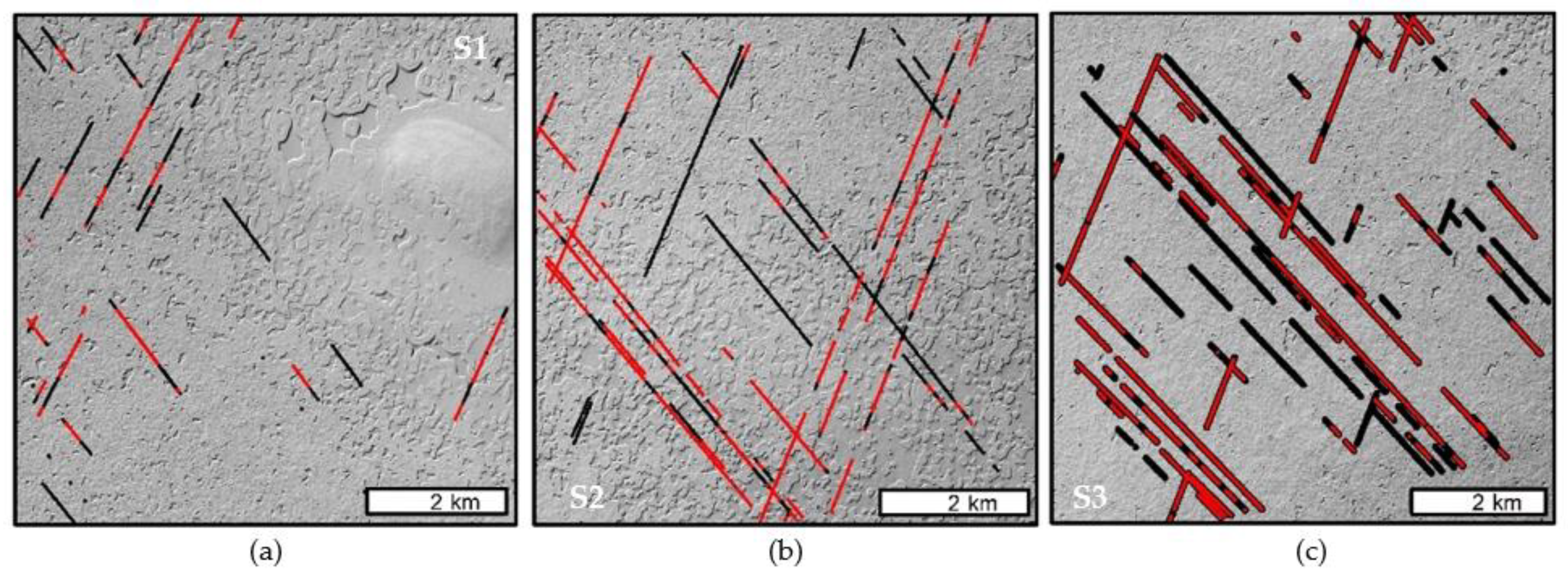
3.1.1. Study Regions

Three study regions indicated by the white squares in Figure 3a were determined based on two criteria. The first criterion was to select the region containing subsurface CO₂ deposits within unit AA₃. Its layering structure can be clearly observed in radargram. The AA₃ unit overlaps the AA₄ horizontally [9] in several instances. Therefore, we selected S1–S3 in Figure 3b as our study area, which is mainly located at 93°–101°W in longitude, 86°46′30″–87°02′30″S in latitude and is ~108 km² in total area. The side length of the three regions is ~6 km, respectively. Each region is within the horizontal resolution of SHARAD to obtain the time difference of the layer thickness at the same location. The parameters on SHARAD will be described in 2.1.2. The second criterion was to select SHARAD data with clear horizontal reflectors, so an area with a smooth surface was selected to minimize the measuring uncertainties of layer thickness caused by roughness. Figure 4 shows the CTX images of three study areas mainly located on the geologic units B6 and B7, where eroded landforms such as 2 m sized pits are commonly seen. The erosion features in B7 are mostly isolated mesas and low scarps, with few remaining pits, so surface roughness has little impact on radar signal in this area. In this region, surface clutter is barely seen, providing a clear view of surface and subsurface echoes used for data analysis. S2 belongs to B6 [21], the surface of which is coarser than those of S1 and S3 (Figure 4), with numerous pits of a depth of ~2 m [21]. The smooth surface of S1 and S3 has an advantage for improving the accuracy of the layer thickness, as measurement uncertainties are sensitive to roughness, and temporal variations are close to SHARAD resolution.

3.1.2. Shallow Radar Data

SHARAD instrument carried by the MRO began to work in October 2006, collecting radar echoes reflected from the Martian surface and subsurface layers. Its frequency is 15–25 MHz, and its bandwidth is 10 MHz. SHARAD can penetrate about 1 km beneath the Martian surface [8]. The vertical resolution of SHARAD in the subsurface layer can reach 10 m to 20 m [9] and has a cross-track resolution of 3–6 km and an along-track resolution of 0.3–1 km [3].

More than 6000 data points from SHARAD have been viewed for this study area. These cover Martian years 28–34, or an observation period from 2007 to 2018. The red dots in Figure 4 show the 4862 points with clear surface and subsurface echoes, which were selected for analysis. A rough surface could cause the delay offset and increase the half-height width of SHARAD echoes. To reduce the influence of roughness on the data uncertainties, we set the upper threshold value of FWHM (full width at half maximum) to filter radar data. In this step, the radar echo trace of each subsatellite point was extracted and the corresponding pulse width measured. Data points, both surface and subsurface echoes of which have a pulse width of less than 150 ns, were used for subsequent statistical analysis. Figure 5 illustrates the depth of subsurface echo from the bottom of the AA_3c and the pulse width before and after filtering.

3.2. Methods

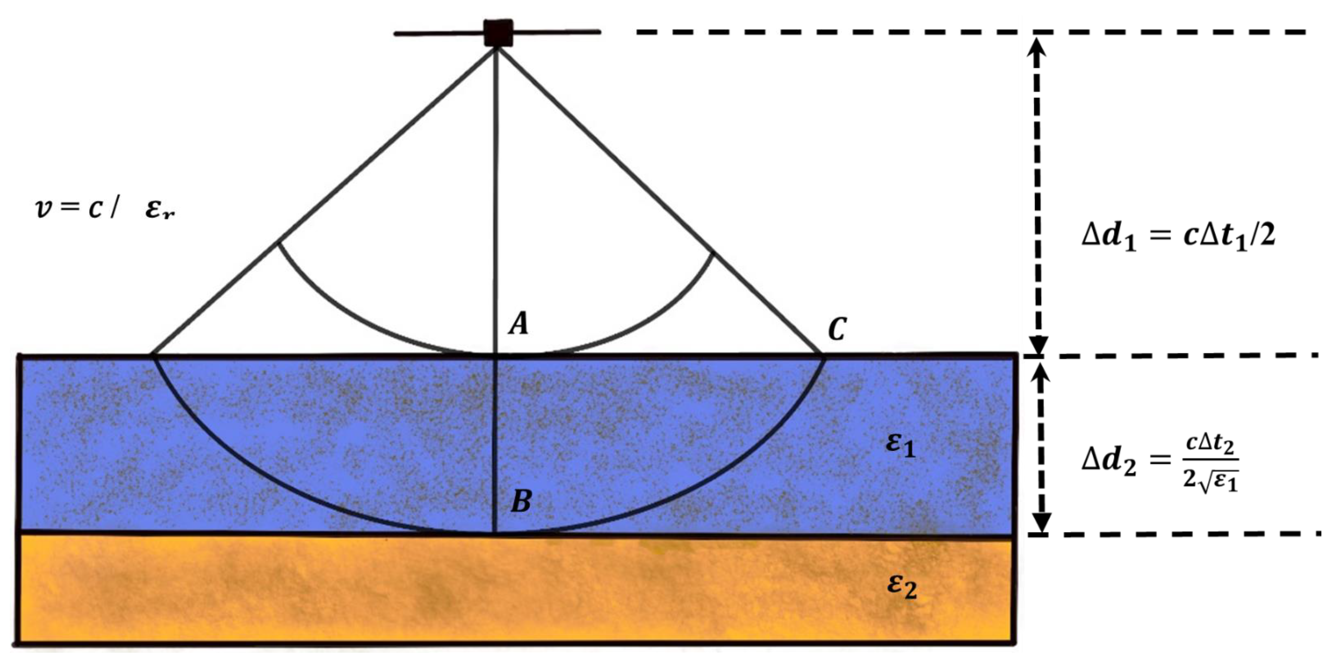
3.2.1. Measurement of CO₂ Deposits’ Thickness

The thickness measurement is illustrated in Figure 6. When electromagnetic waves emitted by the radar enter the Martian crust, the speed of propagation in the first layer v is reduced relative to the vacuum, here $v=c/n$. n is the refractive index of the medium, associated with the real part of the dielectric constant ${\epsilon }_r$,$n=\sqrt{{\epsilon }_r}$. If a subsurface layer with a discontinuous dielectric constant is present at a depth ∆d₂ below the surface layer, the reflection and transmission of electromagnetic waves will occur again at the interface.

The secondary reflection echo penetrates layer one and should be received by the radar, although the signal is much weaker than the surface echo. The time delay ∆t₂ between the subsurface echo and surface echo can be used to calculate the thickness of layer one ∆d₂$=c∆t_2/2\sqrt{{\epsilon }_1}$(Figure 6).

Suppose that the surface of Mars is smooth and flat, only echoes of sub-satellite nadir point A can be received. However, in a real case, radar might also receive the reflection from C on the surface (Figure 6). If its time delay is the same as the echo of the subsatellite point on the subsurface B, then it is likely to submerge the signal of B, which brings the problem of clutter. Clutter simulation, which uses a digital elevation model (DEM) to model the reflections from the non-nadir surface, is necessary to identify the subsurface echo. Figure 1a shows the stratigraphic map in the study areas. Since the thickness of surface layer AA₄ is about 10 m, less than the vertical resolution of SHARAD, the lower interface of AA₄ cannot be clearly seen in radargram. Therefore, the first layer recognized in the radargram includes AA₄ if present, Bl₃, and AA_3c, meaning the measurement results given in this work are the overall thickness of three sublayers. For convenience, we call the first layers AA_3c. We took the dielectric constant of 2.2, a typical value for the mixture of water ice and dry ice. The temporal change of thickness within seven Martian years in each small area was calculated and is shown in the results section.

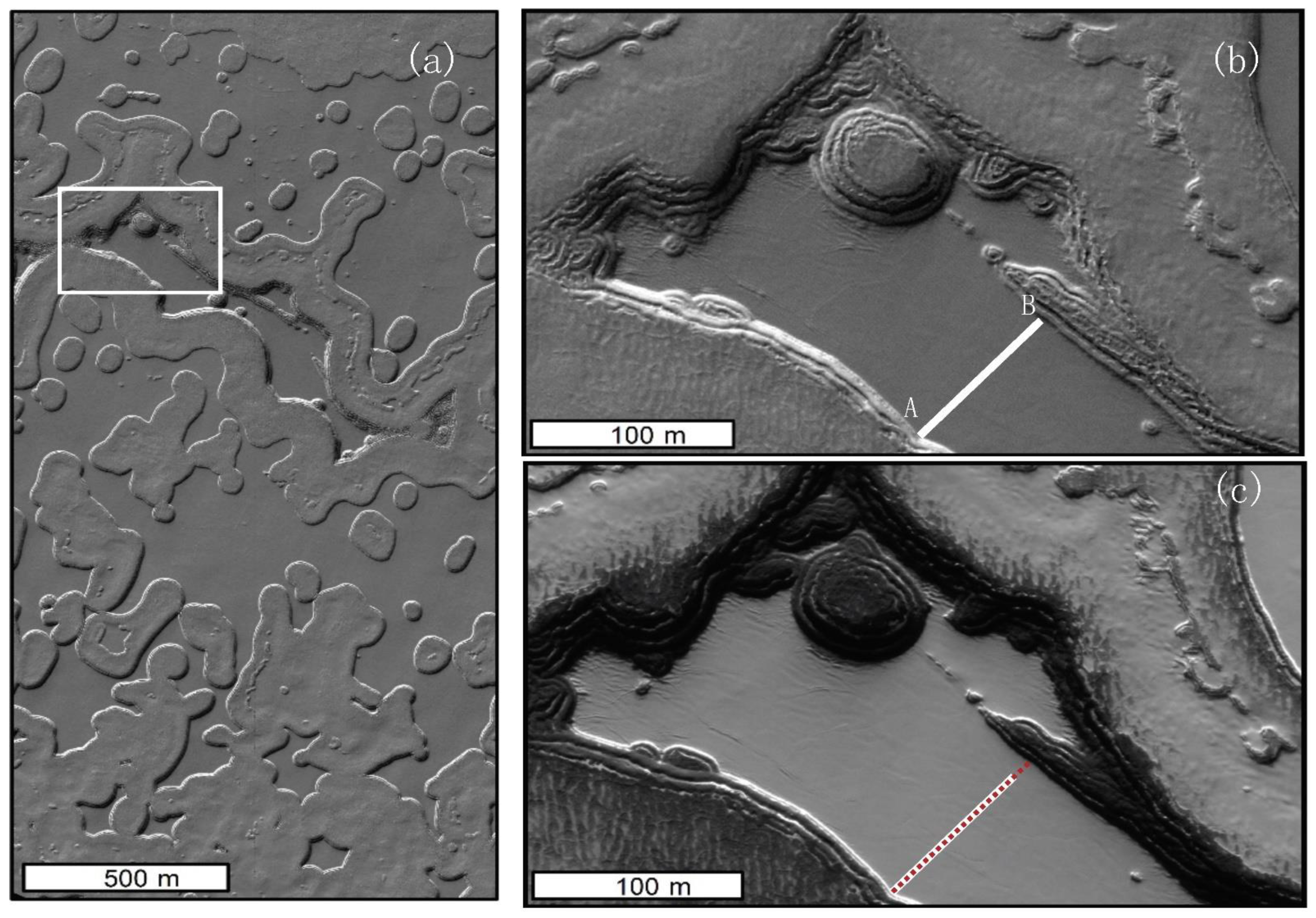
3.2.2. Surface Roughness

To analyze the influence of surface roughness on uncertainties of measurements, we performed the simulation of radar signals with two models. GprMax, a software based on the finite-difference time-domain (FDTD) method [22] to model ground-penetrating radar (GPR) responses from arbitrarily complex targets was used in this study. Two-layer models were established, as illustrated by Figure 7. The first layer represents the model of AA_4b, AA_4a, Bl₃, and AA_3c layers. The dielectric constant of AA_3c is in the range of 2.0 to 2.2 [9] and in this paper the average of these layers ${\epsilon }_1=2.2 \mathrm{is}\mathrm{used}.$ The second layer models Bl₂, nearly pure water ice,${\epsilon }_2=3.15$ [8,9]. In the smooth surface model, the thickness of the first layer is 325 m, and the thickness of the second layer of water ice is 50 m. According to the observation results of SHARAD, the thickness difference between winter and summer is in the 0–45 m range, and the specific description is in 3.1.1. Therefore, the elevation of the rough surface is lower than that of the smooth model surface. The simulation results of a smooth surface (Figure 1b) and a rough surface (Figure 1c) are compared to show the influence of surface roughness on radar signals.

The surface roughness is calculated with Equation (1). This parameter can reflect the elevation change of each vertex of the surface cell grid in the analysis area. The value from elevation data is highly correlated with the clutter of the SHARAD profile [23].

Roughness = Root mean square elevation/Average elevation

(1)

The elevation data in the study region were generated with CTX image pairs and the NASA Ames Stereo Pipeline (ASP) tool [24], and the resolution is 18 m/grid point [25]. Although a DEM model derived from HiRISE data is more accurate and trusted in estimating the influence of seasonal variations of surface roughness from SHARAD radar signal [26], the best available DEM model in the study area we obtained was developed from CTX images, which also shows clear changes of geomorphology in different seasons.

4. Results

4.1. Seasonal Variations

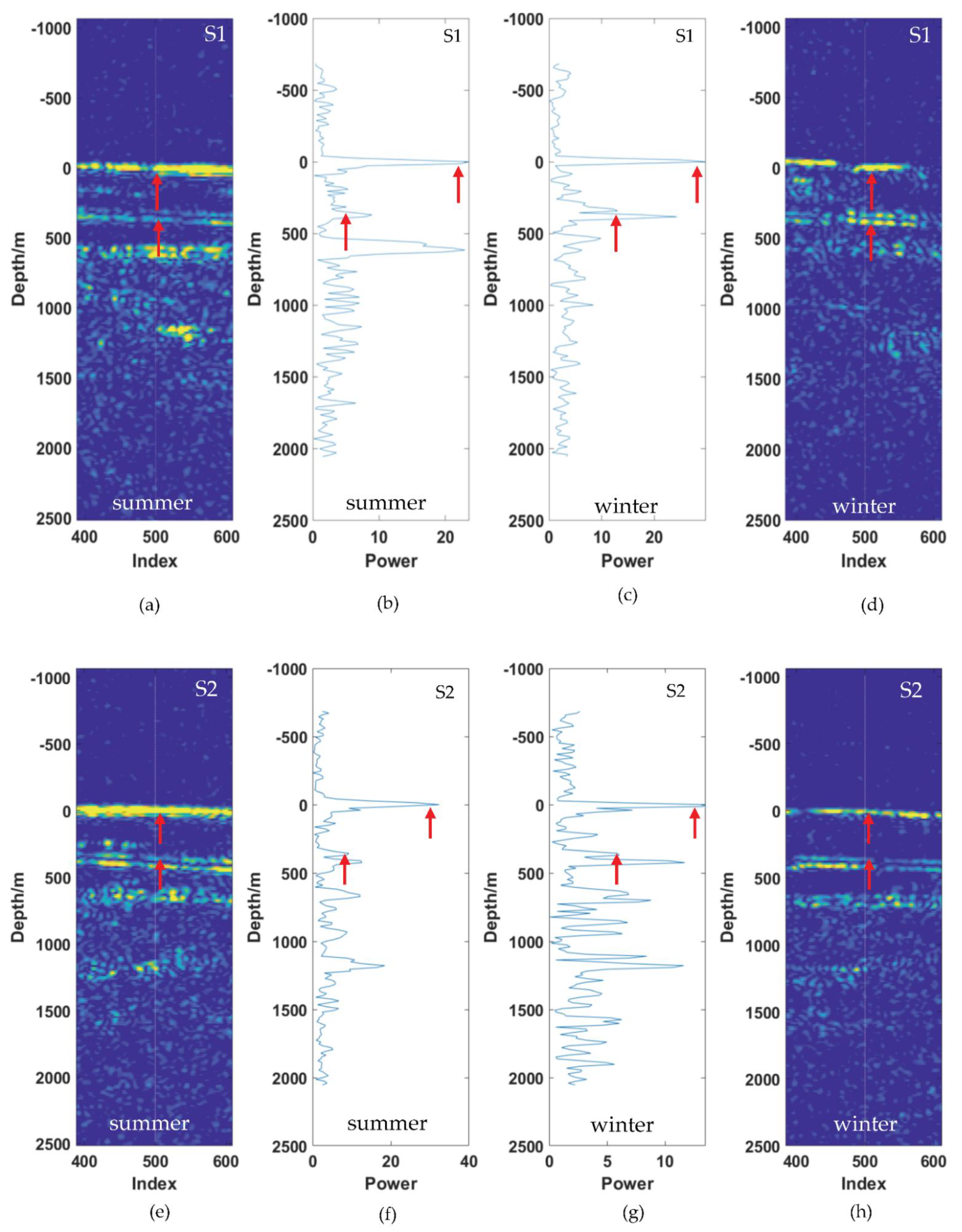
4.1.1. Case Studies of Seasonal Variations

Previous studies show that seasonal variations and yearly erosions occur on the AA₄ layer, and the CO₂-ice layer of AA_3c might sublimate through the cracks of AA_4a in summer and lead to a collapse in some areas [9]. To obtain the temporal variation of the same layer, we select one point pair with a subsatellite distance of less than 3 km. The radar profile of each point provides the positions of the surface and lower interface of AA_3c, and then the thickness can be obtained. The seasonal variation is estimated by comparing the thickness at different seasons, e.g., thickness in summer and winter. Figure 7 presents two comparison cases of radar profiles in different seasons.

The frosts on the surface sublimate in summer and are deposited in winter at the south pole. The surface roughness is usually higher in summer than in winter. In addition, AA_4b is eroded at a constant rate by expanding outwards from the steeply sided walls of the depressions, and the AA_3c unit might sublimate through the cracked BL₃ layer in the spring and summer. In the radargram from Figure 7, the surface radar reflections appear wider, and clutter is more abundant in summer than in winter, causing uncertainties in measuring the thickness. Another prominent phenomenon caused by seasonal change is that the subsurface echo also becomes wider and fuzzier in the summer, leading to measurement errors. The “foggy” signals appear at depth in the summer radargram of Figure 7a, resulting in difficulties in identifying other AA₃ subunits. The causes of “foggy” echoes, whether they are formed due to surface roughness or are also related to subsurface roughness, e.g., sublimation of the AA₃ layer, are analyzed with the simulation results (details in Section 3.2.2). In Figure 7d, although echoes of the surface and the upper interface of AA_3c are sharper than those in the summer season, the lower interface of AA_3b in the winter disappears in both the radargram and radar single trace profile.

Table 3. Six cases of SHARAD observations in different Martian seasons. Ls: solar longitude; Depth: the position of the lower interface of AA_3c; Distance: subsatellite distance between two nodes.

Cases	Study Area	Ls (degree)	Depth (m)	Δd (m)	Distance (m)
1	s1	328	348.90	45.51	1026.29
		102	394.41
2	s1	309	348.90	15.17	2526.43
		102	364.06
3	s1	309	348.90	45.51	2053.82
		92	394.41
4	s2	328	364.06	30.34	2296.63
		148	394.41
5	s2	328	364.06	45.51	2542.52
		148	409.57
6	s2	328	394.41	15.17	2807.44
		148	409.57

lists six data pairs of SHARAD for observations of seasonal thickness variations in S1 and S2.

Table 1. The thickness measurement in S1. Ls: solar longitude; WS: FWHM of radar echo on the surface; Depth: the depth of the lower interface of AA_3c; Δd: the thickness difference of AA_3c in the two different seasons; Δw: the pulse-width difference of surface echo in the two different seasons. The data points correspond to Figure 7a–d, track numbers are 0564201 and 3577202.

Study Area	Ls (Degree)	Depth (m)	WS (ns)	Δd (m)	Δw (ns)
S1	309.4	348.8	138.6	30.4	−23.3
	92.0	379.2	115.3

shows that the thickness of the AA₃ layer does have seasonal variations ranging from ~16–45 m, which could reach 3 times the vertical resolution of SHARAD data.

The results given in Table 1 and

Table 2. The thickness measurement in S2. Ls: solar longitude; WS: FWHM of radar echo on the surface, Depth: the depth of the lower interface of AA_3c, Δd: the thickness difference of AA_3c in the two different seasons; Δw: the pulse-width difference of surface echo in the two different seasons. The data points correspond to Figure 7e–h; track numbers are 0564201 and 1056001.

Study Area	Ls (Degree)	Depth (m)	WS (ns)	Δd (m)	Δw (ns)
S2	328.1	394.4	144.3	15.2	−23.7
	148.2	409.6	120.7

indicate that the thickness of shallow deposits in winter is higher than that in summer, and the FWHM of surface layers in summer increases by ~20% compared to winter.

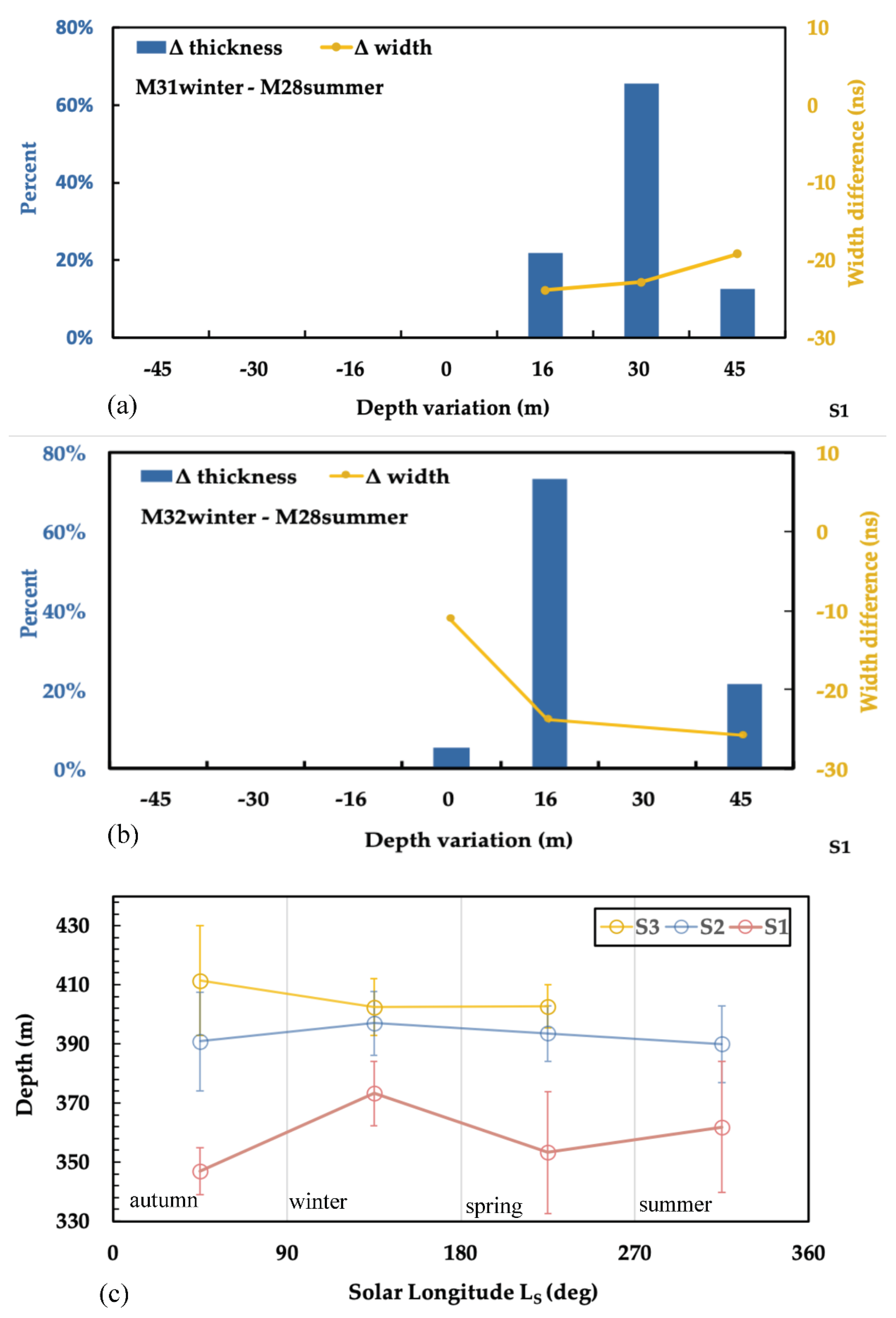
4.1.2. Statistical Study of Seasonal Variations

Through the SHARAD observations of 11 terrestrial years from May 2007 to September 2018, we can see some variations in the thickness of AA_3c during different seasons based on the statistical analysis of these track intersections in S1, S2, and S3.

From M28 in summer to M31 or M32 in winter, most AA₃ layers have a positive change in thickness, ~16 m to 45 m in S1, as shown in Figure 8a,b. In the studied S1 region, the majority of the thickness variation is larger than the SHARAD vertical resolution, and a few of them reach three times the resolution. As we expected, the pulse width of the surface echo in winter is narrower than that in summer, meaning their differences are all below 0. We speculate that a layer variation larger than the MOLA observation might be caused by surface roughness. However, no clear correlation between the width variation and thickness variation is observed from Figure 9, which means that the large change of surface roughness does not correspond to a large thickness variation.

Figure 8c shows the average thickness of shallow deposits in each season in S1, S2, and S3. We found that the thickness of each region in the winter is greater than that in the summer, which is consistent with previous case studies. The range of the average thickness variation is from ~7 m to 20 m, higher than prior studies [15] which reported ~1 m of seasonal variation on the surface AA₄ layer. The error is calculated from the standard deviation, whose range is ~9–21 m. The error in winter is relatively smaller than in others, and may be due to the stable data quality on the smooth surface in winter. The source of the measured thickness is difficult to model as it represents a comprehensive change of multiple deposition layers: AA_4b, Bl₃, or AA_3c. In addition, the uncertainties of the measurements, especially the influences of surface and subsurface roughness, should be considered to obtain the quantity of the temporal variations of the shallow deposits in the south polar region.

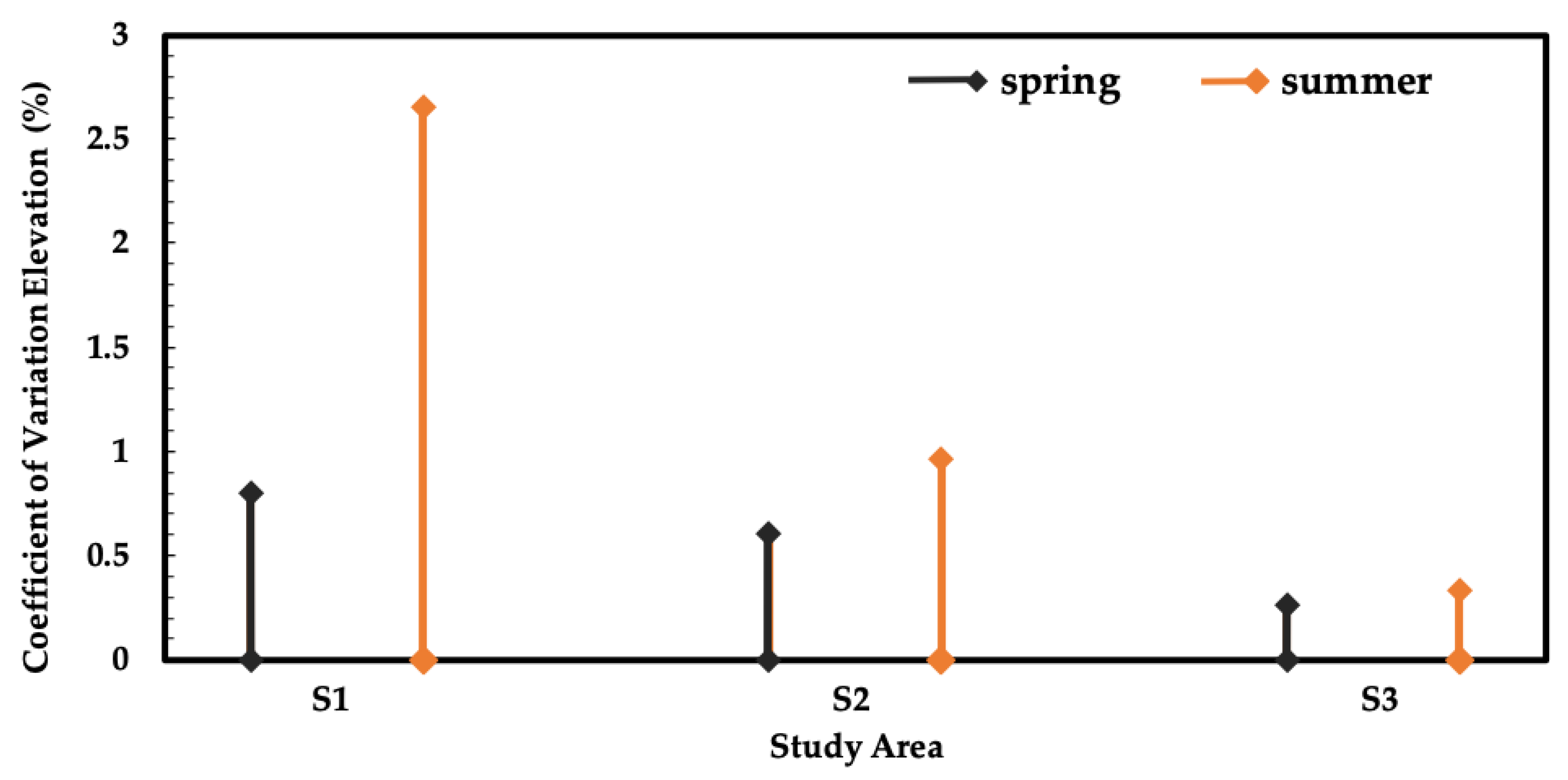
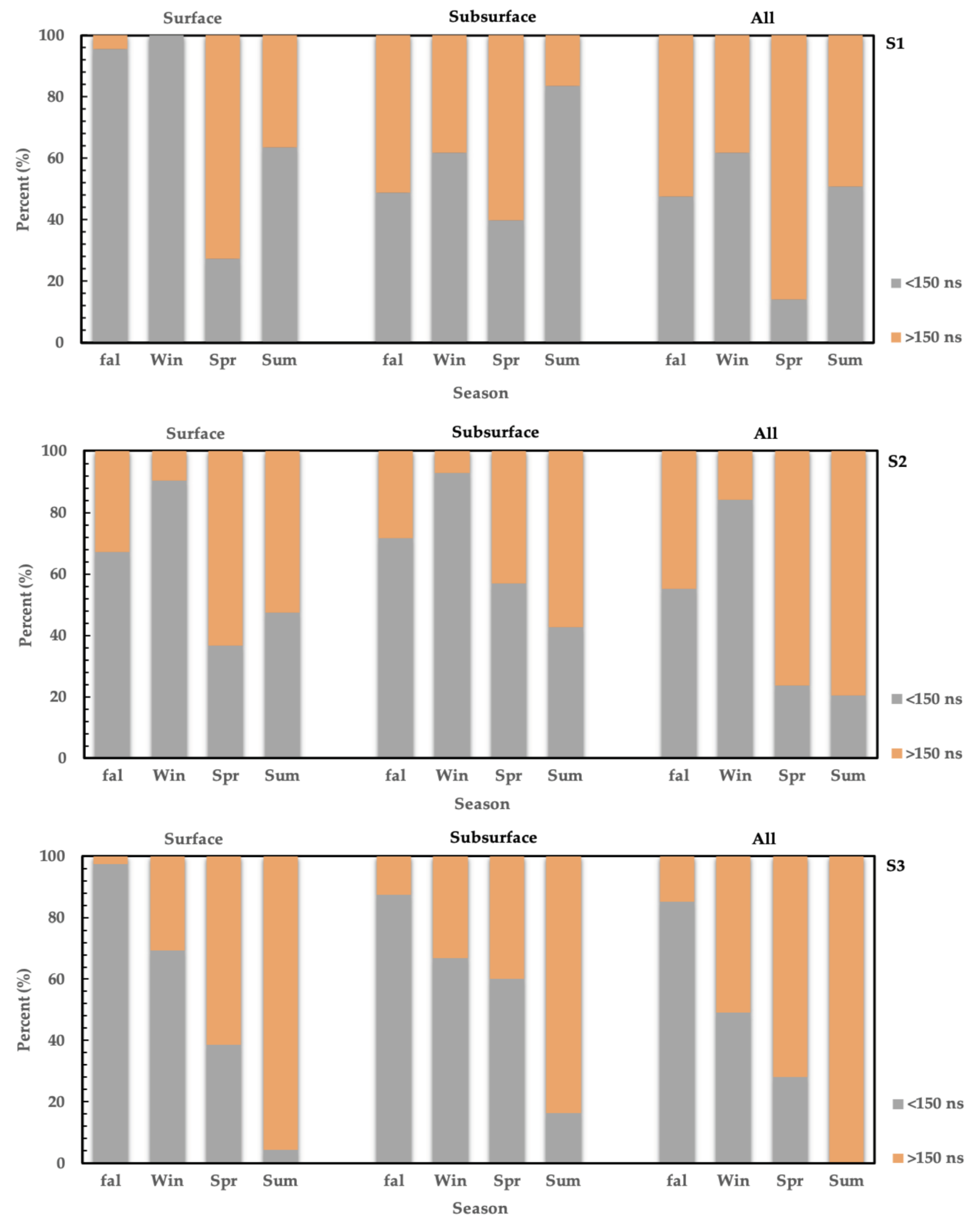
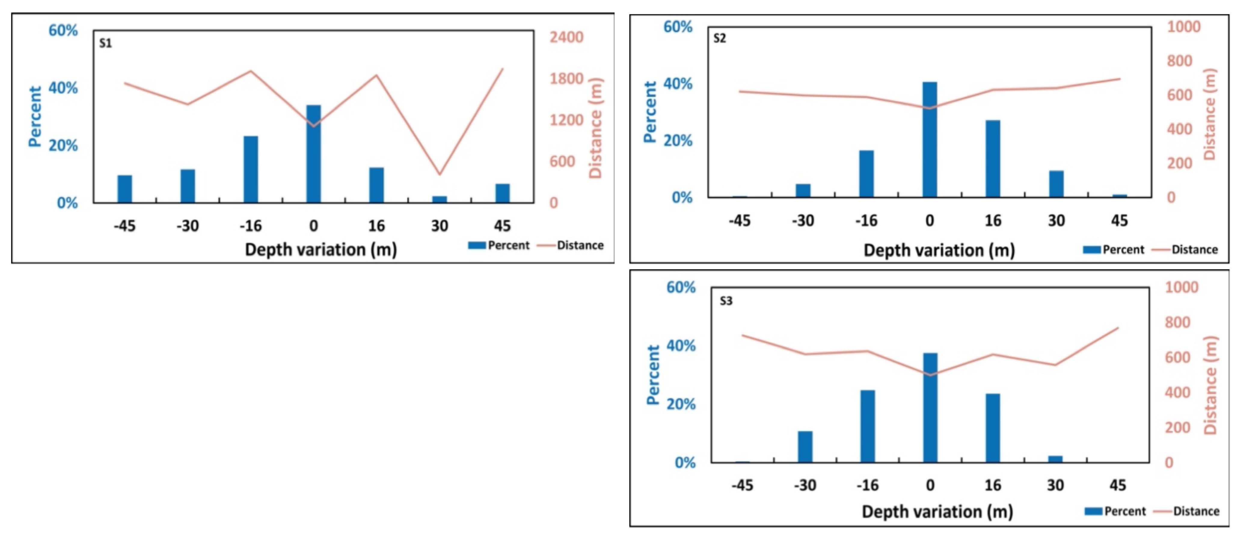
4.1.3. Seasonal Variations of Surface Roughness

The temporal variations of the thickness measured by SHARAD could be affected by the seasonal changes of surface roughness.

Table 4. The maximum value (MAX) of the roughness in the summer/spring season of study regions. The elevation data were generated with CTX image pairs, the indices of which are listed in Supplementary Table S1.

Region	Index	Ls (Degree)	MAX (%)
S1	1	228	0.8
	2	318	2.8
	3	318	2.5
S2	1	204	0.8
	2	228	0.5
	3	288	2.2
	4	286	1.0
	5	318	1.0
	6	310	0.8
	7	325	0.6
	8	326	0.5
	9	335	0.7
S3	1	204	0.3
	2	286	0.5
	3	337	0.2

lists the maximum value of the surface roughness obtained with Equation (1) and elevation data using CTX image pairs. Figure 9 shows the average maximum surface roughness and corresponding season in S1, S2, and S3. Due to the lack of winter/fall CTX stereo images in the study region, only the roughness data in the summer/spring seasons were analyzed. Based on Table 4 and Figure 9, we can conclude that the surface roughness in summer is greater than that in the spring, especially in S1, where the difference could reach 5%. This is because the surface dry-ice layer (AA_4b) begins to sublimate in spring, and then later in the summer, more surface CO₂ sublimates to the atmosphere and the rough surface is exposed.

To find the relationship between the surface roughness and the radar signal, we performed a statistical analysis on the 3 dB pulse width of surface echoes. Figure 10 shows the statistic study of all the data including those with FWHM greater than 150 ns. For the data points with FWHM larger than 150 ns, the numbers of autumn points and winter points account for more than 60% of the total data, while for the data points with FWHM smaller than 150 ns, data of spring and summer seasons have a larger proportion. This seems due to the fact that the increased width of the radar signal is caused by the rough surface in the summer. The pulse width of the subsurface shows a similar pattern, with the exception of S1. From these results, the width of the surface/subsurface echo of the radar has seasonal variations and is related to the seasonal change of the surface roughness.

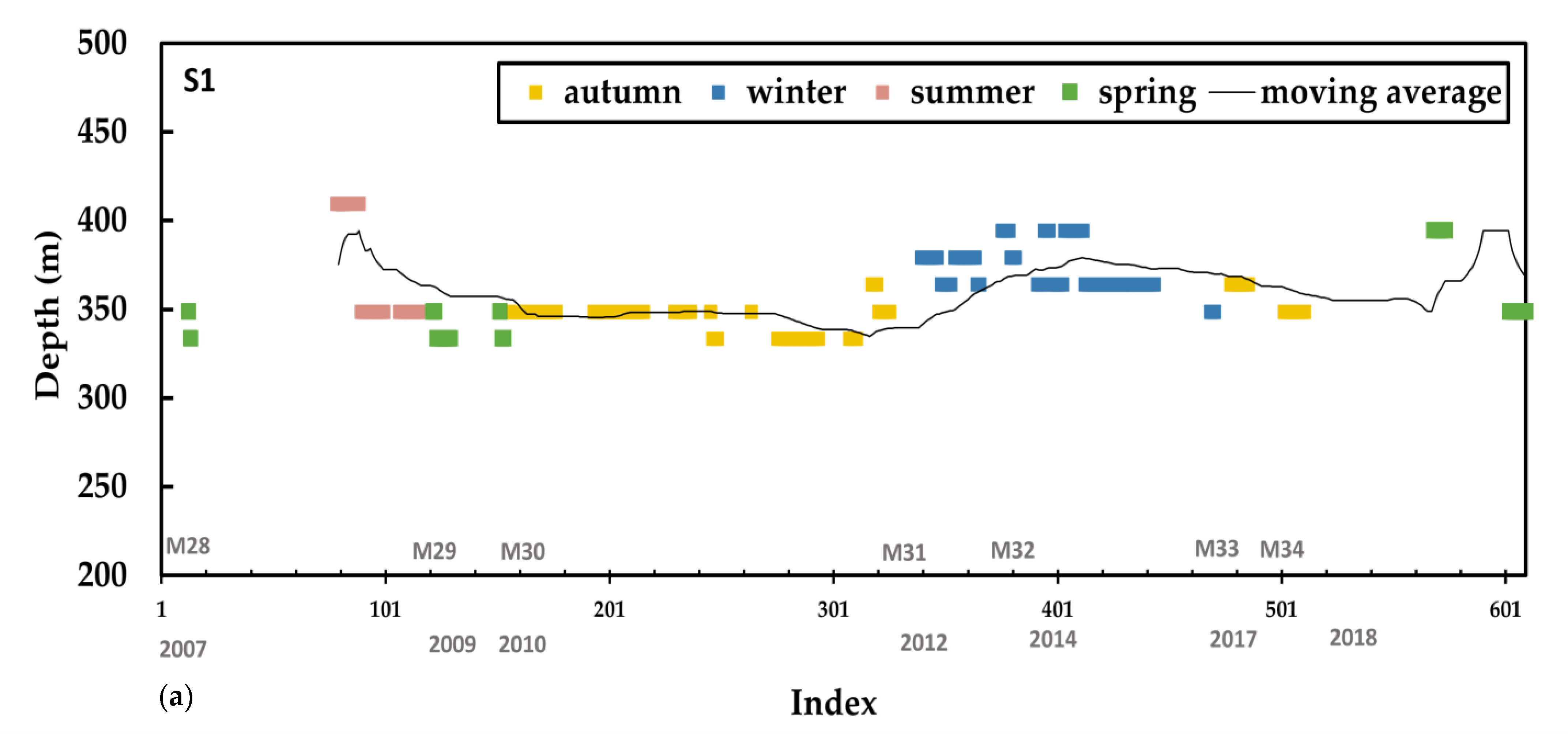
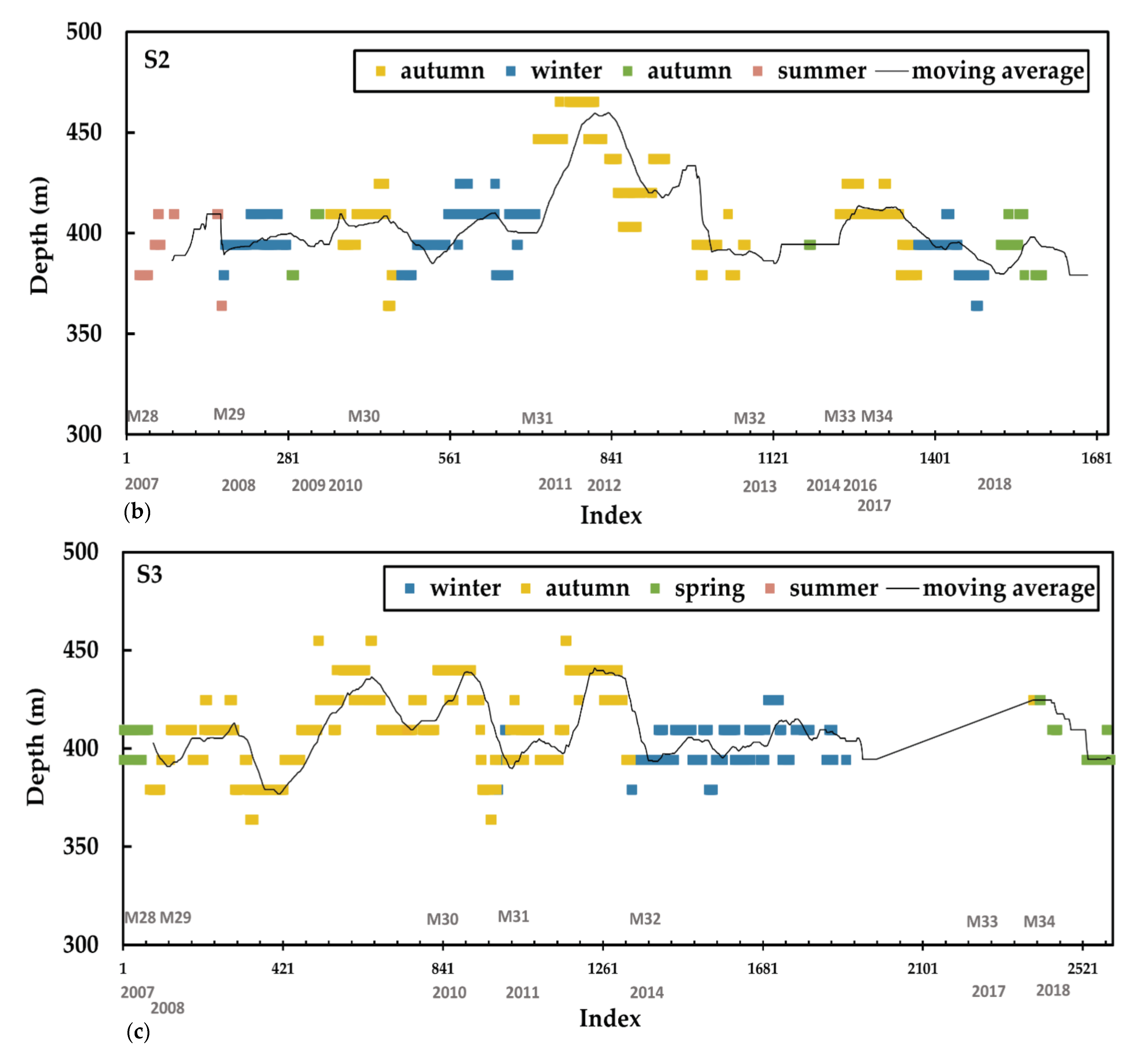
4.2. Variations of CO₂ Layer Thickness in 11 Terrestrial Years

Figure 11 shows the thickness variations of shallow deposits at all subsatellite points with the observation period in the three study areas. The thickness values span multiple levels with the fixed gap determined by radar data-sampling rate. Although the thickness of AA_3c has periodic variations, it did not show an obvious increasing or decreasing trend during these 11 terrestrial years from the moving average. The reason could be that the slight yearly change of the thickness is not detectable by SHARAD.

Another observation from Figure 11 is that in the same area, the thickness of AA_3c has been constantly fluctuating in value. It raises a reasonable suspicion that thickness variation is mainly due to regional differences of two compared data points. To find out the possible cause, we show the distribution of the thickness value and the corresponding average subsatellite distance between the data pair in Figure 12. The statistical results display a normal distribution of temporal variations of CO₂ ice in S1, S2, and S3. We expect that the average distance increases with the thickness variations, as it is likely the two points further apart have large variations in the AA_3c layer thickness. However, such correlation between thickness variations and the average distance is not very clear in Figure 12. The systematic variations of thickness may not be the main reason and we could not exclude the possibilities that observed variations are caused by measurement errors such as low radar resolution and the influence of surface roughness. To evaluate the latter, a simulation of the radar signal was performed, and the results are given in the following subsection.

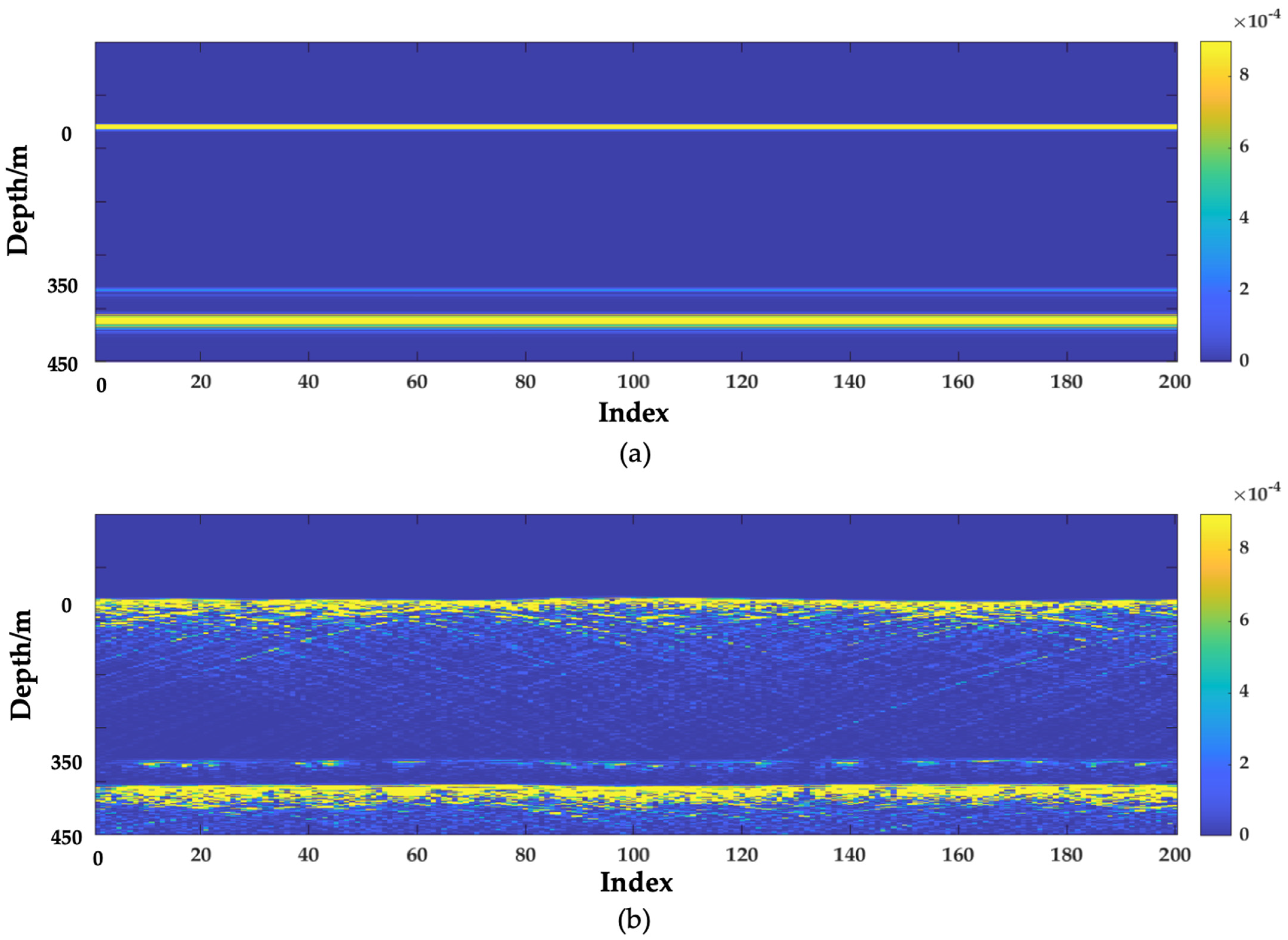
4.3. Simulation Results of Rough Surface

From the results of the surface roughness simulation on the radar signal, the surface echo of the smooth surface (Figure 13a) is clear and sharp, and the position of the surface echo can be accurately determined. When the surface roughness increases (Figure 13b), the width of the surface echo also increases significantly, and the width can reach ~30 m at the widest point. We believe that the increase in surface roughness results in a rich surface echo signal and the appearance of signal superimposition, which causes errors regarding the position of the surface echo, thereby affecting the accuracy of measurement on the thickness of AA_3c. The simulation results show that the surface roughness does affect the measurement of layer thickness by increasing the width of surface and subsurface echoes. In addition, not only is the surface echo affected by the roughness, but the subsurface interface in the radargram becomes wider and rougher, which contributes further to the uncertainties of the measurement. It also indicates that the blurred subsurface boundary in the summer may not be caused by the rough subsurface but by the sublimation of the surface CO₂ layer.

5. Discussion

With 11 terrestrial years of observation data, we found that the thickness of the AA_3c layer (which also includes surface AA₄ layer if present) is essentially between 300 m to 400 m, and the layer of the thin water ice between AA_3c and AA_3b, or Bl₂, is mainly 30 m to 60 m thick. There are two—or even three—layers of CO₂ ice in some regions, and each CO₂-ice layer is separated by a thin layer of water ice. This observation was consistent with previous research results. The diagram of the stratigraphic structure of AA₃ is shown in Figure 1, which is drawn based on the SHARAD radargram (Figure 7). The underground layered sediment measured in this work includes AA_4b, AA_4a, Bl₃, and AA_3c layers.

Through measuring the thickness variations of AA_3c, the results in Section 3.1 show that there is indeed a seasonal thickness difference, meaning that the thickness of the AA_3c layer in the same location may vary in different Martian seasons. From the results, we found that the thickness of the shallow deposits thickens in winter; consequently, the dry-ice layers decrease in the summer. The maximum variation value is about three times of SHARAD resolution; hence, it is unlikely that the observed seasonal variations are random noises due to detection limitations. In addition, this phenomenon is not caused by regional factors as shown in Figure 12.

The previous study shows that seasonal sublimation and deposition of dry ice occurs on the surface near the Martian southern polar ice sheet. However, the change in the surface dry ice measured with MOLA data is within 10 m, and most is concentrated in 1 m [15], much lower than the upper bound of results given by SHARAD observations. The internal dry-ice layer can be sealed by a ~15–45 m thick water-ice layer [8] and may sublimate in the spring or summer if there are cracks on the surface [8,9]. Unfortunately, we did not observe any cracks on AA₄ in our study area at present. A conceptual model was proposed that the subsurface dry ice sublimates in the event of no gaps being on the surface in the northern polar cap. The sunlight shines through the water ice into the lower layer of dry ice, and the dry ice sublimates until the pressure is large enough to break the thin upper layer of water ice [27]. According to this model, if the water ice of the upper layer is brittle, then the AA_3c can escape. In late spring, the dry-ice layer of the seasonal ice cap was evaporated, and then the lower layer of water ice or Bl₃ will be exposed. When the summer comes, sunlight will penetrate the water-ice layer, and it is possible that the AA_3c sublimates in the same way to form cracks on the overlying layer. Eventually, the underlying dry ice will reduce, and the surface water-ice layer will collapse. However, even if the internal dry ice in the study area escapes, can the total thickness variation of the shallow deposits reach tens of meters?

To investigate whether the SHARAD observation data reflect the real volume change or are caused by uncertainties of measurement, we conducted roughness analysis on the elevation data in different seasons and found that roughness in summer is greater than that in spring. At the same time, we observed that the FWHM is wider in the summer than that in other seasons. From the consistency of the variation for signal width on the surface and thickness of dry ice, we suspect that the surface roughness will lead to the broadening of the width of radar signals and an increase in errors of measurement. Specifically, it is the surface roughness which affects the width of the radar’s echo signal, which in turn affects the position of the echo, and finally results in a difference in layer thickness. The simulation results also demonstrate that the surface roughness can also affect the width of subsurface echoes, which further contributes to the deviation of the measurements. Therefore, the resolution of SHARAD is not high enough to quantify the vertical changes of the thickness of shallow deposits within the geologically short period.

The variation in mass for the dry ice buried in the south pole of Mars is closely related to the history of the Martian climate’s evolution. The intersection of every two tracks was used to extract the subsatellite points of different years in the same area for our comparative analysis. In the 11 terrestrial years from 2007 to 2018, the thickness of the shallow dry-ice layer, or AA_3c, has had no obvious trend of thickening or thinning. It is currently believed that although the layer of dry ice may experience erosion, the variations during a geologically short period are not detectable by SHARAD. In the future, an instrument with high vertical resolution can provide more data on the elevation changes of SPLD for the modeling of the evolution of the Martian atmosphere.

6. Conclusions

The sediments in the polar regions of Mars carry a record of its past climate. Imagery and spectrum data can be used to assess annual changes in the lateral coverage of volatile deposits. However, vertical variations, in particular the changes of the buried CO₂-ice layer, cannot be assessed this way.

In this work, we used data from the SHARAD, which has been measuring the Martian stratigraphy since 2007, to obtain temporal variations of the shallow deposits in the south polar region. Analyzing the data produced through different seasons during seven successive Martian years in the region of interest, we have observed strong seasonal variations showing that shallow deposits are thicker in the winter than in the summer. However, the maximum variation values are much higher than found in previous estimations based on MOLA data. The reason could be the measurement uncertainties introduced by variations in the surface roughness, as this work shows that there is a correlation between the seasonal changes of surface roughness, calculated with the elevation data generated with CTX image pairs, and the width of the surface radar echoes. In addition, the simulation results suggest that the subsurface radar echoes are also affected by the surface roughness, leading to further measurement deviations. SHARAD was thus successful in detecting clear seasonal variation of the southern polar deposits, but its limited resolution and influences of surface roughness make it difficult to derive quantitative vertical variations within a short geologic time. In the 11 terrestrial years from 2007 to 2018, the thickness of the shallow dry-ice layer, or AA_3c, shows no evident trend in thickening or thinning.

References

1. Thomas, P.C.; Malin, M.C.; Edgett, K.; Carr, M.H.; Hartmann, W.K.; Ingersoll, A.P.; James, P.B.; Soderblom, L.A.; Veverka, J.; Sullivan, R. North-south geological differences between the residual polar caps on Mars. Nature 2000, 404, 161–164. [Google Scholar] [CrossRef] [PubMed]
2. Tanaka, K.L.; Kolb, E.J.; Fortezzo, C. Recent advances in the stratigraphy of the polar regions of Mars. In Proceedings of the Seventh International Conference on Mars, Pasadena, CA, USA, 9–13 July 2007; Volume 1353, p. 3276. [Google Scholar]
3. Seu, R.; Phillips, R.J.; Alberti, G.; Biccari, D.; Bonaventura, F.; Bortone, M.; Calabrese, D.; Campbell, B.A.; Cartacci, M.; Carter, L.M.; et al. Accumulation and erosion of Mars’ south polar layered deposits. Science 2007, 317, 1715–1718. [Google Scholar] [CrossRef] [PubMed] [Green Version]
4. Milkovich, S.M.; Plaut, J.J. Martian South Polar Layered Deposit stratigraphy and implications for accumulation history. J. Geophys. Res. Planets 2008, 113, E6. [Google Scholar] [CrossRef] [Green Version]
5. Laskar, J.; Levrard, B.; Mustard, J.F. Orbital forcing of the Martian polar layered deposits. Nature 2002, 419, 375–377. [Google Scholar] [CrossRef] [PubMed]
6. Manning, C.V.; Bierson, C.; Putzig, N.E.; McKay, C.P. The formation and stability of buried polar CO2 deposits on Mars. Icarus 2019, 317, 509–517. [Google Scholar] [CrossRef]
7. Zuber, M.T.; Smith, D.E.; Solomon, S.C.; Muhleman, D.O.; Head, J.W.; Garvin, J.B.; Abshire, J.B.; Bufton, J.L. The Mars Observer laser altimeter investigation. J. Geophys. Res. Planets 1992, 97, 7781–7797. [Google Scholar] [CrossRef]
8. Bierson, C.; Phillips, R.J.; Smith, I.B.; Wood, S.E.; Putzig, N.; Nunes, D.; Byrne, S. Stratigraphy and evolution of the buried CO2 deposit in the Martian south polar cap. Geophys. Res. Lett. 2016, 43, 4172–4179. [Google Scholar] [CrossRef] [Green Version]
9. Phillips, R.J.; Davis, B.J.; Tanaka, K.L.; Byrne, S.; Mellon, M.T.; Putzig, N.E.; Haberle, R.M.; Kahre, M.A.; Campbell, B.A.; Carter, L.M.; et al. Massive CO2 ice deposits sequestered in the south polar layered deposits of Mars. Science 2011, 332, 838–841. [Google Scholar] [CrossRef] [PubMed] [Green Version]
10. Head, J.W.; Mustard, J.F.; Kreslavsky, M.; Milliken, R.E.; Marchant, D.R. Recent ice ages on Mars. Nature 2003, 426, 797–802. [Google Scholar] [CrossRef]
11. Levrard, B.; Forget, F.; Montmessin, F.; Laskar, J. Recent formation and evolution of northern Martian polar layered deposits as inferred from a Global Climate Model. J. Geophys. Res. Planets 2007, 112, E6. [Google Scholar] [CrossRef] [Green Version]
12. Leighton, R.B.; Murray, B.C. Behavior of carbon dioxide and other volatiles on Mars. Science 1966, 153, 136–144. [Google Scholar] [CrossRef] [PubMed]
13. Kelly, N.J.; Boynton, W.V.; Kerry, K.; Hamara, D.; Janes, D.; Reedy, R.C.; Kim, K.J.; Haberle, R.M. Seasonal polar carbon dioxide frost on Mars: CO2 mass and columnar thickness distribution. J. Geophys. Res. Planets 2006, 111, E3. [Google Scholar] [CrossRef]
14. Smith, D.E.; Zuber, M.T.; Frey, H.V.; Garvin, J.; Head, J.W.; Muhleman, D.O.; Pettengill, G.H.; Phillips, R.J.; Solomon, S.C.; Zwally, H.J.; et al. Mars Orbiter Laser Altimeter: Experiment summary after the first year of global mapping of Mars. J. Geophys. Res. Planets 2001, 106, 23689–23722. [Google Scholar] [CrossRef]
15. Putri, A.R.D.; Sidiropoulos, P.; Muller, J.-P.; Walter, S.H.; Michael, G.G. A New South Polar Digital Terrain Model of Mars from the High-Resolution Stereo Camera (HRSC) onboard the ESA Mars Express. Planet. Space Sci. 2019, 174, 43–55. [Google Scholar] [CrossRef]
16. Byrne, S. The polar deposits of Mars. Annu. Rev. Earth Planet. Sci. 2009, 37, 535–560. [Google Scholar] [CrossRef]
17. Byrne, S.; Ingersoll, A.P. A sublimation model for Martian south polar ice features. Science 2003, 299, 1051–1053. [Google Scholar] [CrossRef] [PubMed] [Green Version]
18. Thomas, P.; Malin, M.; James, P.; Cantor, B.; Williams, R.; Gierasch, P. South polar residual cap of Mars: Features, stratigraphy, and changes. Icarus 2005, 174, 535–559. [Google Scholar] [CrossRef]
19. James, P.; Thomas, P.; Malin, M.C. Variability of the south polar cap of Mars in Mars years 28 and 29. Icarus 2010, 208, 82–85. [Google Scholar] [CrossRef]
20. Thomas, P.; James, P.; Calvin, W.; Haberle, R.; Malin, M. Residual south polar cap of Mars: Stratigraphy, history, and implications of recent changes. Icarus 2009, 203, 352–375. [Google Scholar] [CrossRef]
21. Thomas, P.; Calvin, W.; Cantor, B.; Haberle, R.; James, P.; Lee, S. Mass balance of Mars’ residual south polar cap from CTX images and other data. Icarus 2016, 268, 118–130. [Google Scholar] [CrossRef]
22. Giannopoulos, A. Modelling ground penetrating radar by GprMax. Constr. Build. Mater. 2005, 19, 755–762. [Google Scholar] [CrossRef]
23. Shoemaker, E.S.; Baker, D.M.H.; Carter, L.M. Radar sounding of open basin lakes on Mars. J. Geophys. Res. Planets 2018, 123, 1395–1406. [Google Scholar] [CrossRef]
24. Shean, D.; Alexandrov, O.; Moratto, Z.M.; Smith, B.E.; Joughin, I.; Porter, C.; Morin, P. An automated, open-source pipeline for mass production of digital elevation models (DEMs) from very-high-resolution commercial stereo satellite imagery. ISPRS J. Photogramm. Remote Sens. 2016, 116, 101–117. [Google Scholar] [CrossRef] [Green Version]
25. Broxton, M.J.; Edwards, L.J. The Ames Stereo Pipeline: Automated 3D surface reconstruction from orbital imagery. In Proceedings of the Lunar and Planetary Science Conference, League City, TX, USA, 10–14 March 2008; Volume 1391, p. 2419. [Google Scholar]
26. Campbell, B.A.; Putzig, N.E.; Carter, L.M.; Morgan, G.A.; Phillips, R.J.; Plaut, J.J. Roughness and near-surface density of Mars from SHARAD radar echoes. J. Geophys. Res. Planets 2013, 118, 436–450. [Google Scholar] [CrossRef]
27. Titus, T.N.; Williams, K.E.; Cushing, G.E. Conceptual model for the removal of cold-trapped H2O ice on the Mars northern seasonal springtime polar cap. Geophys. Res. Lett. 2020, 47, e2020GL087387. [Google Scholar] [CrossRef]
Figure 1. The shallow stratigraphy of the south polar ice cap. (a) The schematic diagram of the subsurface strata in the study area, adapted from the radar profile given in Bierson et al., in 2016 [8,9]. Black dots in AA4a and BL3 represent dust in the ice. (b,c): Diagram of radar simulation models (horizontal 5000× vertical 1500 m) developed based on (a), to evaluate the influences of surface roughness; (b) Smooth surface; (c) Rough surface to model the surface after dry ice sublimates in summer.
Remotesensing 14 00435 g001
Figure 2. “Swiss Cheese” features appear on the surface of South Pole Residual Cap (SPRC): (a) High Resolution Imaging Science Experiment (HIRISE) image ESP_038394_0930, shows the topography of “Swiss Cheese”, and the center coordinate is 95°15′W 86°56′S; (b) Enlarged view of the white box in (a) in spring, HIRISE image ESP_038394_0930, Ls = 208°, the length of the white line AB is ~87 m; (c) Enlarged view of the white box in (a) in late summer, HIRISE image ESP_023414_0930, Ls = 334°, the length of the red dashed line is ~97 m. The white line in (b) is drawn here for comparison.
Remotesensing 14 00435 g002
Figure 3. Study regions in the south pole of Mars: (a) Topography of the south pole of Mars provided by MOLA. The white square in the picture is the study area; (b) Enlarged display of the study area. From top to bottom are S1, S2, S3, respectively. The red and black points are the trajectories of the radar data. The red points are the data used for analysis, and the black points are the data that were discarded.
Remotesensing 14 00435 g003
Figure 4. CTX images of three study areas: (a) S1; (b) S2; (c) S3. CTX image B06_012061_0930_XI_87S093W. Red dots represent SHARAD data used for analysis, and the black dots represent SHARAD data that were viewed but not used due to rough surface.
Remotesensing 14 00435 g004
Figure 5. The thickness of shallow deposits in the south polar area and the echo’s width of the subsatellite point before and after filtering data in S2: (a,b) show the thickness of AA3c before and after data filtering, respectively. Data of different Martian seasons are indicated by different colors. (c,d) the width of the echo at 3dB before and after filtering the data, respectively. The red line represents the width of the surface echo, and the black line represents the width of the subsurface echo. Corresponding data in S1 and S3 can be found in the TABLE (Figure S2).
Remotesensing 14 00435 g005
Figure 6. Principle of radar detection. ∆t1 is the two-way time difference obtained when the electromagnetic wave emitted by the radar instrument reaches the surface of Mars, and ∆t2 is the two-way time difference when the electromagnetic wave propagates from point A to point B.
Remotesensing 14 00435 g006
Figure 7. Comparisons of radargram and radar power profile in summer and winter seasons. The parameters of the first set of subsatellite points shown in (ad) are given in Table 1. The parameters of the second set of subsatellite points shown in (e,f) are given in Table 2. Figure (a,e) are the radargram and (b,f) are corresponding echo power plot of the subsatellite point in the summer. Figure (c,g) are the radargram and (d,h) are the corresponding echo power plot of the subsatellite point in the winter. For the first set of data points, the thickness of AA3c in the summer is 348.8 m, and the thickness is 379.2 m in winter, the Δd is 30.4 m. The arrows on the profile mark the position of both the surface and the subsurface echo, which correspond to the signal peaks marked in the power map.
Remotesensing 14 00435 g007
Figure 8. Seasonable variations of AA3c thickness and the pulse width of SHARAD surface echo. (a,b) the histogram of the seasonal variation of AA3c thickness and pulse width on surface echo in S1. The horizontal axis presents the depth change of AA3c of each two subsatellite points, which distance is less than 3 km. The vertical axis on the left shows the statistical percentage, and the vertical axis on the right shows the width difference about FWHM, or the width of winter subtracted from that in summer. M28summer: Martian year 28 in summer; M31winter: Martian year 31 in winter; M32winter: Martian year 32 in winter. (c) the average thickness of AA3c in different seasons. S1, S2 and S3 regions are indicated by the colors blue, red, and yellow, respectively. The horizontal axis is the solar longitude, and the vertical axis is the depth of AA3c. Please note that data points with FWHM of the surface and subsurface echoes >150 ns are not included. For example, the vacancy of the summer data in S3, or the solar longitude is 270–360 degrees, is because no data meet the standard for the season.
Remotesensing 14 00435 g008
Figure 9. The average of the maximum and minimum values of surface roughness in the summer (orange color)/spring (black color) season for each study area. The horizontal axis represents the index of the study area, and the vertical axis shows the surface roughness. The minimum values are all close to zero, but the maximum values differ among regions and seasons.
Remotesensing 14 00435 g009
Figure 10. The proportions of echoes with FWHM > 150 ns (orange color) and ≤150 ns (grey color) in different seasons in S1–S3. Data include the surface, subsurface, and all the echoes in the study area. The horizontal axis represents seasons, and the vertical axis shows proportional distribution within each season.
Remotesensing 14 00435 g010
Figure 11. The thickness variations of shallow deposits through 11 terrestrial years (observation period is from 2007 to 2018, the Martian year is M28–M34) in the study area of (a) S1, (b) S2, (c) S3. The horizontal axis presents the index of the SHARAD orbit ordered by the observation time, and the vertical axis shows the thickness of AA3C. Moving average is the trend line with a period of 80.
Remotesensing 14 00435 g011aRemotesensing 14 00435 g011b
Figure 12. Statistical result of the variations of AA3c thickness and the corresponding subsatellite distance between the compared node pair in study areas. The horizontal axis presents the thickness change of AA3c of each pair of subsatellite points, whose distance is less than 3 km. The vertical axis on the left shows the percentage. The vertical axis on the right shows the average distance for each difference.
Remotesensing 14 00435 g012
Figure 13. Comparisons of simulated radargram on a smooth (a) and a rough (b) surface. The horizontal axis represents the points number, and we set the distance between every two points as 10 m. The vertical axis shows the depth in meters.
Remotesensing 14 00435 g013