Water Budget Closure in the Upper Chao Phraya River Basin, Thailand Using Multisource Data

Abstract

Accurate quantification of the terrestrial water cycle relies on combinations of multisource datasets. This analysis uses data from remotely sensed, in-situ, and reanalysis records to quantify the terrestrial water budget/balance and component uncertainties in the upper Chao Phraya River Basin from May 2002 to April 2020. Three closure techniques are applied to merge independent records of water budget components, creating up to 72 probabilistic realizations of the monthly water budget for the upper Chao Phraya River Basin. An artificial neural network (ANN) model is used to gap-fill data in and between GRACE and GRACE-FO-based terrestrial water storage anomalies. The ANN model performed well with r $\ge$ 0.95, NRMSE $=$ 0.24 − 0.37, and NSE $\ge$ 0.89 during the calibration and validation phases. The cumulative residual error in the water budget ensemble mean accounts for ~15% of the ensemble mean for both the precipitation and evapotranspiration. An increasing trend of 0.03 mm month⁻¹ in the residual errors may be partially attributable to increases in human activity and the relative redistribution of biases among other water budget variables. All three closure techniques show similar directions of constraints (i.e., wet or dry bias) in water budget variables with slightly different magnitudes. Our quantification of water budget residual errors may help benchmark regional hydroclimate models for understanding the past, present, and future status of water budget components and effectively manage regional water resources, especially during hydroclimate extremes.

1. Introduction

The terrestrial water cycle governs water and food security, hydrologic extremes, and ecosystem health [1]. Continually increasing human activities are altering the global and regional terrestrial water balance directly (e.g., water abstraction and infrastructure development) and indirectly (e.g., deforestation and increasing atmospheric greenhouse gases alter hydroclimate) [2,3]. Amid this integrated complexity between the natural water cycle and human activities, it is imperative to quantify water cycle components and their governing factors towards effective management, efficient water allocation, sustainable and strategic planning, and policymaking, especially for socioeconomically sensitive hydrologic systems [4,5,6,7]. Basin-scale assessments of the terrestrial water budget quantify hydrologic dynamics on various temporal scales (e.g., annual, seasonal, monthly) and uncertainties for each water budget component. These assessments provide knowledge of the mean state and variability of the water budget, which is fundamental to understanding the regional climate system and characterizing memories, pathways, and feedbacks between key energy, water, and biogeochemical cycles [1,7].

Although ground-based observations (i.e., in-situ data) of water budget components are often considered true, long-term assessments solely based on these data remain challenging due to inherent limitations regarding their spatiotemporal heterogeneity, sampling errors, high costs of installation and maintenance, and intermittent data gaps, especially in data-scarce (ungauged) or data-limited regions [3,7,8,9]. To overcome this, multisource strategies, i.e., combinations of ancillary datasets from remote sensing observations, reanalysis models, and offline land surface models, have proven crucial to monitoring water storage and fluxes in a changing world [1,9,10]. Although multisource data can provide spatially continuous estimates of the terrestrial water budget, they have several drawbacks. For instance, remote sensing data is subject to sensor and signal processing uncertainties, and models typically lack the fully dynamic coupling of human impacts on the water budget and propagate uncertainties associated with metrological forcing data and parameterizations [1,2,9,11]. These error sources in quantifying constituent water budget components result in a water budget imbalance, i.e., residual error, which does not satisfy the physical mass balance constraint [1].

Further, multisource strategies may provide conflicting information if proper attributions of closure errors are not considered. Several deterministic (e.g., weighted average corresponding to error variance; [5,7]) and probabilistic [2] approaches have computed estimates of water budget components from multisource datasets while carefully accounting for uncertainties that are used to force water budget closure. Since each dataset contains unique information, we adhere to the ensemble approach proposed by Abolafia-Rosenzweig et al. [2] to probabilistically quantify the terrestrial water budget while enforcing closure on each unique realization. Enforcing water budget closure across multiple unique realizations from unique combinations of datasets (up to 72 realizations) reduces the risk of unknown bias cancellation (i.e., inaccurate datasets providing minimal water budget residuals).

River basin management, the backbone of many economies, relies on understanding historical and projected fluctuations of water budget components: precipitation (P), evapotranspiration (ET), streamflow (Q), and change in terrestrial water storage (ΔS) [12,13]. Thus, long-term records of basin-scale water budgets and associated uncertainties for each constituent component are of paramount importance. We provide a water budget assessment over the upper Chao Phraya River Basin (CPRB), Thailand. The CPRB, historically known as “Thailand’s rice bowl”, inhabits about 40% of the country’s population and contributes to about 2/3rd of the country’s GDP, thus affecting the nation’s overall socioeconomic development and water and food security [4]. The CPRB is vulnerable to hydrological extremes and has suffered flood and drought events in the past (e.g., 2004, 2007, 2011, 2015), which cost Thailand more than one billion US dollars and severely disrupted industrial production of global supply chains in surrounding countries [4]. Moreover, the basin has an increased potential for severe drought, as revealed by the recently developed Drought Potential Index (DPI) [4]. Further, the CPRB has experienced up to a 73% increase in water withdrawal from 33.1 km³ in 1990 to 57.3 km³ in 2007 against an annual aquifer recharge of 41.9 km³ (5–6% of the total precipitation) [12], which is projected to decrease in the near future due to natural and anthropogenic perturbations (e.g., climate change and increasing water demands) [14]. Notwithstanding the importance of understanding hydrologic dynamics in the CPRB, previous global (e.g., [1,2,5,7,15]) or regional (e.g., humid to arid regions in the South Central United State [16], nine major US river basins [17], Mississippi River basin [9], 16 large drainage basins in Canada [18], Mackenzie River basin [19], Upper Paraguay River Basin [8], Xingu basin [20], Rufiji basin [21], Amazon basin [22]) terrestrial water budget assessments either do not consider the CPRB or put forward the bulk estimate of water budget components of the larger region. Furthermore, limited studies have applied closure techniques to attain the physical constraint of mass balance in their respective study regions. Thus, our study advances the state of hydrologic science through a novel water budget assessment of a valuable but understudied and vulnerable region. The comprehensive understanding of CPRB’s hydrologic dynamics and uncertainties/biases in constituent water budget components can inform water resources management, particularly for irrigation planning (water withdrawals and allocation strategies), flood and drought mitigation, drainage system design, and groundwater recharge estimation in the region [4,18].

This study is motivated to fill the aforementioned gaps in previous research by addressing the following questions over CPRB, (1) how much do state-of-the-art multisource data vary among themselves, and how well does an ensemble mean represent the regional water balance? (2) what is the direction and magnitude of relative biases in various water budget components that contribute to the imbalance in water budget closure? (3) what is the seasonal and annual variability of corrected components? We answer these questions by reconciling various hydrologic data products through the application of three water budget closure techniques proposed by Abolafia-Rosenzweig et al. [2]. We further discuss the long-term implications of corrected water cycle components in the context of CPRB water management as a pathway for future research.

2. Materials and Methods

Since the Nakhon Sawan gauge station (Figure 1) is the most downstream station where the flow records are not contaminated by the factors such as tidal oscillations, upstream diversion or intake, the target study area is limited to the upper CPRB in this study. All other reanalysis and remote sensing data were selected and retrieved as per the spatiotemporal availability of individual datasets.

2.1. Study Area

The upper CPRB is an agrarian river basin located in northern Thailand (Figure 1 inset) consisting of four sub-basins: the Ping, Wang, Yom, and Nan River basins, with a total catchment area of ~102,600 km² (∼20% of the country’s land area). The basin’s climate is primarily governed by alterations between northeast monsoons, south-west monsoons, southern winds, and intermittent tropical cyclones. The upper CPRB receives an annual rainfall of 1100 mm and has a mean annual runoff of about 26 km³, which is 12.2% of the country’s annual runoff [12]. The basin’s water cycle is affected by human interventions such as reservoir management (water storage and release from Bhumibol and Sirikit reservoirs with capacities of 13.5 and 9.5 billion m³, respectively) and groundwater withdrawals [4]. More information on various salient features of the CPRB can be found in Abhishek et al. [4], and hence not repeated here. The research framework illustrating different datasets used, methods employed, and analyses carried out in this study is summarized in Figure 2 below.

2.2. Water Budget Closure

Considering the landmass as a one-dimensional column and neglecting the lateral fluxes, the terrestrial water budget at the basin scale for a given month can be written as,

$$\mathrm{r}=\mathrm{P}-\mathrm{ET}-\mathrm{Q}-\Delta \mathrm{S}\ne 0$$

(1)

where r is the residual error. ΔS is calculated as the central difference of terrestrial water storage anomalies (TWSA) (i.e., ${\mathsf{\Delta }\mathrm{S}}_{\mathrm{t}}=\left({\mathrm{TWSA}}_{\mathrm{t}+1}-{\mathrm{TWSA}}_{\mathrm{t}-1}\right)/2$) of the monthly TWSA from the Gravity Recovery and Climate Experiment (GRACE) and GRACE-Follow on (GRACE-FO). Similar to previous studies [7,17,23], VIC-derived $\Delta \mathrm{S}$ is found to agree more with this ΔS than that calculated using forward or backward difference. Further details of processing GRACE data are provided in Section 2.4. To be consistent with the other data products, TWSA is first linearly interpolated to daily values before performing monthly ΔS calculations [5]. Since multisource datasets contain unique information, probabilistically generated combinations (4(P) × 3(ET) × 1(Q) × 6(ΔS) = 72 in total) of unique datasets are used following [2]. The mathematical representation of enforcing the water balance closure is notated in Equation (2):

$${\mathrm{r}}^{\prime }=\left(\mathrm{P}+{\mathsf{\epsilon }}_{\mathrm{P}}\right)-\left(\mathrm{ET}+{\mathsf{\epsilon }}_{\mathrm{ET}}\right)-\left(\mathrm{Q}+{\mathsf{\epsilon }}_{\mathrm{Q}}\right)-\left(\Delta \mathrm{S}+{\mathsf{\epsilon }}_{\Delta \mathrm{S}}\right)=0$$

(2)

where ${\mathrm{r}}^{\prime }$ is the water budget closure error after correcting all the individual components against their respective errors ($\mathsf{\epsilon }$). Initial and enforced water budget, Equations (1) and (2), respectively, can be rewritten in the form as,

$$\left\{\begin{array}{c}\mathrm{r}=\mathrm{G}\mathrm{x}\ne 0 ;\forall \mathrm{G}=\left[1-1-1-1\right], \mathrm{x}={\left[\mathrm{P} \mathrm{ET} \mathrm{Q} \Delta \mathrm{S}\right]}^{\mathrm{T}} \mathrm{initial} \mathrm{water} \mathrm{budget}\\ {\mathrm{r}}^{\prime }=\mathrm{G}{\mathrm{x}}^{\prime }=0 ;\forall \mathrm{G}=\left[1-1-1-1\right],\hspace{1em}\hspace{1em}{\mathrm{x}}^{\prime }=[{\mathrm{P}}^{\prime } {\mathrm{ET}}^{\prime }{\mathrm{Q}}^{\prime } \Delta {\mathrm{S}}^{\prime }{]}^{\mathrm{T}} \mathrm{enforced} \mathrm{water} \mathrm{budget}\end{array}\right.$$

(3)

where ${\mathrm{x}}^{\prime }$ is the corrected variable (${\mathrm{P}}^{\prime }$, ${\mathrm{ET}}^{\prime }$, ${\mathrm{Q}}^{\prime }$, and $\Delta {\mathrm{S}}^{\prime }$).

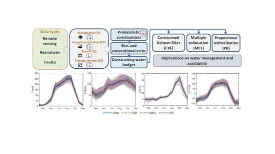
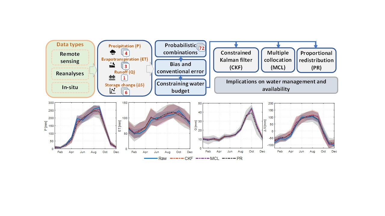
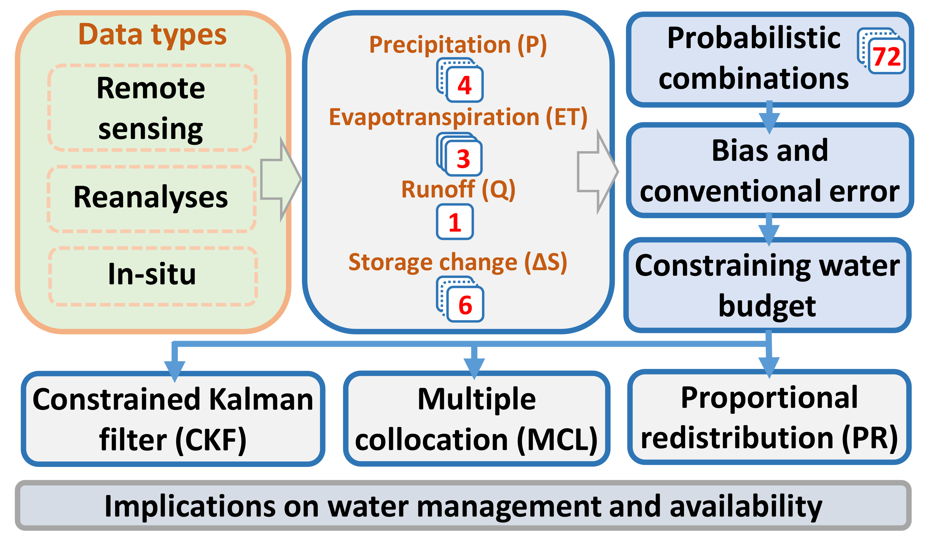
2.3. Enforcing Water Budget Closure

We apply three available closure techniques, namely Constrained Kalman Filter (CKF) [1], Multiple Collocation (MCL) [24], and Proportional Redistribution (PR) [2], to enforce water budget closure in upper CPRB. Since the true value of any variable (P, ET, and ∆S) is unknown, the ensemble means across all datasets for respective variables are assumed to represent true values [7]. For Q, since the gage type and stage-discharge relationship were not available, runoff volume and associated uncertainties are assumed to be inversely proportional, as reported in an observational study [25]. We used a time series of uncertainty linearly varying from 2.3% to 28.8%, corresponding from highest to the lowest flow (Q).

2.3.1. Constrained Kalman Filter (CKF)

Assuming that errors in all water budget components follow zero-mean Gaussian distributions and are non-correlated among various estimates, the error covariance for an estimate can be represented as,

$${\mathsf{\epsilon }}_{\mathrm{xx}}=\overline{\left({\mathrm{x}}^{\prime }-{\mathrm{x}}_{\mathrm{t}}\right){\left({\mathrm{x}}^{\prime }-{\mathrm{x}}_{\mathrm{t}}\right)}^{\mathrm{T}}}$$

(4)

where ${\mathrm{x}}^{\prime }$ and ${\mathrm{x}}_{\mathrm{t}}$ are the state estimates, and its true values, respectively. Water budget closure constraints (i.e., $\mathsf{\epsilon }$) that assume non-correlated errors [5] take the form,

$${\mathsf{\epsilon }}_{\mathrm{xx}}=\left[\begin{array}{cccc}{\mathsf{\epsilon }}_{\mathrm{P}-\mathrm{P}}& {\mathsf{\epsilon }}_{\mathrm{P}-\mathrm{ET}}& {\mathsf{\epsilon }}_{\mathrm{P}-\mathrm{Q}}& {\mathsf{\epsilon }}_{\mathrm{P}-\Delta \mathrm{S}}\\ {\mathsf{\epsilon }}_{\mathrm{ET}-\mathrm{P}}& {\mathsf{\epsilon }}_{\mathrm{ET}-\mathrm{ET}}& {\mathsf{\epsilon }}_{\mathrm{ET}-\mathrm{Q}}& {\mathsf{\epsilon }}_{\mathrm{ET}-\Delta \mathrm{S}}\\ {\mathsf{\epsilon }}_{\mathrm{Q}-\mathrm{P}}& {\mathsf{\epsilon }}_{\mathrm{Q}-\mathrm{ET}}& {\mathsf{\epsilon }}_{\mathrm{Q}-\mathrm{Q}}& {\mathsf{\epsilon }}_{\mathrm{Q}-\Delta \mathrm{S}}\\ {\mathsf{\epsilon }}_{\Delta \mathrm{S}-\mathrm{P}}& {\mathsf{\epsilon }}_{\Delta \mathrm{S}-\mathrm{ET}}& {\mathsf{\epsilon }}_{\Delta \mathrm{S}-\mathrm{Q}}& {\mathsf{\epsilon }}_{\Delta \mathrm{S}-\Delta \mathrm{S}}\end{array}\right]=\left[\begin{array}{cccc}{\mathsf{\epsilon }}_{\mathrm{P}-\mathrm{P}}& 0& 0& 0\\ 0& {\mathsf{\epsilon }}_{\mathrm{ET}-\mathrm{ET}}& 0& 0\\ 0& 0& {\mathsf{\epsilon }}_{\mathrm{Q}-\mathrm{Q}}& 0\\ 0& 0& 0& {\mathsf{\epsilon }}_{\Delta \mathrm{S}-\Delta \mathrm{S}}\end{array}\right]$$

(5)

Equation (5) was further solved for ${\mathsf{\epsilon }}_{\mathrm{xx}}$ and Kalman gain in accordance with Pan and Wood [26] and Pan et al. [1].

2.3.2. Multiple Collocation (MCL)

Assuming all the N (=4,3,1, and 6 for P, ET, Q, and ∆S, respectively) sets of estimates (with n monthly values in each estimate; n = 216 in our study) of a variable are unbiased, the distance between any two estimates (${\mathrm{x}}_{\mathrm{i}}$ and ${\mathrm{x}}_{\mathrm{j}}$), measured as root mean squared (RMS) distance can be written as,

$${\mathrm{d}}_{\mathrm{ij}}=\sqrt{\frac{1}{\mathrm{n}}{\displaystyle \sum }_{\mathrm{k}=1}^{\mathrm{n}}{\left({\mathrm{x}}_{\mathrm{i},\mathrm{k}}-{\mathrm{x}}_{\mathrm{j},\mathrm{k}}\right)}^2}; \forall \mathrm{i}=1:\mathrm{N}$$

(6)

Considering the errors of all estimates are uncorrelated (i.e., two errors are orthogonal), the Pythagorean Theorem in Hilbert space becomes,

$${\mathrm{d}}_{\mathrm{it}}^2+{ \mathrm{d}}_{\mathrm{jt}}^2={ \mathrm{d}}_{\mathrm{ij}}^2 ; \forall \mathrm{i}\ne \mathrm{j}$$

(7)

where, subscript t denotes the true value of a water budget component which, in the current study, is assumed equal to the ensemble mean for P, ET, ∆S. The Pythagorean constraints for any system (e.g., N = 3) can be written by Equation (8) in vector form [24],

$$\left[\begin{array}{ccc}1& 1& 0\\ 1& 0& 1\\ 0& 1& 1\end{array}\right]\left[\begin{array}{c}{\mathrm{d}}_{1\mathrm{t}}^2\\ {\mathrm{d}}_{2\mathrm{t}}^2\\ {\mathrm{d}}_{3\mathrm{t}}^2\end{array}\right]=\left[\begin{array}{c}{\mathrm{d}}_{12}^2\\ {\mathrm{d}}_{13}^2\\ {\mathrm{d}}_{23}^2\end{array}\right]$$

(8)

where, for example, ${\mathrm{d}}_{23}^2$ is the mean squared distance between estimates 2 and 3. Moreover, since there is no exact solution for over-constrained (N > 3; ∆S in the current study) systems, MCL uses a least-squares solution to minimize Pythagorean distances of the constraints to reach the best ‘compromise’ [24]. Water budget closure error is then redistributed to the various components proportional to their relative distance (not the magnitude like in PR; explained below) from the true value (ensemble mean).

2.3.3. Proportional Redistribution (PR)

PR is the simplest method assuming that the relative errors for any given water budget component at a given time step are proportional to its relative magnitude [2],

$${\mathrm{x}}_{\mathrm{i}}^{\prime }={\mathrm{x}}_{\mathrm{i}}-\mathrm{r}\left(\mathrm{G}\right)\left(\frac{\left|{\mathrm{x}}_{\mathrm{i}}\right|}{{{\displaystyle \sum }}_{\mathrm{j}=1}^4{\mathrm{x}}_{\mathrm{j}}}\right)$$

(9)

where $\mathrm{i}$ corresponds to the $\mathrm{i}$th element, and other parameters have values as explained earlier.

2.4. Data Used

Datasets of water budget components are from reanalysis, remote sensing, and observed in-situ records, spanning May 2002 to April 2020 (

Table 1. Summary of precipitation and evapotranspiration datasets spanning May 2002 to April 2020 (except for TRMM data which is for May 2002 to December 2019). (for acronyms and abbreviations, please refer to the Appendix A).

Variable	Dataset	Spatial Resolution and Frequency	References	Remarks
Precipitation	TRMM (TMPA) 3B42 V7	0.25° × 0.25° Daily	TRMM [39]	Derived by the multi-channel microwave and IR observations from satellites, followed by rescaling based on gauge observations, summing (and applying a factor of three) 3-hourly valid retrievals in a grid cell.
	GPM IMERG	0.1° × 0.1° Monthly	Huffman et al. [40]	Intercalibrates and merges the satellite microwave precipitation estimates with microwave-calibrated IR satellite estimates and gauge data using the quasi-Lagrangian time interpolation.
	CHIRPS-2.0	0.05° × 0.05° Daily	Funk et al. [41]	Incorporates satellite data from NASA and NOAA, and in-situ station data followed by the removal of systematic bias based on IR CCD observations.
	GPCP Version 2.3	2.5° × 2.5° Monthly	Adler et al. [42]	Integration of various rain gauge stations, satellite data sets and sounding observations.
	PERSIANN-CDR	0.25° × 0.25° Daily	Hsu et al. [43]	Uses the ANN algorithms on GridSat-B1 IR satellite data, ANN training using the NCEP stage IV precipitation data (hourly), and finally bias adjusted using the GPCP monthly product version 2.2.
Evapotranspiration	GLDAS NOAH v2.1	0.25° × 0.25° Monthly	Beaudoing et al. [44]	Temporal averaging of 3-hourly GLDAS-2.1 Noah output (Princeton meteorological forcing input data) to produce monthly data followed by the post-processing with the MOD44W MODIS land mask.
	GLEAM v3.5a	0.25° × 0.25° Daily	Martens et al. [45]	Uses PT equation with an updated water balance module and updated evaporative stress functions. Extracts maximum information from different components of terrestrial ET (evaporation from bare land and open water, interception, sublimation, transpiration) from the satellite databases.
	MERRA-2	0.5° × 0.625° Daily	Reichle et al. [46]	Jointly uses the atmospheric general circulation model, atmospheric assimilation system (including modern hyperspectral radiance and microwave observations), an interactive aerosol scheme, and the observed precipitation at the land surface.

and

Table 2. Summary of terrestrial water storage (TWS) datasets used in this study from May 2002 to April 2020.

Variable	Dataset	Spatial Resolution and Frequency	References	Remarks
Terrestrial water storage	CSR Mascons RL06M v02	0.25° × 0.25° Monthly	Save et al. [47], Save [48]	Corrected for representation on ellipsoidal Earth applied separately to land and ocean to minimize signal leakage. ∆C30 coefficient was replaced with a more accurate estimate from SLR for computing GRACE-FO mascons.
	JPL Mascons RL06M v02	0.5° × 0.5° Monthly	Wiese et al. [49], Watkins et al. [50]	Coastline Resolution Improvement (CRI) filter applied, which leads to reduced leakage errors across coastlines. Realistic geophysical information is introduced during the solution inversion to intrinsically remove correlated error
	GFZ Spherical Harmonics RL06 Level-2	1° × 1° Monthly	Dahle et al. [51], Dahle et al. [52]	A number of modifications in the static gravity background field, time-variable gravity background field, atmospheric mass variability models, model for planetary ephemerides, parameterization of the accelerometers, processing of GPS constellation have been incorporated compared to the previous versions.
	COST G Spherical Harmonics RL02	1° × 1° Monthly	Meyer et al. [53], Jean et al. [54]	A harmonization and quality control of the individual input solution level is performed, followed by application of variance component estimation. The resulting COST-G combined gravity fields are validated by assessing their signal and noise content in the spectral and spatial domain.
	CNES GRGS Spherical Harmonics RL05	1° × 1° Monthly	Lemoine et al. [55]	Latest version of L1B measurements, new model of ocean tides (FES2014b), and IGS orbits and clocks are used instead of GRGS ones are used. The normal matrices are first diagonalized, ordered by decreasing order of the Eigenvalues, and only the best-defined sets of linear combinations of the SH are solved, unlike other SH solutions, which use simple Cholesky inversion.
	GSFC Mascons RL06v1.0	0.5° × 0.5° Monthly	Loomis et al. [56]	GSFC monthly regularization matrices are determined by analyzing the geographical binning of the inter-satellite range-acceleration pre-fit residuals. The 1-arc-degree equal-area values have been placed on an equal angle 0.5° × 0.5° grid. Land values are determined with a least-squares estimator that conserves mass over each region.

). All water budget components used in this analysis are basin averaged monthly time series represented as equivalent water depth (mm). Data products showing favorably similar inter-annual and seasonal dynamics are used for calculating the coefficient of variation (CV = standard deviation/ensemble mean).

2.4.1. Precipitation and Evapotranspiration

Precipitation (rainfall + snowfall) and evapotranspiration (evaporation + transpiration) are the largest incoming and outgoing water fluxes in any hydrologic system, respectively, and play significant roles in the distribution and availability of water resources in a region [27]. Traditional in-situ point-based monitoring of both P and ET is costly, restricted to local scales, and prone to large uncertainties, especially in the data-limited regions like the upper CPRB (with a meager rain gauge density of 0.5 rain gauges per 1000 km²). Therefore, to get the spatially distributed continuous time series, we have retrieved data from multiple sources. A detailed list of various gridded datasets used for precipitation and evapotranspiration, their sources, and spatiotemporal resolutions are shown in Table 1.

2.4.2. Terrestrial Water Storage

Various datasets for terrestrial water storage (TWS) and their salient features are listed in Table 2. Spherical harmonics (SH) coefficients, used in TWSA products, are processed for noise reduction at high frequencies (low wavelength) using low-pass filtering (e.g., 300  km Gaussian filtering, truncation at the maximum order and degree 60, de-striping), which would have inevitably led to signal errors [28,29,30]. These errors consist of bias (leakage-out; signal loss within specific study area due to the basin function/filtered averaging kernel) and leakage (leakage-in; contamination/gain in the target signal from the surrounding region) errors [28,31]. To restore true signals, a number of model-dependent (additive [32], scaling [33], and multiplicative [31]; all of which primarily use outputs from the hydrological models) or model-independent (i.e., data-driven [34]) approaches have been employed in globally distributed river basins. Since the data-driven approach outperforms other methods in the upper CPRB, we employ the same for restoring GRACE signals. Overall, an inter-comparison of filtered GRACE TWSA and $\Delta \mathrm{S}$ shows strong agreement between all products. The variance (scatter RMS varying from 12.5 to 19.5 mm) among different GRACE products range within error bounds of the GRACE data with no significant biases, which is consistent with previous studies [2,30]. Since there is minimal signal loss attributed to the regularization and post-fit residual analysis, no signal restoration procedures are required for GRACE Mascon (mass concentration) solutions [35]. We assume no bias between GRACE and GRACE-FO data following recent studies that reported negligible intermission biases over the Central United States, Middle East, Europe, Australia [36], and ice caps and glaciers [37,38].

2.5. Artificial Neural Network

GRACE, operational from April 2002 to June 2017, and GRACE-FO, operational from June 2018 onwards, monitor Earth’s gravity at an unprecedented spatiotemporal resolution [57]. GRACE products have been revolutionary in understanding terrestrial water storage dynamics, sea-level change, melting of polar ice, and climate change [10,58]. GRACE products have frequent gaps, especially post 2011, and an 11-month gap between GRACE and GRACE-FO datasets (see footnote of

Table 3. Performance indicators (r, NRMSE, and NSE) for all six TWSA products during training and validation phases.

TWSA Product	Training (161 Values; May 2002–June 2017) *			Validation (21 Values; June 2018–April 2020) **
	r	NRMSE	NSE	r	NRMSE	NSE
CSR	0.97	0.27	0.93	0.97	0.32	0.92
JPL	0.97	0.24	0.94	0.96	0.26	0.93
GFZ	0.94	0.32	0.89	0.91	0.37	0.82
COST-G	0.96	0.28	0.92	0.95	0.35	0.90
CNES GRGS	0.96	0.29	0.91	0.97	0.28	0.92
GSFC	0.95	0.30	0.90	0.96	0.28	0.90

* 21 values (June 2002, July 2002, June 2003, January 2011, June 2011, May 2012, October 2012, March 2013, August 2013, September 2013, February 2014, July 2014, December 2014, May 2015, June 2015, October 2015, November 2015, April 2016, September 2016, October 2016, February 2017) were missing during April 2002–June 2017. ** 2 values (August 2018, September 2018) were missing during June 2018–April 2020.

for detailed information of data gaps). We developed a multilayer perceptron artificial neural network (ANN) model for filling data gaps in and between GRACE and GRACE-FO TWSA time series. The ANN, a nonparametric modeling technique, seeks to learn the functional mapping ($\mathrm{f}$) between a set of predictors or states ($\mathrm{x}$) and the target or output variable ($\mathrm{y}$), when there is a lack of conventional physics-based models. Mathematically, ANN can be represented as below [4,59]

$$\mathrm{y}=\mathrm{f}\left(\mathrm{x}\right)+\mathsf{\epsilon }$$

(10)

where $\mathsf{\epsilon }$ is the process noise. The ANN model consists of three components: an input layer (predictors), a hidden layer, and an output layer. A combination of monthly time series of various hydroclimatic (temperature, precipitation, evapotranspiration) and water storage components (soil moisture storage, surface runoff, TWS from GLDAS) were tested as predictors during model calibration, and the best performing set was further used for model validation and prediction. The hidden layer of the ANN is comprised of hidden neurons whose numbers were optimized with the coupled genetic algorithm and finalized as six, corresponding to the minimum root mean square error and the maximum Nash-Sutcliffe efficiency during model calibration. Each neuron in the hidden layer is the weighted sum of the predictors,

$${\mathrm{a}}_{\mathrm{k}}={\displaystyle \sum }_{\mathrm{i}=1}^{\mathrm{P}}{\mathrm{w}}_{\mathrm{ki}}{\mathrm{x}}_{\mathrm{i}}+{\mathrm{w}}_{\mathrm{ki}}$$

(11)

where, ${\mathrm{a}}_{\mathrm{k}}$ is hidden neuron (k = 1, 2,…5), ${\mathrm{w}}_{\mathrm{ki}}$ is the weight associated with the input layer $\mathrm{i}$ ($=1,2,\dots \mathrm{P}$) and neuron $\mathrm{k}$, and ${\mathrm{w}}_{\mathrm{ki}}$ is the bias term. The weighted sum is then utilized to calculate the output variable (i.e., TWSA) via a transfer function as below,

$${\mathrm{z}}_{\mathrm{k}}=\mathsf{\Psi }\left({\mathrm{a}}_{\mathrm{k}}\right)$$

(12)

where, ${\mathrm{z}}_{\mathrm{k}}$ is the output, and $\mathsf{\Psi }$ is the transfer function. Building upon a previous study [4], we utilized the ANN model for gap-filling between GRACE and GRACE-FO and other data gaps due to battery management. TWSA time series from May 2002 to June 2017 (GRACE) and June 2018 to April 2020 (GRACE-FO) were used for calibration and validation, respectively. Model performance during both calibration and validation phases is assessed using various statistical parameters, including the Pearson correlation coefficient (r), normalized root mean square error (NRMSE), and Nash-Sutcliffe efficiency (NSE).

3. Results and Discussion

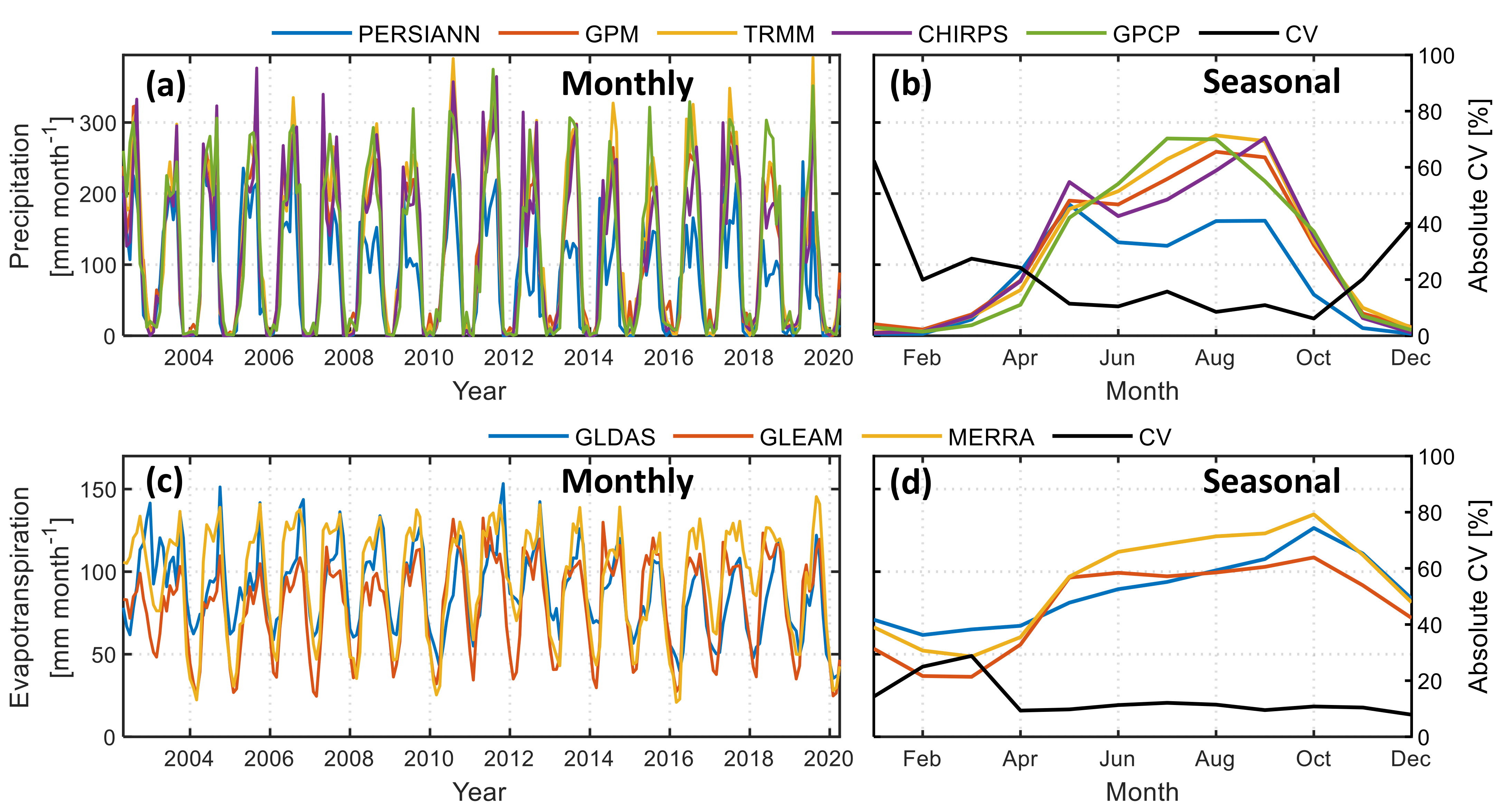
3.1. Variability among Precipitation and Evapotranspiration Data Products

Precipitation: Although all precipitation products have similar dynamics in both monthly and seasonal time series (Figure 3a,b) and are highly correlated (r $\ge$ 0.9 except for PERSIANN-CDR), there are substantial deviations in magnitude (as high as 150 mm in July). Despite the adjustments with GPCP data [60], PERSIANN-CDR, in general, underestimates (average ~110 mm per month, equivalent to ~35%, during the rainy season) precipitation relative to the ensemble mean; meanwhile, other products fluctuate between overestimation or underestimation. PERSIANN-CDR tends to underestimate heavy precipitation (≥20 mm d⁻¹) events and therefore results in the dampened monthly and seasonal cycles, and hence was excluded from further analysis. Deviations among data products, even within the same category (satellite-related, reanalysis, gauge-based), depends on a multitude of factors such as location, topography, climate (e.g., arid and semi-arid regions possess higher discrepancies among various products than in humid regions; [61]), physical inadequacies (e.g., including few cloud-related parameters, or few gauge observations) of various retrieval algorithms (e.g., in PERSIANN-CDR case), interpolation processes, and bias adjustments [62]. Incorporation of few but overlapping gauge data in sparsely gauged basins, like the upper CPRB, can also result in a smaller spread among various precipitation products, possibly due to limited uncertainties in gridding and undercatch correction procedures [1]. Consistent with the tropical climate regime, GPM, TRMM, CHIRPS, and GPCP show precipitation patterns with reasonably consistent distributions (maximum seasonal variation of 86 mm in July) and hence were considered for further analysis (Figure 3). The average rainy season CV is 10.5% (maximum of 15.7% in July) and non-rainy season CV is 32.4% (May to October); the latter is due to the near-zero precipitation values from all four products. The first precipitation peak in May is from the onset of the western monsoon season (May–October) and tropical rainfalls from the South China Sea. The second peak in August–September (variable among products) corresponds with monsoon rainfall and tropical storms in the basin, and the dry season rainfall is attributable to southern winds and the northeastern monsoon (Figure 1).

Evapotranspiration: ET products reveal complex monthly and seasonal time series over the basin due to high spatiotemporal variability in soil moisture, meteorological conditions, and other phenological factors [7,63]. Despite similar dynamics in annual and seasonal cycles, the three ET products possess a widespread (i.e., less agreement) relative to the precipitation products (Figure 3), which is consistent with previous water budget assessments [1,2,8]. Seasonal dynamics of all three ET products have more stable behavior than P (Figure 3c,d), attributable to the humid climate and intense irrigation (by surface water and groundwater in both wet and dry seasons), which reduces ET’s dependence on soil moister availability [64]. GLEAM underestimates ET, whereas GLDAS provides overestimates, especially during the dry period. Underestimation by GLEAM is likely attributable to inadequate representation of the evaporation from water bodies in the region and underestimation of canopy interception, vegetation optical depth, and the water extent in the rainforests. Overestimation by MERRA in the tropical CPRB is consistent with the Zhang et al. [7] Climate Data Record (CDR). Average dry and wet seasonal ET variations are comparable with the CV of 13.4% and 10.8%, respectively.

3.2. Observed Runoff

The mean monthly runoff recorded at the Nakhon Sawan C2 station ranges from 3.05 mm (February 2020) to 115.67 mm (October 2006), while the seasonal time series record maximum and minimum values in October (44.48 mm) and April (8.05 mm), respectively (Figure 4). The high correlation of the seasonal runoff cycle with one and two months (r~0.92 for both) lag with precipitation is attributable to the memory of natural hydrological processes (e.g., baseflow) in the basin. The basin experienced the most severe flood within the past five decades in 2011, where runoff records show the second largest peak of 109.45 mm in October 2011, followed by 74.17 mm and 66.08 mm in October 2002 and October 2017, respectively. Note, all of which correspond with flood events. Minimal monthly runoff of 3 to 5 mm was observed during the dry season of drought years 2004–2005, 2010, 2013, 2015–2016, and 2020 (Figure 4).

3.3. Generating Continuous TWSA Time Series

Since all six TWSA time series from various data processing centers utilize common GRACE and GRACE-FO data, they agree favorably in terms of amplitude and dynamics for both the monthly and seasonal time series (Figure 5a,b). The ANN model performed reasonably well (r $\ge$ 0.95, NRMSE $=$ 0.24 − 0.37, and NSE $\ge$ 0.89) for all six TWSA time series during both calibration and validation phases (Table 1, Figure A1) which can be ascribed to (a) small uncertainties in GRACE data, primarily from the short-wavelength signals and subsequent filtering processes which tends to be smaller for large areas, (b) ample predictor availability from ancillary data sources, and (c) the embedded genetic algorithm avoids underfitting or overfitting in the ANN model. An example for the modeled and observed time series is shown in Figure A1 to highlight the ANN model’s performance during calibration and validation phases. The current ANN model is used for data gap filling between GRACE and GRACE-FO TWSA time series (11 values) and for filling intermittent data gaps (23 values) occurring approximately every six months starting from 2011; the latter of which has been filled by linear interpolation of the two or more bounding values in previous studies. This linear interpolation may induce uncertainties by (a) underestimating the actual (positive/negative peak) TWS if the data gap happens to be in the peak of the wet or dry season, or (b) overestimation or underestimation in case of the high short-term fluctuations in the TWS. Furthermore, these instances of overestimation or underestimation might lead to inappropriate inferences in the river basins like CPRB, which is highly vulnerable to floods and droughts. Therefore, we have attempted to quantify various water budget components as accurately as possible.

A number of floods (e.g., 2011) and droughts (e.g., 2015, 2016) experienced in the basin are evident in the TWSA time series [4]. Subsequently derived $\Delta \mathrm{S}$ agrees well with a minimal scatter of <20% (Figure 5c,d). Some minor discrepancies among TWSA products can be attributed to different processing algorithms and correction and filtering methods used by various data centers. However, all variations are well within the error ranges of the GRACE data with no significant biases, which is consistent with the previous studies [2,30].

3.4. Raw Ensembles of the Water Budget and Residual Error

Seasonal variations of water budget components (shown in Figure 6)—excluding estimates from model products (e.g., GLDAS) which neglect anthropogenic activities—possess embedded effects of both natural and human-induced climate variability (e.g., reservoirs management, groundwater abstraction, irrigation, etc.) and has strong seasonality. Generally, P controls the other water cycle components during the rainy season (May to October) since the anthropogenic activities are minimal during this period, with an opposite situation in the dry season (November to April) (Figure 6). P attains a minimum of ~7–10 mm (December–February) and a maximum of 267.73 mm (September). ET has a minimum of ~50 mm (February–March) and continually increases from May to October from the onset of the monsoon season with a maximum of 123.24 mm (October). $\Delta \mathrm{S}$ is primarily driven by the net precipitation (P-ET) and shows a minimum of −105 mm in December and a maximum of 103 mm during June to August. Maxima and minima of all the water budget components have the lag behavior varying between one to three months from each other.

The mean monthly residual error averaged across all combinations of water budgets is 14.37 mm month⁻¹ for the basin and is consistent with the previously reported tendency for positive residuals in lower latitude basins [2]. The mean monthly error accounts for about 15% (consistent with Rodell et al. [5]) and 16% of the ensemble mean of monthly P and ET, respectively. An increasing trend of 0.03 mm month⁻¹ in residual errors may partly be attributed to increased human interventions. Specifically, the CPRB has hosted a 10% increase in the area equipped for irrigation from 5830 × 10³ ha to 6415 × 10³ ha from 2002 to 2020 in Thailand; [65], which is expected to drive increasingly negative biases in model-based ET due to missing irrigation information. Although overall variations of the residual error in the basin are minimal (mean of the % variation = −0.02%), the residual error is more frequently positive than negative and generally possesses relatively high fluctuations from April to November (Figure 6). The tendency of the residual error to be positive can be mainly explained by either wet biases in precipitation or by dry biases in the ET and $\Delta \mathrm{S}$ (or a combination of these factors).

Since ground-truthing for most of the water budget variables is unavailable in data-limited/data-scarce river basins such as the upper CPRB, a set of data products having large errors in different directions (e.g., underestimated P, overestimated ET, Q, and $\Delta \mathrm{S}$ in case of positive residuals) may erroneously lead to minimal or even near-zero residuals in the water balance resulting in misleading interpretation and implications. Therefore, three water balance closure techniques of varying mathematical complexity are applied to attain the physical water balance constraint for each unique realization of the water budget. Since an independent and uncorrelated a priori bias in various datasets cannot be known, we assume corrected values as ‘true’; note that the development of more robust and advanced techniques may lead to more realistic results.

3.5. Comparison of Three Water Budget Closure Techniques

All three closure techniques perform similarly across water balance components without presenting unidirectional characteristics (Figure 7). The proportional redistribution (PR) method generally provides the lowest and highest closure constraints (Equation (9)) for P, ET, and Q in case of wet and dry biases, respectively (Figure 7). $\Delta \mathrm{S}$ closure constraints are persistently positive during the dry season. P closure constraints are typically negative (indicating a wet bias in P), while those for ET, Q and $\Delta \mathrm{S}$ have opposite signs during respective time periods. Although closure constraints are minimal during October-November in P, other components (Q, ET, and $\Delta \mathrm{S}$) have dry biases attributed to the negative residual during these months. Since Q is observed in-situ, it generally possesses low constraint values except for the month of October (corresponding to the highest Q), particularly from the PR approach.

Despite the mixed behavior of closure constraints in seasonal time series, the mean annual variability of various components reveals wet biases in P and Q and dry biases in ET and $\Delta \mathrm{S}$ (Figure 8 and Figure A2). The absolute magnitude of these biases follows the order of variability as $\Delta \mathrm{S}$> P > ET > Q. One notable inference is that negative (or positive) closure constraints for P do not necessarily imply positive (or negative) constraints in the remaining components on annual scales. All components may have similar constraints (same sign/direction: positive or negative) but with different magnitudes, as revealed in the annual time series (e.g., the year 2012; Figure 8). Wet bias (overestimation) of P or dry bias (underestimation) of ET, especially in the rainy season, may lead to misinterpretation of regional flood and drought potential and projections. Similarly, accurate assessments of Q and $\Delta \mathrm{S}$ may inform dam reservoir operations (water release amount and timing) and agricultural water management (e.g., partitioning and dependence on surface water and groundwater extraction).

3.6. Long-Term Variations and Trends in Corrected Water Budget Components

We calculate long-term annual means of various water storage components (P, ET, Q) from 2003 to 2019 and compared them with a previous study [66] focusing on global estimates for the same period and other global studies. Long term means of P, ET, and Q for the upper CPRB are 1355 mm yr⁻¹ (global mean 811 mm yr⁻¹, [66]), 1086 mm yr⁻¹ (1.8 to 3.3 times larger than global estimates based on various methods [5,66]), and 210 mm yr⁻¹ (global mean of 366 mm yr⁻¹ [66]), respectively. Uncertainties of all the water budget components are decreased after applying closure constraints (shaded areas in Figure 8). Corresponding uncertainties for corrected P (${\mathsf{\sigma }}_{\mathrm{P}}$), Q (${\mathsf{\sigma }}_{\mathrm{Q}}$), ET (${\mathsf{\sigma }}_{\mathrm{ET}}$), and $\Delta \mathrm{S}$ (${\mathsf{\sigma }}_{\Delta \mathrm{S}}$), calculated as the standard deviation across data products, are 10.4, 4.7, 9.12, and 2.6 mm month⁻¹, respectively. Intercomparison of the annual trends in raw and corrected components reveal that P has the highest change (raw vs corrected trends: −1.85 to −4.67 mm yr⁻¹) followed by ET (−1.94 to −1.09 mm yr⁻¹) and Q (−4.38 to −4.25 mm yr⁻¹). Corrected long-term linear trends reveal a 1.0% decrease in P, 8.6% increase in ET, and 13% decrease in Q (+3%, +10%, and −6% change in P, ET, Q, respectively, globally [66]). ET/Q has an increasingly significant trend, which suggests that P is increasingly partitioned in ET rather than Q (i.e., decreasing runoff efficiency). Increases in ET can be associated with the joint impact of ENSO events with increasing temperature and irrigation in the region [4]. This result agrees with the premise of intensification of the water cycle in a warming climate [66]. Although the majority of deforestation in CPRB occurred in the late 20th century (especially in the 1970s and 1980s), ongoing dynamic and heterogeneous land use land cover changes in the basin may partially influence ET trends. The observed increase in ET/Q indicates a potential overreliance on groundwater in the future if the current trend persists. Further human influences of irrigation and reservoir management may be implicated in our water budget closure assessment. For example, corrected ET is larger than raw ET. This computed underestimate is consistent with expected biases from ET products that do not fully account for irrigation.

Additionally, the long-term average of $\Delta \mathrm{S}$ is persistently positive, even in some drought years (e.g., 2015) (Figure 8). This may be partially attributable to dam reservoir operations in the region that maintains water in CPRB or to the relative redistribution of biases among other water budget variables (P, ET, and Q); the latter of which can simply be a mathematical artifact and should be investigated further. These observationally-based signals of human interventions with the water cycle are important to consider for risk mitigation associated with extreme hydrologic events and agricultural water management in the basin. We acknowledge uncertainties and limitations associated with retrieval algorithms, models’ physical structures, systematic biases, and limited data records implicit in data products used herein. Thus, future water budget assessments over CPRB can benefit from the use of higher spatial and temporal resolution data with longer records followed by downscaling/reconstruction (e.g., [67]). Continuously increasing density of rain gauges, ET flux towers, and groundwater monitoring will further assist in understanding the complex interactions of human-induced changes and climate variability on regional hydrology.

4. Conclusions

In this study, we have quantified relative biases in water budget components to better understand regional earth system processes and water dynamics in the upper Chao Phraya River Basin from May 2002 to April 2020. The basin is highly vulnerable to hydroclimatic extremes, plays a key role in the policymaking in Thailand and subsequently in neighboring countries, and possesses a complex existing water governance framework with a multitude of institutions (as many as 31 ministerial departments, among other national and autonomous agencies; [12,68]). The major findings of our study are summarized below,

• Various data products, which are based on remote sensing, reanalysis, and in-situ observations, have similar seasonal and annual dynamics, and the variations across products can be attributed to the different retrieval algorithms, model inadequacies, and other biases.
• The ANN model has the potential to fill data gaps between the GRACE and GRACE-FO TWS time series (11 months missing values) and for the sporadically missing values due to battery management practices (a total of 23 missing values during the study period); the latter of which is otherwise filled by using the linear interpolation of the bounding values and thus may underestimate the TWS especially during the peak of the dry or wet season.
• Generally, P tends to have wet bias while ET, Q, and $\Delta \mathrm{S}$ have dry biases. Seasonal time series of the closure constraints of various water budget components reveal a mixed behavior, while the absolute mean annual variability follows the order as $\Delta \mathrm{S}$> P > ET > Q. Interestingly, a negative (or positive) closure constraint in P does not necessarily imply a positive (or negative) constraint in the remaining components on an annual scale. Knowledge of wet or dry biases of individual components of the water cycle has potential implications for water resources, climate, and agriculture in the basin. For example, correction of an overestimation (underestimation) implicit to P (ET) in the rainy season may avert inaccurate flood (drought) projections.
• The magnitude and sign of closure constraints on various water budget components using the three closure techniques and the resultant partitioning of the water cycle when combined with long term trends in various hydrological and water storage components in our companion study [4] can be effectively used to inform water management especially for mitigation of the adverse effects of drought and floods and for water availability in the basin.
• Although the currently employed water balance closure techniques utilize the unique information from the available scatter of various data products for any given component, the derived combination, though physically consistent, may not be most accurate. This could happen because of similar biases (e.g., dry bias in both P and ET), biases with opposite directions, correlation among various components arising from geophysical variabilities, or simply due to the mathematical artifact [69]. However, the results may serve as the basis for the starting point of getting insights into water availability and other hydrological applications for guiding potential users.

Our assessment provides insights into relative uncertainties of observed and modeled water budget components for the study period and may be utilized for enabling efficient water management and related policymaking. Results may be useful for further segregating the impacts of natural and anthropogenic factors on hindcasted or forecasted water budget components and subsequent potential adaptation measures. The improved understanding of regional water cycle dynamics is of utmost importance and has potential in benchmarking regional hydroclimate models for better understanding, quantification, and predicting the distribution and variability of the terrestrial water cycle and ultimately leading to reduced water budget imbalance.

References

1. Pan, M.; Sahoo, A.K.; Troy, T.J.; Vinukollu, R.K.; Sheffield, J.; Wood, A.E.F. Multisource estimation of long-term terrestrial water budget for major global river basins. J. Clim. 2012, 25, 3191–3206. [Google Scholar] [CrossRef]
2. Abolafia-Rosenzweig, R.; Pan, M.; Zeng, J.L.; Livneh, B. Remotely sensed ensembles of the terrestrial water budget over major global river basins: An assessment of three closure techniques. Remote Sens. Environ. 2021, 252, 112191. [Google Scholar] [CrossRef]
3. Abhishek; Kinouchi, T. Synergetic application of GRACE gravity data, global hydrological model, and in-situ observations to quantify water storage dynamics over Peninsular India during 2002–2017. J. Hydrol. 2021, 596, 126069. [Google Scholar] [CrossRef]
4. Abhishek; Kinouchi, T.; Sayama, T. A comprehensive assessment of water storage dynamics and hydroclimatic extremes in the Chao Phraya River Basin during 2002–2020. J. Hydrol. 2021, 603, 126868. [Google Scholar] [CrossRef]
5. Rodell, M.; Beaudoing, H.K.; L’Ecuyer, T.S.; Olson, W.S.; Famiglietti, J.S.; Houser, P.R.; Adler, R.; Bosilovich, M.G.; Clayson, C.A.; Chambers, D.; et al. The observed state of the water cycle in the early twenty-first century. J. Clim. 2015, 28, 8289–8318. [Google Scholar] [CrossRef]
6. Rosenzweig, C.; Karoly, D.; Vicarelli, M.; Neofotis, P.; Wu, Q.; Casassa, G.; Menzel, A.; Root, T.L.; Estrella, N.; Seguin, B.; et al. Attributing physical and biological impacts to anthropogenic climate change. Nature 2008, 453, 353–357. [Google Scholar] [CrossRef]
7. Zhang, Y.; Pan, M.; Sheffield, J.; Siemann, A.L.; Fisher, C.K.; Liang, M.; Beck, H.E.; Wanders, N.; MacCracken, R.F.; Houser, P.R.; et al. A Climate Data Record (CDR) for the global terrestrial water budget: 1984-2010. Hydrol. Earth Syst. Sci. 2018, 22, 241–263. [Google Scholar] [CrossRef] [Green Version]
8. Penatti, N.C.; Almeida, T.I.R.; Ferreira, L.G.; Arantes, A.E.; Coe, M.T. Satellite-based hydrological dynamics of the world’s largest continuous wetland. Remote Sens. Environ. 2015, 170, 31. [Google Scholar] [CrossRef]
9. Sheffield, J.; Ferguson, C.R.; Troy, T.J.; Wood, E.F.; McCabe, M.F. Closing the terrestrial water budget from satellite remote sensing. Geophys. Res. Lett. 2009, 36, 07403. [Google Scholar] [CrossRef]
10. Rodell, M.; Famiglietti, J.S.; Wiese, D.N.; Reager, J.T.; Beaudoing, H.K.; Landerer, F.W.; Lo, M.H. Emerging trends in global freshwater availability. Nature 2018, 557, 651–659. [Google Scholar] [CrossRef]
11. Scanlon, B.R.; Zhang, Z.; Save, H.; Sun, A.Y.; Schmied, H.M.; Van Beek, L.P.H.; Wiese, D.N.; Wada, Y.; Long, D.; Reedy, R.C.; et al. Global models underestimate large decadal declining and rising water storage trends relative to GRACE satellite data. Proc. Natl. Acad. Sci. USA 2018, 115, E1080–E1089. [Google Scholar] [CrossRef] [Green Version]
12. Food and Agriculture Organization of the United Nations (FAO). FAO AQUASTAT Country Profile—Thailand; Food and Agriculture Organization of the United Nations: Rome, Italy, 2011. [Google Scholar]
13. Turral, H.; Burke, J.; Faurès, J.-M. FAO Water Report 36: Climate Change, Water and Food Security; Food and Agriculture Organization of the United Nations: Rome, Italy, 2008; ISBN 9789251067956. [Google Scholar]
14. Supharatid, S. Skill of precipitation projectionin the Chao Phraya river Basinby multi-model ensemble CMIP3-CMIP5. Weather Clim. Extrem. 2015, 12, 14. [Google Scholar] [CrossRef] [Green Version]
15. Sahoo, A.K.; Pan, M.; Troy, T.J.; Vinukollu, R.K.; Sheffield, J.; Wood, E.F. Reconciling the global terrestrial water budget using satellite remote sensing. Remote Sens. Environ. 2011, 115, 1850–1865. [Google Scholar] [CrossRef]
16. Long, D.; Longuevergne, L.; Scanlon, B.R. Uncertainty in evapotranspiration from land surface modeling, remote sensing, and GRACE satellites. Water Resour. Res. 2014, 50, 1131–1151. [Google Scholar] [CrossRef] [Green Version]
17. Gao, H.; Tang, Q.H.; Ferguson, C.R.; Wood, E.F.; Lettenmaier, D.P. Estimating the water budget of major US river basins via remote sensing. Int. J. Remote Sens. 2010, 31, 3955–3978. [Google Scholar] [CrossRef]
18. Wang, S.; Huang, J.; Li, J.; Rivera, A.; McKenney, D.W.; Sheffield, J. Assessment of water budget for sixteen large drainage basins in Canada. J. Hydrol. 2014, 512, 15. [Google Scholar] [CrossRef]
19. Szeto, K.K.; Tran, H.; MacKay, M.D.; Crawford, R.; Stewart, R.E. The MAGS water and energy budget study. J. Hydrometeorol. 2008, 9, 96–115. [Google Scholar] [CrossRef]
20. Panday, P.K.; Coe, M.T.; Macedo, M.N.; Lefebvre, P.; de Almeida Castanho, A.D. Deforestation offsets water balance changes due to climate variability in the Xingu River in eastern Amazonia. J. Hydrol. 2015, 523, 822–829. [Google Scholar] [CrossRef]
21. Armanios, D.E.; Fisher, J.B. Measuring water availability with limited ground data: Assessing the feasibility of an entirely remote-sensing-based hydrologic budget of the Rufiji Basin, Tanzania, using TRMM, GRACE, MODIS, SRB, and AIRS. Hydrol. Process. 2014, 28, 853–867. [Google Scholar] [CrossRef]
22. Azarderakhsh, M.; Rossow, W.B.; Papa, F.; Norouzi, H.; Khanbilvardi, R. Diagnosing water variations within the Amazon basin using satellite data. J. Geophys. Res. Atmos. 2011, 116, 15997. [Google Scholar] [CrossRef] [Green Version]
23. Tang, Q.; Gao, H.; Yeh, P.; Oki, T.; Su, F.; Lettenmaier, D.P. Dynamics of terrestrial water storage change from satellite and surface observations and modeling. J. Hydrometeorol. 2010, 11, 156–170. [Google Scholar] [CrossRef] [Green Version]
24. Pan, M.; Fisher, C.K.; Chaney, N.W.; Zhan, W.; Crow, W.T.; Aires, F.; Entekhabi, D.; Wood, E.F. Triple collocation: Beyond three estimates and separation of structural/non-structural errors. Remote Sens. Environ. 2015, 171, 299–310. [Google Scholar] [CrossRef]
25. Shiklomanov, A.I.; Yakovleva, T.I.; Lammers, R.B.; Karasev, I.P.; Vörösmarty, C.J.; Linder, E. Cold region river discharge uncertainty-estimates from large Russian rivers. J. Hydrol. 2006, 326, 231–256. [Google Scholar] [CrossRef]
26. Pan, M.; Wood, E.F. Data assimilation for estimating the terrestrial water budget using a constrained ensemble Kalman filter. J. Hydrometeorol. 2006, 7, 534–547. [Google Scholar] [CrossRef]
27. Oki, T.; Kanae, S. Global hydrological cycles and world water resources. Science 2006, 313, 1068–1072. [Google Scholar] [CrossRef] [PubMed] [Green Version]
28. Swenson, S.; Wahr, J. Post-processing removal of correlated errors in GRACE data. Geophys. Res. Lett. 2006, 33, 25285. [Google Scholar] [CrossRef]
29. Long, D.; Chen, X.; Scanlon, B.R.; Wada, Y.; Hong, Y.; Singh, V.P.; Chen, Y.; Wang, C.; Han, Z.; Yang, W. Have GRACE satellites overestimated groundwater depletion in the Northwest India Aquifer? Sci. Rep. 2016, 6, 24398. [Google Scholar] [CrossRef]
30. Sakumura, C.; Bettadpur, S.; Bruinsma, S. Ensemble prediction and intercomparison analysis of GRACE time-variable gravity field models. Geophys. Res. Lett. 2014, 41, 1389–1397. [Google Scholar] [CrossRef]
31. Longuevergne, L.; Scanlon, B.R.; Wilson, C.R. GRACE hydrological estimates for small basins: Evaluating processing approaches on the High Plains aquifer, USA. Water Resour. Res. 2010, 46, 46. [Google Scholar] [CrossRef]
32. Klees, R.; Zapreeva, E.A.; Winsemius, H.C.; Savenije, H.H.G. The bias in GRACE estimates of continental water storage variations. Hydrol. Earth Syst. Sci. 2007, 11, 1227–1241. [Google Scholar] [CrossRef] [Green Version]
33. Landerer, F.W.; Swenson, S.C. Accuracy of scaled GRACE terrestrial water storage estimates. Water Resour. Res. 2012, 48, W04531. [Google Scholar] [CrossRef]
34. Vishwakarma, B.D.; Horwath, M.; Devaraju, B.; Groh, A.; Sneeuw, N. A Data-Driven Approach for Repairing the Hydrological Catchment Signal Damage Due to Filtering of GRACE Products. Water Resour. Res. 2017, 53, 9824–9844. [Google Scholar] [CrossRef]
35. Scanlon, B.R.; Zhang, Z.; Reedy, R.C.; Pool, D.R.; Save, H.; Long, D.; Chen, J.; Wolock, D.M.; Conway, B.D.; Winester, D. Hydrologic implications of GRACE satellite data in the Colorado River Basin. Water Resour. Res. 2015, 51, 9891–9903. [Google Scholar] [CrossRef]
36. Landerer, F.W.; Flechtner, F.M.; Save, H.; Webb, F.H.; Bandikova, T.; Bertiger, W.I.; Bettadpur, S.V.; Byun, S.H.; Dahle, C.; Dobslaw, H.; et al. Extending the Global Mass Change Data Record: GRACE Follow-On Instrument and Science Data Performance. Geophys. Res. Lett. 2020, 47, 88306. [Google Scholar] [CrossRef]
37. Velicogna, I.; Mohajerani, Y.; Geruo, A.; Landerer, F.; Mouginot, J.; Noel, B.; Rignot, E.; Sutterley, T.; van den Broeke, M.; van Wessem, M.; et al. Continuity of Ice Sheet Mass Loss in Greenland and Antarctica From the GRACE and GRACE Follow-On Missions. Geophys. Res. Lett. 2020, 47, 87291. [Google Scholar] [CrossRef] [Green Version]
38. Ciracì, E.; Velicogna, I.; Swenson, S. Continuity of the Mass Loss of the World’s Glaciers and Ice Caps From the GRACE and GRACE Follow-On Missions. Geophys. Res. Lett. 2020, 47, 47. [Google Scholar] [CrossRef]
39. Tropical Rainfall Measuring Mission TRMM (TMPA/3B43) Rainfall Estimate L3 1 Month 0.25 Degree × 0.25 Degree V7, Greenbelt, MD, Goddard Earth Sciences Data and Information Services Center (GES DISC). Available online: https://disc.gsfc.nasa.gov/datasets/TRMM_3B42_7/summary (accessed on 15 July 2021).
40. Huffman, G.J.; Stocker, E.F.; Bolvin, D.T.; Nelkin, E.J.; Jackson, T. GPM IMERG Final Precipitation L3 Half Hourly 0.1 degree × 0.1 degree V06, Greenbelt, MD, Goddard Earth Sciences Data and Information Services Center (GES DISC). Available online: https://disc.gsfc.nasa.gov/datasets/GPM_3IMERGM_06/summary?keywords=%22IMERG%20final%22 (accessed on 15 July 2021).
41. Funk, C.; Peterson, P.; Landsfeld, M.; Pedreros, D.; Verdin, J.; Shukla, S.; Husak, G.; Rowland, J.; Harrison, L.; Hoell, A.; et al. The climate hazards infrared precipitation with stations—A new environmental record for monitoring extremes. Sci. Data 2015, 2, 150066. [Google Scholar] [CrossRef] [Green Version]
42. Adler, R.F.; Huffman, G.J.; Chang, A.; Ferraro, R.; Xie, P.P.; Janowiak, J.; Rudolf, B.; Schneider, U.; Curtis, S.; Bolvin, D.; et al. The version-2 global precipitation climatology project (GPCP) monthly precipitation analysis (1979-present). J. Hydrometeorol. 2003, 4, 7541. [Google Scholar] [CrossRef]
43. Hsu, K.L.; Gao, X.; Sorooshian, S.; Gupta, H.V. Precipitation estimation from remotely sensed information using artificial neural networks. J. Appl. Meteorol. 1997, 36, 1176–1190. [Google Scholar] [CrossRef]
44. Beaudoing, H.; Rodell, M. NASA/GSFC/HSL GLDAS Noah Land Surface Model L4 monthly 0.25 × 0.25 degree V2.1; Goddard Earth Sciences Data and Information Services Center (GES DISC): Greenbelt, MD, USA, 2020. [Google Scholar]
45. Martens, B.; Miralles, D.G.; Lievens, H.; Van Der Schalie, R.; De Jeu, R.A.M.; Fernández-Prieto, D.; Beck, H.E.; Dorigo, W.A.; Verhoest, N.E.C. GLEAM v3: Satellite-based land evaporation and root-zone soil moisture. Geosci. Model Dev. 2017, 10, 1903–1925. [Google Scholar] [CrossRef] [Green Version]
46. Reichle, R.H.; Draper, C.S.; Liu, Q.; Girotto, M.; Mahanama, S.P.P.; Koster, R.D.; De Lannoy, G.J.M. Assessment of MERRA-2 land surface hydrology estimates. J. Clim. 2017, 30, 2937–2960. [Google Scholar] [CrossRef] [Green Version]
47. Save, H.; Bettadpur, S.; Tapley, B.D. High-resolution CSR GRACE RL05 mascons. J. Geophys. Res. Solid Earth 2016, 121, 7547–7569. [Google Scholar] [CrossRef]
48. Save, H. CSR GRACE and GRACE-FO RL06 Mascon Solutions v02. Mascon Solut. 2020, 12, 24. [Google Scholar] [CrossRef]
49. Wiese, D.N.; Yuan, D.-N.; Boening, C.; Landerer, F.W.; Watkins, M.M. JPL GRACE Mascon Ocean, Ice, and Hydrology Equivalent Water Height Release 06 Coastal Resolution Improvement (CRI) Filtered Version 1.0.; Physical Oceanography Distributed Active Archive Center: Sacramento, CA, USA, 2020. [Google Scholar]
50. Watkins, M.M.; Wiese, D.N.; Yuan, D.N.; Boening, C.; Landerer, F.W. Improved methods for observing Earth’s time variable mass distribution with GRACE using spherical cap mascons. J. Geophys. Res. Solid Earth 2015, 120, 2648–2671. [Google Scholar] [CrossRef]
51. Dahle, C.; Flechtner, F.; Murböck, M.; Michalak, G.; Neumayer, H.; Abrykosov, O.; Reinhold, A.; König, R. GRACE 327-743 (Gravity Recovery and Climate Experiment), GFZ Level-2 Processing Standards Document for Level-2 Product Release 06 (Rev. 1.0, October 26, 2018), (Scientific Technical Report STR-Data; 18/04); GFZ German Research Centre for Geosci: Potsdam, Germany, 2018. [Google Scholar]
52. Dahle, C.; Flechtner, F.; Murböck, M.; Michalak, G.; Neumayer, K.H.; Abrykosov, O.; Reinhold, A.; König, R. GRACE-FO Geopotential GSM Coefficients GFZ RL06. GFZ Data Serv. 2019, 11, 145. [Google Scholar] [CrossRef]
53. Meyer, U.; Jaeggi, A.; Dahle, C.; Flechtner, F.; Kvas, A.; Behzadpour, S.; Mayer-Gürr, T.; Lemoine, J.-M.; Bourgogne, S. International Combination Service for Time-variable Gravity Fields (COST-G) Monthly GRACE Series. V. 01. GFZ Data Serv. 2020, 14, 5880. [Google Scholar] [CrossRef]
54. Jean, Y.; Meyer, U.; Jäggi, A. Combination of GRACE monthly gravity field solutions from different processing strategies. J. Geod. 2018, 92, 1313–1328. [Google Scholar] [CrossRef] [Green Version]
55. Lemoine, J.-M.; Biancale, R.; Reinquin, F.; Bourgogne, S.; Gégout, P. CNES/GRGS RL04 Earth Gravity Field Models, from GRACE and SLR Data. GFZ Data Services. Available online: https://dataservices.gfz-potsdam.de/icgem/showshort.php?id=escidoc:4656890 (accessed on 20 July 2021).
56. Loomis, B.D.; Luthcke, S.B.; Sabaka, T.J. Regularization and error characterization of GRACE mascons. J. Geod. 2019, 93, 1381–1398. [Google Scholar] [CrossRef]
57. Tapley, B.D.; Bettadpur, S.; Ries, J.C.; Thompson, P.F.; Watkins, M.M. GRACE measurements of mass variability in the Earth system. Science 2004, 305, 503–505. [Google Scholar] [CrossRef] [Green Version]
58. Tapley, B.D.; Watkins, M.M.; Flechtner, F.; Reigber, C.; Bettadpur, S.; Rodell, M.; Sasgen, I.; Famiglietti, J.S.; Landerer, F.W.; Chambers, D.P.; et al. Contributions of GRACE to understanding climate change. Nat. Clim. Chang. 2019, 9, 358–369. [Google Scholar] [CrossRef]
59. Long, D.; Shen, Y.; Sun, A.; Hong, Y.; Longuevergne, L.; Yang, Y.; Li, B.; Chen, L. Drought and flood monitoring for a large karst plateau in Southwest China using extended GRACE data. Remote Sens. Environ. 2014, 155, 145–160. [Google Scholar] [CrossRef]
60. Ashouri, H.; Hsu, K.L.; Sorooshian, S.; Braithwaite, D.K.; Knapp, K.R.; Cecil, L.D.; Nelson, B.R.; Prat, O.P. PERSIANN-CDR: Daily precipitation climate data record from multisatellite observations for hydrological and climate studies. Bull. Am. Meteorol. Soc. 2015, 96, 69–83. [Google Scholar] [CrossRef] [Green Version]
61. Cattani, E.; Merino, A.; Levizzani, V. Evaluation of monthly satellite-derived precipitation products over East Africa. J. Hydrometeorol. 2016, 17, 2555–2573. [Google Scholar] [CrossRef]
62. Sun, Q.; Miao, C.; Duan, Q.; Ashouri, H.; Sorooshian, S.; Hsu, K.L. A Review of Global Precipitation Data Sets: Data Sources, Estimation, and Intercomparisons. Rev. Geophys. 2018, 56, 79–107. [Google Scholar] [CrossRef] [Green Version]
63. Guan, K.; Pan, M.; Li, H.; Wolf, A.; Wu, J.; Medvigy, D.; Caylor, K.K.; Sheffield, J.; Wood, E.F.; Malhi, Y.; et al. Photosynthetic seasonality of global tropical forests constrained by hydroclimate. Nat. Geosci. 2015, 8, 284–289. [Google Scholar] [CrossRef]
64. Miralles, D.G.; De Jeu, R.A.M.; Gash, J.H.; Holmes, T.R.H.; Dolman, A.J. Magnitude and variability of land evaporation and its components at the global scale. Hydrol. Earth Syst. Sci. 2011, 15, 967–981. [Google Scholar] [CrossRef] [Green Version]
65. FAO-AQUASTAT Global Information System on Water and Agriculture: Water Resources. Available online: http://www.fao.org/aquastat/en/overview/methodology/water-use%0Ahttp://www.fao.org/aquastat/en/overview/methodology/water-resources/ (accessed on 20 July 2021).
66. Pascolini-Campbell, M.; Reager, J.T.; Chandanpurkar, H.A.; Rodell, M. A 10 per cent increase in global land evapotranspiration from 2003 to 2019. Nature 2021, 593, 543–547. [Google Scholar] [CrossRef]
67. Richter, H.M.P.; Lück, C.; Klos, A.; Sideris, M.G.; Rangelova, E.; Kusche, J. Reconstructing GRACE-type time-variable gravity from the Swarm satellites. Sci. Rep. 2021, 11, 14. [Google Scholar] [CrossRef]
68. Kiguchi, M.; Takata, K.; Hanasaki, N.; Archevarahuprok, B.; Champathong, A.; Ikoma, E.; Jaikaeo, C.; Kaewrueng, S.; Kanae, S.; Kazama, S.; et al. A review of climate-change impact and adaptation studies for the water sector in Thailand. Environ. Res. Lett. 2021, 16, 023004. [Google Scholar] [CrossRef]
69. Wong, J.S.; Zhang, X.; Gharari, S.; Shrestha, R.R.; Wheater, H.S.; Famiglietti, J.S. Assessing water balance closure using multiple data assimilation– and remote sensing–based datasets for canada. J. Hydrometeorol. 2021, 22, 131. [Google Scholar] [CrossRef]
Figure 1. Location map of the Upper Chao Phraya River basin. Stream gauging station at Nakhon Sawan (C2 station) is shown as the orange-filled circle. Various mechanisms (west monsoon from the Andaman sea during May to October, south winds from the Gulf of Thailand during February to April, northeast monsoon during November to January, and tropical cyclones originating from the South China Sea) governing the climate of the basin are also shown.
Remotesensing 14 00173 g001
Figure 2. Schematic showing the multisource data used, research flow adopted, methods employed, and major analyses conducted in the current study. The 72 combinations were obtained by a permutation of the available products (4(P) × 3(ET) × 1(Q) × 6(ΔS)) = 72). Bias and conventional errors were assessed as the standard deviation from the ensemble mean (for P, ET and Δ S ) or by the predefined values based on the literature (for Q), followed by the application of three water budget constraining techniques.
Remotesensing 14 00173 g002
Figure 3. (a) Monthly and (b) mean seasonal time series of various precipitation products for the period from May 2002 to April 2020. The coefficient of variation (CV) from the ensemble mean is also shown with a black colored line, (c) monthly, and (d) seasonal time series of various evapotranspiration products. All the values are represented as the basin averaged equivalent water depth in mm.
Remotesensing 14 00173 g003
Figure 4. (a) Monthly and (b) seasonal time series of the observed runoff recorded at the Nakhon Sawan C2 gauging station. Various flood (black dashed circles) and drought years (dashed green circles) are also shown. A comprehensive assessment of the various hydroclimate extremes in CPRB can be found in the companion study [4].
Remotesensing 14 00173 g004
Figure 5. (a) Monthly and (b) seasonal time series for terrestrial water storage anomaly (TWSA), and (c) monthly and (d) seasonal time series for storage change ( Δ S ). TWSA during May 2002 to June 2017 and June 2018 to April 2020 is from the various GRACE data products, and during July 2017 to May 2018 (and during the missing 23 months as listed in Table 3) is the output from the ANN model (details can be found in Figure A1). The shaded region represents the months of missing values (a total of 34 values). Since the value of Δ S is almost zero in October, leading to a very high CV value (>100%), the exact value is not shown in (d) for simplicity.
Remotesensing 14 00173 g005
Figure 6. Seasonal variations of the water budget components (P, ET, Q, Δ S ) and the residual error. The solid colored lines represent the ensemble mean of either the data products used in this study (for P, ET, Q, Δ S ) or the mean of residuals from 72 combinations (for residual error). The darker shaded regions represent the range of the values of the respective variable (for P, ET, Q, Δ S ) and the error range corresponding to the different combinations of the data products (for residual error) used in the water budget. The lighter shaded regions (for P, ET, Δ S ) represent the 95% confidence interval.
Remotesensing 14 00173 g006
Figure 7. Seasonal variations of the corrected water budget components ((a) P, (b) ET, (c) Q, and (d) Δ S ) using three different methods, namely, Constrained Kalman filter (CKF), Multiple collocation (MCL), Proportional redistribution (PR). Raw data in terms of the ensemble mean of the various data products are also shown for the inter-comparison. The residual water budget error using the corrected components is zero.
Remotesensing 14 00173 g007
Figure 8. (a) Mean annual variability of the raw products (dash-dotted lines), and their variation (shaded areas). (b) the ensemble mean of the corrected water storage components (solid lines), and the corresponding variation using the three closure techniques (shaded areas). All the components are represented as the annual average of the basin-wide equivalent water depth in mm.
Remotesensing 14 00173 g008