Article

A Hypered Deep-Learning-Based Model of Hyperspectral Images Generation and Classification for Imbalanced Data

School of Digital Media, Nanyang Institute of Technology, Chang Jiang Road No. 80, Nanyang 473004, China
*
Author to whom correspondence should be addressed.
Remote Sens. 2022, 14(24), 6406; https://doi.org/10.3390/rs14246406
Submission received: 26 October 2022 / Revised: 28 November 2022 / Accepted: 10 December 2022 / Published: 19 December 2022

Abstract

:
Recently, hyperspectral image (HSI) classification has become a hot topic in the geographical images research area. Sufficient samples are required for image classes to properly train classification models. However, a class imbalance problem has emerged in hyperspectral image (HSI) datasets as some classes do not have enough samples for training, and some classes have many samples. Therefore, the performance of classifiers is likely to be biased toward the classes with the largest samples, and this can lead to a decrease in the classification accuracy. Therefore, a new deep-learning-based model is proposed for hyperspectral images generation and classification of imbalanced data. Firstly, the spectral features are extracted by a 1D convolutional neural network, whereas a 2D convolutional neural network extracts the spatial features and the extracted spatial features and spectral features are catenated into a stacked spatial–spectral feature vector. Secondly, an autoencoder model was developed to generate synthetic images for minority classes, and the image samples were balanced. The GAN model is applied to determine the synthetic images from the real ones and then enhancing the classification performance. Finally, the balanced datasets are fed to a 2D CNN model for performing classification and validating the efficiency of the proposed model. Our model and the state-of-the-art classifiers are evaluated by four open-access HSI datasets. The results showed that the proposed approach can generate better quality samples for rebalancing datasets, which in turn noticeably enhances the classification performance compared to the existing classification models.

Graphical Abstract

1. Introduction

Hyperspectral images (HSI) are characterized by high resolution, high dimension, and rich spatial and spectral information captured by various wavelengths with the spectrum in hundreds of adjacent bands [1]. The applications of HSIs are popularly used in numerous areas, such as sea ice detection, ecosystem monitoring, vegetation species analysis, and classification tasks [2,3].
Recently, HSI classification has become an interesting topic in research and industrial aspects [4,5]. However, the image classification task is complex [6]. HSI obtains huge number of wavebands which increases the challenge on classification models to obtain higher accuracy results, especially with the lack of training samples. Traditional methods depend on the experience of experts and the adjustment of hypermeters to manually design and extract main features. Machine learning approaches have been applied in image classification, including multiple logistic regression, Ada boost, support vector machines, etc. [7]. In addition, using deep-learning-based approaches can efficiently obtain highly robust and discriminative features in an automatic parameter tuning and data-driven manner [8]. They can provide more accurate classification results than other learning methods [9,10]. However, hyperspectral images suffer from class imbalance, and images have high dimensions and contain rich spectral information. Thus, research in hyperspectral image classification HSIC should consider the following challenges:
  • Existing hyperspectral image datasets have an imbalanced-class issue. There are classes with insufficient samples for training, which makes the classification models biased toward the majority classes and influences the classification accuracy and results.
  • Hyperspectral images have high dimensionality. Therefore, feature extraction is another challenging issue. How can we develop a strategy to capture the spatial features and spectral features effectively? Once spatial–spectral features are extracted well, the classification accuracy can be improved, and significant details about the structure of the locations can be obtained.
  • During HSI classification, which deals with a huge number of images and their features, traditional models usually adopt a 3D conventional network to perform image classification. However, the 3D conventional-based classifier is a time-consuming method. There is a need to adopt a classifier that can efficiently perform classification tasks with less required time consumption.
Considering the class imbalance problem in HSI datasets, this article proposes a novel deep-learning-based model to provide a solution for the class imbalance issue for HSI classification. The proposed model applies a 1D_2D convolutional network for extracting the spatial–spectral features. Moreover, autoencoder and GAN networks are adopted for producing synthetic images of minority classes and then rebalancing the datasets. Finally, a 2D convolutional network is adopted for applying the image classification on the balanced datasets.
To sum up, this paper has the following contributions:
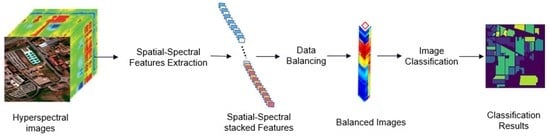
  • Proposing an innovative 1D_2D convolutional-based method for obtaining the spatial and spectral features from hyperspectral images. A 1D CNN network is adopted to extract the spectral features, whereas a 2D convolutional network is used to capture the spatial features. Finally, the two features are concatenated and stacked into one feature vector.
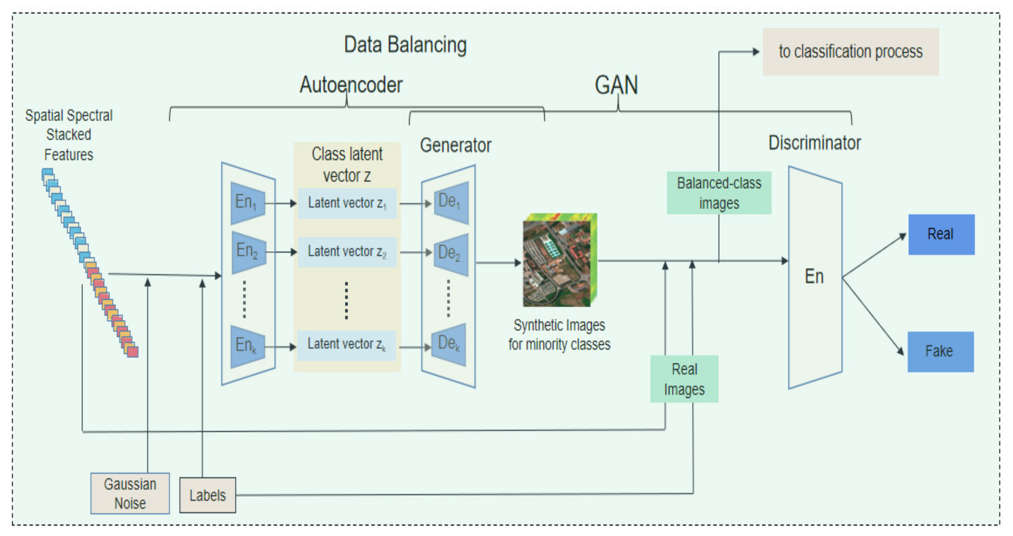
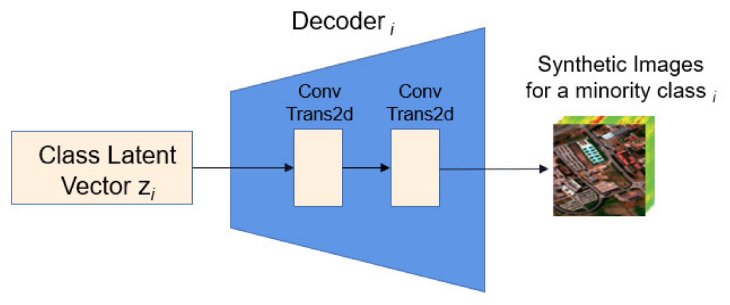
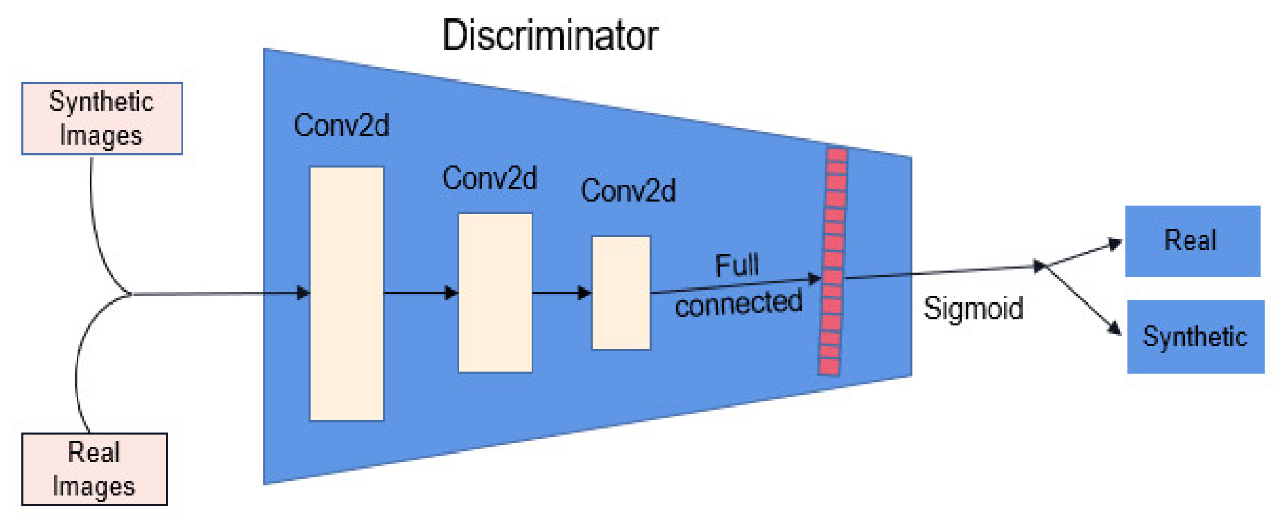
  • The autoencoder GAN-based model is proposed to solve the class imbalance issue, and synthetic images are generated to rebalance the minority classes and the datasets. Compared to the sample number in the majority class, an encoder cell would be determined and developed to produce samples for each minority class equal to the sample number in the majority class. The GAN model would be used to recognize the real samples and synthetic samples to enhance the results of the loss function, and improve the training convergence.
  • We introduce a simpler and more efficient way of HSI classification. A 2D CNN-based classifier is adopted for classifying hyperspectral images. The 2D convolutional network costs less time consumption and takes less space for the training process. The balanced images, including the synthetic and the real images, are fed into the proposed classifier for performing the image classification task.
  • Our model is validated using four hyperspectral datasets, including Salinas, Indian Pines, Botswana, and Kennedy Space Center. Our model is validated and compared with several state-of-the-art classifiers. Statistical significance is also estimated to examine classification performance obtained by the proposed model.
The remainder of this article is structured as following. In the next section, the related work is briefly reviewed. Section 3 describes our proposed model in detail. Experiment settings and information on datasets are illustrated in Section 4. The obtained results are presented in Section 5 and followed by the discussion in Section 6. Finally, the conclusions are summarized in Section 7.

2. Related Work

Many works in the literature address the class imbalance issue in HSI datasets. Here is a brief introduction to the research related to feature extraction, image generation, and classification for imbalanced data in HSI.

2.1. Feature Extraction Methods

The feature extraction process plays a vital role in HSI classification. A lot of methods have been proposed, and many approaches have been developed for enhancing classification performance. Convolutional neural networks have been considered for feature extraction approaches [11,12]. The automatic architecture of CNNs for the HSI classification was introduced in [13], which designed a 1D_3D Auto-CNN-based model to automatically obtain the features from the original image cube. The authors in [14] used a Gabor-filtering-based combination and a CNN-based model to obtain the spectral and spectral features, leading to a performance improvement. Zhang et al. [15] applied a 3D-based FractalNets method and the residual connections to extract the spatial–spectral features properly. Gao et al. [16] introduced a dual-branch-based feature extraction method along with an attention classification method for performing multiscale classification. The authors applied constructing multiple residual-like connections to assist in extracting the features at a granular level. Seydgar et al. [17] adopted ConvLSTM and 3D CNN methods to obtain the spatial–spectral features in HSI. Authors in [18,19] presented a 3D-CNN-based approach for HSI classification by applying 3D convolutional networks to properly obtain the spatial–spectral features.
Except for the CNN-based models, Vision-Transformer-related methods have become a new scheme for feature extraction in HSI. Dalal et al. [20] developed a transformation reduction (ETR) for reducing the dimensionality and classification complexity in HSI. Wang et al. [21] developed a Transformer network named UNetFormer for real-time urban scene segmentation and image classification. In [22], a bilateral awareness network for semantic segmentation was developed to increase the image resolution and improve the classification performance of HSI. In [23], a feature reduction method called improving distribution analysis (IDA) was developed for reducing data complexity and dimensionality of hyperspectral images. The correlation between related data is increased and the distance between big and small data is decreased, followed by increasing the value’s location inside the group range of the hyperspectral images.
Using the above studies’ feature extraction methods provided novel results for HSI classification can increase the classification accuracy. However, they lead to increases in the time consumed and the storage resources used, especially in the 3D CNN-based models. Thus, there is a need to develop a feature extraction strategy that can fully extract more valuable spatial and spectral features and alleviate the computational burden and time and storage resources.

2.2. Hyperspectral Image Classification on Imbalanced Data

For HSI classification, a lot of research used classical pattern recognition, machine learning, and deep-learning models.
In [24], the authors introduced a CNN patch-free-based method for classification. A CNN content-guided model was proposed for HSI classification. Roy et al. developed a novel model named HybridSN. The model can extract the spectral features and the spatial features by combining the 3D convolutions and the 2D convolutions with lightweight spatial–spectral residual features to reduce the parameters used for the sample training process of classification [25]. The authors in [26] presented a 3D coordination attention-based learning method for HSI classification. In that approach, the attention mechanism can obtain the long-distance dependence of horizontal directions, spatial position, and the important difference between various spectral bands. AL-Alimi et al. [27] proposed a hyperspectral image classification framework adopting a meta-learner method for training multi-class datasets using hybrid and multi-size kernel convolutional neural networks. Ma et al. [28] presented a spatial–spectral kernels-based generation network for producing spatial and spectral kernels using image characteristics, which were utilized to enhance the classification accuracy.
Although such outstanding results were obtained by previous models solving classification issues, there is a need to propose a new approach which can tackle the issue of the class imbalance in HSI datasets. The class imbalance issue can make the classification result biased toward learning the information from the majority classes and ignoring the minority classes [29]. The classification measures, such as overall accuracy (OA), and Kappa metric, etc., can be poorly presented for minority classes.
Several methods have been developed to address the class imbalance issue [30,31]. For example, sampling-based approaches are widely adopted due to their simple structure. These approaches are often adopted for preprocessing the imbalanced datasets before training to achieve better classification accuracy. Solving the imbalanced dataset approaches can be divided into two types, namely, undersampling and oversampling methods [32].
The undersampling-based methods mainly decrease the samples in the majority class to rebalance the samples in datasets. Singh et al. [33] proposed a SMOTE and centroid-based clustering method for undersampling the majority of class samples in the HSI datasets. In the study [34], a random feature subspace was used to perform an oversampling method for training samples and data enhancement. An ensemble-based learning model was developed by merging random feature selection with a convolutional network for performing image classification.
The oversampling-based methods increase the number of instances in the minority class by data augmenting or sample replication methods. For instance, Zhu et al. [35] adopted the GAN model to produce new samples for training the network and enhancing classification accuracy. In [36], a multiple-category spatial–spectral-based GAN approach was proposed. Two generator cells were utilized to extract the spectral features and the spatial features for the adversarial objectives for various classes. In [37], the authors introduced a new Caps-TripleGAN model to generate new images using a 1D_3D GAN and then classified the hyperspectral images using a capsule net-based model. Xue [38] presented a GAN-based image classification model using a 3D convolutional network and a 3D convolutional residual network. Roy et al. [39] developed a 3D adversarial oversampling-based model for HSI classification. The image samples were produced using a 3D hyperspectral patch. Then, a 3D-CNN-GAN-based classifier was used to perform the classification task.
Overall, although the above classification methods obtained outstanding results, the 3D convolution-based approaches have several drawbacks. For instance, with the growing number of 3D convolutions, the consumed time is getting longer. In addition, the overwhelming features can lead to an overfitting issue and influence the classification accuracy. Although the methods mentioned above adopted adversarial training for classification, they did not provide an effective solution for the minority classes. Therefore, there is still a need to produce image samples for each class and try to solve the class imbalance issue in HSI datasets.

3. The Proposed Model

This section introduces our model, and the detailed structure of the proposal is illustrated in Figure 1.
Our model contains three modules, namely, a feature extraction module, a data-balancing module, and a classification module. Firstly, the hyperspectral image size is reduced, then the main spectral features and the spatial features are extracted to understand the implicit feature distribution of the hyperspectral images. Secondly, the real images, represented by spatial–spectral features, are fed to an autoencoder module. The image labels are input with the minority class images, and a labeled latent vector is generated for each minority class. Thirdly, the GAN model receives the labeled latent vector, which represents the image features and the real images, then generates synthetic images and, in turn, recognizes the real images from the synthetic images. Finally, the balanced images are fed into the classification model for performing classification and obtaining classification results.

3.1. Feature Extraction

For better capturing the features of HSI, the feature extraction process considers three steps: spatial feature extraction, spectral feature extraction, and feature fusion. Figure 2 illustrates the feature extraction module.
Spatial features can play a vital role in the classification accuracy of HSI. As shown in Figure 2, spatial feature extraction begins with selecting the suitable spatial window size for the images. The original size of hyperspectral images (H × W × D, indicate height, width, and bands for an HSI) is considered, and images with a new spatial window would be selected (become M × N × D). Then, the new-sized images are fed to the latent convolutional layers as input data. The 2D convolutional neural networks capture spatial features using reduced-size images. Table 1 illustrates the parameter settings of the convolutional layers for spatial feature extraction.
The proposed module of spatial feature extraction contains six layers, and the structure design is described in Table 1. An output of an ith layer is represented by a feature map with different output channels, which is fed to the next layer. For the sake of further enhancing the performance, the Mish learning function is utilized instead of ReLU, as the Mish function presented more accurate results than ReLU [40]. Mish can be calculated as the following equation [40]:
Mish ( x ) = tanh   ( ln   ( 1 + e x ) )   ×   x
where x presents inputs, ln (·) indicates logarithmic function, whereas tanh (·) denotes the popular function calculated as in the following equation [40].
tanh ( x ) = e x e x e x + e x
Once the ith layer’s structure is a convolution layer, a 2D CNN-based operation is performed using kernel size 3 × 3 to obtain features and outputs a feature map Oi. This process can be calculated as function (3) [41]:
O i = σ ( O i 1 W i + b i )
where σ (·) represents the Mish activation function, and ∗ is the convolution operation. Moreover, Oi−1 is the previous layer output, whereas Wi and bi denote weights matrix and the bias term of the current layer i.
Once an ith layer is maxpooling, the input size of a feature map would be shortened by replacing a 2 × 2 sized neighborhood region with the region’s maximum value. The calculation process is performed as in Equation (4):
Oi = maxPool(Oi−1)
Once the ith layer is a full connected layer, the spatial features can be extracted and are ready for concatenating with spectral features. The spatial features are denoted as Featurespatial. Mathematically, this step can be calculated as in Equation (5):
Featurespatial=Ofull_connected =σ(Oi−1 ∗ Wi +bi)
Similar to the convolution layer above, Oi-1 denotes an output of the previous layer, whereas Wi and bi represent weights matrix and the bias term of the current layer i.
Regarding spectral feature extraction, the principal components analysis decreases the dimensions number of the spectral domain. The new size of hyperspectral images would be reduced (the original size, H × W × D, becomes H × W × B, indicating height, width, and bands). The spectral extraction and spatial extraction have similar architecture as they contain six layers. In addition, Mish activation is utilized as the learning function in the convolutional layers as well. The only different aspect to the spectral features extraction module is to avoid the complexity of commutation, 1D convolutional neural networks are used instead of 2D convolutional neural networks. Finally, the fully-connected layer provides the spectral features, denoted by Featurespectral.
For the sake of facilitating the classification process and enhancing the classification accuracy, the captured spatial features and the spectral features are required to be fused. Let Featurespatial={Sp1,Sp2,…,Spn} represent the extracted spatial features and Featurespectral={Spe1,Spe2,…,Spem} represent the captured spectral features of a pixel with b bands. Thus, a spatial–spectral feature (Featurespatial_spectral) of a pixel is generated by stacking the spectral feature vector Featurespectral with the spatial vector Featurespatial, which can be obtained by the following equation:
Featurespatial_spectral={Sp1,Sp2,…,Spn,Spe1,Spe2,…,Spem}
In this article, Featurespatial_spectral is used as the feature of real images which would be fed into the data-balancing module and the image classification module.

3.2. Data Balancing

HSI datasets are considered imbalanced data in which there are majority class and minority classes. The majority class contains the largest image samples, whereas minority classes have fewer samples. This can lead to biased results and reduce classification accuracy. Thus, balancing samples for minority classes becomes vital. With the widespread use of GAN and autoencoder deep learning models in HSI data augmentation, this article adopted these two models to produce synthetic images for balancing minority classes. Figure 3 describes the main features of the data-balancing module.

3.2.1. Autoencoder Network

As depicted in Figure 3, the autoencoder network contains two sub-networks: the encoder and the decoder. The aim of the encoder is to oversample the images (image features) of the minority classes by producing new samples, as depicted in Figure 3. The spatial–spectral stacked features, Gaussian noise, and class information (labels) are fed to the encoder network. The image class having the largest samples is considered as a majority class, whereas other classes are labeled as minority classes. Therefore, the images’ number of the majority class would be captured and used to generate images and balance the shortage in minority classes.
Suppose the training set has k minority classes. Thus, the encoder network should have k encoder cells, one Eni cell for each minority class i. Each Eni cell generates Gen_Imi samples, as Equation (7):
Gen_Imi = Imm − Imi
where Imm represents the samples number of majority class m and Imi for minority class i, i ∈ [1, k]. Therefore, each Eni cell has the following inputs (Gen_Imi, class label i, Gaussian noise, and spatial_spectral features of the class samples) and encodes them into a class latent vector zi. Figure 4. describes the internal architecture of an encoder cell.
The encoder cell contains two convolutions and two maxpoolings, which are two-dimensional cells. The initial encoded vector obtained by the encoder i is the following Equation (8):
zi = Eni(xi) = q(zi|xi)
where xi is the stacked features of the minority class i, considering the Gaussian noise and the class labeli. After calculating mean µ with covariance ε from the stacked features, the class latent vector zi is Equation (9) is generated by applying Equation (9) [42]:
zi = µi + r ∗ exp(εi)
After extracting the class latent vector zi for each minority class i, the corresponding decoder Dei would be triggered and fed by the label latent vector zi. Figure 5 describes the internal architecture of a decoder cell.
The encoder cell contains two transposed convolutions (two-dimensional cells). In the encoder and the decoder layers, the ReLU activation function is applied, and the Adam algorithm is chosen as the optimization function. The aim of the decoder Dei is to learn the training data distribution, then produce image samples.
x i = Dec ( z i ) = p ( x i | z i )
where x i ¯ is the generated samples from the label latent vector zi. Finally, we obtain a set of synthetic images for each minority class i.

3.2.2. Generative Adversarial Networks (GAN) Network

In general, the architecture of a GAN contains two subnetworks, namely, generator network and discriminator network. The generator network obtains image features and generates synthetic images. In contrast, the discriminator network obtains synthetic images, and distinguishes the synthetic images from the real images, and accordingly modifies the loss function until no difference can be found between generated and real images.
For the sake of decreasing the time complexity of implementing our model and for simplifying the model design with no influence on model functions, we consider the decoder network of the autoencoder module as the generator network of the GAN module. In addition, the decoder network generates image samples for minority classes, as the generator network should do in the GAN module. Thus, we focus on the discriminator network. Figure 6 illustrates the discriminator network design.
According to Figure 6, the discriminator network includes three convolution layers, and all of these layers are two-dimensional layers. The first and second layers apply the ReLU activation, whereas the last layer utilizes the sigmoid activation to distinguish image’ types (real or synthetic). More details about the 2D discriminator design are introduced in Table 2.
The discriminator network receives the synthetic images generated by the decoder network and the real images as the input data. With the synthetic and real images, each image class becomes balanced, can increase the classification results, and performs image classification well. Therefore, the balanced images, including synthetic and real images, would also be sent to the classification.

3.3. Classification Module

The classifier network plays a vital role in our proposed model because of the need to classify the whole balanced image samples (the synthetic and the real ones). Figure 7 describes the design of our classification network.
As depicted in Figure 7, the classifier network’s design is similar to the discriminator network, and the only difference is that the last convolution layer used the SoftMax function. The classifier network calculates the scores of each image class, which are later used to obtain the value of SoftMax loss. The training and testing process of the classification network are implemented as follows. Training samples of every balanced image class (the real images and the samples generated from the autoencoder module for the minority classes) were used to performing the classification process, and testing data is utilized for validating the classification accuracy for each classification model.

4. Experiment

This article aims to develop a classification model for HSI, considering the minority class issue in the image samples. Therefore, we use the autoencoder and the GAN model to generate samples, balance the image number for each minority class, and improve the classification performance.

4.1. Datasets

Our study used four hyperspectral imbalanced datasets [43] with various environmental settings to validate the performance of our model, including Indian Pines, Kennedy Space Center, Salinas, and Botswana. Here is a short description of the datasets.
  • The Indian Pines dataset is collected using the AVIRIS sensor in the Indian Pines area, Indiana. The dataset includes 224 bands with range wavelength of 0.4–2.5 × 10 −6 m. Image size is 145 × 145 pixels [43]. More details of the classes and samples of Indian Pines are listed Table 3 and displayed om Figure 8.
  • The Salinas dataset is collected using AVIRIS sensor in the Salinas area, California. The Salinas dataset includes 204 bands, and the image size is 512 × 217 pixels [43]. Table 4 introduces more details about the land cover classes along with samples in the Salinas dataset, whereas Figure 9 shows the ground truth map and pseudo color image by Salinas dataset.
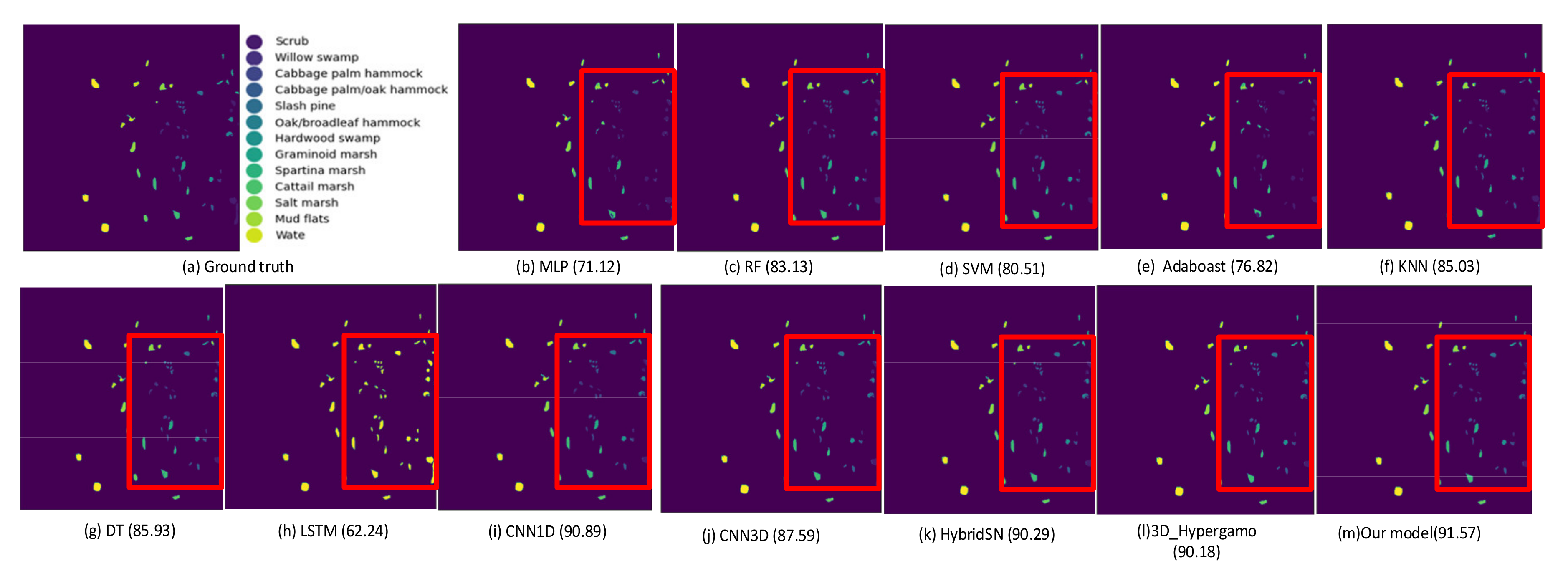
  • The Kennedy Space Center dataset is gathered using NASA AVIRIS at the Kennedy Space Center area in Florida. The KSC dataset contains 224 spectral reflectance bands, and image size is 512 × 614 pixels [43]. Table 5 listed the classes and the samples’ information of the KSC dataset, whereas the corresponding ground truth map and pseudo color image are depicted in Figure 10.
  • By NASA EO-1 satellite, the Botswana dataset is gathered across the Okavango delta site. The dataset includes 242 spectral reflectance bands, and the image size is 1496 × 256 pixels. Table 6 details the classes and the samples in the Botswana dataset. Figure 11 illustrates the ground truth map along with a pseudo color image for the Botswana dataset.

4.2. Experiment Settings

The experiments in this article were performed on a PC having Intel i7-10750 h with 32 GB RAM. RTX 2070 GeForce GPU with 11-GB memory. In addition, the Ubuntu 20 operating system was used for all experiments. Pytorch 1.11, cuDNN 8.4.1 and CUDA 11.3, matplotlib, and python 3.8 were the tool programming utilized in our experiments. All models performed by our experiments were applied on Anaconda 3.5 programming environment. Moreover, Earthpy, a transparent deep learning library, was used to provide for Earth dataset analytics. Platforms, such as TensorFlow, Keras, and Pandas, were combined into the core framework for processing and supporting the deep learning methods included in the proposed model.

4.3. Training Settings

The weights for the layers in our proposed model were randomly initialized, and the model parameters were updated by applying the Adam optimizer [44], along with a learning rate 0.0002. The maximum number of epochs was assigned to 400 for all datasets.
In our model’s training process, each experiment was run 4000 iterations, and once the generalization of the synthetic images of the minority classes became stable, the process terminated. A 25 × 25 × D spatial window was selected for the four datasets, where D represents the bands’ number.
Table 7 lists the distribution of training (Train) and synthetic samples (Synth), and the test samples (Test) of the four datasets. As shown in Table 7, the number of samples of the training and testing process were different for each dataset. For example, due to Indian Pines having the biggest number of samples, Soybean-mintill was considered the majority class. In the experiment, we considered 1500 samples as the sample number for the real training dataset. Other classes were considered minority classes that need to generate synthetic samples and rebalance the sample number of every minority class. The testing samples number considered 1/4 of the training samples for each dataset. The same settings were conducted for the classes in the other datasets, and more details are described in Table 7.

4.4. Comparation Models and Evaluation Metrics

For studying the effectiveness of our proposed model on imbalanced datasets, we conducted model comparisons over several traditional classifiers, such as MLP [44], RF [45], SVM [46], Ada Boost [47], KNN [48], and DT [49] over machine learning methods, including LSTM [50], CNN1D [51], and CNN3D [52], and over existing outstanding classifiers, such as HybridSN [25] and 3D_Hypergamo [39]. The HybridSN model combines 3D and 2D convolution models for HSI classification. The spatial–spectral features are extracted by 3D and 2D convolutions, respectively. The 3D_Hypergamo utilizes a 3D-generator network which contains conditional feature mapping units, namely 3D hyperspectral patches, to generate new samples for each class, and a 3D classifier is also used to classify the samples (real and generated) into the corresponding classes.
We estimate the classification performance using popular evaluation metrics, namely, overall accuracy (OA), average accuracy (AA), and the kappa metric. The OA metric is calculated by considering the ratio of classified correctly images against total samples number in the testing dataset. The AA metric denotes the mean of the accuracies of image class, whereas the kappa metric denotes the weighting of the measured accuracies. Therefore, we expect that the synthetic samples produced by our model enhanced the classification performance and resulted in higher accuracy when comparing with existing HSI classifiers.

5. Experimental Results

5.1. Classification Results with Compared Models

The classification results of our model are compared with existing outstanding classifiers by the train–test datasets of the four used datasets.
It needs to be mentioned that obtaining classification results by using only the information in the articles of classifiers or obtaining details of the codes and the implementations is very difficult. A lot of parameters and details of implementation were not found in the articles and could only be obtained by guess once regenerating the experimental results.
Table 8 reports a summary of the accuracy results of the classification models. It compares state-of-the-art models by various popular metrics. The highest values are marked with bold across all models.
As shown in Table 8, once comparing our model with classifier models using the four HSI datasets, our model achieves higher results regarding the metrics OA, AA, and kappa.
The Salinas dataset presents a larger spatial size and has the highest number of spectral bands; therefore, the obtained classification accuracy of Salinas is higher. Regarding the Indian Pines dataset, the spatial size is smaller along with sixteen classes, which leads to a lower accuracy performance. The Botswana dataset provides the highest spatial size among all HSI datasets, Botswana presents the least samples regarding the maps of ground truth. Thus, the accuracy results in the Botswana dataset are larger than those in the Indian Pines dataset and the Salinas dataset. The KSC dataset has only thirteen image classes, which can make the classification task easier than that in the other HSI datasets, and its overall classification accuracy is still high (reaches 91.57).
Regarding the Indian Pines dataset, our model achieves significant performance improvements of at least 1.3% and 1.1% regarding the OA and the kappa compared with the models: HybridSN, CNN3D, and 3D_ Hypergamo, as shown in Table 8. Traditional classifiers, such as RF and DT, achieved lower OA accuracy results (80.71 and 83.14), and LSTM achieved the lowest accuracy (60.22), which may show that LSTM networks are unsuitable for the image classification task. The CNN1D and CNN3D achieved high results (OA:93.31, 95.57, AA: 96.44, 95.57, and Kappa: 92.31, 93.89). These two models took advantage of rich information obtained by spectral features and spatial features and then enhanced the accuracy results.
In the Salinas dataset, DT shows the worst performance (OA: 79.24, AA: 66.54, and Kappa: 71.36), and FT and Ada Boost performed better than the DT model. The non-deep-learning-based approaches, i.e., SVM, KNN, and LSTM, obtained higher results. Moreover, the proposed model outperformed the deep-learning-based approaches (CNN3D, HybridSN, and 3D_ Hypergamo) and achieved a high level of 95.48%, 93.87%, 99.3%, and 94.01% for OA, AA, and kappa, respectively.
Our model significantly enhanced OA, AA, and kappa by about 2.7% compared to the second- and third-best models (HybridSN and 3D_Hypergamo) by the Botswana dataset. The worst results are recorded by Ada Boost and LSTM, ranging from 76.44–78.54 of OA, kappa, and AA. The remaining models achieved good results for the three metrics as well.
Regarding the KSC dataset, our model achieved the highest classification results on OA: 91.57 and kappa: 90.48, and the highest value of AA (86.45) was obtained by the CNN1D model. As expected, again, deep-learning-based approaches, such as CNN3D, HybridSN, and 3D_Hypergamo, obtained high accuracy results as these methods can effectively reduce overfitting, and the used parameters can update well during the backpropagation process.
In addition to the results of quantitative classification, classification maps of different classification models were investigated by data visualization. Figure 12, Figure 13, Figure 14 and Figure 15 illustrate classification maps generated by performing the HSI classifiers on the Indian Pine, Salinas, KSC, and Botswana datasets. The areas with different changes were marked using red triangles.
Regarding classification maps generated for Indian Pines, models with lower accuracy, i.e., RF, DT, and LSTM, resulted in observed scatter points in the classification maps, such as in Figure 12c,g,h.
In the Salinas dataset, Figure 13c,f,g illustrated dark scatter points as a result of the misclassification of a lot of points located at the center of land-cover areas by the classifiers, such as RF, Adaboost, and DT.
Figure 14 shows a comparation of classification maps across various classifiers performed on the KSC dataset. Figure 15b,e, and color-changed scatter points in Figure 14h show the effect of the misclassification of many points by MLP, Adaboost, and LSTM.
Similar results are also observed for the Botswana dataset, as shown in Figure 15. The classification maps produced by our model are obviously better than those generated by the other models.
The classification performance of the spatial–spectral-based classifiers can easily outperform other HSI models. CNN3D, HybridSN, and 3D_Hypergamo adopted deep networks to learn features, which resulted in smoother and higher-quality classification maps. The classification maps generated by deep-learning-based models show far higher quality compared to other methods.
By comparing the ground truth maps with classification maps, our model obtained the highest accuracy results on almost all HSI datasets and achieved significant qualitative enhancement compared to other maps as well. In addition, our model can also help to enhance the uniformity of the land-cover areas as depicted in Figure 12, Figure 13, Figure 14 and Figure 15.
The results prove that our model enhances the feature extraction and training processes and obviously outperforms the other classifiers well.

5.2. Training and Complexity Time with the Compared Models

Figure 16 shows the classification accuracy and loss comparisons for 100 epochs for training and validation.
As shown in Figure 16, our model performs convergence slower than the HybridSN but faster than the 3D_Hypergamo. The proposed model converged at about 30 epochs, whereas the HybridSN and 3D_Hypergamo converged at about 40. The HybridSN method achieves faster results as its simple design of an internal network has three 3D CNN layers and one 2D CNN layer. The 3D_Hypergamo model has a GAN-based network that needs settings for a huge amount of hyperparameters, which slows the convergence. In our study, our model adopted an autoencoder and GAN-based network, leading to an acceptable convergence speed. Compared with the HybridSN model, our model required analysis and learning more parameters, leading to slower convergence.
A comparison of the efficiency computation in terms of training and testing times of our model along with HybridSN and 3D_ Hypergamo is listed in Table 9. Our proposed model outperformed other models and needs less training time and testing time when compared to models HybridSN and 3D_Hypergamo.
Table 10 shows the spatial dimension’s impact on our model’s performance on the four datasets. The 25 × 25 spatial dimensions obviously achieve better results and become the most suitable for the proposed model.

6. Discussion

By analyzing the results achieved by the experiments above, several conclusions are drawn as follows.
Firstly, 1D CNN and 2D CNN-based networks can achieve better results in feature extraction compared to other models, such as Ada Boost [47], LSTM [50], CNN1D [51], HybridSN [25], and 3D_Hypergamo [39], as listed in Table 10. Our approach applied 1D convolutional networks and 2D convolutional networks to obtain the spatial and the spectral features of HSI. Using 1D convolutional networks to properly extract rich spectral features, the learning process becomes more effective and easier to implement. In addition, PCA is utilized to decrease spectral dimensionality to a smaller size, reducing the time consumed for learning features information. A larger spatial window size (25 × 25) is used over a 2D convolutional network for extracting spatial features and obtaining rich information attributed to HSI, then increase the classification accuracy as shown in Table 10.
Secondly, an autoencoder-GAN-based model was adopted to generate new sample models and to rebalance image class samples. The autoencoder model was applied to generate synthetic samples for each minority class in HSI datasets. An encoder and decoder cell were dedicated to a specific minority class, and the generated samples can be validated and modified using the discriminator network in the GAN network. Therefore, the samples in the minority classes would be rebalanced, and the sample number could be the same as the majority class, which leads to better results, as we can find in Table 10 and Figure 12, Figure 13, Figure 14 and Figure 15.
Thirdly, deep-learning-based approaches, especially CNN-based approaches, achieved higher classification accuracy results than traditional classifiers, such as MLP [44], RF [45], SVM [46], Ada Boost [47], KNN [48], etc. This may be due to the deep networks applied for the training and testing. Models, such as HybridSN [25] and 3D_ Hypergamo [39], and our approach obtained the highest classification results. All these models designed deeper CNN models for extracting features and then efficiently learning these features.
Finally, our model can achieve the highest value of classification accuracy on four used datasets, visually producing cleaner image classification maps, as the mistaken pixel number is remarkably reduced.

7. Conclusions

This study presents a hypered deep-learning-based HSI generation and classification model for imbalanced data. The proposed model provides an oversampling approach for solving class imbalance issues. Our model has three modules, namely, a feature extraction module, a data-balancing module, and a classification module. In the feature extraction module, spatial feature extraction begins with the principal components analysis method to decrease the spatial domain dimensions. The PCA method is followed by a 2D CNN that captures spatial features. Regarding spectral feature extraction, a 1D CNN was adopted to extract HSI spatial features, and the process of two feature extractions was performed synchronously. The two obtained features were fused into one spatial–spectral feature vector for improving image generation and classification.
GAN and autoencoder deep learning models in the data-balancing module were applied to produce synthetic images for balancing minority classes. Using the GAN structure, an encoder cell and a decoder cell were constructed for each minority class to generate and compensate new images, rebalance the samples, and increase the samples number to be the same as in the related majority class. A 2D CNN-based classifier was adopted to categorize the balanced, synthetic, and real samples.
The proposed model was validated using four open-access datasets. The results were compared with existing outstanding HSI classifiers. The results of our model outperformed the other classifiers in most cases. Moreover, the performance of our model is more suitable for imbalanced sets. The classification maps visualized by our proposed model were more suitable and smoother than those generated by other classifiers.
Overall, the proposed oversampling approach on minority classes led our proposed approach to extract more relevant features from various image classes, enhance the classification results, and improve remote sensing applications.
In future work, we need to perform more efforts in the following promising research fields. Firstly, besides developing oversampling techniques for HSI classification, there is a need to consider undersampling techniques to tackle the imbalance of data issues for HSI classification. Secondly, we need to study the classification problem in a large-scale benchmark dataset and investigate the classification performance of the hyperspectral images. The existing datasets may not be enough for studying the HSI classification issue. Finally, image decompression is another research field that needs to be considered, as image decompression can reduce the time needed for the classification task.

Author Contributions

Conceptualization, H.A.H.N.; methodology H.A.H.N.; data curation, T.L.; writing—original draft preparation, H.A.H.N.; formal analysis, Q.X.; investigation, T.L.; writing—review and editing, X.D.; visualization, Q.X.; supervision, T.L.; project administration, T.L., Q.X. All authors have read and agreed to the published version of the manuscript.

Funding

This research received no external funding.

Data Availability Statement

All the datasets are available at this link: http://www.ehu.eus/ccwintco/index.php/Hyperspectral_Remote_Sensing_Scenes, accessed on 6 May 2022.

Conflicts of Interest

All authors declared no conflict of interest.

References

  1. Zhang, M.; Li, W.; Du, Q. Diverse Region-Based CNN for Hyperspectral Image Classification. IEEE Trans. Image Process. 2018, 27, 2623–2634. [Google Scholar] [CrossRef] [PubMed]
  2. Ghamisi, P.; Plaza, J.; Chen, Y.; Li, J.; Plaza, A.J. Advanced Spectral Classifiers for Hyperspectral Images: A review. IEEE Geosci. Remote Sens. Mag. 2017, 5, 8–32. [Google Scholar] [CrossRef] [Green Version]
  3. Li, J.; Du, Q.; Li, Y.; Li, W. Hyperspectral Image Classification with Imbalanced Data Based on Orthogonal Complement Subspace Projection. IEEE Trans. Geosci. Remote Sens. 2018, 56, 3838–3851. [Google Scholar] [CrossRef]
  4. Li, S.; Song, W.; Fang, L.; Chen, Y.; Ghamisi, P.; Benediktsson, J.A. Deep Learning for Hyperspectral Image Classification: An Overview. IEEE Trans. Geosci. Remote Sens. 2019, 57, 6690–6709. [Google Scholar] [CrossRef] [Green Version]
  5. Wambugu, N.; Chen, Y.; Xiao, Z.; Tan, K.; Wei, M.; Liu, X.; Li, J. Hyperspectral image classification on insufficient-sample and feature learning using deep neural networks: A review. Int. J. Appl. Earth Obs. Geoinf. 2021, 105, 102603. [Google Scholar] [CrossRef]
  6. Gao, H.; Chen, Z.; Xu, F. Adaptive spectral-spatial feature fusion network for hyperspectral image classification using limited training samples. Int. J. Appl. Earth Obs. Geoinf. 2022, 107, 102687. [Google Scholar] [CrossRef]
  7. Xu, Y.; Du, B.; Zhang, L. Beyond the Patchwise Classification: Spectral-Spatial Fully Convolutional Networks for Hyperspectral Image Classification. IEEE Trans. Big Data 2019, 6, 492–506. [Google Scholar] [CrossRef]
  8. Naji, H.A.H.; Xue, Q.; Lyu, N.; Duan, X.; Li, T. Risk Levels Classification of Near-Crashes in Naturalistic Driving Data. Sustainability 2022, 14, 6032. [Google Scholar] [CrossRef]
  9. Naji, H.A.H.; Xue, Q.; Zhu, H.; Li, T. Forecasting Taxi Demands Using Generative Adversarial Networks with Multi-Source Data. Appl. Sci. 2021, 11, 9675. [Google Scholar] [CrossRef]
  10. Jia, S.; Jiang, S.; Lin, Z.; Li, N.; Xu, M.; Yu, S. A survey: Deep learning for hyperspectral image classification with few labeled samples. Neurocomputing 2021, 448, 179–204. [Google Scholar] [CrossRef]
  11. Khan, S.; Rahmani, H.; Shah, S.A.A.; Bennamoun, M. A Guide to Convolutional Neural Networks for Computer Vision. Synth. Lect. Comput. Vis. 2018, 8, 1–207. [Google Scholar] [CrossRef]
  12. He, N.; Paoletti, M.E.; Haut, J.N.M.; Fang, L.; Li, S.; Plaza, A.; Plaza, J. Feature Extraction with Multiscale Covariance Maps for Hyperspectral Image Classification. IEEE Trans. Geosci. Remote Sens. 2018, 57, 755–769. [Google Scholar] [CrossRef]
  13. Chen, Y.; Zhu, K.; Zhu, L.; He, X.; Ghamisi, P.; Benediktsson, J.A. Automatic Design of Convolutional Neural Network for Hyperspectral Image Classification. IEEE Trans. Geosci. Remote Sens. 2019, 57, 7048–7066. [Google Scholar] [CrossRef]
  14. Chen, Y.; Zhu, L.; Ghamisi, P.; Jia, X.; Li, G.; Tang, L. Hyperspectral Images Classification with Gabor Filtering and Convolutional Neural Network. IEEE Geosci. Remote Sens. Lett. 2017, 14, 2355–2359. [Google Scholar] [CrossRef]
  15. Zhang, X.; Wang, Y.; Zhang, N.; Xu, D.; Luo, H.; Chen, B.; Ben, G. Spectral–Spatial Fractal Residual Convolutional Neural Network with Data Balance Augmentation for Hyperspectral Classification. IEEE Trans. Geosci. Remote Sens. 2021, 59, 10473–10487. [Google Scholar] [CrossRef]
  16. Gao, H.; Zhang, Y.; Chen, Z.; Li, C. A Multiscale Dual-Branch Feature Fusion and Attention Network for Hyperspectral Images Classification. IEEE J. Sel. Top. Appl. Earth Obs. Remote Sens. 2021, 14, 8180–8192. [Google Scholar] [CrossRef]
  17. Seydgar, M.; Naeini, A.A.; Zhang, M.; Li, W.; Satari, M. 3-D Convolution-Recurrent Networks for Spectral-Spatial Classification of Hyperspectral Images. Remote Sens. 2019, 11, 883. [Google Scholar] [CrossRef] [Green Version]
  18. Chen, Y.; Jiang, H.; Li, C.; Jia, X.; Ghamisi, P. Deep Feature Extraction and Classification of Hyperspectral Images Based on Convolutional Neural Networks. IEEE Trans. Geosci. Remote Sens. 2016, 54, 6232–6251. [Google Scholar] [CrossRef] [Green Version]
  19. Hamida, A.B.; Benoit, A.; Lambert, P.; Amar, C.B. 3-D deep learning approach for remote sensing image classification. IEEE Trans. Geosci. Remote Sens. 2018, 56, 4420–4434. [Google Scholar] [CrossRef] [Green Version]
  20. Al-Alimi, D.; Cai, Z.; Al-Qaness, M.A.; Alawamy, E.A.; Alalimi, A. ETR: Enhancing transformation reduction for reducing dimensionality and classification complexity in hyperspectral images. Expert Syst. Appl. 2023, 213, 118971. [Google Scholar] [CrossRef]
  21. Wang, L.; Li, R.; Zhang, C.; Fang, S.; Duan, C.; Meng, X.; Atkinson, P.M. UNetFormer: A UNet-like transformer for efficient semantic segmentation of remote sensing urban scene imagery. ISPRS J. Photogramm. Remote Sens. 2022, 190, 196–214. [Google Scholar] [CrossRef]
  22. Wang, L.; Li, R.; Wang, D.; Duan, C.; Wang, T.; Meng, X. Transformer Meets Convolution: A Bilateral Awareness Network for Semantic Segmentation of Very Fine Resolution Urban Scene Images. Remote Sens. 2021, 13, 3065. [Google Scholar] [CrossRef]
  23. Al-Alimi, D.; Al-Qaness, M.A.; Cai, Z.; Alawamy, E.A. IDA: Improving distribution analysis for reducing data complexity and dimensionality in hyperspectral images. Pattern Recognit. 2023, 134, 109096. [Google Scholar] [CrossRef]
  24. Zheng, Z.; Zhong, Y.; Ma, A.; Zhang, L. FPGA: Fast Patch-Free Global Learning Framework for Fully End-to-End Hyperspectral Image Classification. IEEE Trans. Geosci. Remote Sens. 2020, 58, 5612–5626. [Google Scholar] [CrossRef]
  25. Roy, S.K.; Krishna, G.; Dubey, S.R.; Chaudhuri, B.B. HybridSN: Exploring 3-D–2-D CNN Feature Hierarchy for Hyperspectral Image Classification. IEEE Geosci. Remote Sens. Lett. 2020, 17, 277–281. [Google Scholar] [CrossRef] [Green Version]
  26. Shi, C.; Liao, D.; Zhang, T.; Wang, L. Hyperspectral Image Classification Based on 3D Coordination Attention Mechanism Network. Remote Sens. 2022, 14, 608. [Google Scholar] [CrossRef]
  27. Al-Alimi, D.; Al-Qaness, M.A.A.; Cai, Z.; Dahou, A.; Shao, Y.; Issaka, S. Meta-Learner Hybrid Models to Classify Hyperspectral Images. Remote Sens. 2022, 14, 1038. [Google Scholar] [CrossRef]
  28. Ma, W.; Ma, H.; Zhu, H.; Li, Y.; Li, L.; Jiao, L.; Hou, B. Hyperspectral image classification based on spatial and spectral kernels generation network. Inf. Sci. 2021, 578, 435–456. [Google Scholar] [CrossRef]
  29. Shamsolmoali, P.; Zareapoor, M.; Shen, L.; Sadka, A.H.; Yang, J. Imbalanced data learning by minority class augmentation using capsule adversarial networks. Neurocomputing 2020, 459, 481–493. [Google Scholar] [CrossRef]
  30. Du, J.; Zhou, Y.; Liu, P.; Vong, C.-M.; Wang, T. Parameter-Free Loss for Class-Imbalanced Deep Learning in Image Classification. IEEE Trans. Neural Networks Learn. Syst. 2021, 1–7. [Google Scholar] [CrossRef]
  31. Huang, Y.; Jin, Y.; Li, Y.; Lin, Z. Towards Imbalanced Image Classification: A Generative Adversarial Network Ensemble Learning Method. IEEE Access 2020, 8, 88399–88409. [Google Scholar] [CrossRef]
  32. Özdemir, A.; Polat, K.; Alhudhaif, A. Classification of imbalanced hyperspectral images using SMOTE-based deep learning methods. Expert Syst. Appl. 2021, 178, 114986. [Google Scholar] [CrossRef]
  33. Singh, P.S.; Singh, V.P.; Pandey, M.K.; Karthikeyan, S. Enhanced classification of hyperspectral images using improvised oversampling and undersampling techniques. Int. J. Inf. Technol. 2022, 14, 389–396. [Google Scholar] [CrossRef]
  34. Lv, Q.; Feng, W.; Quan, Y.; Dauphin, G.; Gao, L.; Xing, M. Enhanced-Random-Feature-Subspace-Based Ensemble CNN for the Imbalanced Hyperspectral Image Classification. IEEE J. Sel. Top. Appl. Earth Obs. Remote Sens. 2021, 14, 3988–3999. [Google Scholar] [CrossRef]
  35. Zhu, L.; Chen, Y.; Ghamisi, P.; Benediktsson, J.A. Generative Adversarial Networks for Hyperspectral Image Classification. IEEE Trans. Geosci. Remote Sens. 2018, 56, 5046–5063. [Google Scholar] [CrossRef]
  36. Feng, J.; Yu, H.; Wang, L.; Cao, X.; Zhang, X.; Jiao, L. Classification of Hyperspectral Images Based on Multiclass Spatial–Spectral Generative Adversarial Networks. IEEE Trans. Geosci. Remote Sens. 2019, 57, 5329–5343. [Google Scholar] [CrossRef]
  37. Wang, X.; Tan, K.; Du, Q.; Chen, Y.; Du, P. Caps-TripleGAN: GAN-assisted CapsNet for hyperspectral image classification. IEEE Trans. Geosci. Remote Sens. 2019, 57, 7232–7245. [Google Scholar] [CrossRef]
  38. Xue, Z. Semi-supervised convolutional generative adversarial network for hyperspectral image classification. IET Image Process. 2020, 14, 709–719. [Google Scholar] [CrossRef]
  39. Roy, S.K.; Haut, J.M.; Paoletti, M.E.; Dubey, S.R.; Plaza, A. Generative Adversarial Minority Oversampling for Spectral–Spatial Hyperspectral Image Classification. IEEE Trans. Geosci. Remote Sens. 2022, 60, 1–15. [Google Scholar] [CrossRef]
  40. Mish, M.D. A self-regularized non-monotonic neural activation function. arXiv 2019, arXiv:1908.08681. [Google Scholar]
  41. Ge, Z.; Cao, G.; Li, X.; Fu, P. Hyperspectral Image Classification Method Based on 2D–3D CNN and Multibranch Feature Fusion. IEEE J. Sel. Top. Appl. Earth Obs. Remote Sens. 2020, 13, 5776–5788. [Google Scholar] [CrossRef]
  42. Chen, Z.; Tong, L.; Qian, B.; Yu, J.; Xiao, C. Self-Attention-Based Conditional Variational Auto-Encoder Generative Adversarial Networks for Hyperspectral Classification. Remote Sens. 2021, 13, 3316. [Google Scholar] [CrossRef]
  43. Hyperspectral Remote Sensing Scenes. Available online: https://www.ehu.eus/ccwintco/index.php/Hyperspectral_Remote_Sensing_Scenes (accessed on 6 May 2022).
  44. Meng, Z.; Zhao, F.; Liang, M. SS-MLP: A Novel Spectral-Spatial MLP Architecture for Hyperspectral Image Classification. Remote Sens. 2021, 13, 4060. [Google Scholar] [CrossRef]
  45. Melgani, F.; Bruzzone, L. Classification of hyperspectral remote sensing images with support vector machines. IEEE Trans. Geosci. Remote Sens. 2004, 42, 1778–1790. [Google Scholar] [CrossRef] [Green Version]
  46. Svetnik, V.; Liaw, A.; Tong, C.; Culberson, J.C.; Sheridan, R.P.; Feuston, B.P. Random Forest: A Classification and Regression Tool for Compound Classification and QSAR Modeling. J. Chem. Inf. Comput. Sci. 2003, 43, 1947–1958. [Google Scholar] [CrossRef]
  47. Li, L.; Wang, C.; Li, W.; Chen, J. Hyperspectral image classification by AdaBoost weighted composite kernel extreme learning machines. Neurocomputing 2018, 275, 1725–1733. [Google Scholar] [CrossRef]
  48. Tu, B.; Wang, J.; Kang, X.; Zhang, G.; Ou, X.; Guo, L. KNN-Based Representation of Superpixels for Hyperspectral Image Classification. IEEE J. Sel. Top. Appl. Earth Obs. Remote Sens. 2018, 11, 4032–4047. [Google Scholar] [CrossRef]
  49. Hao, S. Application of PCA dimensionality reduction and decision tree in hyperspectral image classification. Comput. Era 2017, 5, 40–43. [Google Scholar]
  50. Zhou, F.; Hang, R.; Liu, Q.; Yuan, X. Hyperspectral image classification using spectral-spatial LSTMs—ScienceDirect. Neurocomputing 2019, 328, 39–47. [Google Scholar] [CrossRef]
  51. Hu, W.; Huang, Y.; Wei, L.; Zhang, F.; Li, H. Deep Convolutional Neural Networks for Hyperspectral Image Classification. J. Sens. 2015, 2015, 258619. [Google Scholar] [CrossRef] [Green Version]
  52. Li, Y.; Zhang, H.; Shen, Q. Spectral–Spatial Classification of Hyperspectral Imagery with 3D Convolutional Neural Network. Remote Sens. 2017, 9, 67. [Google Scholar] [CrossRef]
Figure 1. Architecture of the proposed model.
Remotesensing 14 06406 g001
Figure 2. The architecture of the feature extraction module.
Remotesensing 14 06406 g002
Figure 3. The data balancing module with autoencoder and GAN.
Remotesensing 14 06406 g003
Figure 4. The internal architecture of an encoder cell.
Remotesensing 14 06406 g004
Figure 5. The internal architecture of a decoder cell.
Remotesensing 14 06406 g005
Figure 6. The illustration of the discriminator network.
Remotesensing 14 06406 g006
Figure 7. Design of our classification network.
Remotesensing 14 06406 g007
Figure 8. Indian Pines dataset: (a) ground truth map; (b) pseudo color image.
Remotesensing 14 06406 g008
Figure 9. Salinas dataset: (a) ground truth map; (b) pseudo color image.
Remotesensing 14 06406 g009
Figure 10. (a) Ground truth map; (b) false color image of KSC.
Remotesensing 14 06406 g010
Figure 11. (a) Ground truth; (b) false color image for Botswana dataset.
Remotesensing 14 06406 g011
Figure 12. Classification maps of the real and synthetic Indian Pines dataset by classification models.
Remotesensing 14 06406 g012
Figure 13. Classification maps of the real and synthetic Salinas dataset by classification models.
Remotesensing 14 06406 g013
Figure 14. Classification maps of the real and synthetic KSC dataset by classification models.
Remotesensing 14 06406 g014
Figure 15. Classification maps of the real and synthetic Botswana dataset by classification models.
Remotesensing 14 06406 g015
Figure 16. Accuracy and loss convergence versus epochs of three models.
Remotesensing 14 06406 g016
Table 1. The parameters setting of convolution layers for spatial feature extraction.
LayerInput ChannelsOutput ChannelsKernel SizePrevious Layer
Input11
2D CNN 11323 × 3Input
carpooling 132322 × 22D CNN 1
2D CNN 232643 × 3carpooling 1
maxpooling 264642 × 22D CNN 2
2D CNN 3645123 × 3maxpooling 2
FullConnected 2D CNN 3
Table 2. Parameters setting of convolution layers for the discriminator network.
LayerInput ChannelsOutput ChannelsKernel SizePrevious Layer
2D Conv_132323 × 3
2D Conv_232643 × 32D Conv_1
2D Conv_3645123 × 32D Conv_2
FullConnected 2D Conv_3
Table 3. Classes information of Indian Pines dataset.
NumberLand Cover ClassSamples
1Alfalfa46
2Corn notill1428
3Corn-mintill830
4Corn237
5Grass-pasture483
6Grass-trees730
7Grass-pasture-mowed28
8Hay-windrowed478
9Oats20
10Soybean-notill972
11Soybean-mintill2455
12Soybean-clean593
13Wheat205
14Woods1265
15Buildings Grass Trees-Drives386
16Stone-Steel-Towers93
Table 4. Classes information of Salinas dataset.
NumberLand Cover ClassSamples
1Brocoli_green_weeds_12009
2Brocoli_green_weeds_23726
3Fallow1976
4Fallow_rough_plow1394
5Fallow_smooth2678
6Stubble3959
7Celery3579
8Grapes_untrained11,271
9Soil_vinyard_develop6203
10Corn_senesced_green_weeds3278
11Lettuce_romaine_4wk1068
12Lettuce_romaine_5wk1927
13Lettuce_romaine_6wk916
14Lettuce_romaine_7wk1070
15Vinyard_untrained7268
16Vinyard_vertical_trellis1807
Table 5. Classes information of KSC dataset.
NumberLand Cover ClassSamples
1Scrub761
2Willow swamp243
3CP hammock256
4Slash Pine252
5Oak/Broadleaf161
6Hardwood229
7Swap105
8Graminoid marsh431
9Spartina marsh520
10Cattail marsh404
11Salt marsh419
12Mud flats503
13Water927
Table 6. Classes information of the Botswana dataset.
NumberLand Cover ClassSamples
1Water270
2Hippo Grass101
3Floodplain Grasses1251
4Floodplain Grasses2215
5Reeds1269
6Riparian269
7Firescar2259
8Island interior203
9Accacia woodlands314
10Accacia grasslands248
11Short mopane305
12Mixed mopane181
13Exposed soils268
Table 7. Samples information of the training and testing process of four datasets.
NoIndian PinesSalinaKSCBotswana
TrainTestTrainTestTrainTestTrainTest
RealSynthTotalRealSynthTotalRealSynthTotalRealSynthTotal
1461454150037520095491750018757611399002252705032080
21428721500375372637747500187524365790022510121932080
3830670150037519765524750018752566449002252516932080
423712631500375139461067500187525264890022521510532080
54831017150037526784822750018751617399002252695132080
6730770150037539593541750018752296719002252695132080
7281472150037535793921750018751057959002252596132080
847810221500375750007500187543146990022520311732080
920148015003756203129775001875520380900225314632080
10972528150037532784222750018754044969002252487232080
1115000150037510686432750018754194819002253051532080
125939071500375192755737500187550339790022518113932080
13205129515003759166584750018759000900225
14126523515003751070643075001875
1538611141500375726823275001875
1693140715003751807569375001875
Table 8. Comparison of classification performance of the compared models and our model.
MethodIndian PinesSalinasBotswanaKSC
OAAAKappaOAAAKappaOAAAKappaOAAAKappa
MLP [44]90.2193.1188.7292.1788.3889.5980.3480.1978.6771.1272.7975.58
RF [45]83.1485.1581.1483.6381.2378.3283.5984.9982.2383.1376.7681.17
SVM [46]88.3293.7587.5086.3684.1981.9586.2587.1685.1080.5179.1578.89
Ada Boost [47]92.7496.4392.4483.8071.2977.6978.5477.8776.7176.8277.9578.12
KNN [48]91.1695.1689.1589.2386.8685.4989.7990.6588.9485.0378.8383.30
DT [49]80.7183.1480.1479.2466.5471.3689.8890.7989.0485.9379.8684.31
LSTM [50]60.2258.5159.6891.6388.3888.878.2977.7276.4462.2462.0063.24
CNN1D [51]93.3196.4492.3192.0289.3889.3189.5790.7588.7190.8986.4589.85
CNN3D [52]94.0495.5793.8991.5688.388.7186.2987.1885.1587.5982.0886.17
HybridSN [25]92.3495.3691.4695.0793.693.4690.2391.3789.4290.2985.0689.18
3D_Hyperamo [39]94.2494.6493.6993.7191.0891.5694.2294.8193.7490.1885.0289.06
Our model94.4794.9294.0995.4893.8794.0196.7496.3196.5791.5786.4290.48
Table 9. Training in minutes and testing in seconds over the four datasets by the compared models.
DatasetHybridSN3D_HypergamoOur Model
Training (mins)Testing (sec)Training (mins)Testing (sec)Training (mins)Testing (sec)
Indian Pines2.32.12.62.12.21.8
Salinas3.12.93.23.23.63.25
KSC2.631.92.82.913.72.81
Botswana3.12.93.342.52.72.18
Table 10. Comparison of the performance of our model with different spatial windows sizes.
WindowIndian Pines (%)Salinas (%)KSC (%)Botswana (%)
19 × 1995.3295.8295.3895.89
21 × 2196.8796.1996.7397.83
23 × 2397.9297.4596.6697.38
25 × 2598.2299.1199.6299.78
Publisher’s Note: MDPI stays neutral with regard to jurisdictional claims in published maps and institutional affiliations.

