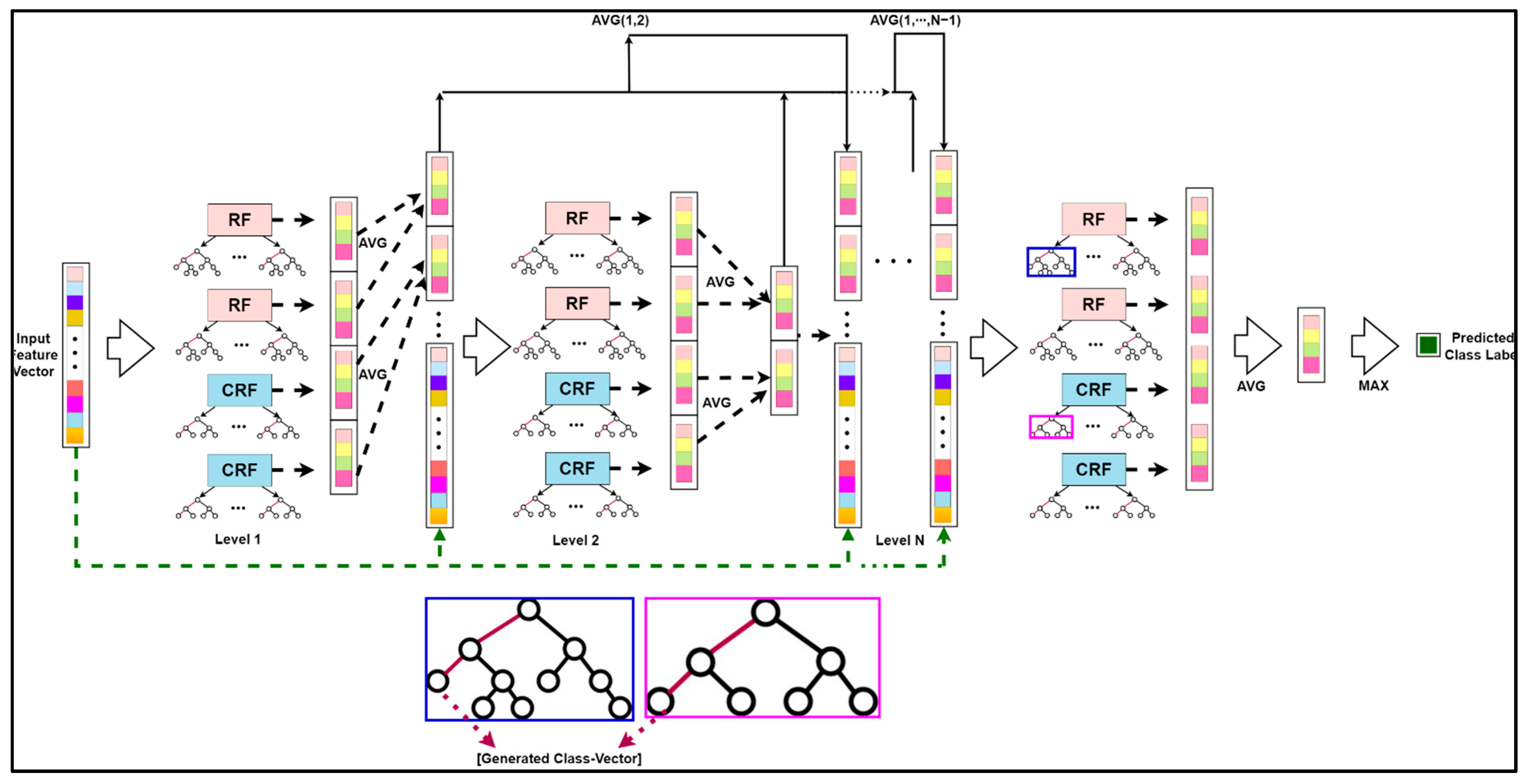
Article

A Hybrid Classification of Imbalanced Hyperspectral Images Using ADASYN and Enhanced Deep Subsampled Multi-Grained Cascaded Forest

by
Debaleena Datta
1,
Pradeep Kumar Mallick
1,
Annapareddy V. N. Reddy
2,
Mazin Abed Mohammed
3,
Mustafa Musa Jaber
4,5,
Abed Saif Alghawli
6,* and
Mohammed A. A. Al-qaness
7,8
1
School of Computer Engineering, Kalinga Institute of Industrial Technology, Deemed to be University, Bhubaneswar 751024, Odisha, India
2
Lakireddy Bali Reddy College of Engineering, Mylavaram 521230, Andhra Predesh, India
3
College of Computer Science and Information Technology, University of Anbar, Anbar 31001, Iraq
4
Department of Computer Science, Dijlah University College, Baghdad 00964, Iraq
5
Department of Computer Science, Al-Turath University College, Baghdad 10021, Iraq
6
Computer Science Department, College of Sciences and Humanities, Prince Sattam bin Abdulaziz University, Al-Kharj 16278, Saudi Arabia
7
College of Physics and Electronic Information Engineering, Zhejiang Normal University, Jinhua 321004, China
8
Faculty of Engineering, Sana’a University, Sana’a 12544, Yemen
*
Author to whom correspondence should be addressed.
Remote Sens. 2022, 14(19), 4853; https://doi.org/10.3390/rs14194853
Submission received: 25 July 2022 / Revised: 21 September 2022 / Accepted: 24 September 2022 / Published: 28 September 2022

Abstract

:
Hyperspectral image (HSI) analysis generally suffers from issues such as high dimensionality, imbalanced sample sets for different classes, and the choice of classifiers for artificially balanced datasets. The existing conventional data imbalance removal techniques and forest classifiers lack a more efficient approach to dealing with the aforementioned issues. In this study, we propose a novel hybrid methodology ADASYN-enhanced subsampled multi-grained cascade forest (ADA-Es-gcForest) which comprises four folds: First, we extracted the most discriminative global spectral features by reducing the vast dimensions, i.e., the redundant bands using principal component analysis (PCA). Second, we applied the subsampling-based adaptive synthetic minority oversampling method (ADASYN) to augment and balance the dataset. Third, we used the subsampled multi-grained scanning (Mg-sc) to extract the minute local spatial–spectral features by adaptively creating windows of various sizes. Here, we used two different forests—a random forest (RF) and a complete random forest (CRF)—to generate the input joint-feature vectors of different dimensions. Finally, for classification, we used the enhanced deep cascaded forest (CF) that improvised in the dimension reduction of the feature vectors and increased the connectivity of the information exchange between the forests at the different levels, which elevated the classifier model’s accuracy in predicting the exact class labels. Furthermore, the experiments were accomplished by collecting the three most appropriate, publicly available his landcover datasets—the Indian Pines (IP), Salinas Valley (SV), and Pavia University (PU). The proposed method achieved 91.47%, 98.76%, and 94.19% average accuracy scores for IP, SV, and PU datasets. The validity of the proposed methodology was testified against the contemporary state-of-the-art eminent tree-based ensembled methods, namely, RF, rotation forest (RoF), bagging, AdaBoost, extreme gradient boost, and deep multi-grained cascade forest (DgcForest), by simulating it numerically. Our proposed model achieved correspondingly higher accuracies than those classifiers taken for comparison for all the HS datasets.

1. Introduction

The spatial–spectral resolution of HSI has substantially improved with the speedy expansion of earth-observation technologies. Over the past two decades, they have been used in several applications for the advancement of humanity, such as the management of the environment [1], agricultural precision [2], plantation and forest-related issues [3], geological surveys [4], and national and international military defense [5]. The images taken over specific earth surfaces are referred to as the scene, containing various landcover classes such as flora, constructions, water bodies, etc. Because each related landcover occupies a varied surface area region, the number of pixels representing each class varies. Noise, quality, the quantity of labeled data, dimensionality, and imbalance in categorical samples are all challenges related to HS data [6]. The excellent strategy provided by machine learning (ML) and deep learning (DL) has eased the way to deal with the dataset’s embedded concerns [7].
Imbalanced data refer to classification challenges in which the classes are not equally represented; the main class is the most common, while the minor class is the rarest [8]. The HSI dataset is imbalanced since insufficient data instances belong to either of the class labels due to their different land-area coverage. Imbalanced classifications complicate predictive modeling because most ML algorithms for classification were created with an equal number of samples per class in consideration. As a result, classification errors are more likely to occur in the minor class than in the major class [9]. The possible solution to the imbalanced data problem is resampling, which segregates into oversampling and undersampling [10]. Previous research on HSI imbalance primarily deals with oversampling techniques followed by a suitable model to train the dataset. ADASYN has recently been extensively used in biomedical applications for imbalanced data classification. For example, Satapathy et al. [11] proposed ADASYN to remove the imbalance in the electroencephalograph (EEG) dataset, which is further grouped into three disjoint sets. The artificial bee colony (ABC) strategy optimized radial basis function network (RBFN) is used as the classifier. However, the method falls weak for the multi-class problem. The same dataset is used by Alhudhaif et al. [12], who intended to incorporate ADASYN with a one-against-all (OVA) approach with an RF classifier. This work can be extended to explore more multi-class datasets. In [13], Khan et al. suggested using ADASYN for dealing with the class imbalance problem in Breast Imaging-Reporting and Data System (BI-RADS) datasets, containing eight classes ranging from benign to malignant.
In recent times, deep ensemble learning classification techniques have gained popularity [14]. The goal is to create a powerful ensemble by combining multiple weak models [15] or fusion with a DL paradigm. Zhou and Feng [16] introduced a deep-learning-based forest technique called DgcForest, a deep ensembled prototype consisting of decision trees (DT), as an alternative to DL. Because of its cascade structure and Mg-sc scanning for high-dimensional data, the DgcForest approach has a significant representation learning capacity. The number of cascade levels required to build the DgcForest can be decided by self-adjustment, allowing it to operate well on various data even with a modest quantity of training samples. Furthermore, DgcForest is built with numerous DTs, has minimal hyperparameters required to be adjusted, and is simple to study conceptually. For example, Yin et al. [17] proposed DF consisting of DTs that use PCA to reduce the dimension and extract the spectral features. They did not include the spatial characteristics and trained with limited samples. Cao et al. [18] proposed a DF with RoF as its base trees, where each layer’s output probability is used as a supplement feature in the next layer. The model uses a limited number of samples to train. Liu et al. [19] suggested a DgcForest that simultaneously extracts spatial and spectral features. The framework suffers from redundant features generated from the processed HS dataset and non-optimized hyperparameters. In [20], Liu et al. proposed a technique that extracts the morphological attribute profile cube (MAPC) from the HS dataset and employs deep RF, which is advantageous in parameter setting and processing the data into several neural line-like channels. This model yields good results with randomly selected limited training samples.
Our study proposes a novel hybrid approach ADA-Es-gcForest to address three operational issues of HS data. The methodology we deployed in this paper is distributed into four parts: First, we used PCA to identify the most discriminative global spectral features by minimizing the enormous dimensions, i.e., redundant bands. Second, we augmented the data and balanced the samples that belong to the minor class to equal the sample count of the major classes using the adaptive synthetic minority oversampling approach (ADASYN). Third, we adaptively created windows of varying widths using subsampled Mg-sc to extract minute local spatial–spectral characteristics. Here, we used two different forests—an RF and a CRF—to produce the input joint-feature vectors of different dimensions. Finally, we employed the enhanced deep CF for classification, which improved the accuracy of the classifier model by reducing the vast dimensions of the feature vectors and boosting the connectivity of the information flow between the forests at different levels. The trials were also carried out by gathering the three most relevant, publicly available HSI datasets: IP, SV, and PU. Its validity was proven by computationally simulating the proposed methodology against various state-of-the-art notable tree-based ensembled methods, such as RF, RoF, bagging, AdaBoost, extreme gradient boost, and DgcForest.
The key contributions of this study, as per our belief, are summarized below:
  • The modified version of ADASYN with an adaptive sampling ratio and subsampling tactics is proposed to balance the dataset’s major and minor class samples. In this study, we applied the ADASYN on similar pixel-wise subsets of the dataset instead of using it on the whole. Therefore, we faced no spectral information loss;
  • More minute local spatial–spectral features constitute the input feature vectors using the subsampling strategy. Subsampling transformation instances reduced the computational parameters and computational hazards of our model. In addition, the model’s concurrent processing of RF might further minimize memory requirements and time costs, improving the model’s training speed;
  • The uniqueness of the retrieved features can be improved by using multi-grained and multi-window scanning. Furthermore, using two distinct RFs enhances the variability of characteristics even more;
  • The enhanced deep CF has far fewer hyperparameters than other deep neural networks and TECs on small-scale HS data. It performs better on biased and unbiased HS data. In addition, the hyperparameters of the algorithm are extremely robust on diverse HS data;
  • Our proposed hybrid model, ADA-Es-gcForest, combines all the advantages of its individual components, has a low training cost, and does not require a large number of processing resources. Moreover, its efficiency is much higher than TECs, as shown in Section 3.
The remaining organization of this study is arranged in the following manner: Section 2 represents the methodology for our research work, Section 3 depicts the evaluation and validation of our model with performance test results. Finally, Section 4 provides the conclusions and the limitations and the future opportunities of our research work.

2. Methodology

Figure 1 displays the framework of our proposed approach for improving HSI categorization by coping with sample imbalance. Our research begins with collecting the HSI datasets available in the public domain. Then, the data were loaded into our programming environment using suitable code fragments. As a result, we obtained the false-color images of the datasets taken as inputs (Figure 2, Figure 3 and Figure 4). We used PCA to reduce the vast dimensions of the input images as preprocessing, then split the data into training and testing sets. The dataset for training was further used for training the model. The train set was first applied with ADASYN to overpopulate the minor class samples to match with the major class samples. The balanced dataset was then subsampled using multiple fixed-sized sliding masks (grains) to extract the spatial–spectral features embedded in each window. Then the collected features constructed the input vector to feed the classifier, i.e., enhanced deep CF. The whole process trained the model with deterministic components to simulate and evaluate the test datasets. The test results of our model were compared with other tree-based classifiers in similar conditions, and the performance analysis was recorded.

2.1. Datasets

We collected three mostly explored HS datasets available in the public domain [21] with significant applicability. The datasets were: (a) the AVIRIS Indian Pines (IP) site in Northwestern Indiana with 145 × 145 pixels with 200 working spectral reflectance bands and a class imbalance ratio of 73.6. The scene has 16 different landcover classes, as shown in Figure 2. The second dataset was: (b) the AVIRIS Salinas Valley (SV) site in California, USA, with 512 × 217 pixels with 204 working spectral reflectance bands and a class imbalance ratio of 12.51. The scene has 16 different landcover classes, as shown in Figure 3. The third dataset was: (c) the ROSIS-03 Pavia University (PU) site in Italy, with 610 × 340 pixels with 103 working spectral reflectance bands and a class imbalance ratio of 19.83. The scene has 9 different landcover classes, as shown in Figure 4. The ground data description of all the datasets is provided in Table 1.
The datasets were imported as hypercubes and translated to a 3D format that could be processed. The 3D images were then transformed into a 2D format that machines could read. The data were divided into training and testing datasets with varying train-to-test ratios. We used 40%, 50%, and 60% of the original datasets to train our proposed model and the models to be compared. The rest of the data was held aside for testing and confirmation. The training dataset was processed further, whereas the testing dataset was left intact.

2.2. Removing Data Imbalance in HSIs

Imbalance in a dataset was measured by a metric called the ‘class imbalance ratio’, which is defined as the ratio between the total number of instances belonging to the major and minor classes. Generally, we defined 25% and 75% of the class as having the highest number of instances as the threshold for discriminating between minor and major classes. For example, classes 1, 4, 5, 7, 9, 12, 13, and 16 were the minor classes for the IP dataset, and class 11 was the major class. In our proposed model, we used ADASYN for data augmentation by generating synthetic minor samples, which balanced the number of samples belonging to each category the dataset was divided into. In addition, we used SMOTE, another efficient oversampling technique, to compare our work. He et al. [22] introduced ADASYN as a generalized and extended version of the method—SMOTE. This algorithm also proposed to oversample the minor class by generating artificial samples, using a weighted distribution for different minor class samples based on their level of learning difficulties. As a result, additional synthetic data were generated for minor class samples that were harder to learn than the minor class examples that were easier to learn. As a result, the ADASYN improved data distribution learning in two ways: (1) by reducing bias caused by class imbalance, and (2) by changing the classification decision boundary in the direction of complex cases.
Suppose the original HSI dataset was of dimensions M × N × B, where M and N denote the length and width of the 3D hypercube and B represents the number of spectral bands. Each band consisted of a total of (M × N) pixels. PCA was employed to reduce the influence of redundant information for dimensionality reduction on the entire original image containing labeled and unlabeled pixels, as illustrated in Figure 5. The new size of the dimension-reduced HSI dataset was M × N × D, where D represents the number of principal components and D < B. The most significant spectral features of the entire HSI dataset lie with D bands. Next, we reshaped each of the D numbers of bands into a 1D data structure containing spatial characteristics represented by the (M × N) number of pixels. Every imbalanced 1D band is oversampled using ADASYN, as diagrammatically shown in Figure 5. In order to achieve the spatial–spectral information of the dimension-reduced dataset, a sliding window of size 3 × 3 × D with stride step 1 was run all over the dataset. Thus, the total number of instances/pixel vectors obtained was K = (M − 2) × (N − 2), with eight neighboring pixels for each central sample of the window, as shown in Figure 5. Since each sample is generally similar to its spatial neighbors due to the spatial similarity, possessing the same class label. Thus, we obtained the imbalanced dataset with subsets as S = {S1,···,S9} by collecting and extracting the pixels from the corresponding locations from every patch. Next, ADASYN oversampled each imbalance dataset based on the proportion of majority class occurrences to minority class instances based on the red ‘*’s as major samples and blue triangles as minor samples, respectively (Figure 5), denoted as S’ = {S’1,···,S’9}.

2.3. Tree-Based Ensembled Classifier Enhanced Deep Subsampled Multi-Grained Cascaded Forest (Es-gcForest)

DgcForest [21] is a DL approach consisting of an ensemble of DTs at the lower hierarchy and RF and CRF at the upper. The RF is a dataset of multiple DTs—some DTs may show the accurate output while others may not—however, all trees anticipate the appropriate result. DTs choose an algorithm to determine nodes and sub-nodes; a node can be split into two or more sub-nodes; another homogeneous sub-node is created by generating sub-nodes. The split is done with the highest information in the initial place, and the procedure is repeated until all of the child nodes contain consistent data. A CRF is an RF whose nodes are complete on every level and contain symmetrical information. The candidate feature space is the major distinction between the two types of forests. The CRF chooses features to split at random in the entire feature space, whereas the ordinary RF chooses split nodes in a random feature subspace based on the Gini coefficient. The DgcForest algorithm is based on the DNN algorithm, which has the superpower of handling feature connections and the complex depth model. It includes two parts: CF, a deep procedure, and Mg-sc, which regulates feature relationships and improves CF. These two aspects are described in depth in the following sections.

2.3.1. Subsampled Multi-Grained Scanning

Mg-sc is a crucial feature of DgcForest that helps improve the representational learning ability when inputs have a lot of dimensionalities, making it ideal for HSI classification. A sliding window was used to scan raw features in order to build numerous feature vectors in Mg-sc. Then, a CRF and an RF were used to train the instances corresponding to these feature vectors. After that, the class vectors were created, and transformed features were concatenated. The data that the sliding window traverses every time were selected as a sample in Mg-sc. From the original input, the sliding operation can learn the feature vector of the input information. Then, we used the class probability vectors output by the two RFs as the features of the new sample, and input them into two RFs, one general and the other a CRF. The subsampled Mg-sc was elaborately described with the help of Figure 6 and the following mathematical expressions [23].
Assuming the new dimension of the input HS dataset to be (M′, N′, D), we chose the dimension of each sliding window, i.e., the size of the subsampled set for Mg-sc as m1 × m1 × D, m2 × m2 × D, and m3 × m3 × D, respectively. Here, m1, m2, and m3 are all less than M′ and N′, representing the size of each particle.
The number of instances I was obtained when a sliding window of m1 granularity slid through a stride step of s, as:
I = ( M + N 2 m 1 s + 1 ) 2
We considered the sampling rate of the subsampling to be r, and the number of subsampled instances, denoted by I′, became:
I = r × I
Our algorithm set I′ as the input data to two different forest structures, namely, RF and CRF. The distinction between the RF and the CRF was in the tree feature selection. The RF selected √N features, N being the count of the input features, at random before segmenting the feature with the best Gini coefficient. The CRF, on the other hand, chose a feature for segmentation at random as the split node of the split tree and then grew until each leaf node. Thus, first, the class probability vectors of I′ numbers were obtained. Then, a new feature vector was generated, for example Y1, as a linear combination achieved from the forests mentioned above of dimension d, which is expressed as:
d = 2 D × I
Thus, the complete set of input feature vector Y = { Y1, Y2, Y3} for the deep CF is given by:
d Y = 2 D × i = 1 3 I i
where I i = r i × ( M + N 2 m i s i + 1 ) 2 denote the number of instances for different granularities to obtain the set feature vectors Y.

2.3.2. Deep Cascaded Forest

CF works on a level-by-level basis, similar to how DNNs work on a layer-by-layer basis. Each level of a CF receives the feature information from the previous level’s processing and sends the feature information to the next level. Each level contains two types of forests: RFs and CRFs, each having an F-number of forests, to encourage the diversity needed for ensemble formation. F is a hyperparameter that can be specified in various ways depending on the situation. There are Ft trees in both CRF and RF. Each tree leaf node develops until it includes just the same class of instances or no more than ten examples. The method uses Mg-sc to build its matching altered feature representation before going through a multi-level cascade to generate high abstract feature vectors. It outputs the instance’s class distribution to the next level at each level of a CF. The DTs are categorized by the leaf node into which the input instance falls, forming a CF’s foundation. The leaf node may contain training samples from the same or separate classes. The proportion of the total number of samples of the leaf node that each category includes is computed for the leaf node into which the instance falls and then takes the average of all decision-making leaf nodes in the same forest. The output of the forest in each level cascade is a class vector used by the forest in each level cascade to process information, for instance. The outcomes of all forests in each level’s class vectors are concatenated, and the output to the next level is mixed with the original input vector.
The basic deep CF structure can be depicted mathematically with the help of the following illustration [24] and diagrammatically with the assistance of Figure 7. Let the denotations be as follows:
K: the total number of DTs belonging to every level of the deep CF;
F: the total number of forests included in each level of the deep CF;
V: the total number of CF levels in the deep model;
L: the specific class label of any sample.
The probability that every subtree predicts for any sample z belonging to class l is expressed as:
P k ( z ) = { P 1 k ( z ) ,   P 2 k ( z ) , , P l k ( z ) }
where kK, k denotes the kth DT.
The estimated class distribution for sample z obtained by each forest in F is equated as:
B l f ( z ) = 1 K f   k = 1 K f P l ( k , f ) ( z )
where fF, f denotes the fth forest.
For all forests in the said level, we obtained the estimated class distribution as:
B v ( z ) = [ { B 1 1 ( z ) , B 2 1 ( z ) , , B l 1 ( z ) } , { B 1 2 ( z ) , B 2 2 ( z ) , , B l 2 ( z ) } , , { B 1 F ( z ) , B 2 F ( z ) , , B l F ( z ) } ]
where vV, v denotes the vth cascade level.
Thus, the predicted class label for the sample z is formulated as:
y ( z ) = max ( a v g ( B v ( z ) ) )
where max(*) and avg(*) functions represent the maximum and average operators, respectively.
The original feature vector of the sample was intertwined with the estimated class distribution in this level as the input feature for the next level of the forest, which is represented as:
z v = ( z , B v 1 ( z ) )
Analogically, the training was halted once the classification accuracy of the two-level verification subset before and after the CF no longer rose.
DgcForest suffers from the sparse connectivity problem, as proposed by Wang et al. [25]. The greater the forest levels, the greater the degradation of the information embedded in the feature vectors. In addition, more deepening of the cascade levels leads to a considerable increment in the dimension due to the growth in input feature vectors, which adversely affects the classification outcomes. Consequently, our study proposed an enhanced deep subsampled multi-grained CF where the initial feature vector was updated as the input vector of each level of the Es-gcForest cascade layer. The average value of the previous forest output of each level was combined. Each forest built its class distribution estimation vector by considering each level using the RF and the CRF. As a result, an improved class distribution estimate vector could be created by averaging the output vectors of the same forest type, and the output vector could be doubled. The improved technique considers the impact of previous forest classification results at each level, which reduces the dimensions of the input features at each level and keeps the classification results’ feature information and beginning feature vectors.

3. Experimental Results with Analysis

This section represents the analytical description of the experimental outcomes along with the tools and techniques with its parameters and assessment metrics, which are divided and elaborated in the following subsections.

3.1. Experimental Setup

All program codes were implemented using high-end machinery and Python language with its latest versions of embedded packages. The complete hardware and software specification information is provided in Table 2.
In order to establish that our proposed PCA-ADASYN-based ADA-Es-gcForest was more advantageous, we completed the following steps: (1) We took 20, 40, 50, and 60 global spectral features selected by PCA to evaluate each model’s performance. (2) We included the eminent oversampling methods and applied them to remove the imbalance in the HSI datasets. Thus, we considered SMOTE to compare with the results obtained by ADASYN. (3) Six tree-based standard ensemble classifiers were chosen, i.e., RF, RoF, bagging, AdaBoost, XGBoost, and DgcForest. These comparison algorithms are being novelly used for HS datasets. (4) We tested on the same preprocessing environment with our proposed model to produce a comparative statistical analysis of classification performance (different ensemble tree-based classifiers obtained the accuracy). (5) We obtained the classification maps of all three datasets taken in our experiments for better comprehensibility. (6) We made a training time comparison between the TECs and our model to depict their time complexities.

3.2. Metrics of Assessment

The overall accuracy (OA) is frequently used to evaluate traditional ML classification methods since it can convey the classifier’s overall classification efficiency. However, suppose there is a significant imbalance between the classes of the data. In that case, the classification model may be heavily biased in favor of the majority classes, resulting in poor recognition of minority classes. As a result, OA is not the best metric to use to assess the model because it could lead to incorrect conclusions [26]. Consequently, to execute the entire procedure, we used five effective measures to analyze our model’s performance: precision, recall, F-score, CoheN′s kappa, and average accuracy, in addition to overall accuracy. The following are the details: Let us denote M = the total number of class labels in the dataset, cii = true estimate of ith class, cji = false estimate of ith class, and cij = false estimate of ith class into jth class.
a. Precision Score: Precision is used to evaluate the classification accuracy of each class in the unbalanced data. For a superior classifier, the precision score should be high. The Prec Score percent precision score evaluates the testing prediction rate of all samples and is defined as follows:
P r e c S c o r e ( P S c ) % = 1 M c i i i = 1 M c j i × 100
b. Recall Score: The percentage of accurately identified occurrences is known as the recall or true positive rate. The recall is particularly well suited to evaluating classification algorithms that deal with a large number of skewed data classes. The higher the recall value, the better the classifier’s performance. The following calculation gives the Rec Score percent:
R e c _ S c o r e   ( R S c ) % = 1 M   i = 1 M c i i i = 1 M c i j × 100
c. F_Score: The F-measure, an assessment index generated by integrating precision and recall, has been frequently used in the classification of imbalanced data. The F-measure combines the two, and the higher the F-measure, the better the performance of the classifier. The formula for calculating F_Score percent is as follows:
F _ S c o r e   ( F S c ) % = 2 M   i = 1 M R i × i = 1 M P i i = 1 M R i   + i = 1 M P i × 100
Ri and Pi signify the precision score and recall score of class i, respectively.
d. Cohen_Kappa_Score: CoheN′s kappa is a statistic that assesses the predictability of results and decides whether they are truly random. The higher the Cohen kappa, the better the classification accuracy. The percent kappa score is calculated as follows:
K a p p a _ S c o r e   ( K S c ) % = O A i = 1 M p i × p i 1 i = 1 M p i × p i × 100
where qi and qI′ denote the original and predicted sample sizes of class i, respectively.
e. Average Accuracy: Average accuracy (AA), being a performance metric, assigns a similar weight to every of the data types, regardless of their number of instances. The mathematical identity for AA is according to the following expression:
A A % = 1 Y   i = 1 Y P S c i × 100
f. Overall Accuracy: The probability that an experiment on any particular testing sample will successfully categorize to the correct class label is known as the overall accuracy (OA). The following is a definition of OA:
O A % = 1 Y   i = 1 Y b i i i = 1 Y ( b j i + b i i ) ×   100

3.3. Configuration of Model Hyperparameters

Our proposed model ADA-Es-gcForest is a super-hybridization of four eminent techniques addressing three prominent issues in operating and analyzing HSIs, which are, (1) PCA for dimensionality reduction and global spectral feature extraction, (2) ADASYN for balancing the data and augmentation, (3) subsampled Mg-sc for local feature extraction, and (4) improved deep CF for classification. In addition, we chose SMOTE to compare ADASYN and the several latest TECs. Their performances are significant for identifying the correct categories for the data samples to compare our proposed model ADA-Es-gcForest. Therefore, we configured each technique’s hyperparameters validly to execute all the methods mentioned above. Setting the optimal hyperparameters similarly plays a vital role in the model simulation for all datasets.

3.3.1. Hyperparameter Tuning for PCA

The hyperparameter setting for the PCA is depicted in Table 3. The aim is to find the near-optimal number of global spatial features. The ‘number of components’ here signifies the number of global spatial features obtained as preprocessing by PCA of the raw image. Whiten = ’True’ removes some information from the modified signal, but it can increase the predicted accuracy of subsequent estimators by forcing their data to follow specific difficult constraints. ‘SVD’ (singular value decomposition) is used for feature reduction.

3.3.2. Hyperparameter Tuning for SMOTE and ADASYN

We use the two most efficient oversampling techniques to remove imbalance from the datasets, i.e., SMOTE and ADASYN. They both share the same parameters, as represented in Table 4.
The ‘sampling strategy’ signifies whether we want to operate on major samples or minor. ‘k’ is the number of neighbors we consider to generate new synthetic data in the vicinity. For ADASYN, ‘µ’ signifies the desired level of balance in generating the synthetic samples. By default, its value is set to 1, meaning it will generate fully balanced data making the dataset huge and computationally complex. Hence, we set the value µ = 0.5 to provide a balance between the chosen major and minor class samples, leading to better classification accuracy, as shown in Section 3.4.2. Here, we used the traditional k-NN algorithm where a pre-defined k value was applied as the hyperparameter to all classes, irrespective of the sample class distributions of the training set. This is because big classes would overwhelm the small ones if k was set too large, while if k was set too small, the algorithm would not be able to utilize the information in the training data effectively [27]. Furthermore, employing the cross-validation approach on a retrospective validation set, the optimal or substantially optimal value of k was frequently obtained. However, we did not always seem to be able to attain such an appropriate k value before processing such large voluminous HSI datasets. Thus, by studying a few works of literature [28] that took five NNs (k = 5) for the calculation of the new synthetic samples for their experience with oversampling, we chose the same for our proposed technique.

3.3.3. Hyperparameter Tuning for Subsampled Multi-Grained Scanning

The local features were extracted by the subsampling strategy used in Mg-sc. The number of DTs taken for each RF and CRF was 100 in each level of Mg-sc. The hyperparameters for the subsampling and the resulting feature generation are statistically shown in Table 5. Here, the granularity size, stride step size, and sampling rate were the tuned hyperparameters, whereas the last three attributes in the table represent the features generated at each level.

3.3.4. Hyperparameter Tuning for Enhanced Deep Cascaded Forest

The hyperparameters for the deep CF were tuned, as stated in Table 6, in a way that they could produce more accurate findings than other algorithms and be used as a benchmark in future comparison tests.
The classifiers considered for comparison were also tuned with standard hyperparameters; the rest were tuned to default. All of them were set with 500 trees and the split criterion as ‘GinI′.

3.4. Comparative Analysis of Model Performance

This subsection illustrates the comparisons between our proposed model and the other contemporary state-of-the-art techniques on a three-fold basis: spectral feature sets, forest-based classifiers, and time elapsed for execution of training the models.

3.4.1. Spectral Feature-Based Comparison

Once the data were acquired and transformed into a machine-readable 3D matrix format, PCA reduced the dimension and obtained the most significant and discriminative spectral features for further processing. Next, we removed the imbalance from each dataset with the selected spectral bands using ADASYN. The preprocessed data were provided to the classifier DgcForest to classify the embedded landcover in those HS scenes. This spectral feature-based comparison aims to determine the maximum number of principal components required to obtain the best classification results with an appropriate time constraint. The classification metrics used in this comparison were precision, recall, f-score, kappa score, and overall accuracy. We considered four cases with the number of principal components (n-PCA) 20, 40, 50, and 60 for each HSI dataset. Figure 8 represents a graphical illustration of the performance of our model ADA-Es-gcForest for the datasets IP, SV, and PU, respectively, concerning the different n-PCA or distinct spectral features. From the figures, the variation of all classification metrics must be maximum at the leap of n-PCA = 20 to 40 for all three datasets. With the further increment in n-PCA, the metrics also increase slightly by decimal points. Thus, we considered 60 fixed global spectral features to proceed in our experiments further. In addition, the number of optimal cascade layers for the different datasets for various n-PCA is given in Table 7. The higher the number of layers, the more the accuracy of the classifiers drops, leading to early stopping to be applied to fit the model to the training set [29].

3.4.2. Classifier-Based Comparison

The original HSI datasets were split into training and testing sets by three categories: (i) Training sample, 40%, test sample, 60%; (ii) training sample, 50%, test sample, 50%; and (iii) training sample, 60%, test sample, 40%. In order to make a comparison, we kept the number of features fixed as stated in the previous sub-section, i.e., n-PCA = 60. The TECs RF, RoF, bagging, AdaBoost, XGBoost, and DgcForest were used to compare the performance of our proposed model ADA-Es-gcForest. In addition, we took the most widely used oversampling technique, SMOTE, to compare with the method we explored, i.e., ADASYN, to assess and compare their outcomes for the HSI datasets.

For Indian Pines Dataset

This dataset acquired a class imbalance ratio of 73.6, which was exceptionally high. In addition, this dataset’s dimension was comparatively lower than others, leading to a limited number of labeled datasets to train the classifier models. The classification accuracies for each class in the dataset are shown in Table 8, Table 9 and Table 10 against different testing sets. Both the accuracy measures, OA% and AA%, were highest for our model compared to others for the lowest test datasets, i.e., 89.7% and 91.47%, respectively, for the 40% test samples. It achieved 2.69% and 2.52% higher OA and AA, respectively, compared to the classic DgcForest with fewer variation rates. In addition, our model’s best OA% and AA% were 4.12% and 5.32% more than the same model executed with SMOTE instead of ADASYN, as shown in Table 8. It is imperative from Table 8, Table 9 and Table 10 that the OA% and AA% decrease with the increase in the testing sample volume. The decrement in OA% was 2.41% and 4.37%, and in AA% it was 1.88% and 3.55% for the 50% and 60% test samples, respectively.

For Salinas Valley Dataset

This dataset acquired a class imbalance ratio of 12.51, which was moderate. In addition, the dimension of this dataset was comparatively higher than IP but lower than PU. We attained a fair number of labeled datasets to train the classifier models. The classification accuracies for each class in the dataset are shown in Table 11, Table 12 and Table 13 against different testing sets. Both the accuracy measures, OA% and AA%, were highest for our model compared to others, i.e., 97.54% and 98.76%, respectively, for the 40% test samples. It achieved 2.52% and 2.27% higher OA and AA, respectively, compared to the classic DgcForest with fewer variation rates. In addition, our model’s best OA% and AA% were 1.96% and 1.72% more than the same model executed with SMOTE instead of ADASYN, as shown in Table 11. It is imperative from Table 11, Table 12 and Table 13 that the OA% and AA% decrease with the increase in the testing sample volume. The decrement in OA% was 2.17% and 4.36%, and in AA% it was 1.97% and 3.87% for the 50% and 60% test samples, respectively.

For Pavia University Dataset

This dataset acquired a class imbalance ratio of 19.83, which was moderate. In addition, the dimension of this dataset was comparatively higher than others, which led to a relatively higher number of labeled datasets to train the classifier models. The classification accuracies for each class in the dataset are shown in Table 14, Table 15 and Table 16 against different testing sets. Both the accuracy measures, OA% and AA%, were highest for our model compared to others, i.e., 92.91% and 94.19%, respectively, for the 40% test samples. It achieved 2.62% and 2.81% higher OA and AA, respectively, compared to the classic DgcForest with fewer variation rates. In addition, our model’s best OA% and AA% were 1.51% and 2.0% more than the same model executed with SMOTE instead of ADASYN, as shown in Table 14. It is imperative from Table 14, Table 15 and Table 16 that the OA% and AA% decrease with the increase in the testing sample volume. The decrement in OA% was 1.06% and 2.17%, and in AA% it wass 1.27% and 3.75% for the 50% and 60% test samples, respectively.

3.4.3. Computational Time Comparison

The TECs—RF, RoF, bagging, AdaBoost, XGBoost, DgcForest—and our proposed were also tested for their time complexities in terms of the total time elapsed (TTE). TTE was defined as the total time of execution, i.e., the difference between the start time and the end time of the program code in the machine, which included testing with different train–test ratios. Table 17, Table 18 and Table 19 depict the tabular depiction of the various classifiers used in our work. These classifiers were assisted by n-PCA = 60 and ADASYN as the oversampling technique. The outlook of all three tables made us reach the inference that AdaBoost acquired the lowest TTE, whereas RoF required the highest. In addition, the highest in dimension, the PU dataset obtained the end result in the largest amount of TTE. Our proposed model ADA-Es-gcForest took a fair amount of time to execute, but its TTE was remarkably lower than the DgcForest. Thus, the larger the training set volume, the higher the TTE for all datasets.

3.5. Summarized Comprehensive Discussion

This study proposed a novel method of using ADASYN instead of the most frequently used SMOTE as the oversampling technique for the first time for HSI datasets. In addition, we enhanced the classic DgcForest that blends the DL ideology with the forest decision techniques. We also produced a novel comparative model using several efficient TECs by creating a similar environment for all of them to make a fair comparison. The total number of landcover pixels in each band of the IP, SV, and PU datasets were 10,249, 54,129, and 42,776, respectively. In addition, SV represents a valley scene, whereas the others represent urban sites. Certain inferences can be drawn from Table 8, Table 9, Table 10, Table 11, Table 12, Table 13, Table 14, Table 15 and Table 16 and Figure 9, Figure 10 and Figure 11, where the red and blue curves represent the ADASYN and SMOTE data for different assessment metrics. For all three datasets, it can be conjectured from Figure 9, Figure 10 and Figure 11 that all four performance metrics included in this study for assessment acquired the lowest data for the classifier AdaBoost. The best metrics were obtained by our model ADA-Es-gcForest, whereas the classifiers that obtained metrics close to our model were classic DgcForest, XGBoost, and RoF. From Figure 9, it can be seen that XGBoost outperformed RoF, but the reverse happened for the SV and PU datasets, as shown in Figure 10 and Figure 11. In addition, it can be inferred that ADASYN performed better than SMOTE for deep forests, i.e., DgcForest and enhanced DgcForest, but the opposite outcome was obtained for the other classifiers. The same scenario was acquired for the accuracy metrics, i.e., OA and AA, as shown in Table 8, Table 9, Table 10, Table 11, Table 12, Table 13, Table 14, Table 15 and Table 16. We used a restricted number of samples to train our model: As the count of testing samples increased, the metric assessment values lowered for all datasets and all the classifiers. The dataset IP had the lowest accuracy, i.e., 86.95% OA, among the three due to its low spectral resolution and less prominent features with 16 overlapping landcover classes and the highest imbalance ratio. Contrastively, SV had the most increased dimensions of them all, ensuring more embedded and discriminative spectral features with 16 non-overlapping landcover classes, the lowest imbalance ratio, and the least inter-class similarity that led to the highest accuracy values, i.e., 96.37% OA. The PU dataset had a moderate imbalance ratio and entrenched spectral features that obtained 92.09% OA. The TTE of the models was also affected by the dimensions of the datasets. The overall time consumed to train the model increased with the increment in the training set. The time complexities in the decreasing order for the datasets were SV > PU > IP and for the classifiers RoF > DgcForest > bagging > ADA-Es-gcForest > RF > XGBoost > AdaBoost.
This study also includes the classification maps for the three datasets represented in Figure 12. The classification maps provided better visual comprehensibility to the readers/researchers about the classification accuracy, i.e., our proposed model’s correct prediction of each category in the HS scene. In addition, to those maps, the confusion matrices for the three 40% testing datasets obtained by our proposed method are depicted in Figure 13. The matrices provided better comprehensibility for OA% achieved by ADA-Es-gcForest and the classified sample scenario for each major and minor class for all the datasets. For example, Figure 13a shows that classes 9, 7, 1, and 16 were the classes of the IP dataset with fewer instances, but they remarkably obtained the ‘true positive’ values. On the other hand, the most major class instances, such as 11, 2, 14, etc., were also placed in the correct place in the matrix. The same scenario can be observed for the SV and PU datasets in Figure 13b,c, respectively.

4. Conclusions

The HS scenes contain different numbers of landcover classes leading to an imbalance between them. In this paper, we proposed a novel framework addressing three fundamental issues in high-dimensional HSI data analytics. First, PCA was applied as a preprocessing tool, reducing the high dimensionality caused by the burden of spectral channels. It also reduced the redundant features and selected the constructive and discriminative global spectral features from the original dataset. Second, the imbalance was removed using an improvised and adaptive version of ADASYN. Instead of using the whole dataset to create synthetic samples, we used similar pixel-wise subsampling where the ADASYN with a dynamic sampling ratio was enabled to create more accurate augmentation. Third, the multi-grained subsampling method reduced the redundant features and gained more accurate spatial–spectral information, lowering the feature dimension and highlighting the data’s representational potential. Finally, the processed data were given as the input to the enhanced deep CF, which perfectly blended the technological advancements of DL with decision-based forest classifiers. The Mg-sc deep CF considers the impact of previous forest classification, that is, the average values at each level, which reduced the dimensions of the input features at each level and kept the classification results’ feature information. Thus, the approach improved identification accuracy by increasing the function of information flow between different layers of the forest. We investigated the impact of the hyperparameters of our model on the classification results, finding that it was not hyperparameter-sensitive and outperformed previous tree-based HSI classification algorithms. The combination of PCA-ADASYN as the data preprocessors enhanced the overall performance of DgcForest. This combination is capable of utilizing the crucial spectral and spatial features in the datasets.
We deployed several parameters for various state-of-the-art ensemble tree-based classifiers to represent our proposed model’s classification performance advantage. In addition, we tested our model against different numbers of spectral features and the different counts of test samples while training our model with minimal data samples. We considered the time consumption of the model to be implemented and executed for each HS dataset to make it more robust and reliable than the classic DgcForest. Section 3 illustrates the overall achievement of our model aimed for HSI classification. For the 40% testing samples, the OA% and AA% were the highest for our model compared to others, i.e., 89.7% and 91.47% for IP, 98.76% and 97.54% for SV, and 92.19% and 94.19%, respectively. It achieved 2.69% and 2.52%, 2.52% and 2.27%, and 0.62% and 0.81% higher OA and AA, respectively, for IP, SV, and PU datasets compared to the classic DgcForest. The robustness of this technique allows it to be applied not only to other remote sensing images but also to various datasets with high-resolution imbalanced data issues.
Despite our method performing well in terms of performance metrics compared to other state-of-the-art methods on the HSI categorization, there is still a lot of research to be done in the future. Our work has certain limitations: (1) The work might not provide the optimal set of spatial–spectral features; (2) the features produced by Mg-sc were larger and redundant; (3) the hyperparameter tuning requires optimality; (4) the other recently introduced oversampling techniques are not used for comparison; (5) only TECs are considered for comparison; and (6) ablation experiments were not included. These limitations open up a broad space for additional research, which can be addressed in the future. Our proposed model can be further compared to other state-of-the-art DL techniques such as convolutional neural networks, deep belief networks, etc., and the other current approaches in oversampling such as borderline-SMOTE ADASYN-k-NN, etc. More information-enriched spectral features can be included, along with spatial features and information about the ablation to enhance the performance of our proposed model. In addition, we will use different dimension reduction, feature extraction, and classification techniques. Finally, we can analyze the hyperparameters to assign the classifier more optimally.

Author Contributions

Data collection, A.V.N.R. and M.A.A.A.-q.; Formal analysis, P.K.M., M.A.M. and A.S.A.; Funding acquisition, A.S.A.; Investigation, P.K.M. and M.M.J.; Methodology, D.D. and M.A.M.; Project administration, M.A.M.; Resources, M.M.J. and M.A.A.A.-q.; Supervision, P.K.M. and A.V.N.R.; Writing—original draft, D.D. All authors have read and agreed to the published version of the manuscript.

Funding

This research received no external funding.

Data Availability Statement

We collected three mostly explored HS datasets available in the public domain [21] with significant applicability.

Conflicts of Interest

The authors declare no conflict of interest.

Abbreviation

AcronymExpanded FormAcronymExpanded Form
ADASYNAdaptive Synthetic Minority Oversampling TechniqueMLMachine Learning
CFCascaded Forest NBNaïve Bayes
DgcForestDeep Multi-Grained Cascade ForestNNNearest Neighbor
DLDeep LearningPCAPrincipal Component Analysis
HSHyperspectralRFRandom Forest
HSIHyperspectral ImageRoFRotation Forest
IPIndian PinesSMOTESynthetic Minority Oversampling Technique
k-NNk-Nearest NeighborSVSalinas Valley
LRLogistic RegressionSVMSupport Vector Machine
Mg-scMulti-Grained ScanningTECTree-Based Ensembled Classifiers
UPUniversity Of Pavia

References

  1. Han, Y.; Li, J.; Zhang, Y.; Hong, Z.; Wang, J. Sea ice detection based on an improved similarity measurement method using hyperspectral data. Sensors 2017, 17, 1124. [Google Scholar] [CrossRef] [PubMed]
  2. Mahesh, S.; Jayas, D.S.; Paliwal, J.; White, N.D.G. Hyperspectral imaging to classify and monitor quality of agricultural materials. J. Stored Products Res. 2015, 61, 17–26. [Google Scholar] [CrossRef]
  3. Peerbhay, K.Y.; Mutanga, O.; Ismail, R. Random forests unsupervised classification: The detection and mapping of solanum mauritianum infestations in plantation forestry using hyperspectral data. IEEE J. Sel. Top. Appl. Earth Observ. Remote Sens. 2015, 8, 3107–3122. [Google Scholar] [CrossRef]
  4. Acosta, I.C.C.; Khodadadzadeh, M.; Tusa, L.; Ghamisi, P.; Gloaguen, R. A machine learning framework for drill-core mineral mapping using hyperspectral and high-resolution mineralogical data fusion. IEEE J. Sel. Top. Appl. Earth Observ. Remote Sens. 2019, 12, 4829–4842. [Google Scholar] [CrossRef]
  5. El-Sharkawy, Y.H.; Elbasuney, S. Hyperspectral imaging: A new prospective for remote recognition of explosive materials. Remote Sens. Appl. Soc. Environ. 2019, 13, 31–38. [Google Scholar] [CrossRef]
  6. Paoletti, M.E.; Haut, J.M.; Plaza, J.; Plaza, A. Deep learning classifiers for hyperspectral imaging: A review. ISPRS J. Photogramm. Remote Sens. 2019, 158, 279–317. [Google Scholar] [CrossRef]
  7. Signoroni, A.; Savardi, M.; Baronio, A.; Benini, S. Deep Learning Meets Hyperspectral Image Analysis: A Multidisciplinary Review. J. Imaging 2019, 5, 52. [Google Scholar] [CrossRef]
  8. Li, Y.; Guo, H.; Xiao, L.; Yanan, L.; Jinling, L. Adapted ensemble classification algorithm based on multiple classifier system and feature selection for classifying multi-class imbalanced data. Knowl.-Based Syst. 2016, 94, 88–104. [Google Scholar] [CrossRef]
  9. Madasamy, K.; Ramaswami, M. Data Imbalance and Classifiers: Impact and Solutions from a Big Data Perspective. Int. J. Comput. Intell. Res. 2017, 13, 2267–2281. [Google Scholar]
  10. Datta, D.; Mallick, P.K.; Shafi, J.; Choi, J.; Ijaz, M.F. Computational Intelligence for Observation and Monitoring: A Case Study of Imbalanced Hyperspectral Image Data Classification. Comput. Intell. Neurosci. 2022, 8735201, 23. [Google Scholar] [CrossRef]
  11. Satapathy, S.K.; Mishra, S.; Mallick, P.K.; Chae, G. ADASYN and ABC-optimized RBF convergence network for classification of electroencephalograph signal. Pers. Ubiquitous Comput. 2021, 1–17. [Google Scholar] [CrossRef]
  12. Alhudhaif, A. A novel multi-class imbalanced EEG signals classification based on the adaptive synthetic sampling (ADASYN) approach. PeerJ. Comput. Sci. 2021, 7, e523. [Google Scholar] [CrossRef]
  13. Khan, T.M.; Xu, S.; Khan, Z.G.; Uzair Chishti, M. Implementing Multilabeling, ADASYN, and ReliefF Techniques for Classification of Breast Cancer Diagnostic through Machine Learning: Efficient Computer-Aided Diagnostic System. J. Healthc. Eng. 2021, 5577636. [Google Scholar] [CrossRef]
  14. Datta, D.; Mallick, P.K.; Bhoi, A.K.; Ijaz, M.F.; Shafi, J.; Choi, J. Hyperspectral Image Classification: Potentials, Challenges, and Future Directions. Comput. Intell. Neurosci. 2022, 2022, 3854635. [Google Scholar] [CrossRef] [PubMed]
  15. Pathak, D.K.; Kalita, S.K.; Bhattacharya, D.K. Classification of Hyperspectral Image using Ensemble Learning methods:A comparative study. In Proceedings of the 2020 IEEE 17th India Council International Conference (INDICON), New Delhi, India, 10–13 December 2020; pp. 1–6. [Google Scholar]
  16. Zhou, Z.H.; Feng, J. Deep forest: Towards an alternative to deep neural networks. In Proceedings of the 26th International Conference on Artificial Intelligence and Statistics, Melbourne, Australia, 19–25 August 2017; pp. 3553–3559. [Google Scholar]
  17. Yin, X.; Wang, R.; Liu, X.; Cai, Y. Deep Forest-Based Classification of Hyperspectral Images. In Proceedings of the 2018 37th Chinese Control Conference (CCC), Wuhan, China, 25–27 July 2018; pp. 10367–10372. [Google Scholar]
  18. Cao, X.; Wen, L.; Ge, Y.; Zhao, J.; Jiao, L. Rotation-Based Deep Forest for Hyperspectral Imagery Classification. IEEE Geosci. Remote Sens. Lett. 2019, 16, 1105–1109. [Google Scholar] [CrossRef]
  19. Liu, X.; Wang, R.; Cai, Z.; Cai, Y.; Yin, X. Deep Multigrained Cascade Forest for Hyperspectral Image Classification. IEEE Trans. Geosci. Remote Sens. 2019, 57, 8169–8183. [Google Scholar] [CrossRef]
  20. Liu, B.; Guo, W.; Chen, X.; Gao, K.; Zuo, X.; Wang, R.; Yu, A. Morphological Attribute Profile Cube and Deep Random Forest for Small Sample Classification of Hyperspectral Image. IEEE Access 2020, 8, 117096–117108. [Google Scholar] [CrossRef]
  21. Available online: http://www.ehu.eus/ccwintco/index.php/Hyperspectral_Remote_Sensing_Scenes#:~:text=Groundtruth%20classes%20for,93 (accessed on 15 February 2020).
  22. He, H.; Bai, Y.; Garcia, E.A.; Li, S. ADASYN: Adaptive synthetic sampling approach for imbalanced learning. In Proceedings of the 2008 IEEE International Joint Conference on Neural Networks (IEEE World Congress on Computational Intelligence), Hong Kong, China, 1–8 June 2008; pp. 1322–1328. [Google Scholar]
  23. Xia, M.; Wang, Z.; Han, F.; Kang, Y. Enhanced Multi-Dimensional and Multi-Grained Cascade Forest for Cloud/Snow Recognition Using Multispectral Satellite Remote Sensing Imagery. IEEE Access 2021, 9, 131072–131086. [Google Scholar] [CrossRef]
  24. Gao, W.; Wai, R.-J.; Chen, S.-Q. Novel PV Fault Diagnoses via SAE and Improved Multi-Grained Cascade Forest with String Voltage and Currents Measures. IEEE Access 2020, 8, 133144–133160. [Google Scholar] [CrossRef]
  25. Wang, H.; Tang, Y.; Jia, Z.; Ye, F. Dense adaptive cascade forest: A self- adaptive deep ensemble for classification problems. Soft Comput 2020, 24, 2955–2968. [Google Scholar] [CrossRef]
  26. Fernández, A.; López, V.; Galar, M.; del Jesus, M.J.; Herrera, F. Analysing the classification of imbalanced datasets with multiple classes: Binarization techniques and ad-hoc approaches. Knowl. Based Syst. 2013, 42, 97–110. [Google Scholar] [CrossRef]
  27. Samanta, S.R.; Mallick, P.K.; Pattnaik, P.K.; Mohanty, J.R.; Polkowski, Z. (Eds.) Cognitive Computing for Risk Management; Springer: Berlin/Heidelberg, Germany, 2022. [Google Scholar]
  28. Bhagat, R.C.; Patil, S.S. Enhanced SMOTE algorithm for classification of imbalanced big-data using Random Forest. In Proceedings of the 2015 IEEE International Advance Computing Conference (IACC), Bangalore, India, 12–13 June 2015; pp. 403–408. [Google Scholar]
  29. Mukherjee, A.; Singh, A.K.; Mallick, P.K.; Samanta, S.R. Portfolio Optimization for US-Based Equity Instruments Using Monte-Carlo Simulation. In Cognitive Informatics and Soft Computing. Lecture Notes in Networks and Systems; Mallick, P.K., Bhoi, A.K., Barsocchi, P., de Albuquerque, V.H.C., Eds.; Springer: Singapore, 2022; Volume 375. [Google Scholar] [CrossRef]
Figure 1. The workflow diagram of our proposed model ADA-Es-gcForest.
Remotesensing 14 04853 g001
Figure 2. The hyperspectral datasets: Indian Pines (IP): (a) the color composite image, (b) the false-color image.
Remotesensing 14 04853 g002
Figure 3. The hyperspectral datasets: Salinas Valley (SV): (a) The color composite image, (b) the false-color image.
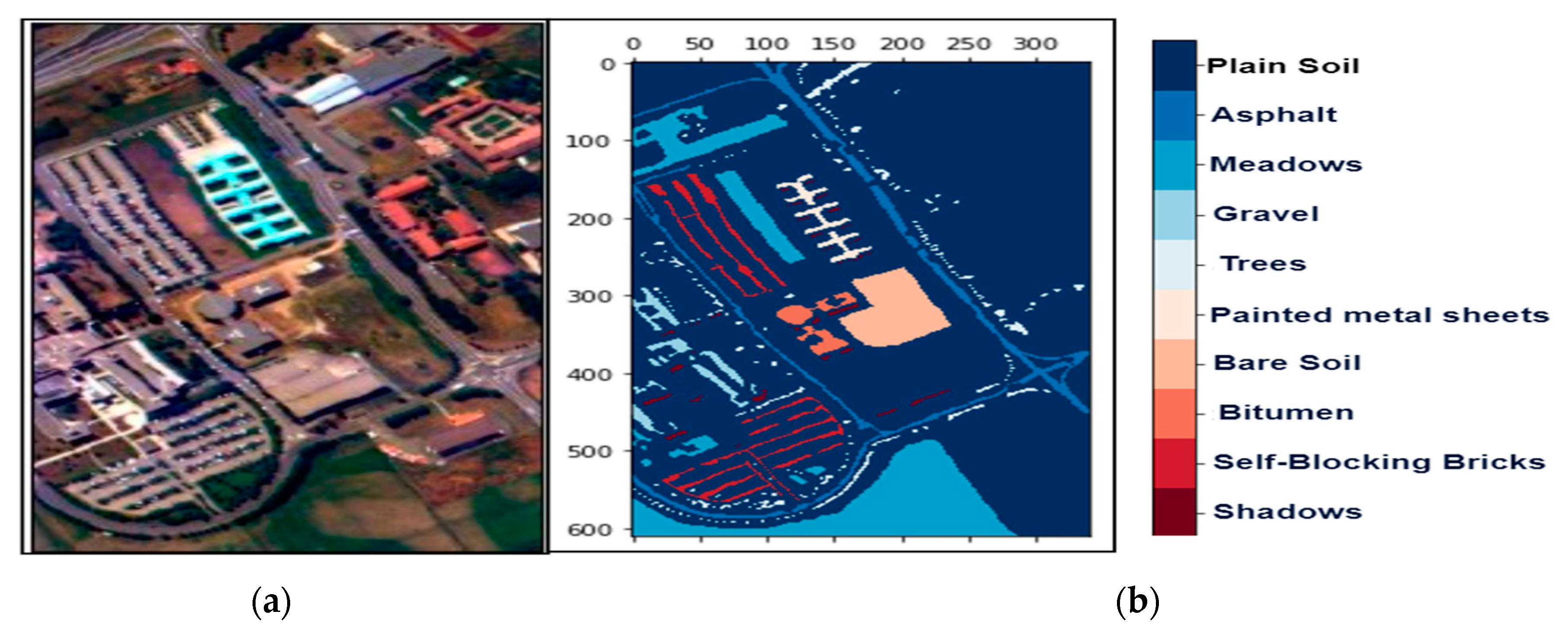
Remotesensing 14 04853 g003
Figure 4. The hyperspectral datasets: Pavia University (PU): (a) The color composite image, (b) the false-color image.
Remotesensing 14 04853 g004
Figure 5. The preprocessing and spectral feature extraction unit for HSI.
Remotesensing 14 04853 g005
Figure 6. The feature extraction unit for the subsampled multi-grained scanning: subsampling schema for sliding window or granularity size (a) 9 × 9, (b) 18 × 18, (c) 27 × 27.
Remotesensing 14 04853 g006aRemotesensing 14 04853 g006b
Figure 7. The classification unit for HSI: The schematic structure for the enhanced deep CF.
Remotesensing 14 04853 g007
Figure 8. The comparison of precision, recall, F_Score, kappa score, and overall accuracy achieved by our proposed model ADA-Es-gcForest for different principal components for (a) IP dataset, (b) SV dataset, (c) PU dataset.
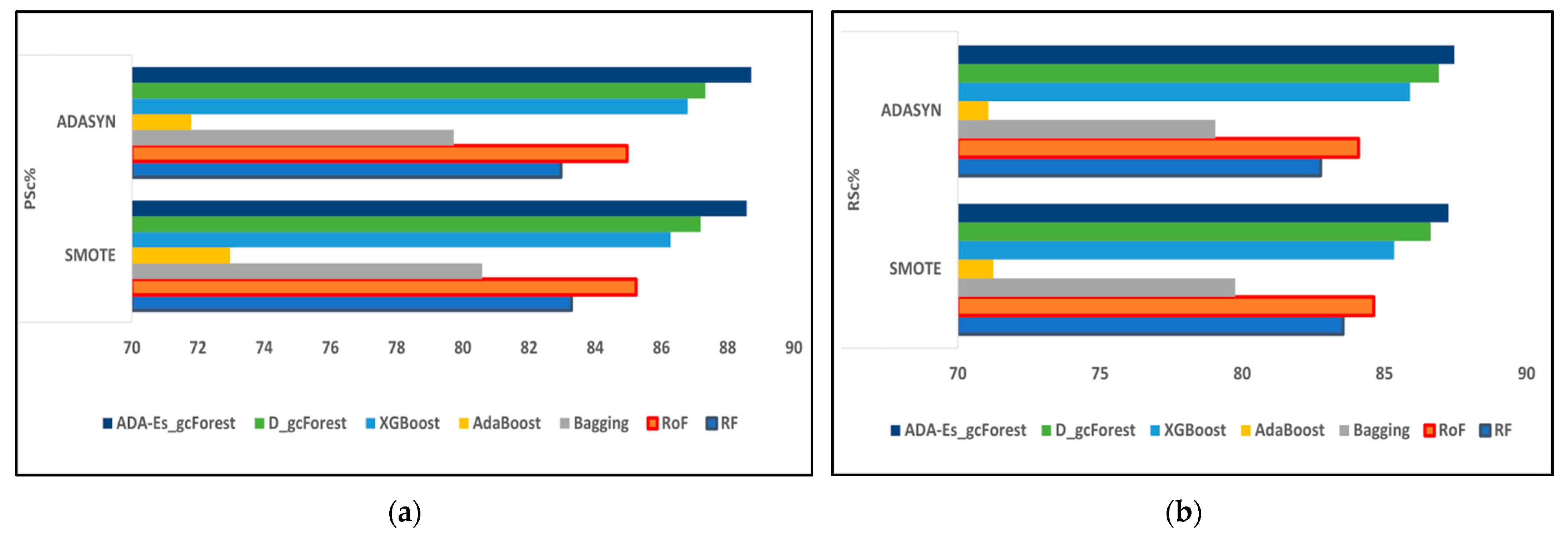
Remotesensing 14 04853 g008
Figure 9. The comparison of assessment metrics between the classifier models RF, RoF, bagging, AdaBoost, XGBoost, DgcForest, and our proposed model ADA-Es-gcForest for 40% IP test sets: (a) PSc%, (b) RSc%, (c) FSc%, and (d) KSc%.
Remotesensing 14 04853 g009aRemotesensing 14 04853 g009b
Figure 10. The comparison of assessment metrics between the classifier models RF, RoF, bagging, AdaBoost, XGBoost, DgcForest, and our proposed model ADA-Es-gcForest for 40% SV test sets: (a) PSc%, (b) RSc%, (c) FSc%, and (d) KSc%.
Remotesensing 14 04853 g010
Figure 11. The comparison of assessment metrics between the classifier models RF, RoF, bagging, AdaBoost, XGBoost, DgcForest, and our proposed model ADA-Es-gcForest for 40% PU test sets: (a) PSc%, (b) RSc%, (c) FSc%, and (d) KSc%.
Remotesensing 14 04853 g011
Figure 12. The classification maps obtained by our proposed model ADA-Es-gcForest for the HSI datasets: (a) IP, (b) SV, and (c) PU.
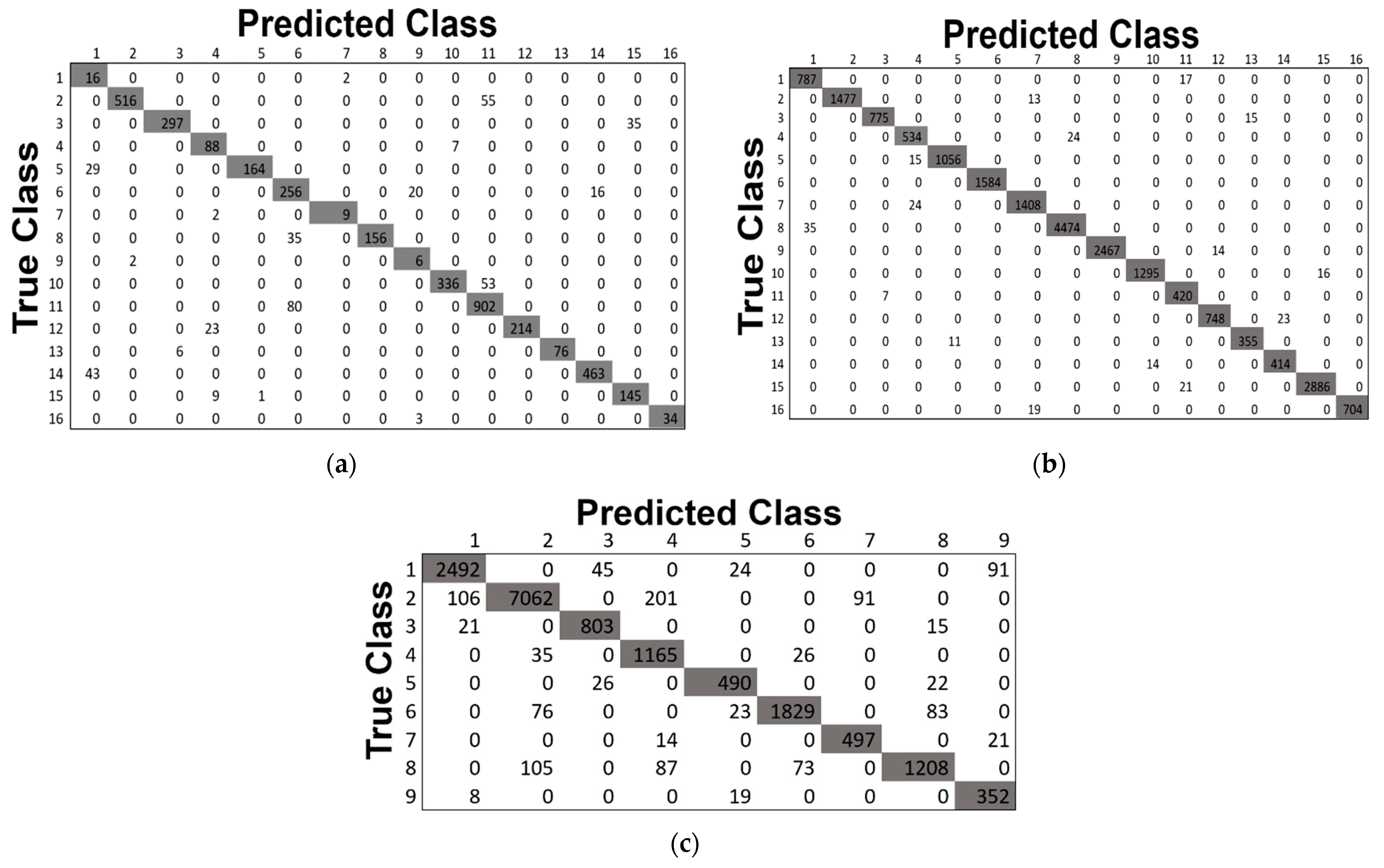
Remotesensing 14 04853 g012
Figure 13. The confusion matrices obtained by our proposed model ADA-Es-gcForest for the HSI datasets: (a) IP, (b) SV, and (c) PU.
Remotesensing 14 04853 g013
Table 1. The ground truth for the HSI datasets: IP, SV, and PU.
The DatasetIndian PinesSalinas Valley
Class No.Class NameOriginalTrainTestClass NameOriginalTrainTest
1Alfalfa462818Brocoli_green_weeds_120091205804
2Corn-notill1428857571Brocoli_green_weeds_2372622361490
3Corn-mintill830498332Fallow19761186790
4Corn23714295Fallow_rough_plow1394836558
5Grass-pasture483290193Fallow_smooth267816071071
6Corn-trees730438292Stubble395923751584
7Corn-pasture-mowed281711Celery357921471432
8Hay-windrowed478287191Grapes_untrained1127167624509
9Oats20128Soil_vinyard_develop620337222481
10Soybeans-notill972583389Corn_senesced_green_weeds327819671311
11Soybeans-mintill24551473982Lettuce_romaine_4wk1068641427
12Soybeans-clean593356237Lettuce_romaine_5wk19271156771
13Wheat20512382Lettuce_romaine_6wk916550366
14Woods1265759506Lettuce_romaine_7wk1070642428
15Buildings-Grass-Trees-Drivers386231155Vinyard_untrained726843612907
16Stone-steel-Towers935637Vinyard_vertical_trellis18071084723
Total 10,24961504099 54,12932,47721,652
The DatasetPavia University
Class No.Class NameOriginalTrainTest
1Asphalt663139792652
2Meadows18,64911,1897460
3Gravel20991260839
4Trees306418381226
5Painted metal sheets1345807538
6Bare Soil502930182011
7Bitumen1330798532
8Self-Blocking Bricks368222091473
9Shadows947568379
Total 42,77625,66617,110
Table 2. Complete hardware/software specification information.
Item NameSpecification
ProcessorIntel® Core™ i7-11800H (2.3 GHz)
RAM16GB DDR4 3200MHz
GPU4GB NVIDIA GeForce RTX 3050 Ti
OSWindows 11
Python Version3.9
Python PackagesTensorflow, Keras, Scikit etc. (latest versions)
Table 3. The hyperparameter configuration of PCA.
Hyperparameter Configured Value
Number of components20, 40, 50, 60 (for comparison)
WhitenTrue (ensures uncorrelated products with unit component-wise variances for the input samples)
Svd_solverAuto (default but can be adaptive depending on the input sample size and number of components)
Table 4. The hyperparameter configuration of SMOTE and ADASYN.
Hyperparameter Configured Value
Sampling strategyMinority (we have mostly chosen the minor classes to create a similar number of samples as the major classes)
k-NN5 (count of NNs used to generate synthetic samples)
Table 5. The hyperparameter configuration and feature generation of subsampled multi-grained scanning.
Subsampling Schema Sl No. (i)Granularity Size (mi)Stride Step-Size (si)Sampling Rate (r)Number of Feature Instances (I)Subsampled Instance Count (II′)New Feature Vector Dimension (di)
1910.5 ( M + N 16 2 ) 2 ( M + N 16 ) 2 8 2 D × ( M + N 16 ) 2 8
21810.5 ( M + N 34 2 ) 2 ( M + N 34 ) 2 8 2 D × ( M + N 34 ) 2 8
32710.5 ( M + N 52 2 ) 2 ( M + N 52 ) 2 8 2 D × ( M + N 52 ) 2 8
Table 6. The hyperparameter configuration of improved deep cascade forest.
HyperparameterConfigured Value
Number of Forests4 (two RFs and two CRFs)
Number of DTs in RF500
Number of DTs in CRF1000
Table 7. The summarization of the variation of cascade layer count with the number of PCA components for the HSI datasets.
n-PCA IPSVPU
20222
40233
50334
60344
Table 8. The result in terms of classification accuracies (%) for the IP dataset obtained by the ensemble classifiers: RF, RoF, bagging, AdaBoost, XGBoost, DgcForest, and our proposed ADA-Es-gcForest along with their combination with the oversampling technique SMOTE with the class imbalance ratio 73.6 and 40% of testing samples.
T-40%
Classifier
RFRoFBaggingAdaBoostXGBoostDgcForestADA-Es-gcForest
OversamplerSMOTEADASYNSMOTEADASYNSMOTEADASYNSMOTEADASYNSMOTEADASYNSMOTEADASYNSMOTEADASYN
OA%80.07 ± 0.6379.88 ± 1.0585.01 ± 1.6784.47 ± 1.0375.82 ± 1.5373.92 ± 0.9968.66 ± 1.4366.04 ± 1.7485.11 ± 1.381.5 ± 1.0285.08 ± 1.5987.01 ± 1.6285.58 ± 0.7689.7 ± 1.24
AA%83.63 ± 0.7581.62 ± 0.6886.29 ± 1.0386.06 ± 0.9678.65 ± 1.6877.62 ± 1.5674.72 ± 0.6572.07 ± 1.3786.9 ± 1.583.56 ± 0.7985.19 ± 1.2288.95 ± 1.1986.15 ± 0.5591.47 ± 0.98
171.26 ± 0.7574.55 ± 0.5770.25 ± 0.8865.66 ± 1.1370.72 ± 1.2481.66 ± 1.5782.18 ± 1.5274.98 ± 1.4285.1 ± 1.5876.03 ± 0.9480.57 ± 1.3784.46 ± 1.6989.77 ± 1.590.5 ± 1.01
281.65 ± 0.6864.24 ± 1.3487.55 ± 0.6268.52 ± 0.5787.62 ± 0.6369.43 ± 0.7283.92 ± 1.7174.92 ± 1.5582.1 ± 1.0871.19 ± 1.6169.87 ± 1.1873.78 ± 1.3689.56 ± 1.7292.64 ± 0.68
372.43 ± 0.5887.75 ± 0.5566.33 ± 0.5268.73 ± 0.5877.87 ± 1.2373.53 ± 1.6275.84 ± 1.267.82 ± 0.6662.86 ± 1.0366.55 ± 1.6985.09 ± 1.489 ± 1.3687.42 ± 1.1488.78 ± 1.35
464.72 ± 0.7185.25 ± 1.7980.82 ± 1.3279.84 ± 1.1966.06 ± 1.271.95 ± 1.6777.92 ± 164.04 ± 1.380.27 ± 1.1982.42 ± 0.7179.73 ± 1.0783.46 ± 1.2588.81 ± 1.189.56 ± 0.67
564.98 ± 1.7883.03 ± 1.6768.41 ± 1.7674.45 ± 0.681.63 ± 1.6180.73 ± 0.9167.78 ± 0.5885.12 ± 0.786.86 ± 1.6376.63 ± 1.2677.22 ± 0.5467.12 ± 1.0387.46 ± 1.3790.26 ± 1.2
677.02 ± 0.7282.8 ± 0.5370.12 ± 0.7686.92 ± 1.872.85 ± 0.5781.62 ± 1.780.11 ± 0.9869.48 ± 0.7365.82 ± 0.8572.22 ± 1.6763.79 ± 0.6482.76 ± 1.7186.2 ± 1.7389.33 ± 0.97
769.33 ± 0.8584.12 ± 0.5371.79 ± 0.8173.08 ± 1.2177.91 ± 0.6769.85 ± 1.5271.01 ± 1.2779.17 ± 0.9767.48 ± 0.8387.21 ± 0.5379.66 ± 1.7184.91 ± 1.3289.45 ± 1.4689.5 ± 1.57
888.72 ± 1.3265.26 ± 0.668.41 ± 1.7884.55 ± 0.9288.71 ± 1.7881.8 ± 1.1663.78 ± 0.8778.78 ± 0.9778.91 ± 1.7963.2 ± 1.6583.15 ± 1.1570.19 ± 0.6888.7 ± 1.0891.6 ± 1.17
963.1 ± 1.0176.66 ± 0.8262.43 ± 1.784.71 ± 0.5285.56 ± 0.5565.64 ± 0.9776.41 ± 1.3676.04 ± 1.0568.31 ± 1.0462.56 ± 1.2186.37 ± 1.3774.88 ± 0.5386.69 ± 0.5191.36 ± 1.12
1076.21 ± 1.4486.38 ± 0.5768.62 ± 1.0668.14 ± 1.2765.16 ± 1.4988.1 ± 1.879.88 ± 1.2188.47 ± 0.5773.28 ± 1.2374.23 ± 1.1288.36 ± 0.7964.37 ± 1.1587.46 ± 0.6791.06 ± 0.56
1164.53 ± 0.8563 ± 1.6862.4 ± 1.5668.13 ± 1.1787.24 ± 1.0365.79 ± 1.7775.17 ± 1.5770.01 ± 1.4162.45 ± 1.7764.88 ± 1.183.34 ± 1.578.46 ± 1.5588.4 ± 0.8789.16 ± 1.1
1280.71 ± 0.686.88 ± 1.6275.41 ± 1.3165.04 ± 0.6286.28 ± 1.5274.26 ± 1.1780.34 ± 1.5662.66 ± 0.9587.03 ± 1.568.39 ± 0.7477.66 ± 1.5377.08 ± 0.5486.94 ± 1.0390.49 ± 1.28
1379.3 ± 1.4271.59 ± 1.7977.38 ± 0.872.43 ± 1.0182.15 ± 0.5271.77 ± 0.7361.27 ± 1.3875.52 ± 0.7673.33 ± 1.6683.98 ± 1.4162.41 ± 1.3788.16 ± 0.9190 ± 1.3491.58 ± 0.62
1474.59 ± 0.7565.43 ± 1.3580.54 ± 1.4984.27 ± 1.6787.08 ± 1.4783.7 ± 1.5388.5 ± 1.2480.88 ± 1.5263.63 ± 1.6464.34 ± 1.0265.81 ± 0.8689.2 ± 1.3288.01 ± 1.7689.18 ± 0.72
1578.09 ± 0.9686.67 ± 1.684.97 ± 0.7574.62 ± 0.7784.68 ± 0.9463.57 ± 1.1579.32 ± 1.2564.94 ± 0.5269.92 ± 1.7489.28 ± 0.6265.49 ± 1.7183.6 ± 1.5286.3 ± 1.7192.7 ± 0.64
1665.89 ± 1.6286.01 ± 1.1870.44 ± 1.1675.5 ± 0.7864.08 ± 0.9383.85 ± 1.3662.78 ± 0.7271.68 ± 1.2564.72 ± 1.7375.98 ± 0.8774.21 ± 1.1588.88 ± 1.389.89 ± 1.3189.29 ± 1.48
Table 9. The result in terms of classification accuracies (%) for the IP dataset obtained by the ensemble classifiers: RF, RoF, bagging, AdaBoost, XGBoost, DgcForest, and our proposed ADA-Es-gcForest along with their combination with the oversampling technique SMOTE with the class imbalance ratio 73.6 and 50% of testing samples.
T-50%
Classifier
RFRoFBaggingAdaBoostXGBoostDgcForestADA-Es-gcForest
OversamplerSMOTEADASYNSMOTEADASYNSMOTEADASYNSMOTEADASYNSMOTEADASYNSMOTEADASYNSMOTEADASYN
OA% 79.74 ± 2.25 75.95 ± 2.27 80.19 ± 1.93 78.27 ± 1.04 72.15 ± 2.32 68.53 ± 2.15 64.79 ± 1.8 62.99 ± 1.68 80.45 ± 0.94 77.46 ± 1.37 81.97 ± 1.6884.39 ± 1.7482.58 ± 1.0987.29 ± 1.72
AA% 81.03 ± 2 80.1 ± 1.05 83.51 ± 2.03 81.35 ± 1.79 76.29 ± 0.99 73.85 ± 2.05 70.98 ± 2.22 69.06 ± 1.9 83.56 ± 0.91 80.34 ± 2.01 83.2 ± 1.0887.73 ± 1.0884.69 ± 1.0989.59 ± 1.48
1 74.71 ± 2.37 64.22 ± 1.26 70.42 ± 2.03 84.62 ± 1.42 86.92 ± 1.26 82.54 ± 1.71 64.8 ± 1.05 88.39 ± 1.58 87.46 ± 1.82 68.98 ± 1.28 80.35 ± 1 74.91 ± 1.12 83.58 ± 0.99 85.55 ± 0.98
2 86.97 ± 1.6 82.37 ± 1.47 75.8 ± 1.64 65.6 ± 0.93 75.86 ± 1.33 74.52 ± 1.22 88.33 ± 1.92 80.76 ± 1.61 71.15 ± 1.51 77.36 ± 1.19 79.71 ± 1.73 81.16 ± 1.83 83.53 ± 1.08 82.71 ± 2.14
3 76.53 ± 1.33 70.77 ± 2.31 76.14 ± 1.3 87.56 ± 1.17 84.02 ± 1.74 88.67 ± 1.59 76.52 ± 0.92 77.67 ± 2.35 86.71 ± 1.31 74.61 ± 1.3 71.51 ± 1.95 78.1 ± 2.23 84.24 ± 1.95 84.93 ± 1.9
4 86.1 ± 1.48 71.91 ± 0.96 72.26 ± 1.85 71.33 ± 1.3 83.21 ± 1.74 70.2 ± 1.8 77.54 ± 1.24 78.83 ± 0.92 72.62 ± 1.39 68.38 ± 1.92 68.37 ± 1.34 84.36 ± 1.13 83.14 ± 1.23 83.55 ± 1.83
5 83.9 ± 1.96 88.92 ± 2.21 84.49 ± 1.11 62.61 ± 2.16 77.58 ± 1.99 73.82 ± 1.99 76.51 ± 1.22 80.67 ± 1.77 72.98 ± 1.67 72.06 ± 1.87 76.03 ± 1.49 78.03 ± 1.21 86.39 ± 2 84.44 ± 2.23
6 75.59 ± 2.1 79.21 ± 1.17 64.48 ± 0.9 61.68 ± 1.18 85.96 ± 1.98 65.71 ± 1.55 68.38 ± 2.34 62.99 ± 2.11 80.17 ± 1.14 72.56 ± 1.99 71.77 ± 1.07 82.28 ± 0.95 83.17 ± 1.12 86.37 ± 1.78
7 74.2 ± 1.86 62.1 ± 2.22 77.08 ± 1.17 65.43 ± 1.17 65.31 ± 1.71 77.58 ± 2.28 64.14 ± 1.5 76.69 ± 1.19 80.88 ± 2.23 84.02 ± 1.69 86.07 ± 1.87 76.12 ± 0.93 85.55 ± 1.11 85.53 ± 2.06
8 70.32 ± 2.05 69.17 ± 2.37 86.12 ± 1.84 72.08 ± 2.21 76.77 ± 1.61 71.27 ± 1.8 80.67 ± 1.42 74.27 ± 1.18 78.03 ± 1.88 77.11 ± 2.11 77.94 ± 1.43 66.11 ± 1.38 82.23 ± 2.36 84.27 ± 0.96
9 68.93 ± 1.03 63.76 ± 1.43 62.81 ± 1.5 79.94 ± 0.96 88.13 ± 2.01 70.58 ± 1.22 74.16 ± 2.21 87.84 ± 2.32 87.58 ± 2.08 87.66 ± 1.62 73.81 ± 1.41 75.4 ± 2 86.55 ± 1.7 86.71 ± 1.81
10 88.21 ± 1.96 76.34 ± 1.8 65.41 ± 1.19 86.21 ± 1.04 69.55 ± 2.35 69.05 ± 0.96 76.63 ± 1.09 75.88 ± 2.36 86.9 ± 1.43 70.13 ± 1.13 69.96 ± 1.52 67.1 ± 2.17 86.18 ± 1.95 85.06 ± 2.13
11 79.9 ± 2.39 86.99 ± 1.19 77.22 ± 1.45 77.92 ± 1.89 82.25 ± 1.1 74.19 ± 1.53 80.14 ± 1.96 66.01 ± 1.77 88.15 ± 1 75.06 ± 1.92 77.31 ± 0.92 75.45 ± 1.81 86.11 ± 2.2 84.99 ± 1.48
12 62.65 ± 2.12 82.49 ± 1.53 84 ± 1.03 83.15 ± 1.35 81.31 ± 1.33 84.19 ± 1.28 67.29 ± 1.02 81.05 ± 1.04 86.52 ± 1.99 86.18 ± 1.78 87.09 ± 1.67 69.5 ± 2.23 84.24 ± 1 86.79 ± 1.32
13 73.09 ± 1.14 69.74 ± 1.31 84.01 ± 1.61 65.27 ± 2.27 71.28 ± 0.97 62.5 ± 2.04 63.35 ± 2.14 66.37 ± 1.88 70.13 ± 1.23 79.98 ± 2.32 79.08 ± 1.55 63.25 ± 0.93 82.53 ± 2.37 85.4 ± 1.65
14 69.6 ± 2.22 70.24 ± 1.25 70.98 ± 2.18 63.22 ± 2.07 72.71 ± 1.94 86.44 ± 1.07 71.81 ± 1.19 76.83 ± 0.96 87.66 ± 1.1 66.86 ± 1.96 66.2 ± 1.58 82.98 ± 2.03 83.35 ± 1.36 83.36 ± 1.89
15 87.68 ± 1.36 62.22 ± 1.92 65.09 ± 1.22 82.1 ± 2.15 75.56 ± 1.25 79.21 ± 1.32 66.99 ± 2.33 77.09 ± 1.68 73.58 ± 1.51 67.82 ± 2.25 67.4 ± 1.32 66.14 ± 1.05 85.27 ± 1.22 82.72 ± 1.54
16 75.59 ± 2.13 71.75 ± 2.29 82.95 ± 1.19 87.04 ± 1.5 67.73 ± 1.65 67.44 ± 1.5 87.93 ± 1.21 71.58 ± 2.24 65.85 ± 1.1 74.13 ± 1.28 79.33 ± 1.11 64.53 ± 1.26 86.66 ± 1.42 82.58 ± 1.74
Table 10. The result in terms of classification accuracies (%) for the IP dataset obtained by the ensemble classifiers: RF, RoF, bagging, AdaBoost, XGBoost, DgcForest, and our proposed ADA-Es-gcForest along with their combination with the oversampling technique SMOTE with the class imbalance ratio 73.6 and 60% of testing samples.
T-60%
Classifier
RFRoFBaggingAdaBoostXGBoostDgcForestADA-Es-gcForest
OversamplerSMOTEADASYNSMOTEADASYNSMOTEADASYNSMOTEADASYNSMOTEADASYNSMOTEADASYNSMOTEADASYN
OA% 76.81 ± 2.59 73.76 ± 2.98 78.68 ± 2.44 77.17 ± 2.77 68.74 ± 2.47 63.26 ± 1.87 63.59 ± 1.76 59.17 ± 2.92 78.95 ± 2.68 74.66 ± 2.82 78.38 ± 2.0182.37 ± 3.0580.58 ± 2.2285.33 ± 2.06
AA% 78.71 ± 3.01 77.24 ± 1.79 80.75 ± 1.9 79.25 ± 1.47 73.38 ± 2.24 67.48 ± 2.02 67.62 ± 1.46 65.82 ± 2.83 81.05 ± 2.96 77.92 ± 1.33 81.89 ± 3.184.76 ± 2.5582.11 ± 2.4787.92 ± 2.72
1 71.17 ± 1.52 70.46 ± 1.4 78.42 ± 2.28 65.58 ± 2.58 61.2 ± 1.24 76.59 ± 2.58 68.71 ± 1.48 67.4 ± 2.96 63.9 ± 2.89 72.28 ± 2.35 71.29 ± 1.61 62.61 ± 3.07 82.36 ± 2.62 79.21 ± 2.74
2 71.62 ± 2.33 72.89 ± 2.13 62.58 ± 2.94 79.83 ± 2.33 78.42 ± 2.83 85.47 ± 2.88 67.6 ± 3 86.88 ± 2.86 66.11 ± 3.1 87.8 ± 2.96 62.69 ± 1.25 77.4 ± 1.78 82.11 ± 1.72 83.25 ± 2.95
3 67.42 ± 2.15 62.09 ± 1.51 64.45 ± 1.8 74.27 ± 1.71 88.92 ± 1.62 66.04 ± 2.46 69.08 ± 2.8 75.71 ± 1.58 61.2 ± 1.45 62.03 ± 2.21 85.93 ± 1.89 86.56 ± 2.87 81.68 ± 1.8 83.73 ± 2.73
4 67.44 ± 1.69 71.74 ± 1.19 67.3 ± 2.34 69.94 ± 2.31 82.67 ± 2.19 84.72 ± 1.59 66.32 ± 3.04 65.29 ± 2.04 67.22 ± 1.57 66.29 ± 2.68 77.16 ± 1.83 82.89 ± 2.2 79.99 ± 1.62 82.58 ± 1.46
5 85.16 ± 1.58 86.92 ± 2.01 79.03 ± 1.4 84.09 ± 2.83 85.38 ± 2.28 80.93 ± 1.54 86.03 ± 1.11 61.11 ± 1.34 66.41 ± 1.33 71.67 ± 2.86 83.7 ± 2.7 81.26 ± 2.89 79.7 ± 1.7 82.69 ± 1.45
6 86.58 ± 2.59 63.31 ± 1.84 81.6 ± 2.52 80.61 ± 1.92 72.19 ± 1.84 64.96 ± 1.66 73.15 ± 1.37 69.2 ± 1.13 82.85 ± 2.37 62.51 ± 1.78 77.41 ± 1.6 79.09 ± 1.42 80.01 ± 2.7 82.71 ± 1.67
7 76.83 ± 1.72 69.37 ± 2.09 69.63 ± 1.3 77.77 ± 1.98 83.43 ± 2.47 87.75 ± 1.98 72.82 ± 2.21 66.7 ± 1.96 71.59 ± 2.24 84.11 ± 2.2 77.17 ± 2.66 66.65 ± 2.48 81.61 ± 2.59 79.7 ± 1.49
8 81.56 ± 1.38 78.81 ± 1.16 61.04 ± 1.73 87.76 ± 2.6 79.07 ± 1.4 73.25 ± 2.95 77.61 ± 2.24 85.89 ± 3.06 67.41 ± 2.29 74.44 ± 1.29 86.55 ± 2.66 88.47 ± 1.26 83.29 ± 2.77 82.58 ± 2.75
9 77.72 ± 2.59 88.21 ± 1.15 80.3 ± 1.28 76.84 ± 2.38 83.78 ± 1.71 78.7 ± 2.95 78.9 ± 2.05 88.86 ± 2.79 67.89 ± 1.33 71.24 ± 2.64 62.19 ± 1.35 68.72 ± 2.12 79.68 ± 1.5 81.78 ± 2.94
10 67.64 ± 1.18 75.85 ± 2.66 88.78 ± 1.69 78.36 ± 1.99 70.41 ± 1.63 85.29 ± 2.54 86.89 ± 1.6 78.74 ± 1.83 87.63 ± 1.82 62.44 ± 1.29 72.83 ± 2.05 70.6 ± 2.25 83.97 ± 1.3 79.31 ± 2.1
11 72.85 ± 2.66 83.22 ± 1.47 65.45 ± 1.44 66.8 ± 2.94 66.15 ± 2.23 76.91 ± 1.3 71.41 ± 1.63 69.9 ± 3.01 80.45 ± 3.03 72.34 ± 1.48 82.44 ± 2.78 77.53 ± 1.53 82.39 ± 2.2 83.96 ± 2.39
12 75.12 ± 2.75 85.56 ± 2.79 70.5 ± 2.6 73.84 ± 1.56 63.55 ± 1.8 86.09 ± 1.18 63.2 ± 1.18 63.16 ± 2.22 84.2 ± 2.58 83.63 ± 2.15 64.76 ± 3.05 76.98 ± 1.41 81.69 ± 2.75 84.57 ± 2.22
13 64.68 ± 1.63 64.72 ± 2.37 79.93 ± 3.02 70.09 ± 2.42 88.97 ± 2.56 62.42 ± 2.86 78.91 ± 1.16 75.27 ± 1.84 74.51 ± 2.7 74.01 ± 3.07 68.06 ± 2.55 65.6 ± 3.07 82.84 ± 2.12 80.81 ± 1.67
14 63.26 ± 1.8 84.97 ± 2.11 65.47 ± 2.9 69.24 ± 1.6 86.22 ± 2.65 87.11 ± 2.88 78.82 ± 2.51 88.2 ± 1.32 85.59 ± 2.96 77.25 ± 3.03 88.23 ± 1.69 74.58 ± 1.49 83.7 ± 2.88 84.81 ± 2.54
15 86.53 ± 1.19 83.63 ± 2.55 67.97 ± 1.16 81.72 ± 2.44 66.65 ± 1.48 62.21 ± 1.37 77.64 ± 2.11 81.76 ± 1.72 84.22 ± 1.4 86.2 ± 3.05 69.53 ± 2.98 70.19 ± 2.39 82.95 ± 1.84 80.09 ± 1.57
16 70.17 ± 1.95 80.89 ± 2.11 83.93 ± 2.79 78.88 ± 2.48 72.92 ± 2.78 88.67 ± 2.42 76.96 ± 1.76 65.7 ± 3.03 76.01 ± 2.73 83.22 ± 1.49 80.75 ± 1.63 61.47 ± 2.18 81.15 ± 1.56 81.65 ± 1.79
Table 11. The result in terms of classification accuracies (%) for the SV dataset obtained by the ensemble classifiers: RF, RoF, bagging, AdaBoost, XGBoost, DgcForest, and our proposed ADA-Es-gcForest along with their combination with the oversampling technique SMOTE with the class imbalance ratio 12.51 and 40% of testing samples.
T-40%
Classifier
RFRoFBaggingAdaBoostXGBoostDgcForestADA-Es-gcForest
OversamplerSMOTEADASYNSMOTEADASYNSMOTEADASYNSMOTEADASYNSMOTEADASYNSMOTEADASYNSMOTEADASYN
OA% 90.3 ± 1.4 89.58 ± 0.77 93.41 ± 0.68 90.92 ± 1.17 86.76 ± 0.66 86.14 ± 1.42 78.77 ± 0.6 78.43 ± 0.7 89.61 ± 1.79 89.29 ± 1.08 92.35 ± 1.7195.02 ± 0.7795.58 ± 0.9797.54 ± 0.86
AA% 92.74 ± 1.14 90.9 ± 0.51 94.58 ± 0.58 93.69 ± 1.49 88.22 ± 0.52 87.58 ± 1.28 80.3 ± 0.55 79.64 ± 0.91 93.72 ± 1.07 93.29 ± 1.2 94.43 ± 0.6896.49 ± 1.0297.04 ± 1.7598.76 ± 1.26
1 75.02 ± 0.6 85.34 ± 0.63 70 ± 0.86 70.76 ± 1.23 78.58 ± 0.75 77.47 ± 0.82 83.71 ± 1.64 82.91 ± 0.88 83.44 ± 1.27 85.34 ± 0.67 81.79 ± 1.64 81.84 ± 1.28 86.62 ± 0.85 89.03 ± 1.16
2 87.64 ± 0.9 81.21 ± 0.8 87.84 ± 1.36 79.67 ± 1.24 88.59 ± 1.42 76.48 ± 1.06 74.88 ± 1.48 89.33 ± 1.62 75.73 ± 0.75 86.71 ± 0.75 89.44 ± 1.4 84.93 ± 1.23 89.92 ± 1.16 85.21 ± 0.6
3 86.61 ± 1.07 61.58 ± 0.53 73.73 ± 1.79 78.22 ± 0.85 77.33 ± 0.89 74.54 ± 0.61 74.74 ± 1.69 73.55 ± 1.67 64.18 ± 1.55 66.93 ± 1.15 84.78 ± 0.88 91.84 ± 1.05 81.71 ± 1.31 93.84 ± 0.99
4 85.15 ± 1.21 74.86 ± 1.06 77.1 ± 0.81 72.85 ± 0.97 80.7 ± 1.79 72.91 ± 0.97 78.88 ± 1.46 69.18 ± 1.32 64.54 ± 1.06 68.03 ± 0.61 80.38 ± 1.05 89.28 ± 1.42 91.28 ± 1.14 90.72 ± 1.47
5 88.68 ± 0.64 78.32 ± 1.45 71.14 ± 0.78 86.85 ± 1.09 76.16 ± 1.3 75.6 ± 1.27 81.52 ± 1.1 71.46 ± 0.62 70.42 ± 1.5 77.97 ± 0.91 93.61 ± 1.6 96.42 ± 0.53 80.29 ± 0.86 97.28 ± 0.91
6 67.76 ± 0.68 85.73 ± 1.7 67.63 ± 0.64 66.76 ± 1.3 67.79 ± 1.26 82.71 ± 1.61 72.97 ± 0.56 61.6 ± 1.13 65.71 ± 1.28 78.18 ± 0.96 81.44 ± 0.57 81.9 ± 1.64 83.53 ± 1.65 91.62 ± 0.58
7 70.52 ± 0.64 87.88 ± 0.96 87.19 ± 1.06 87.35 ± 1.44 70.12 ± 1.51 71.26 ± 1.2 65.63 ± 0.67 69.4 ± 1.73 77.13 ± 1.41 63.05 ± 1.09 84.65 ± 1.77 95.68 ± 0.95 93.29 ± 1.64 97.99 ± 1.4
8 72.33 ± 1.51 81.82 ± 1.57 65.33 ± 1.18 68.23 ± 1.36 80.9 ± 0.84 81.85 ± 1.79 77.69 ± 0.97 74.91 ± 0.65 88.73 ± 1.26 62.85 ± 1.27 92.07 ± 0.61 94.41 ± 1.41 92.83 ± 1.28 95.1 ± 0.58
9 70.05 ± 1.65 81.16 ± 1.17 67.91 ± 1.23 64.45 ± 0.75 66.12 ± 1.31 86.87 ± 0.54 79.01 ± 1.44 79.3 ± 1.52 73.58 ± 1.48 61.35 ± 1.33 82.73 ± 0.62 95.23 ± 1.05 83.79 ± 1.03 91.94 ± 0.75
10 67 ± 0.76 68.4 ± 1.48 73.74 ± 0.82 76.29 ± 1.61 64.91 ± 1.35 71.54 ± 1.59 80.38 ± 0.71 72.54 ± 1.44 67.7 ± 0.65 69.05 ± 0.68 81.22 ± 1.13 87.14 ± 0.55 89.19 ± 1.13 96.98 ± 1.02
11 85.2 ± 1.32 70.24 ± 1.14 87.28 ± 0.66 70.45 ± 0.55 83.1 ± 1.58 73.6 ± 1.52 75.98 ± 0.68 69.98 ± 0.9 69.31 ± 1.09 67.29 ± 1.07 87.4 ± 1.24 84.85 ± 0.98 87.16 ± 1.42 97.69 ± 0.71
12 70.52 ± 1 70.1 ± 1.15 88.87 ± 1.01 76.04 ± 1.72 67.41 ± 1.15 79.92 ± 0.65 86.39 ± 0.83 64.11 ± 0.7 68.31 ± 1.65 73.93 ± 1.2 80.99 ± 1.43 88.93 ± 1.76 86.88 ± 1.74 93.81 ± 1.55
13 74.11 ± 1.28 62.79 ± 1.22 73.3 ± 1.78 77.29 ± 1.55 87.38 ± 0.87 84.37 ± 1.06 75.51 ± 0.89 68.84 ± 0.69 61.35 ± 1.45 82.06 ± 1.42 83.12 ± 1.76 92.71 ± 1.52 91.79 ± 0.97 93.32 ± 1.19
14 84.85 ± 0.83 85.54 ± 0.5 72.83 ± 1.31 82.14 ± 1.08 80.2 ± 1.72 78.27 ± 1.02 71.27 ± 0.5 71.72 ± 0.75 83.75 ± 1.47 70.86 ± 0.9 83.79 ± 1.42 94.58 ± 1.23 85.15 ± 1.5 90.99 ± 1.64
15 64.09 ± 1.68 71.61 ± 1.15 71.44 ± 1.76 65.77 ± 0.95 85.54 ± 0.83 74.95 ± 1.37 68.82 ± 0.59 67.76 ± 0.68 61.78 ± 0.88 85.55 ± 1.33 84.83 ± 0.58 91.29 ± 1.59 83.53 ± 1.14 81.69 ± 0.61
16 83.6 ± 1.56 76.39 ± 1.43 67.03 ± 1.17 86.53 ± 0.74 70.31 ± 1.08 66.31 ± 1.26 69.77 ± 0.56 78.1 ± 0.97 66.85 ± 1.45 76.16 ± 1.56 87.07 ± 1.7 85.13 ± 1.43 87.8 ± 1.17 86.68 ± 1.04
Table 12. The result in terms of classification accuracies (%) for the SV dataset obtained by the ensemble classifiers: RF, RoF, bagging, AdaBoost, XGBoost, DgcForest, and our proposed ADA-Es-gcForest along with their combination with the oversampling technique SMOTE with the class imbalance ratio 12.51 and 50% of testing samples.
T-50%
Classifier
RFRoFBaggingAdaBoostXGBoostDgcForestADA-Es-gcForest
OversamplerSMOTEADASYNSMOTEADASYNSMOTEADASYNSMOTEADASYNSMOTEADASYNSMOTEADASYNSMOTEADASYN
OA% 86.79 ± 0.99 85.73 ± 1.52 90.89 ± 1.07 88.54 ± 1.04 83.66 ± 1.85 82.93 ± 2.22 75.2 ± 2.03 74.28 ± 1.62 87.16 ± 2.39 85.49 ± 1.12 92.28 ± 1.2193.99 ± 1.4792.58 ± 2.0595.37 ± 1.34
AA% 88.51 ± 1.75 87.59 ± 1.6 92.01 ± 2.12 90.54 ± 1.05 86.91 ± 0.97 85.55 ± 2.32 78.59 ± 2.13 77.76 ± 1.06 89.8 ± 1.38 88.22 ± 1.31 93.52 ± 1.1195.35 ± 2.3994.69 ± 1.896.79 ± 2.09
1 71.91 ± 1.55 63.76 ± 1.6 77.07 ± 0.93 88.48 ± 2.29 81.56 ± 1.98 86.11 ± 1.08 79.51 ± 2.24 70.91 ± 1.3 62.48 ± 1.6 63.33 ± 1.45 91.68 ± 1.09 80.98 ± 1.98 80.99 ± 1.95 80.63 ± 1.53
2 62.02 ± 1.86 78.12 ± 1.7 85.19 ± 1.11 79.83 ± 1.58 64.73 ± 1.35 80.98 ± 0.95 73.34 ± 0.9 86.2 ± 1.44 88.72 ± 1.73 62.35 ± 1.56 87.39 ± 2.35 89.48 ± 1.7 85.22 ± 1.28 86.43 ± 1.44
3 75.66 ± 1 86.2 ± 2 80.87 ± 1.3 73.85 ± 2.22 61.67 ± 2.33 67.04 ± 1.68 66.21 ± 1.18 67.01 ± 1.03 64.04 ± 1.21 87.93 ± 1.57 85.12 ± 0.91 81.56 ± 2.35 91.82 ± 2.37 82.26 ± 2.05
4 87.71 ± 2.05 71.04 ± 1.86 81.03 ± 1.02 70.89 ± 1.59 82.15 ± 1.22 63.83 ± 2.13 73.08 ± 1.7 84.11 ± 1.87 74.83 ± 1.74 83.15 ± 1.41 84.32 ± 1.86 80.27 ± 1.95 80.17 ± 2.16 87.49 ± 1.97
5 86.67 ± 0.96 73.03 ± 1.52 67.9 ± 1.52 71.99 ± 1.2 66.32 ± 1.74 68.28 ± 1.83 77.12 ± 1.28 67.59 ± 1.72 85.95 ± 1.75 87.15 ± 1.77 91.93 ± 1.42 84.01 ± 2.2 81.37 ± 1.59 80.06 ± 2.05
6 88.62 ± 1.06 74.42 ± 2.25 62.4 ± 1.75 75.62 ± 2.13 72.88 ± 1.44 84.87 ± 2.31 72.34 ± 1.75 81.49 ± 2.07 83.57 ± 2.03 85.39 ± 2.37 90.41 ± 1.07 91.3 ± 1.65 89.31 ± 1.23 89.02 ± 1.81
7 77.62 ± 1.33 61.76 ± 1.42 62.36 ± 1.44 77.76 ± 1.7 79.6 ± 1.72 79.17 ± 1.19 71.9 ± 2.17 72.48 ± 1.26 64.81 ± 1.87 82.25 ± 1.74 81.16 ± 2.21 86.8 ± 2.21 87.84 ± 2.01 92.56 ± 1.3
8 62.56 ± 2.14 76.78 ± 1.94 71.59 ± 2.15 82.35 ± 1.54 70.98 ± 0.93 75.06 ± 2.38 81.48 ± 1.44 69.2 ± 1.16 68.72 ± 1.99 61.99 ± 1.01 87.31 ± 1.3 82.58 ± 2.35 89.49 ± 1.11 92.74 ± 1.38
9 64.8 ± 2.04 61.09 ± 1.03 70.5 ± 2.18 78.52 ± 1.55 82.18 ± 2.14 84.9 ± 2.24 64.62 ± 1.45 85.58 ± 2.09 86.42 ± 1.27 83.72 ± 1 88.44 ± 1.23 84.61 ± 1.41 83.82 ± 1.8 85.34 ± 2.02
10 82.52 ± 1.16 61.82 ± 1.67 72.71 ± 2.29 88.64 ± 1.37 82.8 ± 2.24 65.52 ± 1.02 88.26 ± 1.85 66.77 ± 1.65 82.45 ± 1.97 65.49 ± 1.63 88.25 ± 1.94 86.64 ± 1.62 83.76 ± 1.93 87.9 ± 0.95
11 65.8 ± 2.3 61.67 ± 2.27 79.94 ± 1.49 71.12 ± 1.83 65.18 ± 2 68.92 ± 1.97 66.61 ± 2.06 80.3 ± 2.17 82.41 ± 2.01 88.38 ± 1.88 85.41 ± 0.95 81.46 ± 1.19 83.95 ± 1.69 81.06 ± 1.47
12 67.87 ± 1.97 69.98 ± 1.36 68.66 ± 1.66 73.34 ± 1.88 72.03 ± 1.57 80.06 ± 1.75 79.57 ± 1.98 87.48 ± 1.19 74.44 ± 1.92 84.07 ± 1.77 89.66 ± 1.59 83.93 ± 2.35 83.87 ± 2.13 80.78 ± 1.75
13 61.25 ± 1.26 78.21 ± 0.99 65.1 ± 2.08 72.82 ± 1.02 79.36 ± 1.11 71.14 ± 1.26 79.91 ± 1.69 70.17 ± 2.26 66.09 ± 1.9 84.05 ± 1.91 85.2 ± 1.65 91.68 ± 1.68 87.82 ± 1.38 81.51 ± 1.41
14 62.68 ± 1.51 65.42 ± 2.04 65.08 ± 1.48 69.37 ± 1.95 69.76 ± 1.88 77.39 ± 2.09 74.13 ± 1.56 69.25 ± 1.59 71.17 ± 1.31 84.27 ± 1.97 90.32 ± 1.6 85.68 ± 2.1 90.65 ± 2.04 83.92 ± 1.47
15 79.56 ± 1.1 78.49 ± 1.97 78.63 ± 0.95 69.13 ± 1.68 64.24 ± 2.34 66.49 ± 1.14 66.75 ± 1.7 69.43 ± 2.23 65.77 ± 1.11 73.53 ± 2.31 86.28 ± 1.66 90.65 ± 1.1 87.21 ± 0.96 92.84 ± 1.18
Table 13. The result in terms of classification accuracies (%) for the SV dataset obtained by the ensemble classifiers: RF, RoF, bagging, AdaBoost, XGBoost, DgcForest, and our proposed ADA-Es-gcForest along with their combination with the oversampling technique SMOTE with the class imbalance ratio 12.51 and 60% of testing samples.
T-60%
Classifier
RFRoFBaggingAdaBoostXGBoostDgcForestADA-Es-gcForest
OversamplerSMOTEADASYNSMOTEADASYNSMOTEADASYNSMOTEADASYNSMOTEADASYNSMOTEADASYNSMOTEADASYN
OA% 83.92 ± 2.03 83.71 ± 2.88 90.65 ± 3.02 87.78 ± 1.32 84.79 ± 1.28 80.93 ± 1.78 71.38 ± 2.14 67.77 ± 2.1 84.36 ± 3.03 83.54 ± 2.28 90.06 ± 1.3291.93 ± 1.991.58 ± 1.793.18 ± 2.34
AA% 85.71 ± 1.44 85.08 ± 2.82 91.27 ± 2.33 89.69 ± 1.43 86.29 ± 2.07 84.28 ± 1.7 75.41 ± 1.88 72.92 ± 2.32 86.01 ± 1.79 85.39 ± 1.55 91.22 ± 1.8293.04 ± 1.4192.69 ± 1.6394.89 ± 2.53
1 64.6 ± 1.51 87.76 ± 1.42 78.3 ± 1.28 85.32 ± 1.98 88.27 ± 1.57 85.58 ± 2.4 72.6 ± 1.93 75.29 ± 1.7 77.89 ± 2.23 68.14 ± 2.98 80.05 ± 2.78 83.22 ± 1.25 88.24 ± 2.62 86.11 ± 1.21
2 81.54 ± 2.85 65.17 ± 2.31 66.76 ± 2.86 88.49 ± 1.85 77.57 ± 1.55 65.67 ± 1.21 75.26 ± 1.19 71.55 ± 2.7 67.81 ± 2.09 72.98 ± 2.46 81.82 ± 1.19 79.21 ± 2.53 82.8 ± 1.23 78.72 ± 2.27
3 80.47 ± 1.32 67.05 ± 1.3 81.15 ± 1.47 81.44 ± 2.95 79.43 ± 2.15 75.32 ± 3.07 72.4 ± 2.01 81.29 ± 2.19 74.44 ± 2.7 63.41 ± 2.37 77.24 ± 1.81 76.19 ± 1.69 83.88 ± 1.42 80.79 ± 1.27
4 80.96 ± 2.37 78.11 ± 2.65 81.4 ± 2.16 63.28 ± 1.16 82.57 ± 1.98 88 ± 1.68 61.05 ± 3.02 68.18 ± 2.29 63.21 ± 2.43 63.93 ± 1.34 85.23 ± 1.82 77.93 ± 1.41 85.83 ± 1.21 80.47 ± 1.49
5 83.57 ± 2.85 79.63 ± 1.41 70.4 ± 2.23 67.27 ± 1.3 63.95 ± 3.08 81.24 ± 2.62 87.43 ± 1.57 63.82 ± 2.08 79.1 ± 2.83 79.64 ± 2.09 83.58 ± 2.74 76.6 ± 1.3 86.96 ± 2 88.1 ± 3.08
6 70.27 ± 2.94 79.36 ± 1.16 64.24 ± 2.79 82.09 ± 1.67 62.85 ± 1.38 70.72 ± 1.72 84.11 ± 2.45 64.37 ± 2.66 81.74 ± 1.25 63.9 ± 2.67 76.33 ± 1.34 77.59 ± 2.2 81.97 ± 2.06 83.77 ± 2.84
7 72.58 ± 2.98 61.26 ± 1.55 78.45 ± 2.92 69.65 ± 2.33 68.86 ± 2.55 78.14 ± 2.24 84.8 ± 1.23 87 ± 2.03 63.4 ± 3.08 85.05 ± 1.33 75.24 ± 1.94 86.87 ± 3.03 79.4 ± 2.3 83.64 ± 2.59
8 80.74 ± 3.1 68.5 ± 1.58 86.07 ± 1.86 87.92 ± 2.4 62.62 ± 2.13 78.17 ± 2.95 75.23 ± 2.25 87.34 ± 2.85 85.72 ± 2.43 84.71 ± 1.36 86.65 ± 2.55 87.19 ± 1.32 82.14 ± 1.86 83.76 ± 1.44
9 84.77 ± 1.69 68.26 ± 2.57 67.03 ± 1.42 65.95 ± 2.17 63.41 ± 2.72 83.58 ± 2.76 64.65 ± 1.67 62 ± 1.63 74.88 ± 1.19 72.89 ± 2.35 77.65 ± 2.64 83.03 ± 1.62 80.28 ± 2.9 79.64 ± 1.58
10 75.59 ± 2.63 75.06 ± 1.11 66.77 ± 1.47 82.84 ± 1.13 80.34 ± 2.95 65.06 ± 1.66 68.17 ± 1.3 64.67 ± 1.88 77.38 ± 1.56 87.61 ± 1.7 76.29 ± 2.89 87.72 ± 2.4 83.88 ± 1.95 86.86 ± 1.65
11 84.64 ± 2.2 80.44 ± 1.41 72.25 ± 1.78 71.01 ± 2.44 72.79 ± 2.4 65.61 ± 1.96 88.14 ± 2.59 82.41 ± 1.35 61.7 ± 1.56 85.44 ± 1.32 89.71 ± 2.16 77.46 ± 2.28 76.8 ± 3.07 83.98 ± 2.46
12 75.65 ± 2.07 65.5 ± 1.25 61.78 ± 2.04 75.25 ± 1.12 62.52 ± 1.47 76.15 ± 1.87 79.65 ± 2.68 61.03 ± 1.74 70.04 ± 1.92 77.54 ± 2.22 86.22 ± 2.86 84.9 ± 2.13 75.99 ± 1.57 78.46 ± 1.54
13 66.78 ± 2.81 71.4 ± 1.16 64.89 ± 3.03 86.46 ± 2.87 61.42 ± 2.69 61.8 ± 1.72 62.96 ± 2.57 87.97 ± 1.67 73.65 ± 1.94 82.52 ± 1.65 84.04 ± 2 84.08 ± 2.6 85.95 ± 1.18 76.93 ± 1.99
14 71.12 ± 1.34 66.88 ± 2.69 66.18 ± 2.93 75.78 ± 2.25 82.32 ± 1.63 77.96 ± 2.23 81.97 ± 2.25 88.26 ± 2.73 84.33 ± 2.52 85.91 ± 2.22 86.96 ± 2.65 87.76 ± 1.52 79.6 ± 1.96 89.27 ± 2.29
15 79.92 ± 3.05 76.27 ± 1.94 72.17 ± 2.32 87.32 ± 2.74 64.3 ± 2.67 69.49 ± 2.99 77.44 ± 1.72 72.96 ± 1.44 84.39 ± 2.9 87.9 ± 2.92 88.09 ± 1.72 84.98 ± 1.58 82.58 ± 1.86 87.89 ± 1.87
16 76.22 ± 2.18 85.85 ± 1.17 63.57 ± 2.03 78.43 ± 1.45 84.72 ± 2.6 67.27 ± 2.52 75.3 ± 1.13 85.1 ± 2.91 71.54 ± 2.06 63.84 ± 2.87 89.34 ± 2.41 83.57 ± 1.86 84.87 ± 1.37 87.86 ± 2.82
Table 14. The result in terms of classification accuracies (%) for the PU dataset obtained by the ensemble classifiers: RF, RoF, bagging, AdaBoost, XGBoost, DgcForest, and our proposed ADA-Es-gcForest along with their combination with the oversampling technique SMOTE with the class imbalance ratio 19.83 and 40% of testing samples.
T-40%
Classifier
RFRoFBaggingAdaBoostXGBoostDgcForestADA-Es-gcForest
OversamplerSMOTEADASYNSMOTEADASYNSMOTEADASYNSMOTEADASYNSMOTEADASYNSMOTEADASYNSMOTEADASYN
OA%85.78 ± 0.5585.38 ± 0.8888.26 ± 0.7487.74 ± 1.4882.95 ± 0.592.91 ± 0.6977.26 ± 0.6476.12 ± 0.7786.76 ± 1.7386.58 ± 1.189.91 ± 0.7490.29 ± 0.5491.4 ± 1.0792.91 ± 0.69
AA%88.23 ± 1.3288.18 ± 1.2990.72 ± 1.0990.55 ± 0.5284.56 ± 1.1594.19 ± 1.5581.53 ± 0.7981.45 ± 1.5489.23 ± 0.8388.95 ± 0.9892.32 ± 1.691.38 ± 1.4492.19 ± 1.4594.19 ± 1.55
170.42 ± 0.7571.58 ± 1.2878.44 ± 1.3877.44 ± 0.6268.47 ± 1.6783.11 ± 1.2643.85 ± 0.8244.43 ± 1.3667.24 ± 1.7367.21 ± 1.4286.75 ± 1.2689.51 ± 0.6 87.23 ± 1.79 83.11 ± 1.26
279.67 ± 1.3677.58 ± 0.6382.73 ± 1.5880.68 ± 176.45 ± 1.4479.97 ± 1.0352.66 ± 1.6660.12 ± 1.5472.95 ± 0.5272.96 ± 1.3485.38 ± 1.5286.01 ± 1.28 84.31 ± 0.53 79.97 ± 1.03
364.39 ± 1.564.52 ± 1.0761.26 ± 0.6865.5 ± 1.3664.91 ± 0.5177.45 ± 0.6864.34 ± 1.4355.79 ± 1.7466.05 ± 1.0265.78 ± 0.6489.26 ± 0.7689.99 ± 0.65 85.4 ± 1.52 77.45 ± 0.68
479.67 ± 1.4579.8 ± 0.5985.23 ± 1.0782.55 ± 0.8972.12 ± 1.385.61 ± 0.7855.97 ± 1.0652.34 ± 0.662.31 ± 1.2461.25 ± 1.2388.63 ± 0.7891.34 ± 0.74 78.98 ± 1.78 85.61 ± 0.78
579.88 ± 1.180.01 ± 1.5779.37 ± 0.8181.67 ± 0.6679.21 ± 1.0377.29 ± 0.5368.4 ± 0.861.68 ± 1.2477.74 ± 1.4579.04 ± 1.7782.3 ± 1.0989.65 ± 1.03 78.93 ± 1.77 77.29 ± 0.53
681.21 ± 1.1381.34 ± 1.3881.45 ± 1.7782.52 ± 0.6972.18 ± 0.9377.74 ± 0.8643.97 ± 0.5847.37 ± 1.358.61 ± 1.459.87 ± 1.6789.27 ± 0.6191.49 ± 1.48 87.8 ± 1.33 77.74 ± 0.86
772.76 ± 0.8572.89 ± 1.0568.9 ± 0.863.49 ± 1.3465.24 ± 0.7785.04 ± 1.455.2 ± 1.5560.3 ± 1.6473.87 ± 1.3674.53 ± 1.0389.12 ± 0.7790.27 ± 1.59 77.66 ± 0.63 85.04 ± 1.4
872.7 ± 1.1572.84 ± 0.8977.42 ± 0.9278.33 ± 0.8760.82 ± 1.7381.13 ± 1.4846.98 ± 0.5650.43 ± 0.7552.16 ± 1.7554.89 ± 1.7478.71 ± 0.6580.08 ± 1.48 77.39 ± 0.56 81.13 ± 1.48
978.04 ± 1.6638.17 ± 1.2432.87 ± 1.2331.8 ± 1.4739.48 ± 0.5640.77 ± 0.5934.22 ± 1.1334.12 ± 1.5541.62 ± 1.2343.9 ± 1.6653.39 ± 1.754.08 ± 1.56 75.19 ± 1.73 90.77 ± 0.59
Table 15. The result in terms of classification accuracies (%) for the PU dataset obtained by the ensemble classifiers: RF, RoF, bagging, AdaBoost, XGBoost, DgcForest, and our proposed ADA-Es-gcForest along with their combination with the oversampling technique SMOTE with the class imbalance ratio 19.83 and 50% of testing samples.
T-50%
Classifier
RFRoFBaggingAdaBoostXGBoostDgcForestADA-Es-gcForest
OversamplerSMOTEADASYNSMOTEADASYNSMOTEADASYNSMOTEADASYNSMOTEADASYNSMOTEADASYNSMOTEADASYN
OA%82.96 ± 1.3982.43 ± 1.6486.36 ± 1.2886.1 ± 1.8281.17 ± 1.6580.05 ± 1.4575.36 ± 2.2474.17 ± 2.3484.51 ± 2.1984.12 ± 1.9788.29 ± 1.490.27 ± 0.9689.58 ± 2.2891.85 ± 1.01
AA%85.06 ± 1.8684.92 ± 1.3988.65 ± 2.2788.13 ± 2.183.95 ± 2.0182.73 ± 2.0279.05 ± 1.1978.34 ± 1.5686.43 ± 1.2786.09 ± 2.389.95 ± 2.0691.43 ± 2.2190.47 ± 1.3892.92 ± 2.04
171.41 ± 1.8371.47 ± 1.0275.14 ± 1.878.32 ± 1.4363.26 ± 1.5669.58 ± 2.0142.78 ± 1.7344.76 ± 0.9364.63 ± 1.3768.81 ± 0.9783.56 ± 1.1384.21 ± 1.69 72.87 ± 2.22 82.62 ± 1.73
277.25 ± 1.5177.91 ± 1.4583.24 ± 1.2685.31 ± 2.0476.45 ± 2.378.17 ± 1.0750.91 ± 1.9157.39 ± 1.7169.06 ± 1.2167.22 ± 1.0978.37 ± 1.0481.04 ± 1.03 69.82 ± 1.89 69.12 ± 1.65
363.48 ± 1.7863.48 ± 1.3954.34 ± 1.1269.23 ± 2.0664.03 ± 0.9164.42 ± 1.7165.23 ± 1.3855.34 ± 1.8771.67 ± 1.3765.76 ± 1.8187.46 ± 1.9187.45 ± 2.31 67.68 ± 1.79 84.02 ± 1.86
474.8 ± 2.3274.8 ± 1.5282.17 ± 1.1281.74 ± 2.2379.19 ± 1.4671.23 ± 2.0153.15 ± 1.8350.29 ± 1.655.86 ± 1.260.22 ± 1.2679.36 ± 1.0376.5 ± 2.35 73.31 ± 1.9 77.95 ± 0.93
573.79 ± 0.9774.58 ± 1.1374.39 ± 1.0275.39 ± 1.0180.05 ± 2.278.34 ± 1.7260.43 ± 1.2262.18 ± 1.5681.86 ± 1.2280.86 ± 2.1982.39 ± 1.182.39 ± 1.16 65.22 ± 1.68 66.86 ± 1.99
681.29 ± 2.0384.29 ± 1.9676.29 ± 1.2379.49 ± 2.0472.18 ± 2.3570.51 ± 0.9344.39 ± 2.0843.69 ± 1.9156.91 ± 0.959.99 ± 2.1479.31 ± 1.788.56 ± 1.27 79.44 ± 1.36 73.76 ± 1.35
772.19 ± 1.6371.56 ± 2.1473.67 ± 1.371.4 ± 2.0365.24 ± 2.2663.67 ± 2.1554.91 ± 1.0158.34 ± 2.2774.71 ± 0.9987.45 ± 1.6385.36 ± 1.2185.31 ± 1.15 66.09 ± 2.34 69.12 ± 1.09
872.78 ± 1.2772.79 ± 1.6477.96 ± 0.9976.39 ± 2.3460.75 ± 1.4465.43 ± 2.0648.34 ± 1.9847.2 ± 2.0557.45 ± 1.9853.12 ± 2.2578.41 ± 1.4378.32 ± 1.63 76.79 ± 2.06 66.51 ± 1.11
937.23 ± 1.9337.33 ± 2.2831.92 ± 2.2230.52 ± 2.1742.52 ± 1.7434.74 ± 1.0632.19 ± 2.3332.18 ± 1.2241.15 ± 1.8239.98 ± 2.0144.05 ± 1.0445.3 ± 2.15 68.9 ± 1.65 69.49 ± 1.7
Table 16. The result in terms of classification accuracies (%) for the PU dataset obtained by the ensemble classifiers: RF, RoF, bagging, AdaBoost, XGBoost, DgcForest, and our proposed ADA-Es-gcForest along with their combination with the oversampling technique SMOTE with the class imbalance ratio 19.83 and 60% of testing samples.
T-60%
Classifier
RFRoFBaggingAdaBoostXGBoostDgcForestADA-Es-gcForest
OversamplerSMOTEADASYNSMOTEADASYNSMOTEADASYNSMOTEADASYNSMOTEADASYNSMOTEADASYNSMOTEADASYN
OA%80.32 ± 1.6779.22 ± 2.3185.29 ± 2.9984.91 ± 1.482.08 ± 2.9681.99 ± 1.6170.36 ± 1.968.37 ± 2.6282.26 ± 2.4581.34 ± 2.8286.73 ± 2.8988.86 ± 2.8585.58 ± 1.1389.47 ± 2.24
AA%83.74 ± 2.4682.45 ± 2.7686.63 ± 2.9286.1 ± 2.5684.29 ± 2.1483.15 ± 1.5173.04 ± 2.9771.36 ± 2.5785.19 ± 2.384.79 ± 1.7287.67 ± 1.7689.29 ± 1.4587.69 ± 2.9290.44 ± 2.84
169.25 ± 1.6169.87 ± 1.7969.41 ± 2.1374.35 ± 1.269.34 ± 1.9966.72 ± 1.4447.59 ± 1.9945.85 ± 2.6366.31 ± 1.4666.71 ± 1.884.16 ± 1.7381.2 ± 2.54 75.19 ± 2 74.1 ± 2.57
278.34 ± 1.5476.56 ± 1.2383.24 ± 1.2885.31 ± 1.6970.7 ± 1.3575.67 ± 2.0651.67 ± 2.6158.97 ± 2.274.21 ± 271.5 ± 2.5578.24 ± 1.6384.39 ± 2.97 76.96 ± 1.13 70.22 ± 2.64
368.23 ± 1.4168.21 ± 1.7963.61 ± 2.6965.23 ± 1.6564.91 ± 2.3567.34 ± 1.5566.78 ± 2.4656.98 ± 1.266.85 ± 2.7668.7 ± 1.1585.39 ± 2.6389.41 ± 1.29 66.2 ± 3.05 62.52 ± 2.5
475.35 ± 2.7575.92 ± 1.5983.47 ± 1.3984.39 ± 2.6671.85 ± 2.7871.25 ± 2.5160.92 ± 1.8149.26 ± 2.1161.7 ± 2.8762.19 ± 1.4379.36 ± 2.7687.35 ± 1.52 62.91 ± 2.6 79.62 ± 1.78
582.31 ± 1.1781.69 ± 2.7671.86 ± 2.0875.88 ± 3.0379.27 ± 2.5379.1 ± 2.9759.45 ± 1.9461.89 ± 1.7268.95 ± 2.7864.87 ± 1.9182.08 ± 1.3581.97 ± 1.52 63.04 ± 1.73 78.7 ± 1.83
687.5 ± 2.6287.5 ± 2.0471.87 ± 1.9877.49 ± 2.9472.18 ± 1.6885.02 ± 2.7344.18 ± 3.0949.24 ± 2.3461.87 ± 2.9661.93 ± 1.3279.31 ± 1.4282.32 ± 2.34 76.46 ± 1.54 77.87 ± 2.65
778.5 ± 2.3475.26 ± 1.4769.37 ± 2.9662.58 ± 2.6666.19 ± 2.1673.34 ± 2.5363.21 ± 1.5659.78 ± 1.8174.91 ± 2.8974.97 ± 385.36 ± 1.8389.54 ± 2.64 62.71 ± 2.66 71.14 ± 2.46
868.28 ± 1.5868.87 ± 1.3277.12 ± 2.1779.43 ± 2.5660.82 ± 1.4961.09 ± 2.151.2 ± 2.9749.34 ± 2.9556.59 ± 1.7754.51 ± 1.2379.03 ± 2.3373.48 ± 2.31 73.58 ± 2.93 71.16 ± 1.17
932.84 ± 1.2331.35 ± 1.6130.23 ± 1.1529.86 ± 2.9831.51 ± 2.0331.8 ± 2.5330.56 ± 1.3229.75 ± 3.0541.23 ± 1.3844.72 ± 3.0940.23 ± 2.4145.39 ± 2.24 74.65 ± 2.62 68.37 ± 1.45
Table 17. The total time elapsed (TTE in seconds) for the IP dataset for the ensemble classifiers: RF, RoF, bagging, AdaBoost, XGBoost, DgcForest, and our proposed model ADA-Es-gcForest training sets by taking 40%, 50%, and 60% respectively, of the original data as training sets.
Training Sample%40%50%60%
OversamplerSMOTEADASYNSMOTEADASYNSMOTEADASYN
RF423.54467.88675.34714.56828.79847.61
RoF5155.345349.637183.47380.618873.619091.3
Bagging2115.832256.93129.863462.534029.564310.08
AdaBoost169.92195.14223.65273.8356.89413.62
XGBoost235.98248.65376.71403.54549.26584.2
DgcForest2167.832343.693542.373903.644730.785089.63
ADA-Es-gcForest1645.791789.322376.412591.053689.673845.8
Table 18. The total time elapsed (TTE in seconds) for the SV dataset for the ensemble classifiers: RF, RoF, bagging, AdaBoost, XGBoost, DgcForest, and our proposed model ADA-Es-gcForest training sets by taking 40%, 50%, and 60% respectively, of the original data as training sets.
Training Sample%40%50%60%
OversamplerSMOTEADASYNSMOTEADASYNSMOTEADASYN
RF783.65811.39967.811045.631389.771549.64
RoF7894.319067.4313,258.7815,329.0619,555.3921,898.64
Bagging3185.883642.513942.854387.574492.635211.9
AdaBoost238.55297.18403.59497.33584.6629.52
XGBoost345.28395.42455.8501.29633.42723.06
DgcForest4289.344562.675862.446098.387290.437578.9
ADA-Es-gcForest3163.923343.864472.514732.115732.985922.69
Table 19. The total time elapsed (TTE in seconds) for the PU dataset for the ensemble classifiers: RF, RoF, bagging, AdaBoost, XGBoost, DgcForest, and our proposed model ADA-Es-gcForest training sets by taking 40%, 50%, and 60% respectively, of the original data as training sets.
Training Sample%40%50%60%
OversamplerSMOTEADASYNSMOTEADASYNSMOTEADASYN
RF948.26957.681218.641250.981689.631805.44
RoF11,673.6712,539.9014,673.8116,341.1120,341.5623,145.67
Bagging4075.624123.454823.714987.345407.595622.09
AdaBoost389.11394.27515.34598.21697.25766.74
XGBoost420.05461.85512.89598.05779.92863.74
DgcForest5819.755893.126322.856349.107717.347933.89
ADA-Es-gcForest4051.454204.24925.715199.076480.736628.48
Publisher’s Note: MDPI stays neutral with regard to jurisdictional claims in published maps and institutional affiliations.

