
From Modeling to Sensing of Micro-Doppler in Radio Communications
 ,
, 
Abstract
:1. Introduction
2. Modeling of the Doppler Modulation Effect
2.1. Reminders
- c the speed of light;
- the source frequency;
- the received frequency;
- the source speed;
- the receiver speed.
- an amplitude modulation;
- a phase modulation.
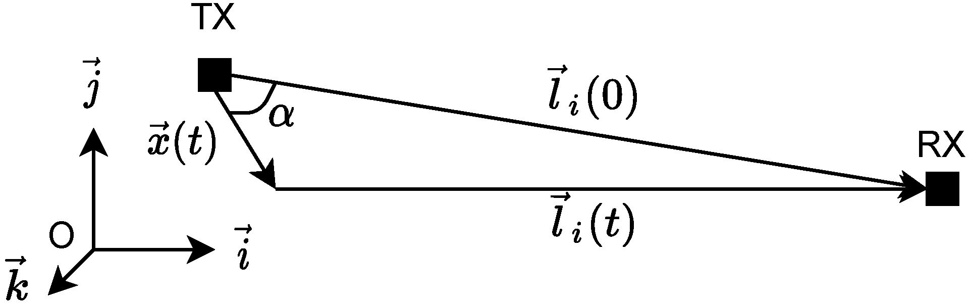
2.2. Geometrical Modeling
- : the signal delay depending on time with ;
- : a loss term due to propagation depending on .
- Hypothesis 1: , i.e., the transmitter movement is negligible compared to the initial distance between the transmitter and receiver during signal observation time T.
- Hypothesis 2: , i.e., the distance between the transmitter and receiver at time is approximately the same as at time t.
- Hypothesis 3: Depending of the movement , one of the two following sub-hypotheses should be chosen:
- -
- Hypothesis 3a: In case of an arbitrary movement , the loss term is considered constant, i.e., the loss term is considered independent of (stronger hypothesis but more general);
- -
- Hypothesis 3b: In case of a small movement (), , i.e., the product of the wavenumber and the initial distance is much greater than 1 (weaker hypothesis but less general).
- : a constant loss term due to propagation;
- : the initial delay;
- : the unitary vector of ;
- : the initial phase.
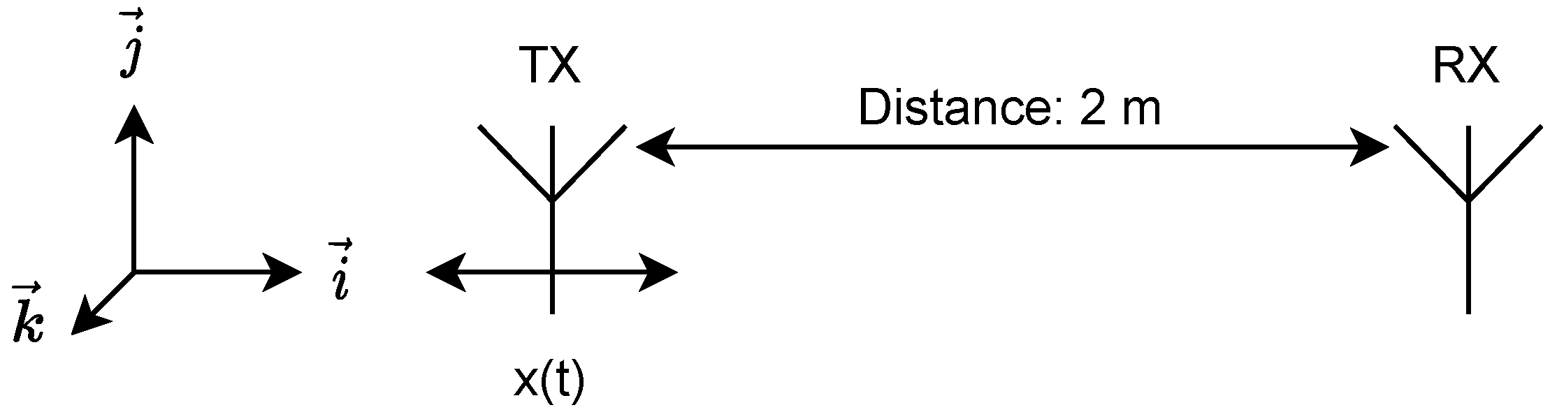
2.3. Testbed and Experiments
2.3.1. Testbed, Hypothesis and Formalization
- Hypothesis:
- -
- Isotropic antenna transmitting a sinusoid:;
- -
- The micro-movement is a sinusoid:;
- -
- Resulting baseband signal (Jacobi–Anger expansion):
- Transmitting system:
- -
- Sinusoid generator: ANRITSU MG3692B;
- -
- Transmitting antenna: Ettus VERT 2450;
- -
- Vibration generator: WOVELOT 037606, nominal voltage 1.5 V;
- -
- IMU (inertial measurement unit): SparkFun 9DoF Razor IMU M0.
- Receiving system:
- -
- Signal recorder/signal analyzer: Signal Hound BB60C;
- -
- Receiving antenna: Ettus VERT 2450.
- Testing parameters:
- -
- Frequency: 2.45 GHz (affecting );
- -
- Voltage of vibration generator: 1.5 V (affecting and );
- -
- Distance: 2 m (affecting A).
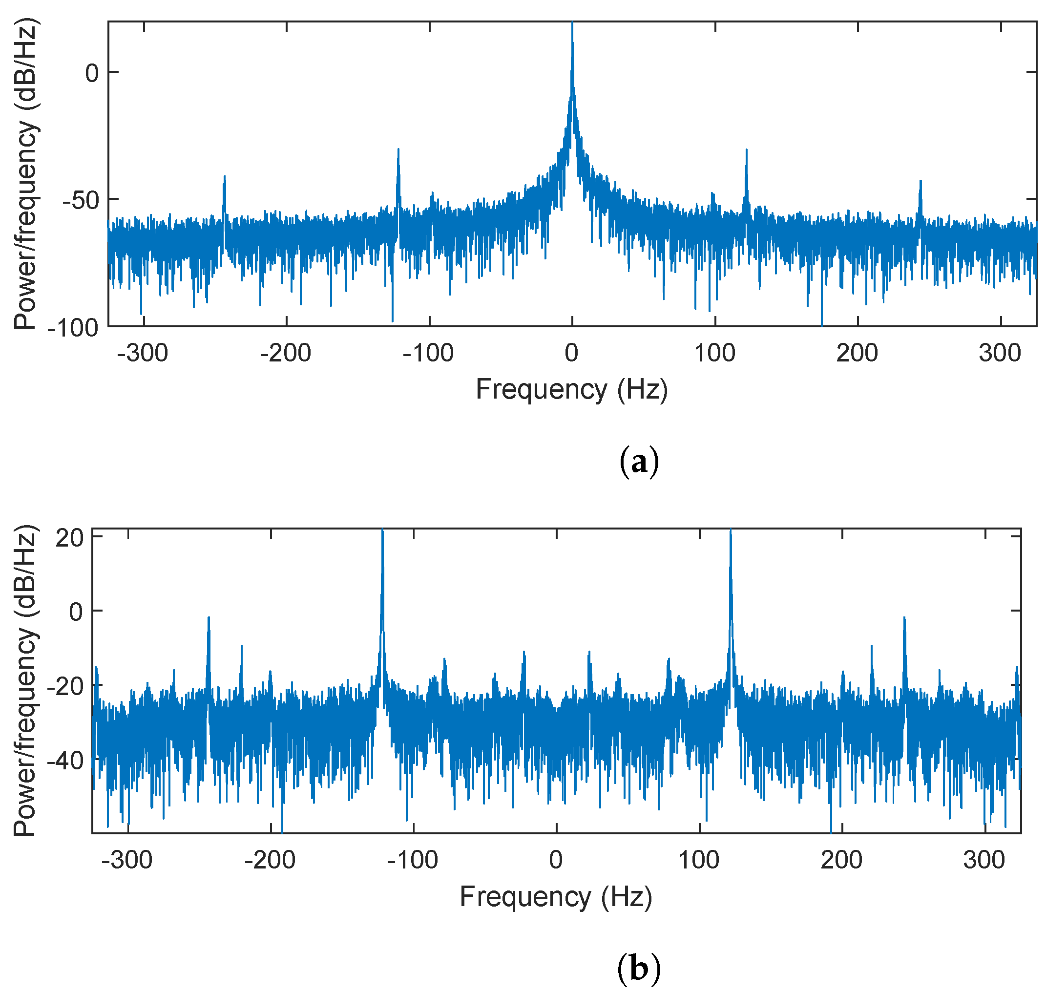
2.3.2. Results
3. Communication Signal Cancellation
3.1. Theoretical Explanations
- A: the amplitude of the signal;
- the MPSK signal;
- M: the modulation order;
- : the rectangular function;
- : the symbol period;
- : an additive white Gaussian complex noise.
3.2. Testbed and Experiment
3.2.1. Testbed, Hypothesis and Formalization
- Hypothesis:
- -
- Isotropic antenna transmitting a 2-PSK:
- -
- The micro-movement is a sinusoid:
- -
- Resulting baseband signal:
- Transmitting system:
- -
- Signal generator: ANRITSU MS2830A;
- -
- Transmitting antenna: Ettus VERT 2450;
- -
- Vibration generator: WOVELOT 178037606, nominal voltage 1.5 V.
- Receiving system:
- -
- Signal recorder/Signal Analyzer: Signal Hound BB60C;
- -
- Receiving antenna: Ettus VERT 2450.
- Testing parameters:
- -
- Frequency: 2.45 GHz;
- -
- Voltage of vibration generator: 1.5 V;
- -
- Distance: 2 m;
- -
- Modulation: BPSK (rectangular pulse shaping).
3.2.2. Results
4. Signal Model, Detection and Estimation
4.1. Signal Model of Doppler Modulation
- ,
- : the total frequency offset taking into account the Doppler shift and the frequency offset between transmitter and receiver;
- : an additive white Gaussian complex noise.
- : a Fourier series coefficient.
- : the spectrum of the additive white Gaussian complex noise.
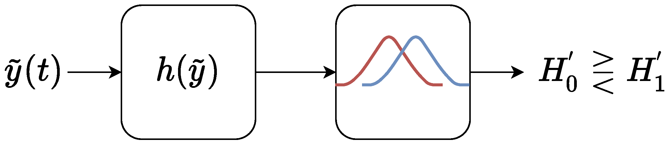
4.2. Detection Method
4.2.1. Theoretical Explanations
- : the spectral coherence;
- : the cyclic frequency (here equivalent to ).
- : the estimated frequency offset using Fourier transform as mentioned by [26].
- assumed to be an additive white Gaussian complex noise.
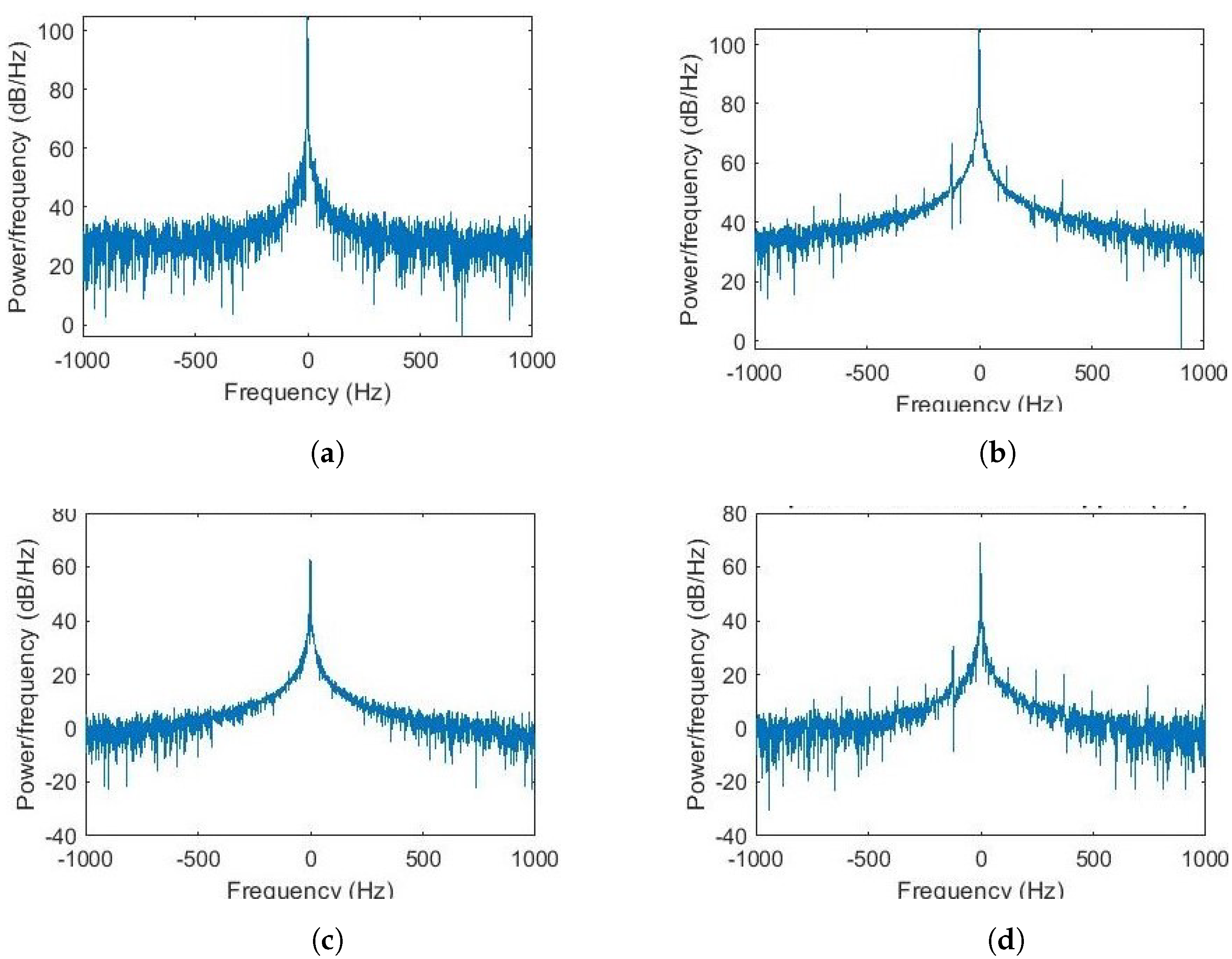
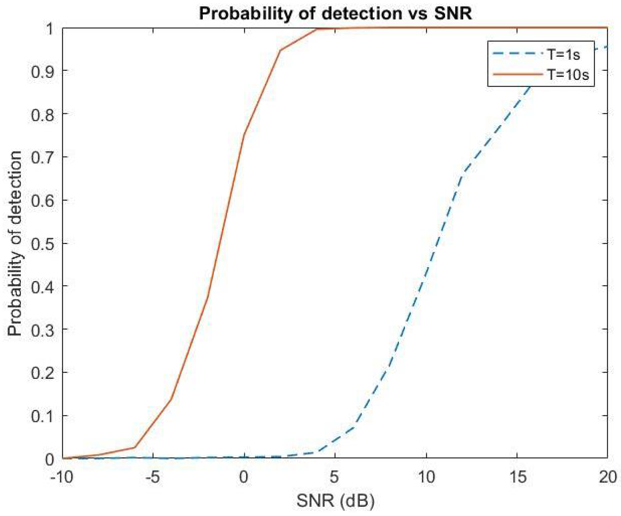
4.2.2. Results
- : the modulation index;
- : the periodic frequency;
- : the frequency offset;
- : the additive white Gaussian complex noise.

4.3. Estimation Algorithm
4.3.1. Spectral Estimation Techniques
- Classical spectral estimation: these methods are called non-parametric methods because they do not require a priori information on the studied signal. One of the most famous methods is the periodogram based on the discrete Fourier transform.
- High-resolution methods: these methods are based on line spectrum (multiple tones) with additive white Gaussian noise. The main methods are: AR, Capon, and sub-space methods (MUSIC, ESPRIT.). The sub-space methods are particularly robust to noise.
- Sparse approximation: the sparsity consists of a signal to decompose it as a small number of atoms. These atoms can be part of a Fourier basis, wavelet basis, or other dictionaries (k-SVD, etc.). There exist many methods for estimating the different components such as basis pursuit, matching pursuit or thresholding techniques.
- Specific estimation techniques: it is possible to use an estimation technique that consists of the estimation of the parameters of a signal. For example, Niu et al. [30] proposed an estimation technique for sinusoidal frequency-modulated (SFM) signal. Note that SFM is a special case of our signal model where and .
4.3.2. Proposed Algorithm
- : the vector containing the signal ();
- : the dictionary () containing the different tones ;
- : a vector containing the nth tone signal,
- the sampling time;
- : the amplitude vector containing the tones amplitude;
- : the vector containing the additive white Gaussian complex noise.
| Algorithm 1: Proposed algorithm |
| Result: The periodic frequency , the central frequency and the amplitudes Estimate Estimate Construct the dictionary D; Estimate . |
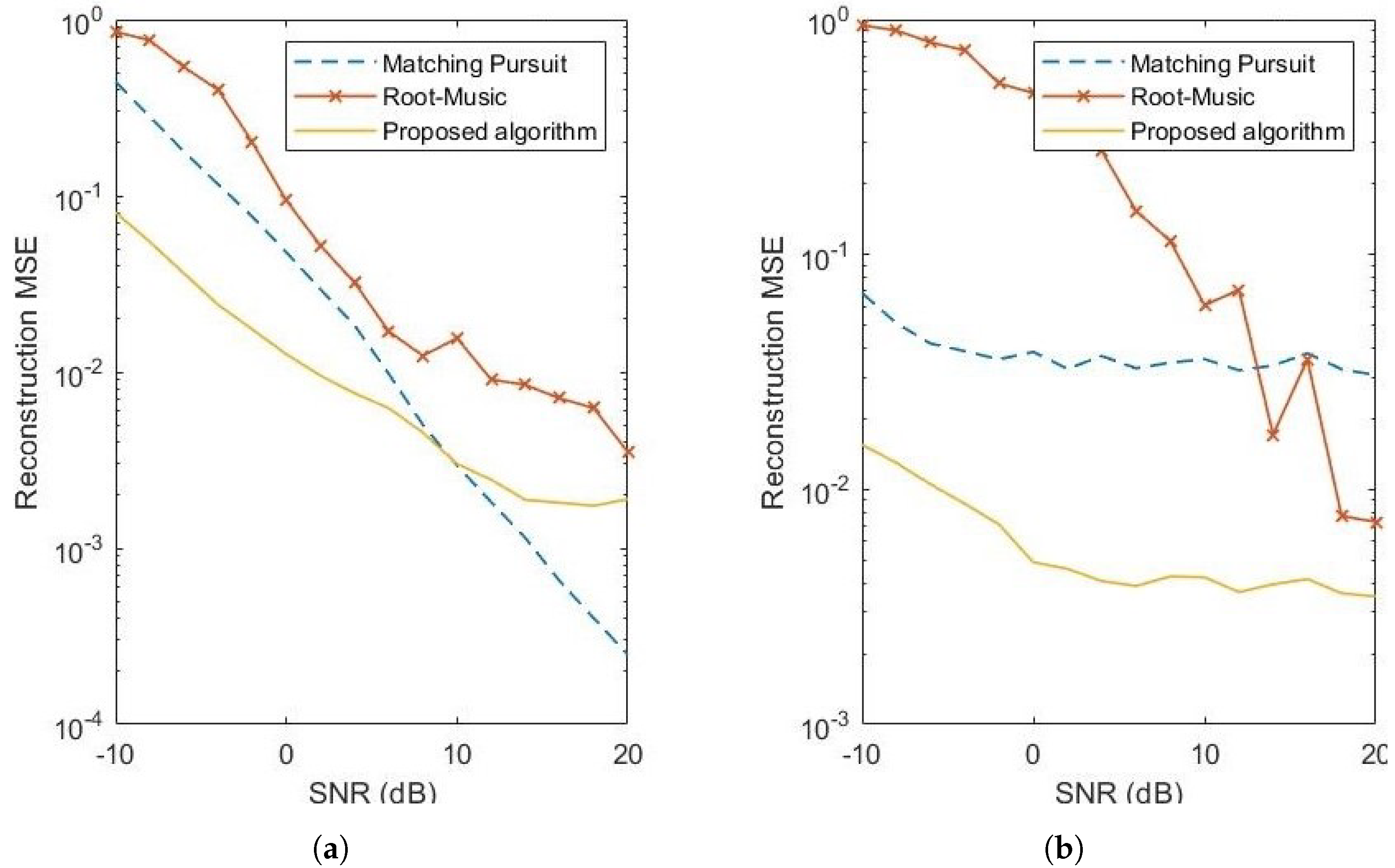
4.3.3. Results
- : the modulation index;
- : the periodic frequency;
- : the frequency offset;
- : the additive white Gaussian complex noise.
- Matching pursuit: a sparse approximation algorithm using a greedy approach [33]. The dictionary used for sparse approximation is a Fourier redundant dictionary with frequency spacing of 0.1 Hz.
- Root-MUSIC: a high-resolution algorithm using noise subspace properties [32]. We use the “rootmusic” Matlab function to estimate the different frequency components.
- L: the signal length;
- : the signal ;
- D: the dictionary used for estimation (depending of the method);
- : the estimated weight.
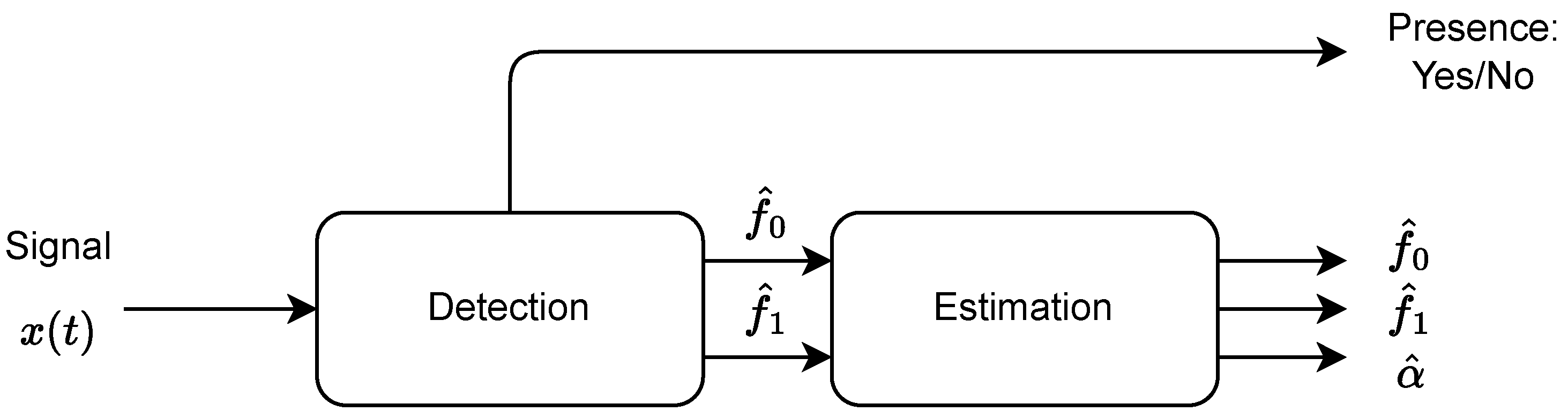
4.4. Hybrid Detection/Estimation Procedure
5. Future Use Cases
5.1. Simulation
5.2. Vibration Object Detection
5.3. RF Fingerprinting
5.4. Vibration Analysis
6. Conclusions
Author Contributions
Funding
Data Availability Statement
Acknowledgments
Conflicts of Interest
Appendix A. Doppler Modulation: Geometrical Modeling Simplifications
Appendix A.1. Step 1: Geometrical Simplification
Appendix A.2. Step 2: Signal Simplification
- : the received power;
- : the transmitted power;
- : the transmitter antenna gain;
- : the receiver antenna gain.
Appendix A.3. Step 3: Neglecting the Amplitude Modulation Due to Motion
- : an amplitude modulation
- : a phase modulation.
- .
Appendix B. Noise Modeling for Signal Cancellation Method
- Proof showing that the term is a white Gaussian complex noise;
- Proof showing that the term is negligible compared to .
Appendix B.1. Properties of the First Term of the Noise
Appendix B.2. Neglecting the Second Part of the Noise
Appendix C. Modified Binary Hypothesis Test
Appendix C.1. Initial Binary Hypothesis Test
- the spectral coherence,
- the cyclic frequency (here equivalent to ).
- : A modulation among DSB-SC AM, BPSK, b-FSK, MSK and QPSK (or cyclostationary signals [25]);
- : An additive white Gaussian complex noise (AWGN).
Appendix C.2. Modified Hypothesis Test

References
- Tse, D. Fundamentals of Radio Communications; Cambridge University Press: Cambridge, UK, 2005. [Google Scholar]
- Brossier, J.-M.; Jourdain, J. Algorithmes Adaptatifs Auto-Optimisés Pour l’égalisation et la Récupération de Porteuse Application aux Transmissions Acoustiques Sous-Marines. Trait. Signal 1994, 11, 327–336. [Google Scholar]
- Simon, E. Estimation de Canal et Synchronisation Pour les Systèmes OFDM en Présence de Mobilité. Ph.D. Thesis, HdR, Institut d’Electronique de Microélectronique et de Nanotechnologie, Université de Lille, Lillen, France, 2005. [Google Scholar]
- Clarke, J.H. A statistical theory of mobile-radio reception. Bell Syst. Tech. J. 1968, 47, 957–1000. [Google Scholar] [CrossRef]
- Lyonnet, B. Diversité Spatiale et Compensation Doppler en Communication Sous-Marine sur Signaux Large-Bandes. Ph.D. Thesis, Grenoble-INP, Grenoble, France, 2011. [Google Scholar]
- Mours, A. Localisation de Cible en Sonar Actif. Ph.D. Thesis, Grenoble-INP, Grenoble, France, 2017. [Google Scholar]
- Doppler, C. On the Coloured Light of the Binary Stars and Some Other Stars of the Heavens—Attempt at a General Theory including Bradley’s Theorem as an Integral Part. Proc. R. Bohemian Soc. Sci. Prague (Part V) 1842, 465, 482. [Google Scholar]
- Chen, V.C.; Ling, H. Time-Frequency Transforms for Radar Imaging and Signal Analysis; Artech House: Norwood, MA, USA, 2002; pp. 173–192. [Google Scholar]
- Chen, V.C.; Li, F.; Ho, S.-S.; Wechsler, H. Micro-Doppler Effect in Radar: Phenomenon, Model, and Simulation Study. IEEE Trans. Aerosp. Electron. Syst. 2006, 42, 2–21. [Google Scholar] [CrossRef]
- de Wit, J.J.M.; Harmanny, R.I.A.; Prémel-Cabic, G. Micro-Doppler Analysis of Small UAVs. In Proceedings of the 2012 9th European Radar Conference, Amsterdam, The Netherlands, 31 October–2 November 2012. [Google Scholar]
- Chen, V.C. The Micro-Doppler Effect in Radar; Artech House: Norwood, MA, USA, 2019. [Google Scholar]
- Sun, W.; Chen, T.; Zheng, J.; Lei, Z.; Wang, L.; Steeper, B.; He, P.; Dressa, M.; Tian, F.; Zhang, C. VibroSense: Recognizing Home Activities by Deep Learning Subtle Vibrations on an Interior Surface of a House from a Single Point Using Laser Doppler Vibrometry. Proc. ACM Interact. Mobile Wearable Ubiquitous Technol. 2020, 4, 96. [Google Scholar] [CrossRef]
- Nguyen, P.; Truong, H.; Ravindranathan, M.; Nguyen, A.; Han, R.; Vu, T. Matthan: Drone Presence Detection by Identifying Physical Signatures in the Drone’s RF Communication. In Proceedings of the 15th Annual International Conference on Mobile Systems, Applications, and Services, Niagara Falls, NY, USA, 19–23 June 2017; pp. 211–224. [Google Scholar]
- Basnayaka, D.A.; Ratnarajah, T. Doppler Effect Assisted Wireless Communication for Interference Mitigation. IEEE Trans. Commun. 2019, 67, 5203–5212. [Google Scholar] [CrossRef] [Green Version]
- Fu, H.; Abeywickrama, S.; Lihao, Z.; Yen, C. Low-Complexity Portable Passive Drone Surveillance via SDR-Based Signal Processing. IEEE Commun. Mag. 2018, 56, 112–118. [Google Scholar] [CrossRef]
- Yang, X.; Huo, K.; Jiang, W.; Zhao, J.; Qiu, Z. A passive radar system for detecting UAV based on the OFDM communication signal. In Proceedings of the 2016 Progress in Electromagnetic Research Symposium (PIERS), Shanghai, China, 8–11 August 2016. [Google Scholar]
- Clemente, C.; Soraghan, J.J. GNSS-Based Passive Bistatic Radar for Micro-Doppler Analysis of Helicopter Rotor Blades. IEEE Trans. Aerosp. Electron. Syst. 2014, 50, 491–500. [Google Scholar] [CrossRef]
- Li, K.-M.; Qu, X.-Y.; Wu, Y.; Xia, Y.-H.; Li, W.-Y. A Method for Micro-Doppler Extraction Under Passive Radar Based on Communiction Signal. In Proceedings of the IGARSS 2019—2019 IEEE International Geoscience and Remote Sensing Symposium, Yokohama, Japan, 28 July–2 August 2019. [Google Scholar]
- Papoulis, A.; Pillai, U. Probability, Random Variables and Stochastic Processes, 4th ed.; McGraw-Hill Higher Education: New York, NY, USA, 2002. [Google Scholar]
- Bauduin, G. Radiocommunications Numériques—Tome 1; Dunod: Paris, France, 2013. [Google Scholar]
- McCormick, A.C.; Nandi, A.K. Cyclostionarity in Rotating Machine Vibrations. Mech. Syst. Signal Process. 1998, 12, 225–242. [Google Scholar] [CrossRef] [Green Version]
- Glavieux, A. Introduction aux Communications Numériques; Chapter 7; Dunod: Paris, France, 2007. [Google Scholar]
- Stoica, P.; Moses, R. Spectral Analysis of Signals; Chapter 4; Prentice Hall: Upper Saddle River, NJ, USA, 2004. [Google Scholar]
- Kim, K.; Akbar, I.A.; Bae, K.K.; Um, J.-S.; Spooner, C.M.; Reed, J.H. Cyclostationary Approaches to Signal Detection and Classification in Cognitive Radio. In Proceedings of the 2007 2nd IEEE International Symposium on New Frontiers in Dynamic Spectrum Access Networks, Dublin, Ireland, 17–20 April 2007. [Google Scholar]
- Chen, J.; Gibson, A.; Zafar, Z. Cyclostationary Spectrum Detection in Cognitive Radios. In Proceedings of the 2008 IET Seminar on Cognitive Radio and Software Defined Radios: Technologies and Techniques, London, UK, 18 September 2008. [Google Scholar]
- Blanchet, G.; Charbit, M. Signaux et Images sous Matlab. Méthodes, Applications et Exercices Corrigés; Hermès: Paris, France, 2001. [Google Scholar]
- Antoni, J.; Xin, G.; Hamzaoui, M. Fast Computation of the Spectral Correlation. Mech. Syst. Signal Process. 2017, 92, 248–277. [Google Scholar] [CrossRef]
- Antoni, J. Fast Spectral Correlation Matlab Implementation. 2021. Available online: https://www.mathworks.com/matlabcentral/fileexchange/60561-fast_sc-x-nw-alpha_max-fs-op (accessed on 11 February 2021).
- Sapiro, G. Image and Video Processing: From Mars to Hollywood with a Stop at the Hospital. Sparse Modeling (p066), Coursera. 2013. Available online: https://www.youtube.com/watch?v=eq-itFq0Sco&ab_channel=AlanSaberi (accessed on 11 February 2021).
- Niu, J.; Zhu, Y.; Liu, Y.; Li, X.; Kuang, G. Parameter estimation of a sinusoidal FM signal using CAF-MR algorithm. In Proceedings of the 2012 IEEE International Conference on Information Science and Technology, Wuhan, China, 23–25 March 2012. [Google Scholar]
- Mototolea, D.; Youssef, R.; Radoi, E.; Nicolaescu, I. Non-cooperative low-complexity detection approach for FHSS-GFSK drone control signals. IEEE Open J. Commun. Soc. 2020, 1, 401–412. [Google Scholar] [CrossRef]
- Badeau, R. Méthodes à Haute Résolution pour l’estimation et le Suivi de Sinusoïdes Modulées. Application aux Signaux de Musique. Ph.D. Thesis, Ecole Nationale Supérieure des Télécommunications, Paris, France, 2005. [Google Scholar]
- Mallat, S.G.; Zhang, Z. Matching pursuits with time-frequency dictionaries. IEEE Trans. Signal Process. 1993, 41, 3397–3415. [Google Scholar] [CrossRef]
- Brik, V.; Banerjee, S.; Gruteser, M.; Oh, S. Wireless Device Identification with Radiometric Signatures. In Proceedings of the 14th ACM International Conference on Mobile Computing and Networking, San Francisco, CA, USA, 14–19 September 2008; pp. 116–127. [Google Scholar]


Publisher’s Note: MDPI stays neutral with regard to jurisdictional claims in published maps and institutional affiliations. |
© 2022 by the authors. Licensee MDPI, Basel, Switzerland. This article is an open access article distributed under the terms and conditions of the Creative Commons Attribution (CC BY) license (https://creativecommons.org/licenses/by/4.0/).
Share and Cite
Morge-Rollet, L.; Le Jeune, D.; Le Roy, F.; Canaff, C.; Gautier, R. From Modeling to Sensing of Micro-Doppler in Radio Communications. Remote Sens. 2022, 14, 6310. https://doi.org/10.3390/rs14246310
Morge-Rollet L, Le Jeune D, Le Roy F, Canaff C, Gautier R. From Modeling to Sensing of Micro-Doppler in Radio Communications. Remote Sensing. 2022; 14(24):6310. https://doi.org/10.3390/rs14246310
Chicago/Turabian StyleMorge-Rollet, Louis, Denis Le Jeune, Frédéric Le Roy, Charles Canaff, and Roland Gautier. 2022. "From Modeling to Sensing of Micro-Doppler in Radio Communications" Remote Sensing 14, no. 24: 6310. https://doi.org/10.3390/rs14246310