
Improving Spatial Resolution of Satellite Imagery Using Generative Adversarial Networks and Window Functions

Abstract
:1. Introduction
- Are there any methods to combine images after the application of algorithms to improve spatial resolution with the use of deep learning methods?
- What methodology should be adopted to combine images evaluated by generative adversarial networks?
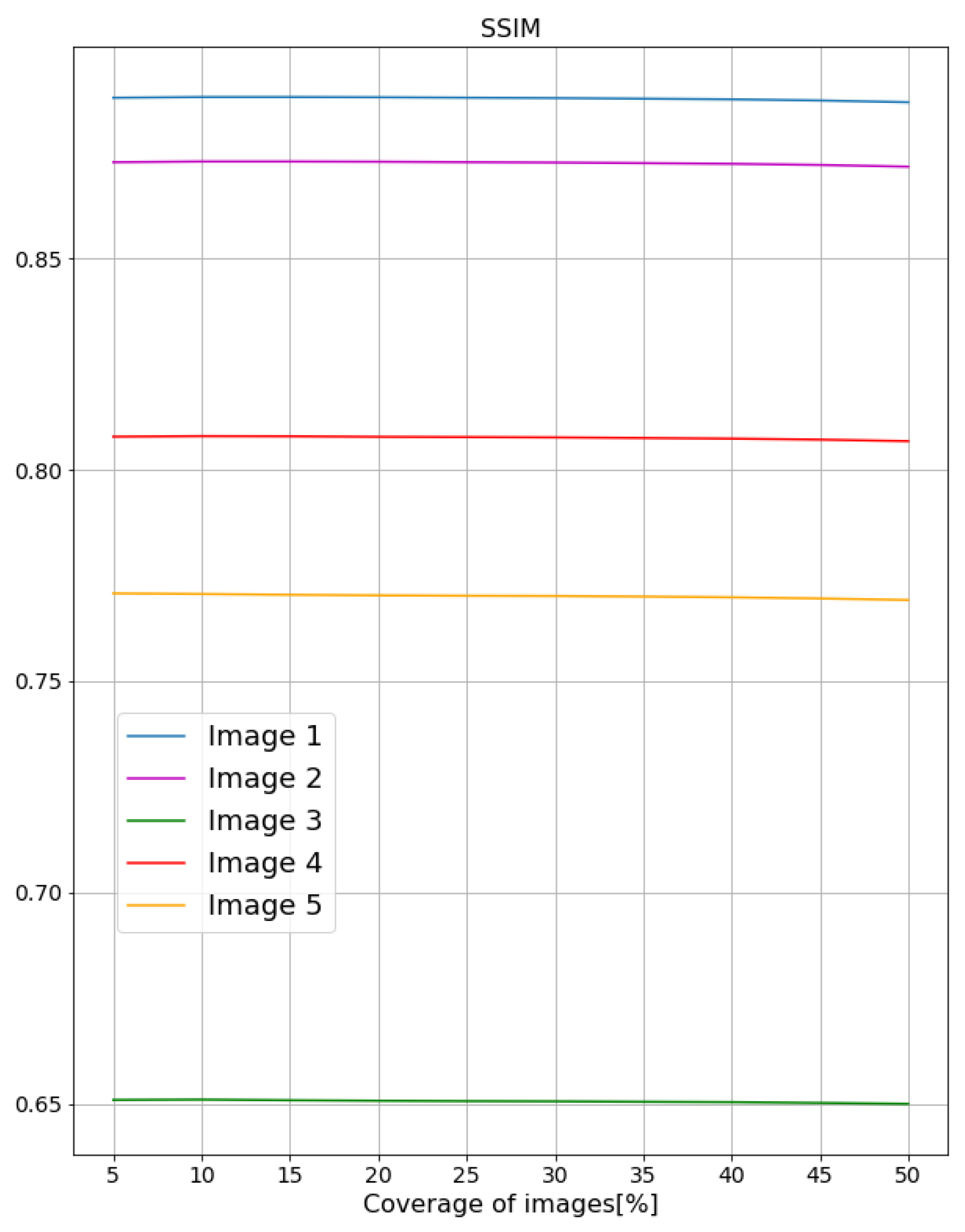
- What is the number of buffer pixels that will result in the best quality of the resulting image?
- Can this method also be used to combine images that are the outcome of segmentation algorithms?
2. Related Works
3. Experiments and Results
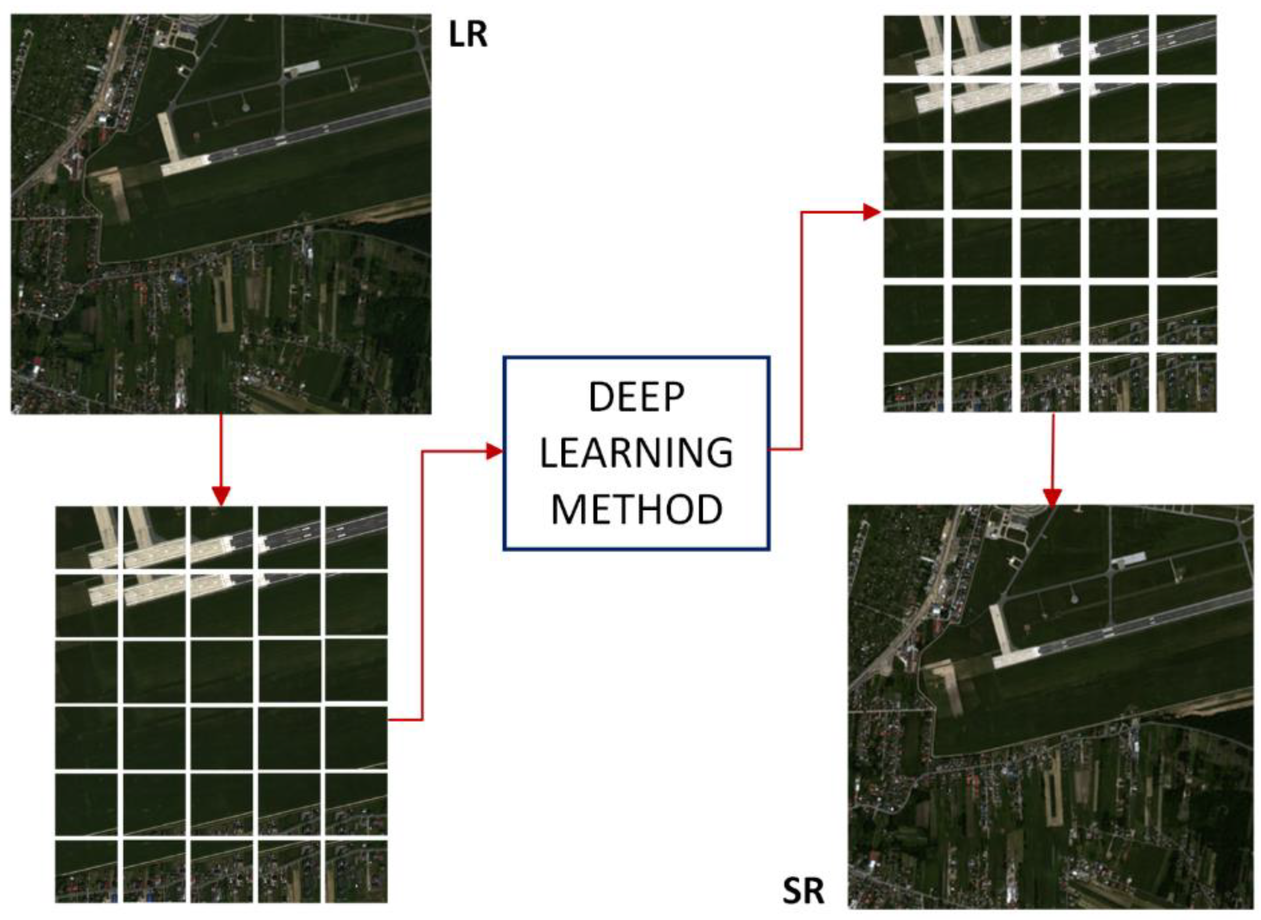
3.1. The Proposed Method
3.2. Equations
3.2.1. Peak Signal-to-Noise Ratio
3.2.2. Universal Quality Measure
3.2.3. Spatial Correlation Coefficient
3.2.4. Spectral Angle Mapper
3.2.5. Spectral Angle Mapper
3.2.6. VIFP
3.2.7. Normalized Root Mean-Squared Error
3.2.8. Mean Square Error
3.2.9. Root Mean Square Error
3.3. Preliminary Tests
3.4. Results
3.4.1. Database
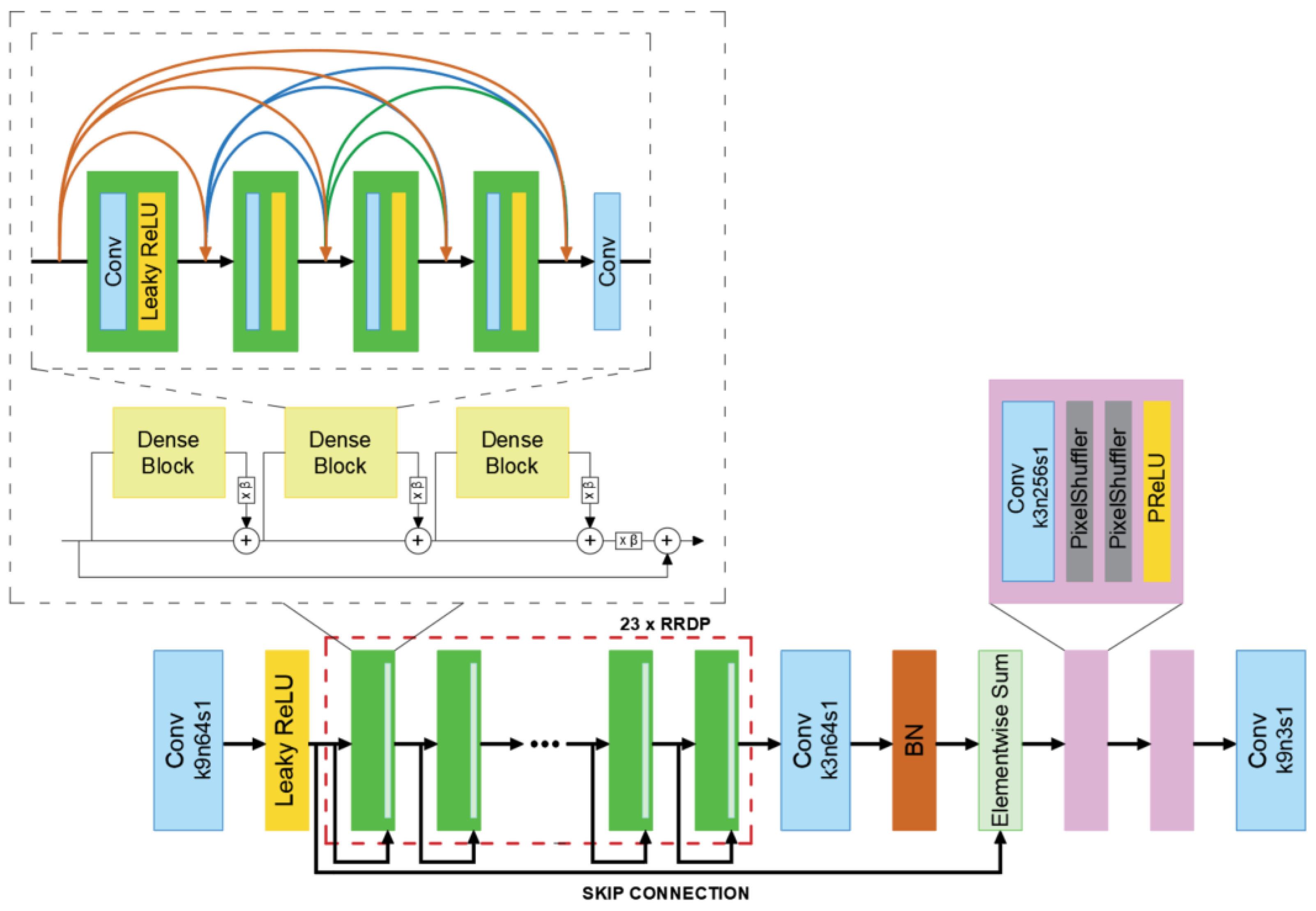
3.4.2. The ESRGAN Network
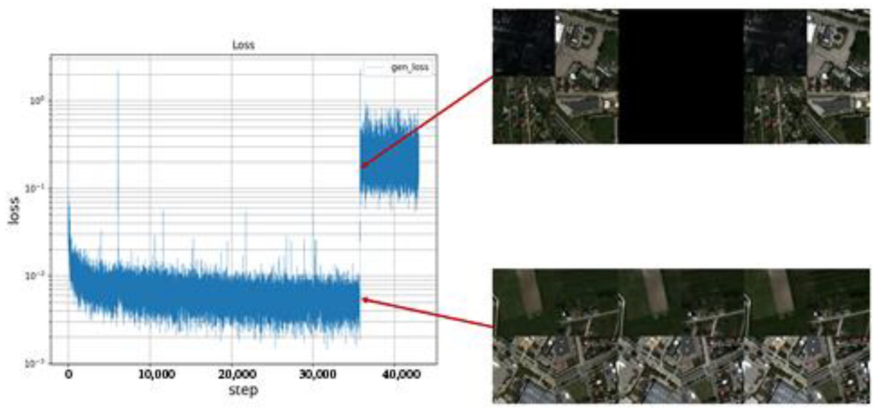
3.4.3. Network Training
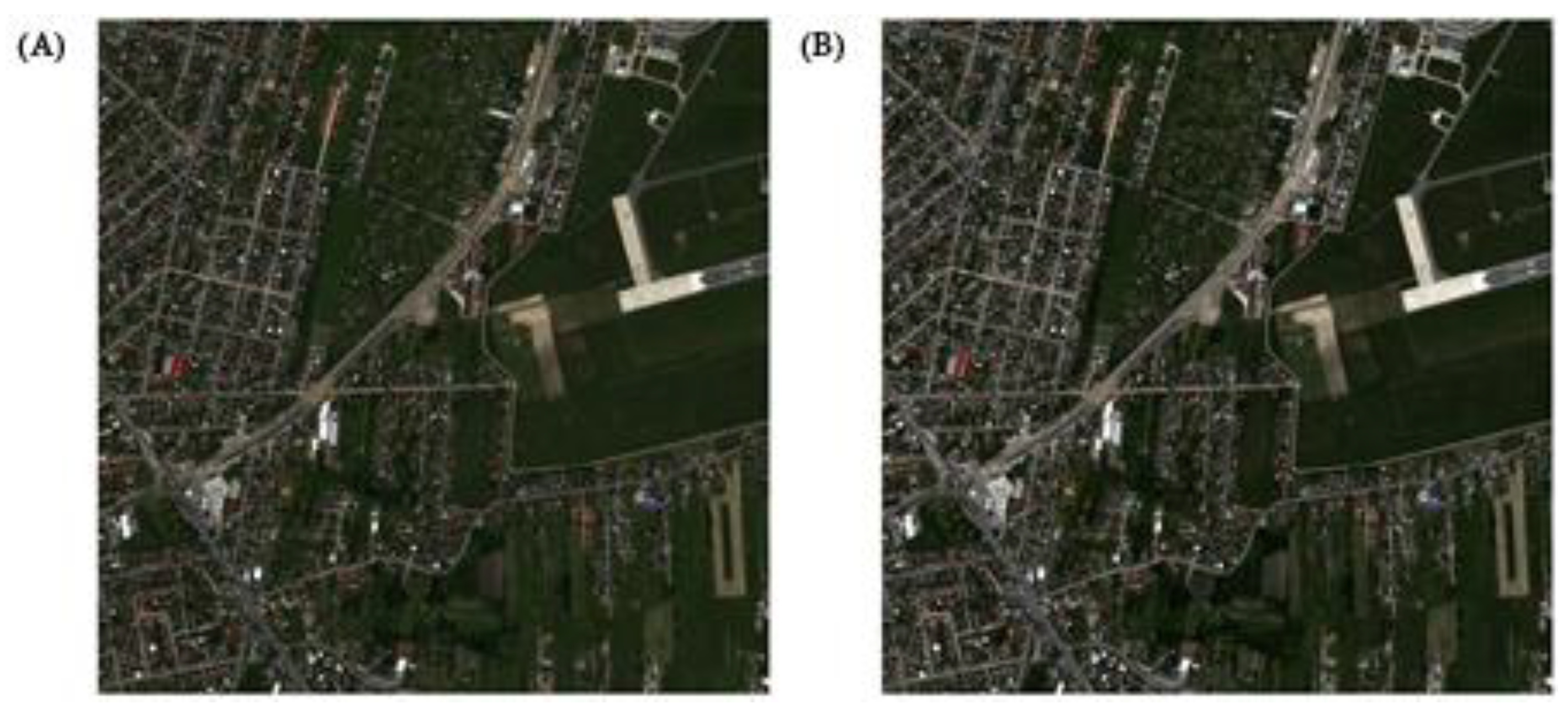
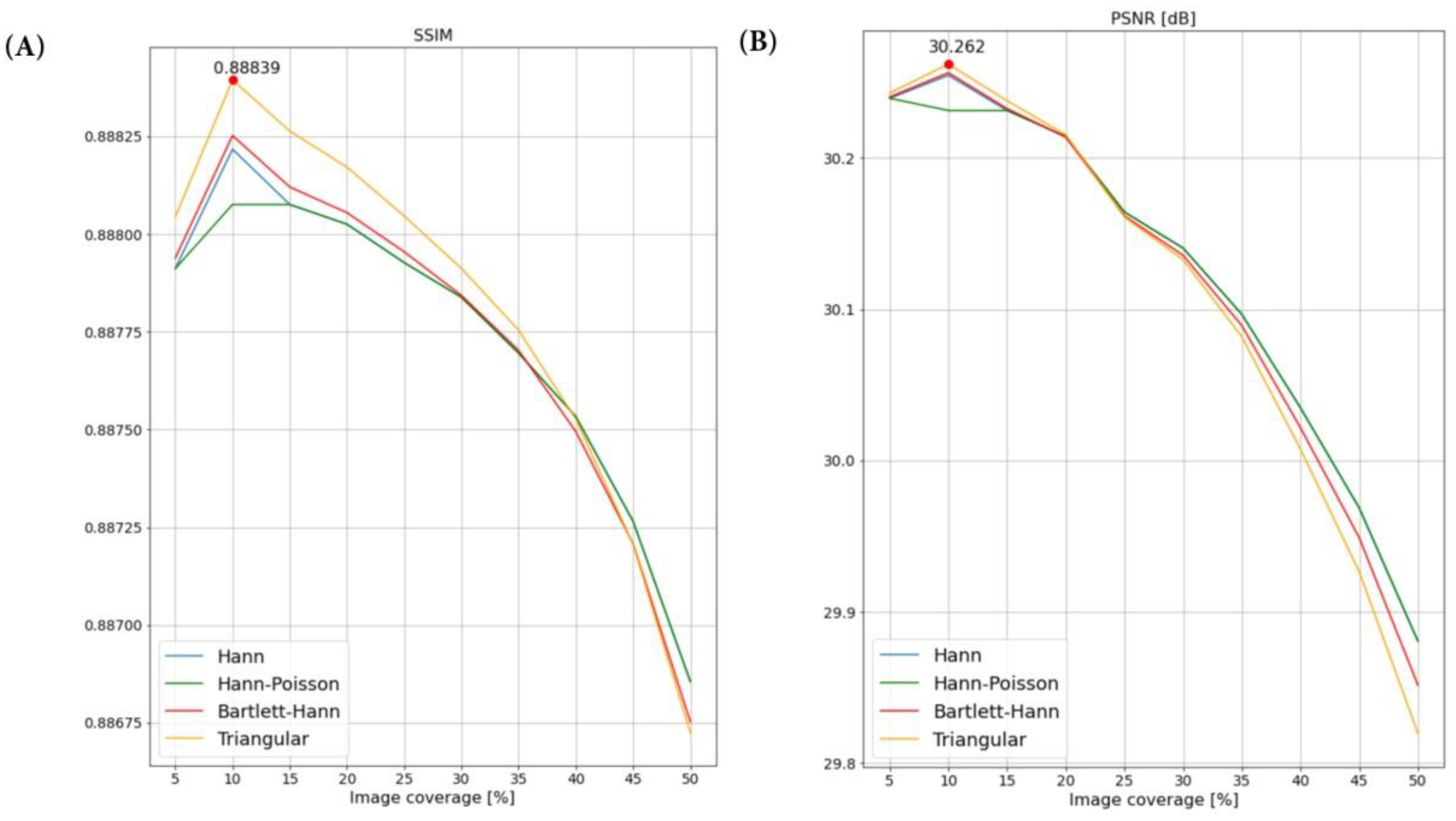
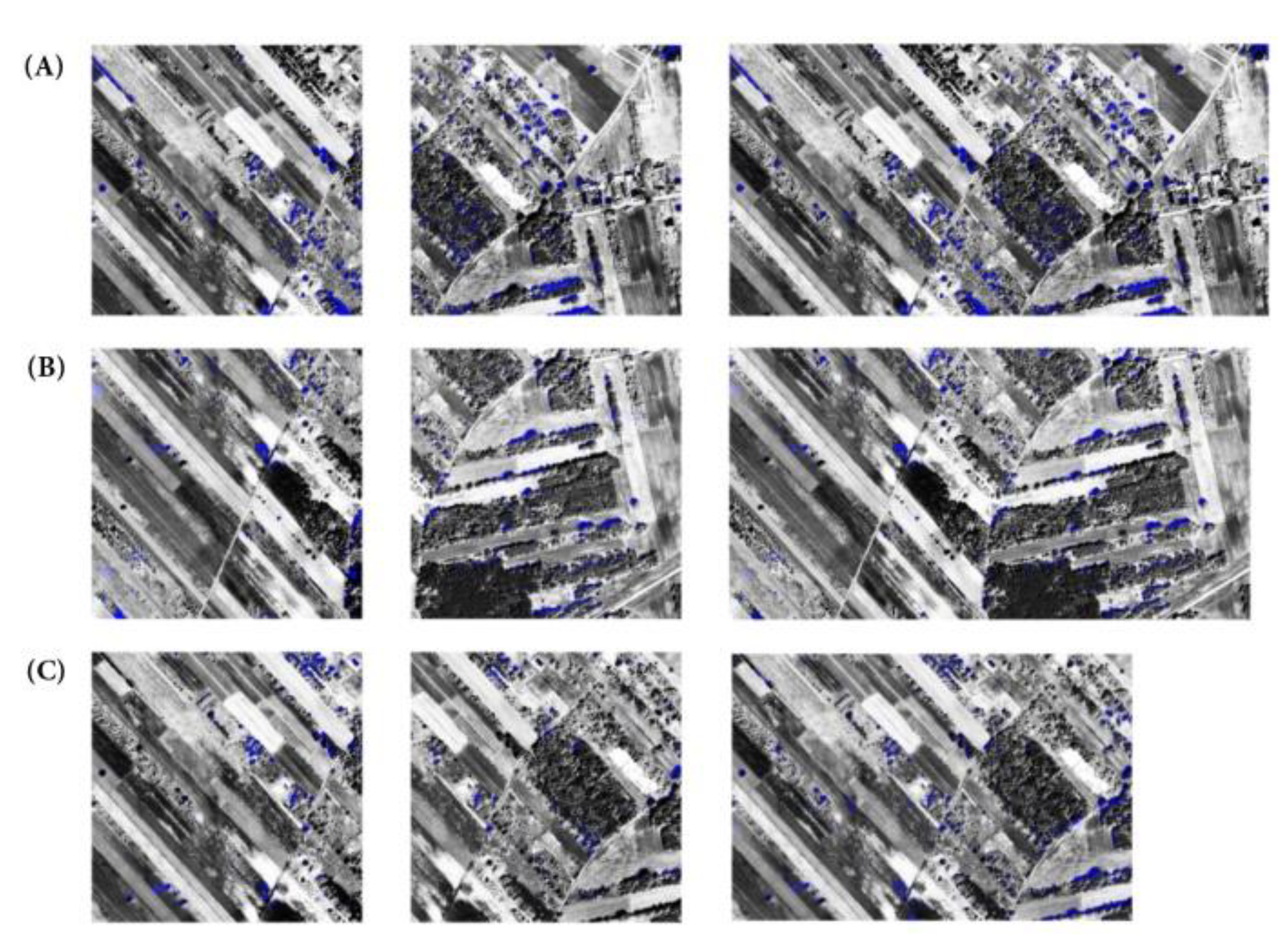
3.4.4. Combining Images
4. Discussion
5. Conclusions
Author Contributions
Funding
Conflicts of Interest
Appendix A

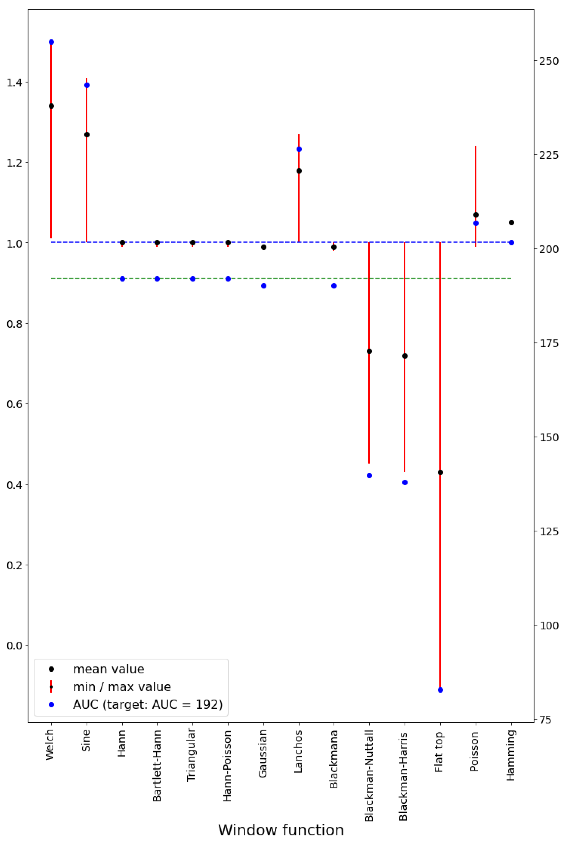
| WINDOW | Formula | Min | Max | Mean | Surface for Image 384 pix | Figure (the Modification, When in Non-Overlapping Areas, i.e., on the External Edges, the Value of the Window Function Equals 1) Image Overlap of 50% Was Assumed. |
|---|---|---|---|---|---|---|
| Welch | 1.01 | 1.50 | 1.34 | 254.99 |  | |
| Sine | 1.00 | 1.41 | 1.27 | 243.46 |  | |
| Hann | 0.9 (9) | 1.00 | 1.00 | 192 |  | |
| Bartlett-Hann | 0.9 (9) | 1.00 | 1.00 | 192 |  | |
| Triangular | 0.9 (9) | 1.00 | 1.00 | 192 |  | |
| Hann-Poisson | 0.9 (9) | 1.00 | 1.00 | 192 |  | |
| Gaussian | Selected: | 0.92 | 1.05 | 0.99 | 190.11 |  |
| Lanchos | 1.0 | 1.27 | 1.18 | 226.36 |  | |
| Blackmana | Selected: | 0.98 | 1.00 | 0.99 | 190.08 |  |
| Blackman-Nuttall | 0.45 | 1.00 | 0.73 | 139.62 |  | |
| Blackman–Harris window | 0.43 | 1.00 | 0.72 | 137.76 |  | |
| Flat top window | −0.11 | 1.0 | 0.43 | 82.78 |  | |
| Exponential or Poisson window | 0.99 | 1.24 | 1.07 | 206.65 |  | |
| Hamming | 1.05 | 1.05 | 1.05 | 201.60 |  |
Appendix B
 |  |  |
 |  |  |
References
- Liu, Y.; Li, Q.; Yuan, Y.; Du, Q.; Wang, Q. ABNet: Adaptive Balanced Network for Multiscale Object Detection in Remote Sensing Imagery. IEEE Trans. Geosci. Remote Sens. 2022, 60, 1–14. [Google Scholar] [CrossRef]
- Cao, Z.; Fang, W.; Song, Y.; He, L.; Song, C.; Xu, Z. DNN-Based Peak Sequence Classification CFAR Detection Algorithm for High-Resolution FMCW Radar. IEEE Trans. Geosci. Remote Sens. 2022, 60, 1–15. [Google Scholar] [CrossRef]
- Cui, Y.; Hou, B.; Wu, Q.; Ren, B.; Wang, S.; Jiao, L. Remote Sensing Object Tracking With Deep Reinforcement Learning Under Occlusion. IEEE Trans. Geosci. Remote Sens. 2022, 60, 1–13. [Google Scholar] [CrossRef]
- Oveis, A.H.; Giusti, E.; Ghio, S.; Martorella, M. A Survey on the Applications of Convolutional Neural Networks for Synthetic Aperture Radar: Recent Advances. IEEE Aerosp. Electron. Syst. Mag. 2022, 37, 18–42. [Google Scholar] [CrossRef]
- Singh, A.; Kalke, H.; Loewen, M.; Ray, N. River Ice Segmentation With Deep Learning. IEEE Trans. Geosci. Remote Sens. 2020, 58, 7570–7579. [Google Scholar] [CrossRef] [Green Version]
- Saha, S.; Mou, L.; Qiu, C.; Zhu, X.X.; Bovolo, F.; Bruzzone, L. Unsupervised Deep Joint Segmentation of Multitemporal High-Resolution Images. IEEE Trans. Geosci. Remote Sens. 2020, 58, 8780–8792. [Google Scholar] [CrossRef]
- Zhang, B.; Chen, T.; Wang, B. Curriculum-Style Local-to-Global Adaptation for Cross-Domain Remote Sensing Image Segmentation. IEEE Trans. Geosci. Remote Sens. 2022, 60, 1–12. [Google Scholar] [CrossRef]
- Mei, S.; Jiang, R.; Li, X.; Du, Q. Spatial and Spectral Joint Super-Resolution Using Convolutional Neural Network. IEEE Trans. Geosci. Remote Sens. 2020, 58, 4590–4603. [Google Scholar] [CrossRef]
- Song, H.; Huang, B.; Liu, Q.; Zhang, K. Improving the Spatial Resolution of Landsat TM/ETM+ Through Fusion With SPOT5 Images via Learning-Based Super-Resolution. IEEE Trans. Geosci. Remote Sens. 2015, 53, 1195–1204. [Google Scholar] [CrossRef]
- Lima, P.; Steger, S.; Glade, T.; Murillo-García, F.G. Literature Review and Bibliometric Analysis on Data-Driven Assessment of Landslide Susceptibility. J. Mt. Sci. 2022, 19, 1670–1698. [Google Scholar] [CrossRef]
- Xia, D.; Tang, H.; Sun, S.; Tang, C.; Zhang, B. Landslide Susceptibility Mapping Based on the Germinal Center Optimization Algorithm and Support Vector Classification. Remote Sens. 2022, 14, 2707. [Google Scholar] [CrossRef]
- Wang, L.; Scott, K.A.; Xu, L.; Clausi, D.A. Sea Ice Concentration Estimation During Melt From Dual-Pol SAR Scenes Using Deep Convolutional Neural Networks: A Case Study. IEEE Trans. Geosci. Remote Sens. 2016, 54, 4524–4533. [Google Scholar] [CrossRef]
- Wang, L.; Scott, K.A.; Clausi, D.A. Sea Ice Concentration Estimation during Freeze-Up from SAR Imagery Using a Convolutional Neural Network. Remote Sens. 2017, 9, 408. [Google Scholar] [CrossRef]
- Cooke, C.L.V.; Scott, K.A. Estimating Sea Ice Concentration From SAR: Training Convolutional Neural Networks With Passive Microwave Data. IEEE Trans. Geosci. Remote Sens. 2019, 57, 4735–4747. [Google Scholar] [CrossRef]
- Scarpa, G.; Gargiulo, M.; Mazza, A.; Gaetano, R. A CNN-Based Fusion Method for Feature Extraction from Sentinel Data. Remote Sens. 2018, 10, 236. [Google Scholar] [CrossRef] [Green Version]
- Oveis, A.H.; Giusti, E.; Ghio, S.; Martorella, M. CNN for Radial Velocity and Range Components Estimation of Ground Moving Targets in SAR. In Proceedings of the 2021 IEEE Radar Conference (RadarConf21), Atlanta, GA, USA, 7–14 May 2021; pp. 1–6. [Google Scholar]
- Wang, J.; Lu, C.; Jiang, W. Simultaneous Ship Detection and Orientation Estimation in SAR Images Based on Attention Module and Angle Regression. Sensors 2018, 18, 2851. [Google Scholar] [CrossRef] [Green Version]
- Kuuste, H.; Eenmäe, T.; Allik, V.; Agu, A.; Vendt, R.; Ansko, I.; Laizans, K.; Sünter, I.; Lätt, S.; Noorma, M. Imaging System for Nanosatellite Proximity Operations. Proc. Est. Acad. Sci. 2014, 63, 250. [Google Scholar] [CrossRef]
- Blommaert, J.; Delauré, B.; Livens, S.; Nuyts, D.; Moreau, V.; Callut, E.; Habay, G.; Vanhoof, K.; Caubo, M.; Vandenbussche, J.; et al. CHIEM: A New Compact Camera for Hyperspectral Imaging. 2017. Available online: https://www.researchgate.net/publication/321214165_CHIEM_A_new_compact_camera_for_hyperspectral_imaging (accessed on 18 October 2022).
- Isola, P.; Zhu, J.-Y.; Zhou, T.; Efros, A.A. Image-to-Image Translation with Conditional Adversarial Networks. In Proceedings of the IEEE Conference on Computer Vision and Pattern Recognition, Salt Lake City, UT, USA, 18–22 June 2018. [Google Scholar]
- Karwowska, K.; Wierzbicki, D. Using Super-Resolution Algorithms for Small Satellite Imagery: A Systematic Review. IEEE J. Sel. Top. Appl. Earth Obs. Remote Sens. 2022, 15, 3292–3312. [Google Scholar] [CrossRef]
- Lu, T.; Wang, J.; Zhang, Y.; Wang, Z.; Jiang, J. Satellite Image Super-Resolution via Multi-Scale Residual Deep Neural Network. Remote Sens. 2019, 11, 1588. [Google Scholar] [CrossRef] [Green Version]
- Schmidt, R. Multiple Emitter Location and Signal Parameter Estimation. IEEE Trans. Antennas Propag. 1986, 34, 276–280. [Google Scholar] [CrossRef]
- Simonyan, K.; Zisserman, A. Very Deep Convolutional Networks for Large-Scale Image Recognition. arXiv 2015, arXiv:1409.1556. [Google Scholar]
- Howard, A.G.; Zhu, M.; Chen, B.; Kalenichenko, D.; Wang, W.; Weyand, T.; Andreetto, M.; Adam, H. MobileNets: Efficient Convolutional Neural Networks for Mobile Vision Applications. arXiv 2017, arXiv:1704.04861. [Google Scholar]
- He, K.; Zhang, X.; Ren, S.; Sun, J. Deep Residual Learning for Image Recognition. arXiv 2015, arXiv:1512.03385. [Google Scholar]
- Szegedy, C.; Vanhoucke, V.; Ioffe, S.; Shlens, J.; Wojna, Z. Rethinking the Inception Architecture for Computer Vision. arXiv 2015, arXiv:1512.00567. [Google Scholar]
- Han, J.; Zhang, D.; Cheng, G.; Guo, L.; Ren, J. Object Detection in Optical Remote Sensing Images Based on Weakly Supervised Learning and High-Level Feature Learning. IEEE Trans. Geosci. Remote Sens. 2015, 53, 3325–3337. [Google Scholar] [CrossRef] [Green Version]
- Wang, Z.; Zhang, Y.; Yu, Y.; Zhang, L.; Min, J.; Lai, G. Prior-Information Auxiliary Module: An Injector to a Deep Learning Bridge Detection Model. IEEE J. Sel. Top. Appl. Earth Obs. Remote Sens. 2021, 14, 6270–6278. [Google Scholar] [CrossRef]
- Yu, D.; Ji, S. A New Spatial-Oriented Object Detection Framework for Remote Sensing Images. IEEE Trans. Geosci. Remote Sens. 2021, 60, 1–16. [Google Scholar] [CrossRef]
- Kemker, R.; Luu, R.; Kanan, C. Low-Shot Learning for the Semantic Segmentation of Remote Sensing Imagery. IEEE Trans. Geosci. Remote Sens. 2018, 56, 6214–6223. [Google Scholar] [CrossRef] [Green Version]
- Vinayaraj, P.; Sugimoto, R.; Nakamura, R.; Yamaguchi, Y. Transfer Learning With CNNs for Segmentation of PALSAR-2 Power Decomposition Components. IEEE J. Sel. Top. Appl. Earth Obs. Remote Sens. 2020, 13, 6352–6361. [Google Scholar] [CrossRef]
- Šćepanović, S.; Antropov, O.; Laurila, P.; Rauste, Y.; Ignatenko, V.; Praks, J. Wide-Area Land Cover Mapping With Sentinel-1 Imagery Using Deep Learning Semantic Segmentation Models. IEEE J. Sel. Top. Appl. Earth Obs. Remote Sens. 2021, 14, 10357–10374. [Google Scholar] [CrossRef]
- Feng, Y.; Sun, X.; Diao, W.; Li, J.; Gao, X.; Fu, K. Continual Learning with Structured Inheritance for Semantic Segmentation in Aerial Imagery. IEEE Trans. Geosci. Remote Sens. 2022, 60, 1–17. [Google Scholar] [CrossRef]
- Zuo, Z.; Li, Y. A SAR-to-Optical Image Translation Method Based on PIX2PIX. In Proceedings of the 2021 IEEE International Geoscience and Remote Sensing Symposium IGARSS, Kuala Lumpur, Malaysia, 17–22 July 2021; pp. 3026–3029. [Google Scholar]
- Chen, X.; Chen, S.; Xu, T.; Yin, B.; Peng, J.; Mei, X.; Li, H. SMAPGAN: Generative Adversarial Network-Based Semisupervised Styled Map Tile Generation Method. IEEE Trans. Geosci. Remote Sens. 2021, 59, 4388–4406. [Google Scholar] [CrossRef]
- Kaiser, P.; Wegner, J.D.; Lucchi, A.; Jaggi, M.; Hofmann, T.; Schindler, K. Learning Aerial Image Segmentation from Online Maps. IEEE Trans. Geosci. Remote Sens. 2017, 55, 6054–6068. [Google Scholar] [CrossRef]
- Fu, Y.; Liang, S.; Chen, D.; Chen, Z. Translation of Aerial Image Into Digital Map via Discriminative Segmentation and Creative Generation. IEEE Trans. Geosci. Remote Sens. 2022, 60, 1–15. [Google Scholar] [CrossRef]
- Vandal, T.J.; McDuff, D.; Wang, W.; Duffy, K.; Michaelis, A.; Nemani, R.R. Spectral Synthesis for Geostationary Satellite-to-Satellite Translation. IEEE Trans. Geosci. Remote Sens. 2022, 60, 1–11. [Google Scholar] [CrossRef]
- Ledig, C.; Theis, L.; Huszar, F.; Caballero, J.; Cunningham, A.; Acosta, A.; Aitken, A.; Tejani, A.; Totz, J.; Wang, Z.; et al. Photo-Realistic Single Image Super-Resolution Using a Generative Adversarial Network. arXiv 2017, arXiv:1609.04802. [Google Scholar]
- Wang, X.; Yu, K.; Wu, S.; Gu, J.; Liu, Y.; Dong, C.; Loy, C.C.; Qiao, Y.; Tang, X. ESRGAN: Enhanced Super-Resolution Generative Adversarial Networks. arXiv 2018, arXiv:1809.00219. [Google Scholar]
- Choi, J.-S.; Kim, Y.; Kim, M. S3: A Spectral-Spatial Structure Loss for Pan-Sharpening Networks. IEEE Geosci. Remote Sens. Lett. 2020, 17, 829–833. [Google Scholar] [CrossRef] [Green Version]
- Ji, H.; Gao, Z.; Mei, T.; Ramesh, B. Vehicle Detection in Remote Sensing Images Leveraging on Simultaneous Super-Resolution. IEEE Geosci. Remote Sens. Lett. 2020, 17, 676–680. [Google Scholar] [CrossRef]
- Tang, W.; Deng, C.; Han, Y.; Huang, Y.; Zhao, B. SRARNet: A Unified Framework for Joint Superresolution and Aircraft Recognition. IEEE J. Sel. Top. Appl. Earth Obs. Remote Sens. 2021, 14, 327–336. [Google Scholar] [CrossRef]
- Shen, C.; Ji, X.; Miao, C. Real-Time Image Stitching with Convolutional Neural Networks. In Proceedings of the 2019 IEEE International Conference on Real-time Computing and Robotics (RCAR), Irkutsk, Russia, 4–9 August 2019; pp. 192–197. [Google Scholar]
- He, X.; He, L.; Li, X. Image Stitching via Convolutional Neural Network. In Proceedings of the 2021 7th International Conference on Computer and Communications (ICCC), Chengdu, China, 9–12 December 2021; pp. 709–713. [Google Scholar]
- Lin, M.; Liu, T.; Li, Y.; Miao, X.; He, C. Image Stitching by Disparity-Guided Multi-Plane Alignment. Signal Process. 2022, 197, 108534. [Google Scholar] [CrossRef]
- Pielawski, N.; Wählby, C. Introducing Hann Windows for Reducing Edge-Effects in Patch-Based Image Segmentation. PLoS ONE 2020, 15, e0229839. [Google Scholar] [CrossRef] [PubMed] [Green Version]
- Keelan, B. Handbook of Image Quality: Characterization and Prediction; CRC Press: Boca Raton, FL, USA, 2002; ISBN 978-0-429-22280-1. [Google Scholar]
- Wang, Z.; Bovik, A.C.; Sheikh, H.R.; Simoncelli, E.P. Image Quality Assessment: From Error Visibility to Structural Similarity. IEEE Trans. Image Process. 2004, 13, 600–612. [Google Scholar] [CrossRef] [Green Version]
- Wang, Z.; Bovik, A.C. A Universal Image Quality Index. IEEE Signal Process. Lett. 2002, 9, 81–84. [Google Scholar] [CrossRef]
- Goetz, A.; Boardman, W.; Yunas, R. Discrimination among Semi-Arid Landscape Endmembers Using the Spectral Angle Mapper (SAM) Algorithm. In JPL, Summaries of the Third Annual JPL Airborne Geoscience Workshop; AVIRIS Workshop: Pasadena, CA, USA, 1992. [Google Scholar]
- Sheikh, H.R.; Bovik, A.C. Image Information and Visual Quality. IEEE Trans. Image Process. 2006, 15, 430–444. [Google Scholar] [CrossRef]
- Prabhu, K.M.M. Window Functions and Their Applications in Signal Processing; CRC Press: Boca Raton, FL, USA, 2017; ISBN 978-1-315-21638-6. [Google Scholar]
- Li, H.; Zhang, Y.; Gao, Y.; Yue, S. Using Guided Filtering to Improve Gram-Schmidt Based Pansharpening Method for GeoEye-1 Satellite Images. In Proceedings of the 4th International Conference on Information Systems and Computing Technology, Shanghai, China, 22–23 December 2016; pp. 33–37. [Google Scholar]
- Sekrecka, A.; Kedzierski, M. Integration of Satellite Data with High Resolution Ratio: Improvement of Spectral Quality with Preserving Spatial Details. Sensors 2018, 18, 4418. [Google Scholar] [CrossRef] [PubMed]
- Dong, X.; Sun, X.; Jia, X.; Xi, Z.; Gao, L.; Zhang, B. Remote Sensing Image Super-Resolution Using Novel Dense-Sampling Networks. IEEE Trans. Geosci. Remote Sens. 2021, 59, 1618–1633. [Google Scholar] [CrossRef]
- Cui, B.; Jing, W.; Huang, L.; Li, Z.; Lu, Y. SANet: A Sea–Land Segmentation Network Via Adaptive Multiscale Feature Learning. IEEE J. Sel. Top. Appl. Earth Obs. Remote Sens. 2021, 14, 116–126. [Google Scholar] [CrossRef]


| Method | Input Size |
|---|---|
| classification | 224 × 224 [24,25,26], 299 × 299 [27] |
| object detection | 400 × 400 [28], 668 × 668 [29], 1024 × 1024 [30] |
| segmentation | 32 × 32 [31], 128 × 128 [32], 512 × 512 [33], 513 × 513 [34] |
| image-to-image translation | 256 × 256 [35,36], 500 × 500 [37,38], 64 × 64 [39], 96 × 96 [40,41], 128 × 128 [41], 192 × 192 [41] |
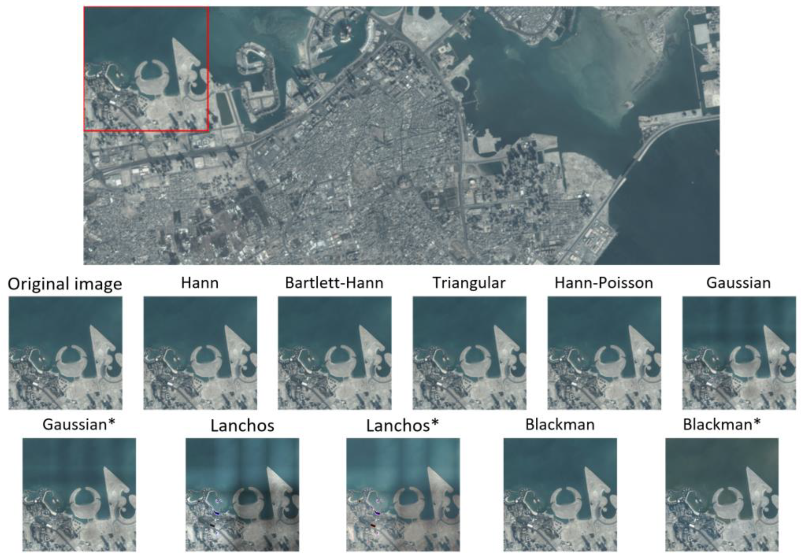
| Window Function\Metrics | MSE | RMSE | PSNR | UQI | SCC | SAM | SSIM | RASE | VIFP | NRMSE |
|---|---|---|---|---|---|---|---|---|---|---|
| Overlap | 0.00 | 0.00 | - | 1.00 | 1.00 | 0.00 | 1.00 | 0.00 | 1.00 | 0.00 |
| Hann a0 = 0.5 | 0.42 | 0.64 | 51.89 | 1.00 | 1.00 | 0.01 | 1.00 | 0.35 | 1.00 | 0.01 |
| Bartlett-Hann | 3.66 | 1.91 | 42.49 | 1.00 | 0.91 | 0.01 | 1.00 | 101.21 | 0.98 | 0.02 |
| Triangular | 3.84 | 1.95 | 42.29 | 1.00 | 0.90 | 0.01 | 1.00 | 104.21 | 0.98 | 0.02 |
| Hann-Poisson | 3.42 | 1.85 | 42.78 | 0.99 | 0.92 | 0.01 | 1.00 | 96.91 | 0.98 | 0.02 |
| Gaussian | 92.79 | 9.63 | 28.46 | 0.99 | 0.89 | 0.08 | 0.99 | 401.44 | 0.89 | 0.08 |
| Gaussian * | 75.74 | 8.70 | 29.34 | 1.00 | 0.88 | 0.07 | 0.99 | 354.06 | 0.87 | 0.07 |
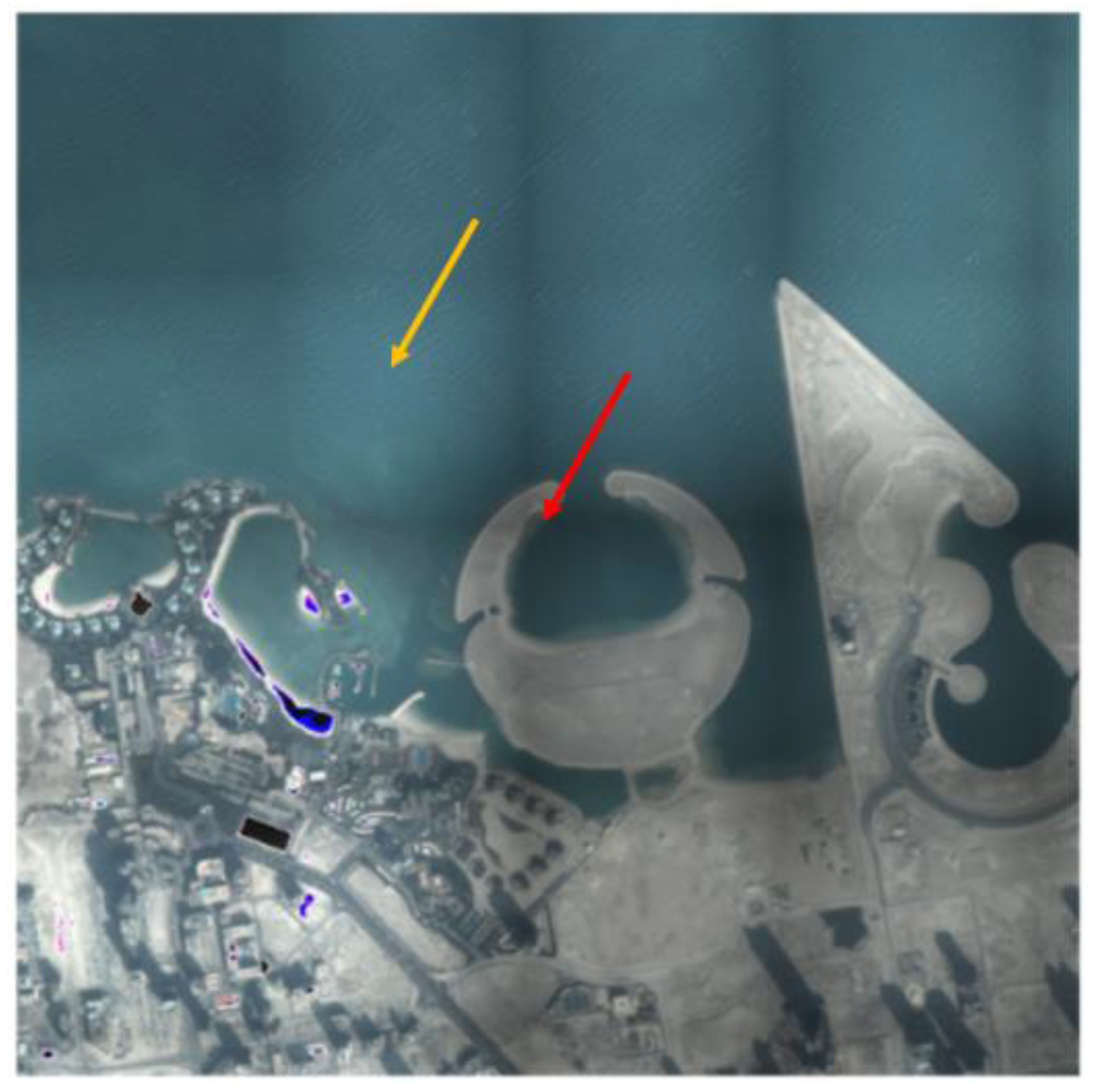
| Lanchos | 1288.29 | 35.89 | 17.03 | 0.90 | 0.85 | 0.30 | 0.88 | 1658.52 | 0.72 | 0.32 |
| Lanchos * | 863.22 | 29.38 | 18.77 | 0.95 | 0.81 | 0.24 | 0.88 | 1294.12 | 0.59 | 0.24 |
| Blackman | 16.68 | 4.08 | 35.91 | 1.00 | 0.90 | 0.02 | 1.00 | 207.04 | 0.97 | 0.03 |
| Blackman * | 3.23 | 1.80 | 43.03 | 1.00 | 0.89 | 0.01 | 1.00 | 87.88 | 0.97 | 0.01 |
| Iterations | Learning Rate |
|---|---|
| 35,000 | 2 × 10⁻⁴ |
| 80,000 | 1 × 10⁻⁴ |
| 80,000 | 5 × 10⁻⁵ |
| 100,000 | 2 × 10⁻⁵ |
Publisher’s Note: MDPI stays neutral with regard to jurisdictional claims in published maps and institutional affiliations. |
© 2022 by the authors. Licensee MDPI, Basel, Switzerland. This article is an open access article distributed under the terms and conditions of the Creative Commons Attribution (CC BY) license (https://creativecommons.org/licenses/by/4.0/).
Share and Cite
Karwowska, K.; Wierzbicki, D. Improving Spatial Resolution of Satellite Imagery Using Generative Adversarial Networks and Window Functions. Remote Sens. 2022, 14, 6285. https://doi.org/10.3390/rs14246285
Karwowska K, Wierzbicki D. Improving Spatial Resolution of Satellite Imagery Using Generative Adversarial Networks and Window Functions. Remote Sensing. 2022; 14(24):6285. https://doi.org/10.3390/rs14246285
Chicago/Turabian StyleKarwowska, Kinga, and Damian Wierzbicki. 2022. "Improving Spatial Resolution of Satellite Imagery Using Generative Adversarial Networks and Window Functions" Remote Sensing 14, no. 24: 6285. https://doi.org/10.3390/rs14246285