EMO-MVS: Error-Aware Multi-Scale Iterative Variable Optimizer for Efficient Multi-View Stereo

Abstract

Efficient dense reconstruction of objects or scenes has substantial practical implications, which can be applied to different 3D tasks (for example, robotics and autonomous driving). However, because of the expensive hardware required and the overall complexity of the all-around scenarios, efficient dense reconstruction using lightweight multi-view stereo methods has received much attention from researchers. The technological challenge of efficient dense reconstruction is maintaining low memory usage while rapidly and reliably acquiring depth maps. Most of the current efficient multi-view stereo (MVS) methods perform poorly in efficient dense reconstruction, this poor performance is mainly due to weak generalization performance and unrefined object edges in the depth maps. To this end, we propose EMO-MVS, which aims to accomplish multi-view stereo tasks with high efficiency, which means low-memory consumption, high accuracy, and excellent generalization performance. In detail, we first propose an iterative variable optimizer to accurately estimate depth changes. Then, we design a multi-level absorption unit that expands the receptive field, which efficiently generates an initial depth map. In addition, we propose an error-aware enhancement module, enhancing the initial depth map by optimizing the projection error between multiple views. We have conducted extensive experiments on challenging datasets Tanks and Temples and DTU, and also performed a complete visualization comparison on the BlenedMVS validation set (which contains many aerial scene images), achieving promising performance on all datasets. Among the lightweight MVS methods with low-memory consumption and fast inference speed, our F-score on the online Tanks and Temples intermediate benchmark is the highest, which shows that we have the best competitiveness in terms of balancing the performance and computational cost.

1. Introduction

Multi-view stereo (MVS) is one of the essential tasks in computer vision. It has long been studied by many researchers and has been widely applied in autonomous driving [1], virtual reality [2], robotics, and 3D reconstruction [3,4]. MVS is also capable of reconstructing ground terrain using aerial photography systems (such as satellites and drones). The core of the multi-view stereo task is to use stereo correspondence from multiple images as the main cue to reconstruct dense 3D representations. Currently, the reconstruction of 3D scenes is mainly based on the depth map method. However, the depth map acquisition is primarily divided into two-view and multi-view scenarios. The two-view scenarios are mainly used to obtain the disparity of corresponding pixels in the rectified image pairs by matching two adjacent views, and then calculating the depth [5]. However, obtaining the exact rectified image pairs for images with more varying viewpoints is difficult. In multi-view scenarios, multiple unrectified images can be used simultaneously, and depth estimation can be performed directly in depth space without the need to convert by calculating disparity. First, several hypothetical depth planes are proposed in the depth range. Then, the best depth plane is determined for each pixel by the dense correspondence between pixels of different views [6].

In detail, many conventional MVS methods [7,8,9,10] have yielded impressive results. Although hand-crafted operators can achieve high accuracy, the completeness of the constructed point cloud is affected by low-texture regions, illumination changes, and reflections, which make these methods usually unable to achieve a satisfactory quality of reconstruction in practical use. Many industrial applications require efficient algorithms, such as the real-time reconstruction of ground details by high-altitude sensors, UAV obstacle avoidance, and automatic driving of cars. Therefore, dense reconstruction with fast inference speed and low GPU memory has broad application prospects.

Recently, the popular learning-based methods [11,12,13,14,15,16,17] have significantly improved the overall reconstruction quality in challenging scenarios. MVSNet [11] is the first method that introduced deep learning technology to depth-map-based MVS tasks [18,19,20]. The subsequent learning-based MVS approaches emulate MVSNet [11] by constructing a 3D cost volume, regularizing it with a 3D CNN, and regressing the depth. Since 3D CNNs usually consume considerable time and GPU memory, some methods [21] downsample the input during feature extraction and compute the cost volume and depth map at low resolution. However, providing the depth map at low resolution may affect the accuracy since low-resolution depth maps lose much of the original information. Thus, the quality of the reconstructed point cloud is reduced.

To reduce memory consumption, some researchers have separated the memory requirements from the depth range and processed the cost volume sequentially at an additional runtime cost [14,22]. Apparently, increasing runtime for lower GPU memory consumption is not reasonable for efficient dense reconstruction. Another research direction [12,13] for the lightweight MVS method is to predict a high-resolution depth map from coarse to fine using a cascaded 3D cost volume. However, due to the limitation of 3D convolution, a satisfactory balance of overall reconstruction quality and computational complexity cannot be achieved. In summary, most learning-based MVS methods still experience high memory and computational costs when constructing and adjusting cost volumes, making it difficult to balance computational complexity and overall reconstruction quality.

To address the above problems, PatchmatchNet [23] and IterMVS [24] are proposed to solve the challenge of simultaneously maintaining low computational complexity and excellent overall quality. PatchmatchNet extends PatchMatch’s traditional propagation [5] and cost evaluation steps with adaptive aggregation, which improves accuracy and efficiency. Although PatchmatchNet has made significant progress, the F-scores on the Tanks and Temples benchmark and real-world applications show that its generalization performance is limited. IterMVS [24] retains PatchMatchNet’s initialization and uses the iterative structure of RAFT [25] in optical flow estimation. IterMVS [24] can achieve a better generalization performance while maintaining fast inference speed and low memory consumption and is the most advanced and efficient MVS method. However, these methods still have room for improvement.

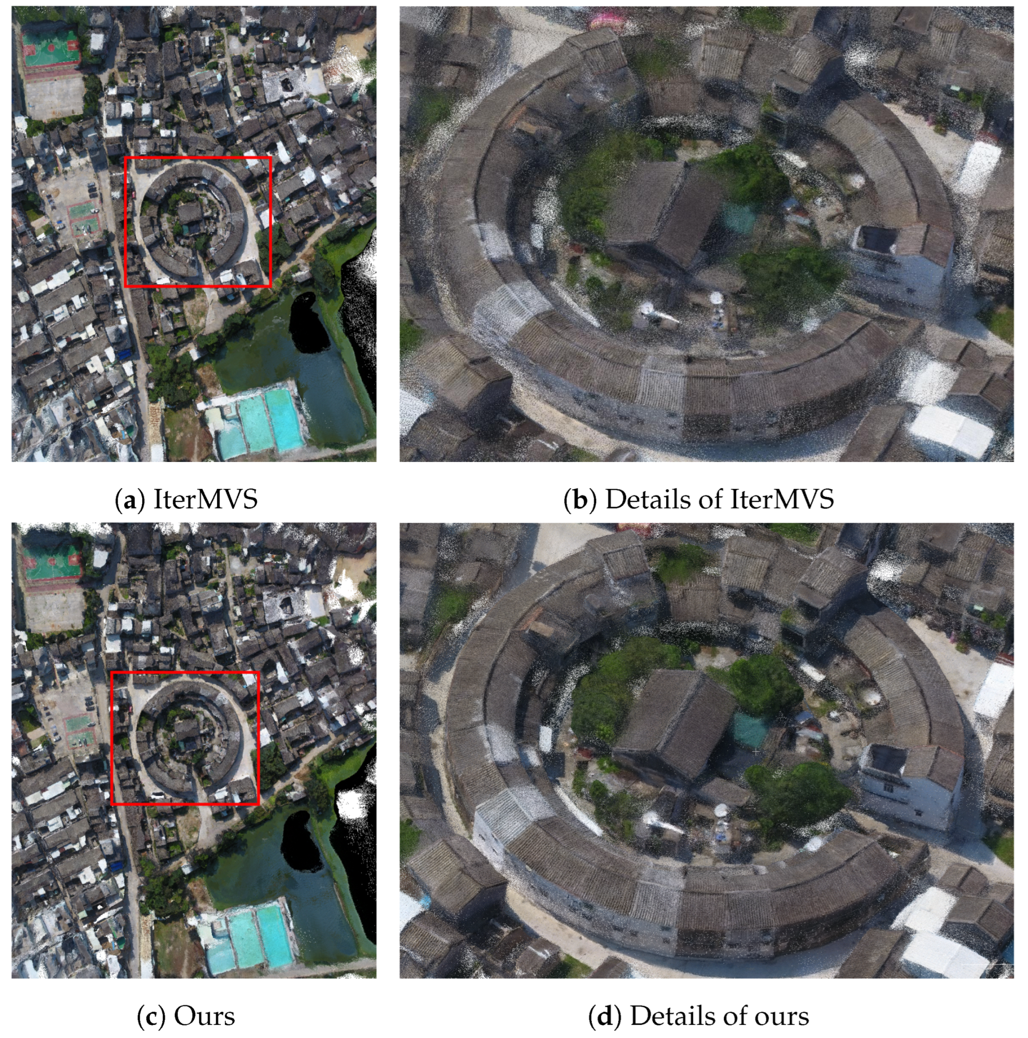
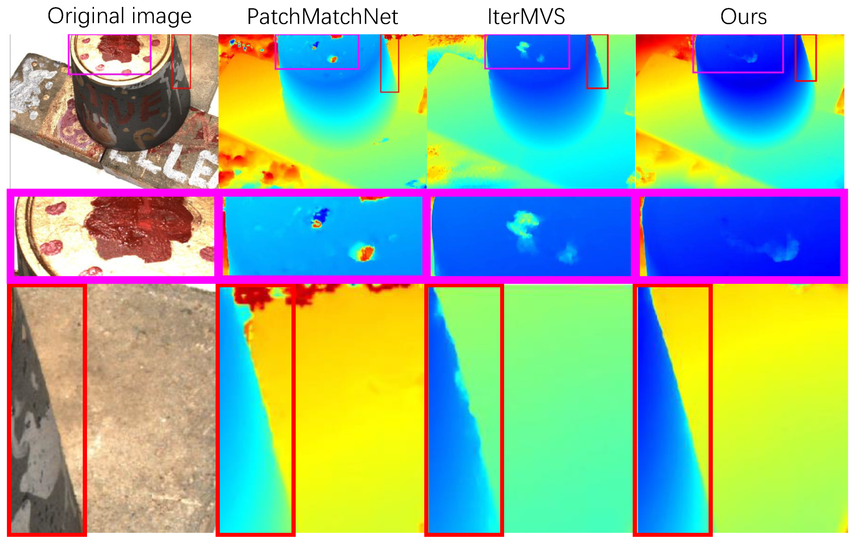
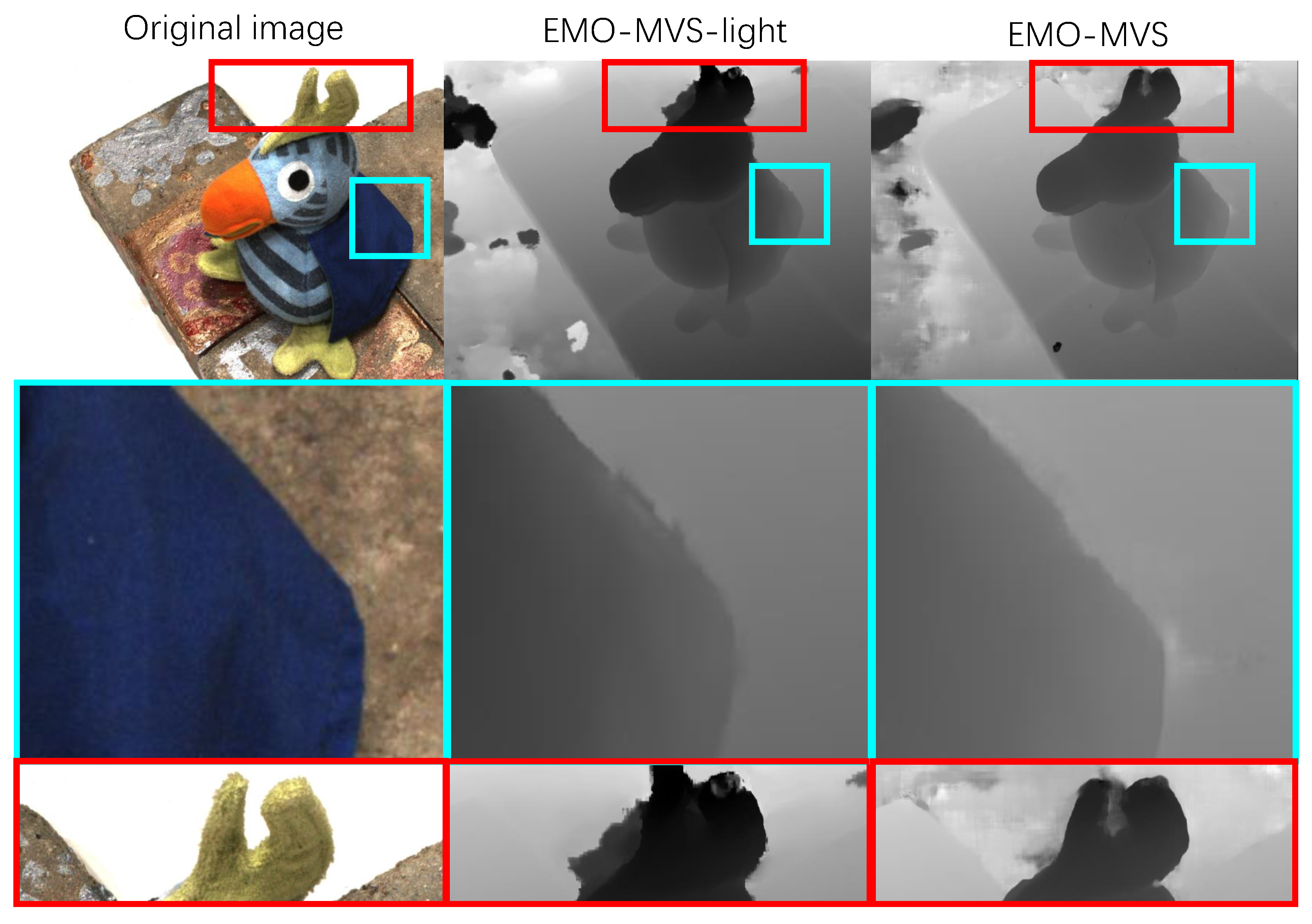
As shown in Figure 1, the details of the scene reconstructed by the existing efficient methods in the complex environment are not sufficiently satisfactory. Specifically, there are three important issues that have been overlooked. First, most efficient methods [23,26] rely too much on attention mechanisms, resulting in limited generalization performance. Second, many efficient approaches [21,23,24] only handle features at a single scale to lower the time complexity and space complexity. Thus, having only a small receptive field limits their ability to reconstruct details at weak and repetitive textures. Third, the efficient MVS methods [23,24] generate depth maps with unrefined target edges. When handling large-scale aerial images, this phenomenon is more obvious. The unrefined edges lead to more noise in the corresponding local point cloud, affecting the quality of the final reconstructed point cloud.

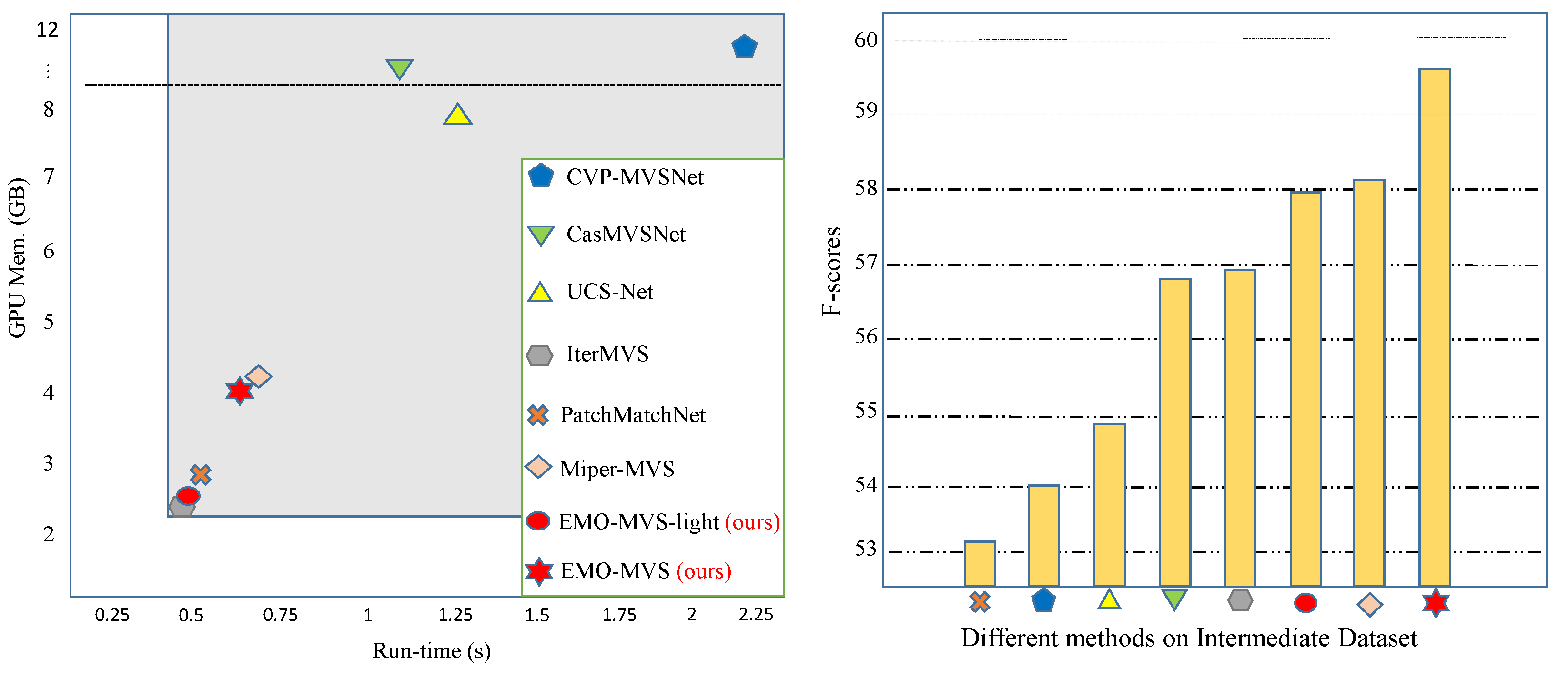
To address these three issues, we propose a high-efficiency multi-view stereo method named EMO-MVS that aims to significantly improve the generalization performance. Our comparison with current state-of-the-art methods is shown in Figure 2. In detail, EMO-MVS mainly includes three core components. First, we propose an iterative variable optimizer with a modified Conv-LSTM module as the core structure and optimize only the correction amount of the depth information in each iteration. Such a design allows for a more accurate perception of the amount of change in the depth information during depth optimization, thus enriching the depth hierarchy. Updating only the amount of variation instead of directly updating the depth map also better avoids overfitting. Second, modifications to the multilevel absorption unit are implemented with the aim of fusing the multiscale information in a more efficient and satisfactory manner. The updated module permits the expansion of the receptive field, which allows the network to retain its efficiency attributes. Third, we propose an error-aware enhancement module. The initial depth map is obtained by the first and second parts above, and then we project the source images with the initial depth map and calculate the projection error. After that, we optimize the projection error to obtain the residual depth, and the initial depth plus the residual depth is the final depth map. The experimental results show that EMO-MVS significantly improves the generalization performance and is more efficient than most of the previous MVS methods.

In summary, the contributions of this paper include the following:

• We propose a low-memory consumption, high-accuracy, and fast-inference-speed EMO-MVS framework for MVS tasks. The previous efficient MVS methods usually produce unrefined depth maps in large-scale aerial datasets, and EMO-MVS dramatically alleviates this problem.
• Specifically, we propose three core modules, including an iterative variable estimator that optimizes the depth variation, a multilevel absorption unit for efficient fusion of multiscale information, and an error-aware module that enhances the initial depth map.
• We validate our method’s effectiveness on the DTU and Tanks and Temples datasets. The results prove that our approach is the most competitive in terms of balancing performance and efficiency.

This paper is organized as follows. Section 2 introduces the current research status. Section 3 presents the proposed EMO-MVS model in detail. Section 4 conducts the experimental results and corresponding analysis. Section 5 summarizes our work.

2. Related Work

2.1. Conventional MVS

Conventional MVS methods have been widely used in many fields, such as robotics [27] and 3D maps [28]. Based on the scene representations, conventional MVS methods can be divided into three categories: voxel-based [29,30,31], point-based [7,32,33,34], and depth map-based [8,10,16,35,36,37]. Voxel-based methods estimate the relationship between each voxel and the surface, but they consume too much memory. Point-cloud-based methods directly process 3D points to densify the results iteratively, but the algorithm parallelism is not satisfactory. Depth map reconstruction methods use only one reference and a few source images for single depth map estimation. Point clouds can be generated by using depth map fusion, and the mesh can be reconstructed even further. Compared with the direct operation in three-dimensional space, this kind of mapping method from two-dimensional images to three-dimensional space has significant advantages in terms of flexibility and computational cost. However, although the conventional methods have achieved impressive results, they consume considerable computational resources and have limited effectiveness in complex scenarios.

2.2. Learning-Based MVS

Conventional methods have difficulties in estimating depth accurately in low-textured surfaces and under complex lighting environments. Recently, learning-based solutions [16] have addressed these issues and further enhanced the reconstruction quality. MVSNet [11] first proposes a differentiable homography and leverages the 3D cost volume in a learning pipeline; it also aggregates contextual information through a 3D convolutional network. However, its high computational cost and high memory consumption limit its ability to reconstruct large scenes. To construct an efficient and lightweight MVS pipeline, most researchers mainly prefer a cascade structure [13,38], which solves the MVS problem in a coarse-to-fine manner assuming decreasing depth hypotheses along the reference camera frustum at each stage. However, the cascade approaches have difficulties recovering details from errors introduced by coarse resolution. To this end, R-MVSNet and D2HC-MVSNet [14,22] use an RNN module to regularize the 2D cost maps along the depth direction, which is equivalent to sequentially processing the cost volume. This operation significantly reduces memory consumption but correspondingly greatly increases the runtime. Overall, devising approaches that simultaneously achieve fast inference speed, low memory consumption, and high overall reconstruction quality has always been a challenging problem. On the other hand, some methods [39,40] that ignore computational resource consumption and only emphasize performance have begun to consume increasing computational resources. However, the improvement in terms of accuracy and generalizability is not apparent. Since the performance improvement has encountered a bottleneck, it is currently more urgent to improve the running speed and memory utilization efficiency while maintaining high accuracy.

PatchmatchNet [23] extends the traditional propagation and cost evaluation steps in PatchMatch [5] with an adaptive aggregation method and achieves satisfactory results in terms of the balance between computational complexity and overall reconstruction quality. Although PatchmatchNet has made encouraging advancements, its generalization performance is still inadequate for some specific cases, which means that its application expansion in diverse real-world scenarios is also limited. IterMVS [24] takes advantages of PatchmatchNet and uses the iterative structure that has proven effective in stereo matching to achieve better generalization performance. However, a higher level of generalization performance is required in practical applications, especially when processing aerial photography images that contain large-scale scenes, which require a very excellent generalization performance.

Currently, the main reasons affecting the generalization performance of efficient MVS methods include overly simple information optimization processing mechanisms, small perceptual fields, and depth maps with unrefined target edges. In this paper, our iterative variable optimizer uses a modified Conv-LSTM structure with a strategy that optimizes the amount of depth variation reasonably and satisfactorily, and the multilevel absorption unit expands the receptive field with high computational efficiency. Therefore, our EMO-MVS generates depth maps with a more distinct depth hierarchy. On the other hand, the accuracy and completeness of the point cloud are significantly improved because our error-aware enhancement adequately combines the initial depth map, the projection error between views, and the original image with a large amount of high-frequency information.

3. Method

3.1. Overview

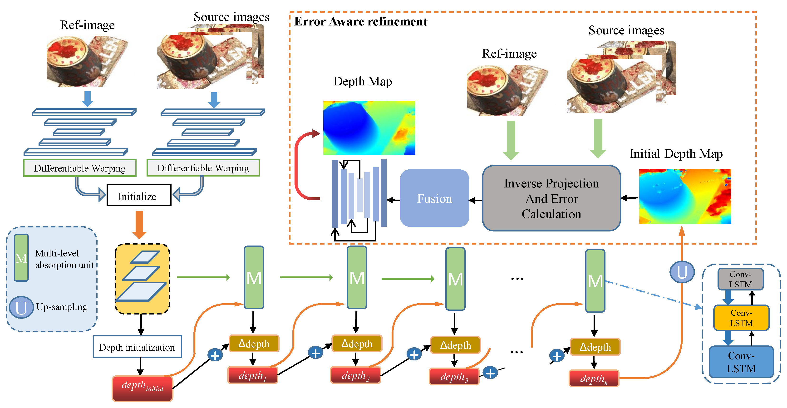
EMO-MVS estimates the depth maps from multiple overlapping RGB images. Specifically, our method accepts one reference image $I_0$ and N-1 source images ${\left\{I_i\right\}}_{i=1}^{N-1}$ as input and then obtains the depth map of the reference image. First, EMO-MVS constructs a correlation volume and an initial hidden state using the features extracted by FPN. Second, the above results are input into the first-order implicit optimizer at each iteration; this optimizer consists of our modified Conv-LSTM unit, which estimates information about the change in the depth values. In the first-order implicit optimizer, we also use a multilevel absorption unit to fuse the output states of the modified Conv-LSTM at three scales. After optimization, the initial depth map is obtained. Finally, the initial depth map is enhanced by optimizing the pixel error of the geometric projection transformation to obtain the final depth map. Our main structure is shown in Figure 3.

3.2. Feature Extractor and Initialization

Feature Extractor: The FPN (Feature Pyramid Network) has been proven to have excellent feature extraction results in many visual tasks. Given N input images of size W × H, we adopt $I_0$ and ${\left\{I_i\right\}}_{i=1}^{N-1}$ to denote the reference image and the source images. Then, we adopt a feature pyramid network (FPN) for feature extraction of the input reference image and the source images. The feature extraction module generates feature maps at three scales $F_l$, where $l=1,2,3$, and the channel is $16,32,64$, respectively.

Correlation Volume: To find the dense correspondence between different views, we use the extracted features for de-homogenization [11], following most learning-based MVS methods, we warp the source features into front-to-parallel planes. Specifically, for a pixel p in the reference view and the j-th depth hypothesis, $d_j$:=$d_j\left(p\right)$ with known intrinsic ${\left\{K\right\}}_{i=0}^{N-1}$ and relative transformations ${\left\{R_{0,i}\right|T_{0,i}\}}_{i=1}^{N-1}$ between reference view 0 and source view i, we can compute the corresponding pixel $p_{i,j}$:=$p_i\left(d_j\right)$ in the source view as:

$$p_{i,j}=K_i.(R_{0.i}.(K_0^{-1}.p.d_j)+T_{0,i}),$$

(1)

After de-homogenization, we obtain the feature $F_i$ of the source image in the reference image coordinate frame, and we use $F_i$ and $F_0$ (which are features of the reference image) to calculate the correlation volume and matching similarity [23,24].

Initialization: To initialize the hidden state h of Conv-LSTM, before the iterative update, we use the previously-obtained matching similarity and correlation volume to generate the initial hidden state H and $dept{h}_{initial}$ [23,24], which are the inputs to the iterative variable optimizer.

3.3. Iterative Variable Optimizer

In other related fields that utilize 3D vision, iterative structures have proven to be quite effective methods [25,41], and most approaches use the GRU as their iterative update unit. However, in our research, Conv-LSTM cells with a finer gate structure have better performance. The GRU-based optimizer has only one hidden state h transfer between iterations, while the LSTM-based optimizer has two (h and C). Since the updated matrix of the depth map is coupled with the hidden state h, introducing an extra hidden state C to decouple the update matrix and the hidden state h can retain more effective semantic information across iterations.

To obtain a strong Conv-LSTM cell, our main improvements to the current Conv-LSTM are as follows: (1) We use a fusion head to simultaneously receive multiscale or single-scale information as needed. This approach allows us to use multiscale information more flexibly when passing through the subsequent multilevel absorbing units. (2) We use dilated convolutions instead of regular convolutions to obtain a larger receptive field, which helps recover challenging details. (3) By removing the bias from the original Conv-LSTM, we avoid redundant computation. Our modified Conv-LSTM is also comparable to the GRU in terms of efficiency.

In detail, we input the initialized hidden state H into our modified Conv-LSTM module, and our Conv-LSTM is as follows:

$$Xlist=Cat\left([x_1\dots \dots x_n]\right),$$

(2)

$$f_k=\sigma \left(DilateCon{v}_f([h_{k-1},Xlis{t}_k],W_f)\right),$$

(3)

$$i_k=\sigma \left(DilateCon{v}_i([h_{k-1},Xlis{t}_k],W_i)\right),$$

(4)

$$g_k=tanh\left(\sigma \left(DilateCon{v}_g([h_{k-1},Xlis{t}_k],W_g)\right)\right),$$

(5)

$$C_k=C_{k-1}\odot f_k+i_k\odot g_k,$$

(6)

$$o_k=\sigma \left(DilateCon{v}_o([h_{k-1},Xlis{t}_k],W_o)\right),$$

(7)

$$h_k=o_k\odot tanh\left(C_k\right),$$

(8)

where $\sigma$ is the sigmoid nonlinearity, and ⊙ is the Hadamard product. The subscript $k(k=0\dots \dots K)$ denotes the index of iterations, $h_k$ and $C_k$ are the outputs of the $k-th$ iteration of our Conv-LSTM module, and the correlation volume and the matching similarity are integrated to obtain $x_n$. To simultaneously receive single-scale or multiscale information, we aggregate the input information as follows: $Xlist=Cat\left([x_1\dots \dots x_n]\right)$.

In addition, each update of our Conv-LSTM hidden state only contains information about the depth change amount rather than the entire depth map. This design avoids the overfitting that may occur as the number of iterations increases. Our final hidden state $h_k^{final}$ for depth prediction at each iteration is calculated as follows:

$$h_i^{final}=\sum _{i=1}^k{h}_i.$$

(9)

We utilize the output $h_k^{final}$ of the iterative variable optimizer for probability regression and depth prediction [24] to obtain the depth map $dept{h}_k$ of the k-th iteration.

3.4. Multi-Level Absorption Unit

To achieve low memory consumption and high efficiency, some efficient approaches, such as [24,26], often only incorporate feature information from single-scale processing for subsequent depth estimation. A broader receptive field in the MVS task enables the network to deliver more precise depth estimations in areas with poor texture details. The most direct way to expand the receptive field is to use a multiscale fusion strategy. Nonetheless, multiscale strategies usually incur high computational costs, which affect inference speed and memory usage more significantly. Accordingly, we design an accurate and efficient multilevel absorption unit (MAU) that expands the receptive field by interactively absorbing low-scale information through a high-scale Conv-LSTM. MAU effectively balances accuracy, speed, and memory usage.

Specifically, we downsample the initialized hidden states to obtain the medium-scale and low-scale hidden states. We also widen our iterative structure to handle the other two scales of hidden states. In the update stage of multiscale information, the lowest resolution modified Conv-LSTM units are fused across scales by introducing features of medium resolution. These medium-resolution modified Conv-LSTM units are fused by introducing features of low and high resolution, and the highest-resolution units are fused by introducing features of both medium and low resolution.

The multiscale fusion mechanism is as the following formulas:

$$\begin{array}{cc}\hfill & C_l^k,h_l^k=CLSTMCell(C_l^{k-1},h_l^{k-1},ctx,pool\left(h_m^{k-1}\right)),\hfill \end{array}$$

(10)

$$\begin{array}{cc}\hfill & C_m^k,h_m^k=CLSTMCell(C_m^{k-1},h_m^{k-1},ctx,pool\left(h_h^{k-1}\right),interp\left(h_l^{k-1}\right)),\hfill \end{array}$$

(11)

$$\begin{array}{cc}\hfill & C_h^k,h_h^k=CLSTMCell(C_l^{k-1},h_l^{k-1},ctx,dept{h}_{k-1},interp\left(h_m^{k-1}\right),interp\left(h_l^{k-1}\right)),\hfill \end{array}$$

(12)

$$\begin{array}{cc}\hfill & FinalOutput=h_h^k,\hfill \end{array}$$

(13)

where l, m, and h denote low, middle, and high resolution, respectively. $CLSTMCell$ is our modified Conv-LSTM module, and $pool$ and $interp$ denote the downsampling and upsampling methods, respectively. k is the number of iterations, and $ctx$ is the integration of the correlation volume and matching similarity. The input to each iteration of our process uses the output of the previous iteration. For the highest resolution, the module not only makes use of upsampled middle and low resolution but also accepts the depth map of the $(k-1)th$ iteration as input.

A multilevel absorption unit (MAU) can effectively fuse information from multiple scales due to the cross-pollination of information between hidden states at multiple scales, and most of the low- and middle-scale information is absorbed by the high-scale hidden states. On the one hand, since we only output the highest-scale information at the end, the inference speed and memory usage is almost the same as that when using only single-scale information. On the other hand, since we avoid the computational cost of multiscale information fusion for the final output, our computational cost is smaller than that of the common multiscale fusion method. Therefore, our method is faster than the common multiscale update module.

3.5. The Structure of Error-Aware Enhancement

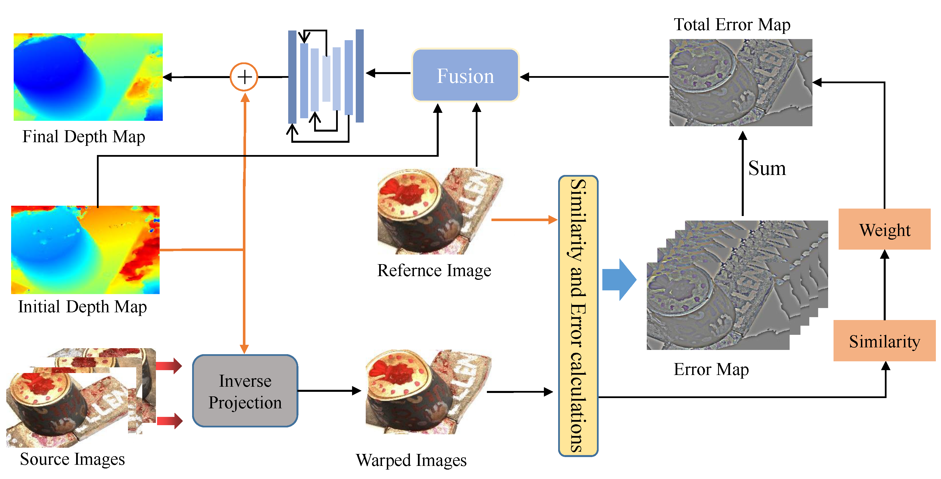
Depth maps with unrefined target edges can result in anomalous noise in the final point cloud during the depth map fusion step [42,43]. The filtering process based on geometric restrictions can remove a significant portion of the apparent noise, but it still retains noise near the edge of the target point clouds. Therefore, to improve the accuracy and completeness of the final point cloud, it is necessary to enhance the initial depth map generated by the efficient MVS method. Therefore, we propose error-aware enhancement with the structure shown in Figure 4.

First, by using inverse-project wrapping, the reconstructed source image can be calculated using the reference image and the initial depth estimate. Then, subtraction is performed to obtain the error map. Finally, the error map, reference image, and initial depth map are fused and input into the hourglass network, and the refined depth map is calculated.

3.5.1. Inverse Projection and Error Calculation

To convert the error of the inaccurate initial depth ($D_{initial}$) into a projection error, we project the source images $I_i$ into the coordinate system of the reference image $I_0$ by using the initial depth. Then, we calculate the projection error by using the difference between the reference image and the new source image produced by the projection. The mathematical formula is as follows:

$$p_i^{\prime }=(R_i{R}_0^{-1}(d\left(p\right)K_0^{-1}-T_0)+T_i)K_i,i=\{1.\dots \dots N-1\},$$

(14)

where {$K_0$,$K_i$}, {$R_0$,$R_i$}, {$T_0$,$T_i$} denote the cameras intrinsic rotations and translations of the reference image and source images, respectively. A point on the reference image is represented by p, and the new point that p warps to on the source image is indicated by $p_i^{\prime }$. The depth value predicted by point p on the initial depth map is denoted by the notation d(p).

After obtaining the mapping point $p_i^{\prime }$, we utilize $G_i$($p_i^{\prime }$) to represent the grayscale value of $p_i^{\prime }$. The grayscale error between point p and point $p_i^{\prime }$ is then available to us and is calculated as follows:

$$Error=G_i\left(p_i^{\prime }\right)-G_0\left(p\right),$$

(15)

$$ErrorMap=G_i-G_0,$$

(16)

where $G_i$ and $G_0$ are the grayscale representations of source image $I_i$ and reference image $I_0$, respectively. After obtaining the grayscale error $Error$ of a single pixel, we use $ErrorMap$ to represent the projected error map between the source image $I_i$ and the reference image $I_0$.

To measure the error between all views, we need to calculate the total projection error for all views, which is obtained by weighting the sum of $ErrorMap$ for all views. We call it the total error map, and it is denoted by $Tmap$. The mathematical formula is as follows:

$$Tmap=\sum _{i=1}^{N-1}{W}_i(G_i-G_0),$$

(17)

Since the source images from different angles have different target overlap areas relative to the reference image, the weight of each error map in the core error map should also be different. We propose a simplified version of the two-view matching similarity $S_i$ [23,44,45] for calculating the weight $W_i$ as follows:

$$S_i={〈G_i.G_0〉}^r+{〈G_i.G_0〉}^g+{〈G_i.G_0〉}^b,$$

(18)

$$W_i=\frac{S_i}{{\sum }_{j=1}^{N-1}{S}_j},$$

(19)

where r,g,b denote the three channels of the original image, and $\langle .\rangle$ denotes the dot product.

3.5.2. Information Fusion and Optimization

To further enhance the details of the initial depth map $D_{initial}$, we introduce the rich high-frequency features in the reference image $I_0$ and then fuse this feature information with the initial depth map $D_{initial}$ and the total error map $Tmap$ as follows:

$$Fusion=Cat(Con{v}_1\left(Cat(Tmap,I_0)\right),Con{v}_2\left(D_{initial}\right)).$$

(20)

Finally, we use the hourglass optimizer to optimize the fusion result $Fusion$ to obtain the depth residual map $D_{residuals}$, and the final result of the depth map D is computed as follows:

$$D_{residuals}=Hourglass\left(Fusion\right),$$

(21)

$$D=D_{initial}+D_{residuals},$$

(22)

Overall, we apply the projection relationship of geometric mapping between multiple views to the learning-based optimization module, which incurs small computational costs while improving the accuracy. In addition, weighting the projection error of each image in accordance with the variations is implemented through diverse shooting angles, which improves the generalization performance of our module for various scenarios.

4. Experiments

4.1. Datasets

We tested our experiment on three public datasets. DTU [46] is an indoor dataset under laboratory conditions that contains 124 scenes with 49 views and 7 illumination conditions. We adopted the same training, validation, and evaluation split as defined in [47]. DTU can effectively verify the MVS data fitting ability. BlendedMVS [48] is a large-scale synthetic dataset that contains 106 training scans and 7 validation scans. Tanks and Temples [49] is a public benchmark that provides realistic video sequences divided into intermediate and more challenging advanced sets. This division makes the MVS task practical for validating the generalization of deep learning methods.

4.2. Implementation Details

To demonstrate the proposed method’s high efficiency, we compare the lightweight methods without error-aware enhancement to EMO-MVS-light, which is slightly more efficient than the full version of EMO-MVS. Following common practice [40,50], EMO-MVS is first trained on the DTU training set and evaluated on the DTU test set; then, it is fine-tuned on BlendedMVS before being tested on the Tanks and Temples benchmark. We adopt a resolution of $640\times 512$ for the input images and set the view number parameter to $N=5$ for training on DTU. In the BlendedMVS dataset, we adopt a resolution of $768\times 576$ for the input images and set the view number parameter to $N=5$ for the training process. In all of the experiments, to balance computational complexity and overall reconstruction quality, the number of iterations K is set to 4 during the training stage. In addition, we use Adam [51] as our optimizer. The learning rate is initially set to 0.001 and is halved every four epochs. We train a total of 20 epochs, and the batch size is 4 on DTU and 2 on the BlendedMVS dataset. Our models are trained on a single Nvidia Tesla V100 GPU. Finally, we predict a depth map for each reference image and fuse the predicted depth map into the point cloud. We adopt the same parameters for depth map fusion and the same loss function as in [24].

4.3. Main Results on DTU Dataset

4.3.1. Effect Verification on DTU

We compare conventional and learning-based methods, where learning-based methods are classified as emphasizing accuracy or efficiency. We set the number of input views to 5 and the resolution to 1160 × 1152. The quantitative results on the DTU evaluation set are summarized in

Table 1. Quantitative results of reconstruction quality on the DTU evaluation dataset (↓). A and B are the conventional methods and high-accuracy learning-based methods, respectively. C and D are high-efficiency learning-based methods. Bold font represents the best.

	Method	Acc.	Comp.	Overrall
A	Tola	0.342	1.190	0.766
	Gipuma	0.283	0.873	0.578
B	MVSNet	0.396	0.527	0.462
	R-MVSNet	0.383	0.452	0.417
	CIDER	0.417	0.437	0.427
	P-MVSNet	0.406	0.434	0.420
	CasMVSNet	0.325	0.385	0.355
	$D^2$HC-RMVSNet	0.395	0.378	0.386
	CVP-MVSNet	0.296	0.406	0.351
	AA-RMVSNet	0.376	0.339	0.357
	Vis-MVSNet	0.369	0.361	0.365
	EPP-MVSNet	0.413	0.296	0.355
C	Fast-MVSNet	0.336	0.403	0.370
	PatchMatchNet	0.427	0.277	0.352
	IterMVS	0.373	0.354	0.363
D	EMO-MVS-light (ours)	0.372	0.345	0.358
	EMO-MVS (ours)	0.360	0.328	0.344

, which indicates the excellent performance of our method. Although Gipuma [8] leads in accuracy and PatchmatchNet [23] achieves completeness, the overall performance (the average of accuracy and completeness) of our method is significantly stronger than both.

Our depth map estimation for a reflective sample is shown in Figure 5; it demonstrates that our method is barely disturbed by reflections and that we have better edge effects. Our point reconstruction for a low-textured sample is shown in Figure 6. The red boxes reflect the higher accuracy of our method for weak textures, and the colors of the reconstructed point clouds are closer to the ground truth. In addition, the blue box reflects the higher completeness of our point cloud in the areas where the structured light camera does not provide ground truth.

4.3.2. Efficiency Verification on DTU

The core of the high-efficiency MVS method is to maintain fast inference speed and low memory consumption without reducing overall reconstruction quality as much as possible. All tests were performed on an RTX2080ti GPU. Our experiments compare the inference speed and memory usage of various methods under the same environmental conditions. As shown in

Table 2. Comparison of memory consumption and runtime on DTU evaluation dataset (↓) [46]. Bold font represents the best.

Method	Input Size	Memory (GB)	Time (s)	Acc. (mm)	Comp. (mm)	Overall (mm)
UCS-Net	1600 × 1184	7.76	0.964	0.340	0.349	0.345
CVP-MVSNet	1600 × 1200	9.86	1.912	0.296	0.406	0.351
CasMVSNet	1600 × 1200	9.58	0.796	0.325	0.385	0.355
Fast-MVSNet	1600 × 1200	6.05	0.642	0.331	0.401	0.366
PatchmatchNet	1600 × 1200	2.68	0.345	0.427	0.277	0.352
IterMVS	1600 × 1152	2.26	0.278	0.373	0.354	0.363
EMO-MVS-light(ours)	1600 × 1152	2.24	0.281	0.372	0.345	0.358
EMO-MVS(ours)	1600 × 1152	3.83	0.446	0.360	0.328	0.344

, our lightweight approach achieves excellent overall results while maintaining excellent inference speed and the lowest memory consumption.

Furthermore, our full version obtains the best overall results but still maintains efficient runtime and memory consumption levels. Compared to UCSNet [52], our runtime and memory consumption are less than half of those of UCSNet, which indicates that our error-aware enhancement significantly enhances the initial depth map while incurring a small computational cost.

4.4. Main Results on the Tanks and Temples Dataset

Since the Tanks and Temples [49] dataset has many complex outdoor scenes and variable lighting environments, the validation results on this dataset can fully reflect the generalization performance of learning-based MVS methods. As with most methods, we set the number of input views to 7 and the resolution to 1920 × 1080. The camera parameters and depth ranges are estimated with OpenMVG [53], and the corresponding quantitative results on both the intermediate and advanced sets are reported in

Table 3. Quantitative results of different methods on the Tanks and Temples benchmark. ’Mean’ refers to the mean F-score of all scenes (↑). Bold font represents the best.

	Intermediate Dataset									Advanced Dataset
F-Score	Fam.	Franc.	Horse	Light.	M60	Pan.	Play.	Train	Mean	Audi.	Ballr.	Courtr.	Museum	Palace	Temple	Mean
OpenMVS	71.69	51.12	42.76	58.98	54.72	56.17	59.77	45.69	55.11	24.49	37.39	38.21	47.48	27.25	31.79	34.43
MVSNet	55.99	28.55	25.07	50.79	53.96	50.86	47.90	34.69	43.48	-	-	-	-	-	-	-
R-MVSNet	69.96	46.65	32.59	42.95	51.88	48.80	52.00	42.38	48.40	12.55	29.09	25.06	38.68	19.14	24.96	24.91
CIDER	56.79	32.39	29.89	54.67	53.46	53.51	50.48	42.85	46.76	12.77	24.94	25.01	33.64	19.18	23.15	23.12
Point-MVSNet	61.79	41.15	34.20	50.79	51.97	50.85	52.38	43.06	48.27	-	-	-	-	-	-	-
CasMVSNet	76.37	58.45	46.26	55.81	56.11	54.06	58.18	49.51	56.84	19.81	38.46	29.10	43.87	27.36	28.11	31.12
UCS-Net	76.09	53.16	43.03	54.00	55.60	51.49	57.38	47.89	54.83	-	-	-	-	-	-	-
CVP-MVSNet	76.50	47.74	36.34	55.12	57.28	54.28	57.43	47.54	54.03	-	-	-	-	-	-	-
D2HC-RMVSNet	74.69	56.04	49.42	60.08	59.81	59.61	60.04	53.92	59.20	-	-	-	-	-	-	-
Fast-MVSNet	65.18	39.59	34.98	47.81	49.16	46.20	53.27	42.91	47.39	-	-	-	-	-	-	-
PatchMatchNet	66.99	52.64	43.24	54.87	52.87	49.54	54.21	50.81	53.15	23.69	37.73	30.04	41.80	28.31	32.29	32.31
MVSTR	76.92	59.82	50.16	56.73	56.53	51.22	56.58	47.48	56.93	22.83	39.04	33.87	45.46	27.95	27.97	32.85
PatchMatch-RL	60.37	43.26	36.43	56.27	57.30	53.43	59.85	47.61	51.81	24.28	40.25	35.87	44.13	22.43	23.73	31.78
RayMVSNet	78.56	61.96	45.48	57.58	61.01	59.76	59.20	52.32	59.49	-	-	-	-	-	-	-
IterMVS	76.12	55.80	50.53	56.05	57.68	52.62	55.70	50.99	56.94	25.90	38.41	31.16	44.83	29.59	35.15	34.17
EMO-MVS-light (ours)	76.07	55.09	51.81	56.10	60.23	56.27	54.33	53.35	57.91	25.88	38.90	31.94	44.48	29.94	36.72	34.65
EMO-MVS (ours)	77.85	59.69	54.73	57.69	58.62	56.40	56.19	54.88	59.51	24.42	40.71	33.62	46.40	30.38	38.35	35.65

. Compared to IterMVS [24], our lightweight method is significantly better (from 56.94 to 57.91) in terms of generalization performance, and it benefits from our highly accurate iterative variable optimizer and efficient fusion strategy with its enlarged receptive field.

In addition, the full version of our method even surpasses the latest nonefficient method, RayMVSNet [54], in terms of generalization performance while still maintaining fast inference speed and low memory consumption. We report a depth map comparison in a large and complex outdoor scene, as shown in Figure 7. Our approach has sharper edges for most objects and is more robust in terms of depth estimation for small objects, which are susceptible to interference. Our depth map is also more explicit at the stone pillars and stairs, which shows that our method can handle repeated textures better. Such obvious advantages show that the error-aware enhancement fully exploits and optimizes the projection error, significantly improving the generalization performance.

4.5. Ablation Study

4.5.1. Core Modules

We conduct an extensive ablation study to validate the enhancements that the proposed modules contribute. Here, we use the DTU training set to train our method, and all tests were performed on the DTU evaluation set, as shown in

Table 4. Ablation Study on DTU dataset [46] (↓). Our baseline consists of the depth initialization in Figure 3, followed by a single-scale GRU iterative optimization operator. Bold font represents the best.

NO.	Baseline	Iterative Variable Optimizer	Multi-Level Absorption	Error-Aware	Acc.	Comp.	Overall
1	√				0.373	0.354	0.363
2		√			0.369	0.352	0.360
3		√	√		0.370	0.347	0.358
4		√	√	√	0.360	0.328	0.344

.

We can summarize the following conclusions: First, compared with No. 1 and No. 2, the iterative variable optimizer significantly improves precision and completeness compared to the baseline, which shows the effectiveness of the iterative variable optimizer. Second, compared with No. 3 and No. 4, a single-scale strategy, multi-level absorbing units improve the completeness of reconstruction while maintaining similar accuracy, which indicates that expanding the receptive field can better restore the details at weak textures, thus making up for the integrity of the point cloud. Finally, compared with No. 4 and No. 5, we report the effect with and without the error-aware enhancement module, which shows the validity of the error-aware enhancement module.

4.5.2. Comparison of Details

Multi-level absorption unit and Common multiscale fusion unit: To demonstrate the excellent performance and fast-inference-speed of the multilevel absorption unit solution, we compare it with the common multiscale solutions. The results are shown in

Table 5. Comparison of two multi-scale fusion approaches on DTU [46] dataset (↓).

Method	Acc. (mm)	Comp. (mm)	Overall (mm)	Runtime (s)
Common multiscale fusion	0.380	0.339	0.359	0.412
Multi-level absorption unit	0.370	0.347	0.358	0.281

, and our efficiency improves by 30% compared to common multiscale fusion. The common multiscale scheme has a slight advantage in terms of completeness, but our overall performance is still better. To be fair, the $Fusion$ module of the common multiscale approach uses only a simple 2D convolution, and the mathematical formula is as follows:

$$\begin{array}{cc}\hfill & C_l^k,h_l^k=CLSTMCell(C_l^{k-1},h_l^{k-1},ctx),\hfill \end{array}$$

(23)

$$\begin{array}{cc}\hfill & C_m^k,h_m^k=CLSTMCell(C_m^{k-1},h_m^{k-1},ctx),\hfill \end{array}$$

(24)

$$\begin{array}{cc}\hfill & C_h^k,h_h^k=CLSTMCell(C_l^{k-1},h_l^{k-1},ctx),\hfill \end{array}$$

(25)

$$\begin{array}{cc}\hfill & FinalOutput=Fusion(h_l^k,h_m^k,h_h^k).\hfill \end{array}$$

(26)

Before the error-aware enhancement, the reconstruction accuracy mainly depends on the accuracy of the highest-scale Conv-LSTM update unit for updating the depth change amount. The reconstruction’s better completeness depends on incorporating more low-scale information in the optimized output. Incorporating more low-scale information means better perceptual field expansion and, thus, better performance in weak textured regions. We think the reason for the lack of satisfactory completeness is that before the error-aware enhancement, the reconstruction accuracy mainly depends on the accuracy of the highest-scale Conv-LSTM update unit for updating the depth change amount. The reconstruction’s better completeness depends on incorporating more low-scale information in the optimized output. Incorporating more low-scale information means better perceptual field expansion and, thus, better performance in weak textured regions.

The method for generating the total error map: For the error-aware enhancement, we note that different ways of computing the total error map can produce significantly different results, especially for the generalization performance. In our experimental comparison, we consider the DTU dataset, where all environments are indoor scenes, and the Tanks and Temples dataset, which contains complex outdoor scenes. The results are shown in

Table 6. Comparison of two ways to calculate the total error map.

Method	DTU (↓)			Tanks and Temples (↑)
	Acc. (mm)	Comp. (mm)	Overall (mm)	F-Score (Mean)
Summation	0.361	0.332	0.346	58.80
Weighted Summation	0.360	0.328	0.344	59.51

. The weighted summation shows a slight improvement in the overall metric on the DTU dataset, and it contributes a significant improvement on the Tanks and Temples dataset. We speculate that this result is due to the complex lighting in the outdoor scene and the matching interference of other outdoor objects (e.g., buildings, tree branches), which differ in each view. Therefore, the error map generated by each source view should have a different impact on the final total error map.

Comparison of depth estimates using the aerial photography dataset: To demonstrate the advantages of our method in high-altitude aerial scenes, we compare the depth maps with IterMVS [24] on the BlendedMVS [48] validation set. To demonstrate the generalization performance of our method, all methods are trained only on the DTU dataset. The results are shown in Figure 8. Our method has a better depth hierarchy due to the larger perceptual field obtained by the multiscale strategy, and because it benefits from optimizing the projection error with the error-aware module, our depth map has sharper object edges.

Comparison with and without error-aware enhancement: To reflect the effect of enhancement, we compare EMO-MVS and EMO-MVS-light (without enhancement) by visualizing scan4 in DTU. As shown in Figure 9, EMO-MVS is more robust to edge depth estimation, while some parts are more susceptible to matching interference. In addition, EMO-MVS produces a depth map with more sharpened edges in all details. These results reflect the outstanding contribution of enhancement to improving the edge effect.

5. Conclusions

In this paper, to balance between accuracy and efficiency, we propose a novel MVS method, EMO-MVS. First, we use an RNN-based iterative structure to estimate the update matrix of depth in each iteration and accumulates to get the depth map. In the process, to expand the receptive field while maintaining high efficiency, we adopt an absorbing multiscale fusion strategy where the final hidden state is only output at the highest scale to increase inference speed and save memory consumption. In addition, we adopt the perceptual projection error method to refine the depth map, which dramatically improves the performance at a lower computational cost. Our error-aware enhancement module can be easily integrated into other existing MVS frameworks. Finally, the experimental results prove that our method is the most competitive one among the current low-memory and high-efficiency methods. In the future, we plan to explore the integration of our modules into stereo matching or other related fields.

References

1. Yurtsever, E.; Lambert, J.; Carballo, A.; Takeda, K. A survey of autonomous driving: Common practices and emerging technologies. IEEE Access 2020, 8, 58443–58469. [Google Scholar] [CrossRef]
2. Burdea, G.C.; Coiffet, P. Virtual Reality Technology; John Wiley & Sons: Hoboken, NJ, USA, 2003. [Google Scholar]
3. Garcia, E.; Jimenez, M.A.; De Santos, P.G.; Armada, M. The evolution of robotics research. IEEE Robot. Autom. Mag. 2007, 14, 90–103. [Google Scholar] [CrossRef]
4. Geiger, A.; Ziegler, J.; Stiller, C. Stereoscan: Dense 3d reconstruction in real-time. In Proceedings of the 2011 IEEE Intelligent Vehicles Symposium (IV), Baden-Baden, Germany, 5–9 June 2011; pp. 963–968. [Google Scholar]
5. Bleyer, M.; Rhemann, C.; Rother, C. Patchmatch Stereo-Stereo Matching with Slanted Support Windows. In Proceedings of the British Machine Vision Conference, Vienna, Austria, 29 August–2 September 2011; Volume 11, pp. 1–11. [Google Scholar]
6. Baillard, C.; Zisserman, A. A plane-sweep strategy for the 3D reconstruction of buildings from multiple images. Int. Arch. Photogramm. Remote Sens. 2000, 33, 56–62. [Google Scholar]
7. Furukawa, Y.; Ponce, J. Accurate, dense, and robust multiview stereopsis. IEEE Trans. Pattern Anal. Mach. Intell. 2009, 32, 1362–1376. [Google Scholar] [CrossRef] [PubMed]
8. Galliani, S.; Lasinger, K.; Schindler, K. Massively parallel multiview stereopsis by surface normal diffusion. In Proceedings of the IEEE International Conference on Computer Vision, Santiago, Chile, 7–13 December 2015; pp. 873–881. [Google Scholar]
9. Schonberger, J.L.; Frahm, J.M. Structure-from-motion revisited. In Proceedings of the IEEE Conference on Computer Vision and Pattern Recognition, Las Vegas, NV, USA, 26 June–1 July 2016; pp. 4104–4113. [Google Scholar]
10. Xu, Q.; Tao, W. Multi-scale geometric consistency guided multi-view stereo. In Proceedings of the IEEE/CVF Conference on Computer Vision and Pattern Recognition, Long Beach, CA, USA, 15–20 June 2019; pp. 5483–5492. [Google Scholar]
11. Yao, Y.; Luo, Z.; Li, S.; Fang, T.; Quan, L. Mvsnet: Depth inference for unstructured multi-view stereo. In Proceedings of the European Conference on Computer Vision (ECCV), Munich, Germany, 8–14 September 2018; pp. 767–783. [Google Scholar]
12. Gu, X.; Fan, Z.; Zhu, S.; Dai, Z.; Tan, F.; Tan, P. Cascade cost volume for high-resolution multi-view stereo and stereo matching. In Proceedings of the IEEE/CVF Conference on Computer Vision and Pattern Recognition, Online, 14–19 June 2020; pp. 2495–2504. [Google Scholar]
13. Yang, J.; Mao, W.; Alvarez, J.M.; Liu, M. Cost volume pyramid based depth inference for multi-view stereo. In Proceedings of the IEEE/CVF Conference on Computer Vision and Pattern Recognition, Online, 13–19 June 2020; pp. 4877–4886. [Google Scholar]
14. Yao, Y.; Luo, Z.; Li, S.; Shen, T.; Fang, T.; Quan, L. Recurrent mvsnet for high-resolution multi-view stereo depth inference. In Proceedings of the IEEE/CVF Conference on Computer Vision and Pattern Recognition, Long Beach, CA, USA, 15–20 June 2019; pp. 5525–5534. [Google Scholar]
15. Ma, X.; Gong, Y.; Wang, Q.; Huang, J.; Chen, L.; Yu, F. EPP-MVSNet: Epipolar-assembling based Depth Prediction for Multi-view Stereo. In Proceedings of the IEEE/CVF International Conference on Computer Vision, Online, 11–17 October 2021; pp. 5732–5740. [Google Scholar]
16. Stathopoulou, E.K.; Battisti, R.; Cernea, D.; Remondino, F.; Georgopoulos, A. Semantically derived geometric constraints for MVS reconstruction of textureless areas. Remote Sens. 2021, 13, 1053. [Google Scholar] [CrossRef]
17. Wang, Q.; Liu, X.; Liu, W.; Liu, A.A.; Liu, W.; Mei, T. Metasearch: Incremental product search via deep meta-learning. IEEE Trans. Image Process. 2020, 29, 7549–7564. [Google Scholar] [CrossRef]
18. Lipson, L.; Teed, Z.; Deng, J. Raft-stereo: Multilevel recurrent field transforms for stereo matching. In Proceedings of the 2021 International Conference on 3D Vision (3DV), Online, 1–3 December 2021; pp. 218–227. [Google Scholar]
19. Xu, H.; Zhang, J. Aanet: Adaptive aggregation network for efficient stereo matching. In Proceedings of the IEEE/CVF Conference on Computer Vision and Pattern Recognition, Online, 13–19 June 2020; pp. 1959–1968. [Google Scholar]
20. Chang, J.R.; Chen, Y.S. Pyramid stereo matching network. In Proceedings of the IEEE Conference on Computer Vision and Pattern Recognition, Salt Lake City, UT, USA, 18–22 June 2018; pp. 5410–5418. [Google Scholar]
21. Yu, Z.; Gao, S. Fast-mvsnet: Sparse-to-dense multi-view stereo with learned propagation and gauss-newton refinement. In Proceedings of the IEEE/CVF Conference on Computer Vision and Pattern Recognition, Online, 18–22 June 2020; pp. 1949–1958. [Google Scholar]
22. Yan, J.; Wei, Z.; Yi, H.; Ding, M.; Zhang, R.; Chen, Y.; Wang, G.; Tai, Y.W. Dense hybrid recurrent multi-view stereo net with dynamic consistency checking. In Proceedings of the European Conference on Computer Vision, Glasgow, UK, 23–28 August 2020; Springer: Berlin/Heidelberg, Germany, 2020; pp. 674–689. [Google Scholar]
23. Wang, F.; Galliani, S.; Vogel, C.; Speciale, P.; Pollefeys, M. Patchmatchnet: Learned multi-view patchmatch stereo. In Proceedings of the IEEE/CVF Conference on Computer Vision and Pattern Recognition, Online, 19–25 June 2021; pp. 14194–14203. [Google Scholar]
24. Wang, F.; Galliani, S.; Vogel, C.; Pollefeys, M. IterMVS: Iterative Probability Estimation for Efficient Multi-View Stereo. In Proceedings of the IEEE/CVF Conference on Computer Vision and Pattern Recognition, New Orleans, LA, USA, 19–20 June 2022; pp. 8606–8615. [Google Scholar]
25. Teed, Z.; Deng, J. Raft: Recurrent all-pairs field transforms for optical flow. In Proceedings of the European Conference on Computer Vision, Glasgow, UK, 23–28 August 2020; Springer: Berlin/Heidelberg, Germany, 2020; pp. 402–419. [Google Scholar]
26. Yang, Z.; Ren, Z.; Shan, Q.; Huang, Q. Mvs2d: Efficient multi-view stereo via attention-driven 2d convolutions. In Proceedings of the IEEE/CVF Conference on Computer Vision and Pattern Recognition, New Orleans, LA, USA, 19–20 June 2022; pp. 8574–8584. [Google Scholar]
27. Tanduo, B.; Martino, A.; Balletti, C.; Guerra, F. New Tools for Urban Analysis: A SLAM-Based Research in Venice. Remote Sens. 2022, 14, 4325. [Google Scholar] [CrossRef]
28. Zhou, G.; Wang, Q.; Huang, Y.; Tian, J.; Li, H.; Wang, Y. True2 Orthoimage Map Generation. Remote Sens. 2022, 14, 4396. [Google Scholar] [CrossRef]
29. Kutulakos, K.N.; Seitz, S.M. A theory of shape by space carving. In Proceedings of the Seventh IEEE International Conference on Computer Vision, Kerkyra, Greece, 20–25 September 1999; Volume 1, pp. 307–314. [Google Scholar]
30. Seitz, S.M.; Dyer, C.R. Photorealistic scene reconstruction by voxel coloring. Int. J. Comput. Vis. 1999, 35, 151–173. [Google Scholar] [CrossRef]
31. Ulusoy, A.O.; Black, M.J.; Geiger, A. Semantic multi-view stereo: Jointly estimating objects and voxels. In Proceedings of the 2017 IEEE Conference on Computer Vision and Pattern Recognition (CVPR), Honolulu, HI, USA, 21–26 July 2017; pp. 4531–4540. [Google Scholar]
32. Lhuillier, M.; Quan, L. A quasi-dense approach to surface reconstruction from uncalibrated images. IEEE Trans. Pattern Anal. Mach. Intell. 2005, 27, 418–433. [Google Scholar] [CrossRef] [PubMed] [Green Version]
33. Gonçalves, G.; Gonçalves, D.; Gómez-Gutiérrez, Á.; Andriolo, U.; Pérez-Alvárez, J.A. 3D reconstruction of coastal cliffs from fixed-wing and multi-rotor uas: Impact of sfm-mvs processing parameters, image redundancy and acquisition geometry. Remote Sens. 2021, 13, 1222. [Google Scholar] [CrossRef]
34. Wang, F.; Yang, J.F.; Wang, M.Y.; Jia, C.Y.; Shi, X.X.; Hao, G.F.; Yang, G.F. Graph attention convolutional neural network model for chemical poisoning of honey bees’ prediction. Sci. Bull. 2020, 65, 1184–1191. [Google Scholar] [CrossRef]
35. Campbell, N.D.; Vogiatzis, G.; Hernández, C.; Cipolla, R. Using multiple hypotheses to improve depth-maps for multi-view stereo. In Proceedings of the European Conference on Computer Vision, Marseille, France, 12–18 October 2008; Springer: Berlin/Heidelberg, Germany, 2008; pp. 766–779. [Google Scholar]
36. Schönberger, J.L.; Zheng, E.; Frahm, J.M.; Pollefeys, M. Pixelwise view selection for unstructured multi-view stereo. In Proceedings of the European Conference on Computer Vision, Amsterdam, The Netherlands, 11–14 October 2016; Springer: Berlin/Heidelberg, Germany, 2016; pp. 501–518. [Google Scholar]
37. Zhou, L.; Zhang, Z.; Jiang, H.; Sun, H.; Bao, H.; Zhang, G. DP-MVS: Detail Preserving Multi-View Surface Reconstruction of Large-Scale Scenes. Remote Sens. 2021, 13, 4569. [Google Scholar] [CrossRef]
38. Zhang, J.; Yao, Y.; Li, S.; Luo, Z.; Fang, T. Visibility-aware multi-view stereo network. arXiv 2020, arXiv:2008.07928. [Google Scholar]
39. Wei, Z.; Zhu, Q.; Min, C.; Chen, Y.; Wang, G. Aa-rmvsnet: Adaptive aggregation recurrent multi-view stereo network. In Proceedings of the IEEE/CVF International Conference on Computer Vision, Montreal, QC, Canada, 10–17 October 2021; pp. 6187–6196. [Google Scholar]
40. Ding, Y.; Yuan, W.; Zhu, Q.; Zhang, H.; Liu, X.; Wang, Y.; Liu, X. Transmvsnet: Global context-aware multi-view stereo network with transformers. In Proceedings of the IEEE/CVF Conference on Computer Vision and Pattern Recognition, New Orleans, LA, USA, 21–24 June 2022; pp. 8585–8594. [Google Scholar]
41. Gu, X.; Yuan, W.; Dai, Z.; Tang, C.; Zhu, S.; Tan, P. Dro: Deep recurrent optimizer for structure-from-motion. arXiv 2021, arXiv:2103.13201. [Google Scholar]
42. Dai, A.; Nießner, M.; Zollhöfer, M.; Izadi, S.; Theobalt, C. Bundlefusion: Real-time globally consistent 3d reconstruction using on-the-fly surface reintegration. ACM Trans. Graph. (ToG) 2017, 36, 1. [Google Scholar] [CrossRef]
43. Izadi, S.; Kim, D.; Hilliges, O.; Molyneaux, D.; Newcombe, R.; Kohli, P.; Shotton, J.; Hodges, S.; Freeman, D.; Davison, A.; et al. KinectFusion: Real-time 3D reconstruction and interaction using a moving depth camera. In Proceedings of the 24th Annual ACM Symposium on User Interface Software and Technology, Santa Barbara, CA, USA, 16–19 October 2011; pp. 559–568. [Google Scholar]
44. Xu, Q.; Tao, W. Pvsnet: Pixelwise visibility-aware multi-view stereo network. arXiv 2020, arXiv:2007.07714. [Google Scholar]
45. Guo, X.; Yang, K.; Yang, W.; Wang, X.; Li, H. Group-wise correlation stereo network. In Proceedings of the IEEE/CVF Conference on Computer Vision and Pattern Recognition, Long Beach, CA, USA, 16–20 June 2019; pp. 3273–3282. [Google Scholar]
46. Aanæs, H.; Jensen, R.R.; Vogiatzis, G.; Tola, E.; Dahl, A.B. Large-scale data for multiple-view stereopsis. Int. J. Comput. Vis. 2016, 120, 153–168. [Google Scholar] [CrossRef] [Green Version]
47. Ji, M.; Gall, J.; Zheng, H.; Liu, Y.; Fang, L. Surfacenet: An end-to-end 3d neural network for multiview stereopsis. In Proceedings of the IEEE International Conference on Computer Vision, Venice, Italy, 22–29 October 2017; pp. 2307–2315. [Google Scholar]
48. Yao, Y.; Luo, Z.; Li, S.; Zhang, J.; Ren, Y.; Zhou, L.; Fang, T.; Quan, L. Blendedmvs: A large-scale dataset for generalized multi-view stereo networks. In Proceedings of the IEEE/CVF Conference on Computer Vision and Pattern Recognition, Nashville, TN, USA, 20–25 June 2020; pp. 1790–1799. [Google Scholar]
49. Knapitsch, A.; Park, J.; Zhou, Q.Y.; Koltun, V. Tanks and temples: Benchmarking large-scale scene reconstruction. ACM Trans. Graph. (ToG) 2017, 36, 1–13. [Google Scholar] [CrossRef]
50. Peng, R.; Wang, R.; Wang, Z.; Lai, Y.; Wang, R. Rethinking Depth Estimation for Multi-View Stereo: A Unified Representation and Focal Loss. arXiv 2022, arXiv:2201.01501. [Google Scholar]
51. Hartmann, W.; Galliani, S.; Havlena, M.; Van Gool, L.; Schindler, K. Learned multi-patch similarity. In Proceedings of the IEEE International Conference on Computer Vision, Venice, Italy, 22–29 October 2017; pp. 1586–1594. [Google Scholar]
52. Cheng, S.; Xu, Z.; Zhu, S.; Li, Z.; Li, L.E.; Ramamoorthi, R.; Su, H. Deep stereo using adaptive thin volume representation with uncertainty awareness. In Proceedings of the IEEE/CVF Conference on Computer Vision and Pattern Recognition, Seattle, WA, USA, 13–19 June 2020; pp. 2524–2534. [Google Scholar]
53. Moulon, P.; Monasse, P.; Perrot, R.; Marlet, R. Openmvg: Open multiple view geometry. In International Workshop on Reproducible Research in Pattern Recognition; Springer: Berlin/Heidelberg, Germany, 2016; pp. 60–74. [Google Scholar]
54. Xi, J.; Shi, Y.; Wang, Y.; Guo, Y.; Xu, K. RayMVSNet: Learning Ray-based 1D Implicit Fields for Accurate Multi-View Stereo. In Proceedings of the IEEE/CVF Conference on Computer Vision and Pattern Recognition, New Orleans, LA, USA, 21–24 June 2022; pp. 8595–8605. [Google Scholar]
Figure 1. Comparison of point clouds on the BlendedMVS validation set. The scene is generated from aerial images captured by drones, and the IterMVS [24] point cloud is unrefined in terms of details such as eaves, while our point cloud is more explicit.
Remotesensing 14 06085 g001
Figure 2. Comparison with the state-of-the-art learning-based MVS methods on Tanks and Temples. The left graph shows the GPU memory and run-time of various methods (image size 1920 × 1024, 7 views). The right graph is the comparison of the F-score (↑). Where EMO-MVS-light is the version without Error-Aware enhancement, EMO-MVS is our full version, our approach has the best balance between computational costs and F-score.
Remotesensing 14 06085 g002
Figure 3. EMO-MVS architecture. EMO-MVS first extracts features via an FPN. Then, the initialization depth ( d e p t h i n i t i a l ) is obtained by using the initialization module, and the iterative variable optimizer optimizes the initialization depth ( d e p t h i n i t i a l ). Inside the iterative variable optimizer, we use multilevel absorption units to aggregate the multiscale information, and after several optimization iterations, we obtain the initial depth map. Finally, we input the initial depth map into our error-aware enhancement module to obtain the final depth map.
Remotesensing 14 06085 g003
Figure 4. Error-Aware enhancement.
Remotesensing 14 06085 g004
Figure 5. Depth estimation of scan1 on DTU. Our method has a clear advantage in reflections and edges, as shown in the red boxes.
Remotesensing 14 06085 g005
Figure 6. Point reconstruction of scan13 on DTU evaluation dataset.
Remotesensing 14 06085 g006
Figure 7. Depth estimation of Temple on Tanks and Temples [49].
Remotesensing 14 06085 g007
Figure 8. Comparison of depth estimation on the BlendedMVS validation set. Our depth map is significantly finer than IterMVS [24] in terms of target edge effect and depth level.
Remotesensing 14 06085 g008
Figure 9. Comparison with and without Error-Aware enhancement.
Remotesensing 14 06085 g009