Article

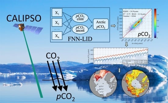
Carbon Air–Sea Flux in the Arctic Ocean from CALIPSO from 2007 to 2020

1
Southern Marine Science and Engineering Guangdong Laboratory (Guangzhou), No. 1119, Haibin Rd., Nansha District, Guangzhou 511458, China
2
State Key Laboratory of Satellite Ocean Environment Dynamics, Second Institute of Oceanography, Ministry of Natural Resources, Hangzhou 310012, China
3
State Key Laboratory of Tropical Oceanography, South China Sea Institute of Oceanology, Chinese Academy of Sciences, Guangzhou 510301, China
*
Author to whom correspondence should be addressed.
Remote Sens. 2022, 14(24), 6196; https://doi.org/10.3390/rs14246196
Submission received: 27 October 2022 / Revised: 2 December 2022 / Accepted: 4 December 2022 / Published: 7 December 2022
(This article belongs to the Special Issue Oceanographic Lidar in the Study of Marine Systems)

Abstract

:
Quantified research on the Arctic Ocean carbon system is poorly understood, limited by the scarce available data. Measuring the associated phytoplankton responses to air–sea CO2 fluxes is challenging using traditional satellite passive ocean color measurements due to low solar elevation angles. We constructed a feedforward neural network light detection and ranging (LiDAR; FNN-LID) method to assess the Arctic diurnal partial pressure of carbon dioxide (pCO2) and formed a dataset of long-time-series variations in diurnal air–sea CO2 fluxes from 2001 to 2020; this study represents the first time spaceborne LiDAR data were employed in research on the Arctic air–sea carbon cycle, thus providing enlarged data coverage and diurnal pCO2 variations. Although some models replace Arctic winter Chl-a with the climatological average or interpolated Chl-a values, applying these statistical Chl-a values results in potential errors in the gap-filled wintertime pCO2 maps. The CALIPSO measurements obtained through active LiDAR sensing are not limited by solar radiation and can thus provide ‘fill-in’ data in the late autumn to early spring seasons, when ocean color sensors cannot record data; thus, we constructed the first complete record of polar pCO2. We obtained Arctic FFN-LID-fitted in situ measurements with an overall mean R2 of 0.75 and an average RMSE of 24.59 µatm and filled the wintertime observational gaps, thereby indicating that surface water pCO2 is higher in winter than in summer. The Arctic Ocean net CO2 sink has seasonal sources from some continental shelves. The growth rate of Arctic seawater pCO2 is becoming larger and more remarkable in sectors with significant sea ice retreat. The combination of sea surface partial pressure and wind speed impacts the diurnal carbon air–sea flux variability, which results in important differences between the Pacific and Atlantic Arctic Ocean. Our results show that the diurnal carbon sink is larger than the nocturnal carbon sink in the Atlantic Arctic Ocean, while the diurnal carbon sink is smaller than the nocturnal carbon sink in the Pacific Arctic Ocean.

Graphical Abstract

1. Introduction

The ocean is a vital sink for anthropogenic CO2 and absorbed approximately 30% of our emissions between the beginning of the industrial revolution and the 1950s [1]. Currently, due to the lack of available data, there is a demand to assess the entire annual cycle of the partial pressure of carbon dioxide (pCO2) variabilities as a solution for understanding the onset and evolution of oceanic acidification [2]. For the modern ocean, the annual variations in pCO2 and related variables are generally well understood with nonthermal effects dominating in the subpolar regions, whereas the temperature-driven variations dominate the subtropics [3,4]. Sea surface pCO2 is increasing at a rate roughly equivalent to the increase in atmospheric CO2 in almost all parts of the global ocean [5,6,7]. However, recent global ocean carbon estimates still hide substantial interannual and regional fluctuations. Quantified research is needed, especially in regions with scarce available data, such as the Arctic Ocean (north of 65°N) and marginal seas, as these areas were excluded from many previous global surveys due to their limited data coverage [8,9,10].
The Arctic Ocean is changing in many aspects, with decreasing sea ice cover and increasing pCO2 being among the fastest-changing factors [11] (Intergovernmental Panel on Climate Change (IPCC), 2014). Over the past 3 decades, climate warming has induced remarkable changes in the Arctic ocean–ice–atmosphere system: increased sea ice losses [12,13], altered surface circulation [14,15,16], freshened surface water [17,18] and enhanced primary production [19]. In addition, ocean acidification is most pronounced in the Arctic, as CO2 solubility increases at cold temperatures and a lower total alkalinity causes systems to become more sensitive to anthropogenic CO2 [20,21]. Early observations indicated that the Arctic Ocean is a strong CO2 sink with persistently low pCO2 values in the highly productive slope and shelf regions [22], while more recent studies have suggested that rapid air–sea gas exchanges and warming have led to high pCO2 values approaching atmospheric CO2 concentrations [23,24]; however, these studies were based on limited observations and thus may have been affected by uneven spatiotemporal coverage. Thus, the pCO2 trends in the Arctic Ocean are poorly understood due to observational limitations and the added complexity of sea ice melt [25].
Arctic air–sea carbon flux measurements have been performed from ships for more than 30 decades by measuring the difference in the partial pressure of CO2 within the surface ocean and the atmosphere [26,27,28]. In addition, eddy covariance methods have often been used in recent years, thus providing an independent estimate of sea-to-air fluxes [29,30]. However, measured observations are rare and expensive in the Arctic due to the presence of complex environments, such as frequent high-intensity storms and low winter temperatures. The key source of uncertainty is the lack of data from this remote region, as few long-term monitoring programs and experiments have been performed; only Alaska and parts of Canada and Scandinavia (Greenland) are better represented [31]. Arrigo et al., 2006 found the annual mean pCO2 was 313 ± 4.1 μatm before 2003 in Greenland [32]. Benefiting from the increasing density of in situ measurements of sea surface CO2 fugacity and massive amounts of remote sensing data, a multitude of sea surface pCO2 reconstruction methods based on data interpolation approaches or machine learning have emerged [8]. Different artificial neural networks have succeeded in filling temporal and spatial data gaps [33,34,35,36,37,38,39,40,41]. However, passive remote sensing data quality is poor in Polar Regions and the coverage area is very limited, resulting in errors occurring in Antarctica or the Arctic among previous studies. Moreover, solar radiation-driven passive radiometers are greatly affected by polar night, resulting in large amounts of missing ocean color observations in the high-latitude region throughout wintertime, such as Chl-a measurements and their derivative pCO2 products. For example, chlorophyll-a concentrations, which are usually used to describe productivity, can be confounded by the presence of sea ice, clouds and solar radiation loss [26,39].
Recent advanced observations, such as spaceborne light detection and ranging (LiDAR) data, are filling these critical data needs. Lu et al., 2014 provided global Chl-a and particulate organic carbon concentrations and Behrenfeld et al., 2017 measured the annual cycles of phytoplankton biomass in polar regions [42,43]. A high-resolution LiDAR dataset containing both diurnal and nocturnal measurements (taken at approximately 13:40 and 01:40 local time, respectively), has also recently been employed to develop a retrieval approach for diurnal Chl-a and wind speed data. Hu estimated the wind speed and wave slope variance at the global scale and found that high-spatial-resolution (70-m) wind data from the CloudSat and Cloud-Aerosol Lidar and Infrared Pathfinder Satellite Observation (CALIPSO) platform can help reduce uncertainties in air–sea exchanges [44,45]. Compared to traditional satellite ocean color remote sensing, LiDAR measurements provide new measurements of ocean phytoplankton properties at both daytime and nighttime, including in polar regions, thus improving our understanding of Arctic phytoplankton primary productivity and carbon fluxes [46,47,48,49].
In Section 2, we described and introduced the datasets we used in this study, including the methods of diurnal chlorophyll-a concentration (Chl-a) and wind speed retrieval from the Cloud-Aerosol Lidar with Orthogonal Polarization (CALIOP) and the preprocessing of observation data and other remote sensing environmental data. Then, in Section 3 and Section 4, we compared the retrieved feedforward neural network-LiDAR (FNN-LID) pCO2 with the observations, estimated the long-time-series variations in the surface pCO2 and C-flux in the Arctic Ocean and analyzed the climatological diurnal variations. Finally, in Section 5, we summarized the developed approach and the main results achieved and provided recommendations for future biogeochemical studies using active LiDAR remote sensing measurements.

2. Materials and Methods
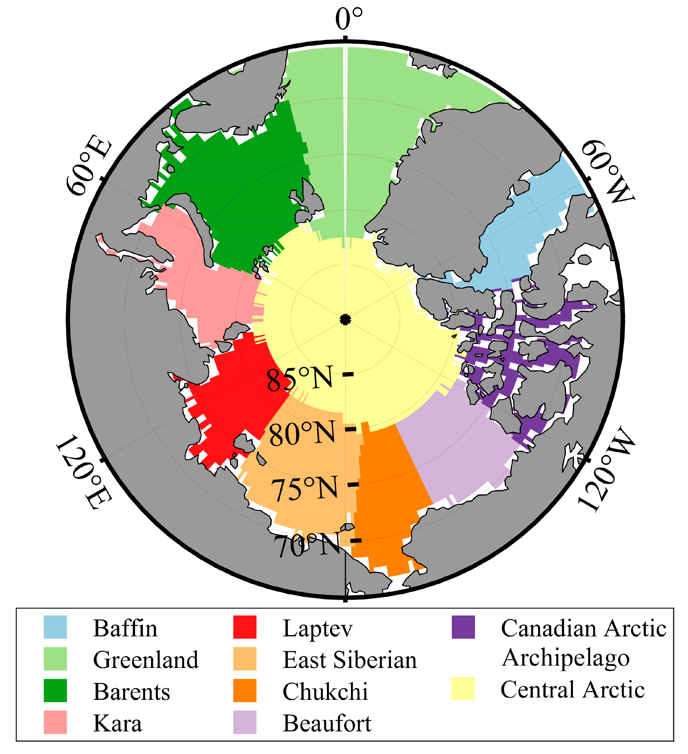
2.1. Arctic Sectors

The Arctic was divided into 10 sectors: Baffin Bay, Greenland Sea, Barents Sea, Kara Sea, Laptev Sea, East Siberian Sea, Chukchi Sea, Beaufort Sea, Canadian Arctic Archipelago and central Arctic Ocean. These subregions were then delineated using a region mask provided by the National Snow and Ice Data Center (NSIDC, available online: https://masie_web.apps.nsidc.org/pub/DATASETS/NOAA/G02135/seaice_analysis/ (accessed on 11 September 2022)); this mask has been used in many Arctic studies and consists of 3912 pixels per scene in the polar stereographic projection centered on the North Pole. We selected the high latitudes north of 60°N and regridded the mask to a spatial resolution of 1 × 1° (Figure 1).

2.2. Data

2.2.1. Observations

The Surface Ocean CO2 Atlas (SOCAT) (available online: http://www.socat.info/ (accessed on 20 August 2022)) community provides a key dataset of gridded monthly CO2 fugacity (fCO2) with data available since 2011 [50,51]. The latest SOCAT version, SOCATv2022, contains 33.7 million quality-controlled fCO2 observations from moorings, ships and drifters recorded over the period from 1957 to 2022 with an accuracy better than 5 μatm [52], including 2,534,512 observations in the Arctic (Figure 2). The gridded fCO2 estimates were converted to pCO2 values using the following formulation (see, e.g., [53]):
p CO 2 = f CO 2 exp p B + 2 δ R T 1 ,
where p CO 2 and f CO 2 are in microatmospheres (µatm), p is the total atmospheric surface pressure (in Pa), B and δ are viral coefficients [54], R is the gas constant and T is the absolute temperature.
The Global Ocean Data Analysis Project (GLODAP) v2.2020 is a synthesis effort agglomerating chemical water analysis data from more than 1.2 million water samples collected on 946 global cruises [55,56]. The GLODAP dataset encompasses 135,389 quality-controlled and normalized chemical water measurements in the Arctic, providing 29,305 discrete fCO2 values over 42 years of scientific exploration, and we used the coastal East Siberian data from GLOADP as a complementary (Figure 2).
Figure 2. The distributions of in situ fCO2 from SOCATv2022 and GLODAPv2.2020 in the Arctic Ocean. The observations of pCO2 including all the SOCAT data (north of 65°N) and the coastal East Siberian data from GLOADP as a complementary.
Remotesensing 14 06196 g002

2.2.2. CALIPSO Datasets

We used the active remote sensing data developed by the National Aeronautics and Space Administration (NASA) (available online: http://orca.science.oregonstate.edu/lidar_nature_2019.php (accessed on 19 August 2022)), including CALIPSO Level-1B V4.10 data products, Aerosol, LiDAR Level-2 Cloud and Merged Layer V4.20 products [57,58]. The CALIOP LiDAR is an active sensor producing simultaneous laser pulses with dual polarization at 532 nm, and the measured signal is corrected for after-pulse and polarization-crosstalk effects before being processed [59]. After correcting the influences of transient crosstalk and response, b b p was calculated from the vertical-parallel ratio [60,61,62], and Chl-a was estimated using the following formula [43]:
b b p   532 2 K d   β w + 0.32   0.98 2     1 2 K d   β w + 0.32   0.98 2   ,
Chl - a = log 0.17 b b p 2.0 × 10 4 ,
where β w + is the subsurface column-integrated backscatter of the perpendicular component, K d   is the diffuse attenuation coefficient at 532 nm (where K d is 1.76, see Behrenfeld et al., 2017; 2019) and δ p is the particulate depolarization ratio. Hence, Chl-a can be estimated based on the relational formula of b b p .
To validate the Chl-a results, we compared the global Chl-a values in the regions where ocean observations are available throughout the year from both CALIOP and the Moderate Resolution Imagining Spectrometer (MODIS) passive ocean color sensor. The MODIS data used in this study are Level-3 products with a spatial resolution of 9 km (available online: http://oceancolor.gsfc.nasa.gov (accessed on 16 July 2022)). At the global scale, we found excellent agreement (north r2 = 0.75, n = 12,775, p < 0.001) between the Chl-a values from the two sensors, thus lending confidence to the CALIOP retrievals (Figure 3A). In the polar zones, however, CALIOP continued to characterize Chl-a distributions right up to the ice edge throughout the extended periods when MODIS data were entirely absent (as shown, for example, in Figure 3B,C). This advantage of active LiDAR sensing allowed CALIOP to ‘fill in’ data in the late autumn to early spring seasons that have never been unlocked by other satellites due to solar radiation constraints and thus allowed CALIOP to construct a complete record of polar phytoplankton annual cycles [42].
The LiDAR backscatter signal is proportional to the probability that the surface of the capillary-gravity waves is perpendicular to the line of sight of the laser beam [63]. As for the CALIOP measurements, we first averaged every 30 profiles to smooth the noise then estimated the wind speed and finally the final wind speed was monthly 1° by 1° averaged and gridded for estimating pCO2. Murphy indicated that the neural network ocean surface wind speed retrieval method is a skillful method that can help retrieve ocean surface wind data from CALIPSO LiDAR measurements [44,63]. In this study, we retrieved wind speed data from the Version-4 CALIPSO LiDAR level-1 data (Vaughan et al., 2019) together with collocated ocean surface wind speed data from Advanced Microwave Scanning Radiometer for Earth Observing Satellite (AMSR-E) measurements. The MATLAB functional fitting neural network was adopted with the 7 inputs listed in Table 1. To match the AMSR-E footprint size, the input CALIOP variables were averaged 40 km in the along-track direction, with a matching window of 40 km along the AMSR-E track. The CALIOP LiDAR measurements and ocean surface wind speed measurements from AMSR-E in 2008 were used to train the neural network CALIOP ocean surface wind speed model.

2.2.3. Gridded Datasets
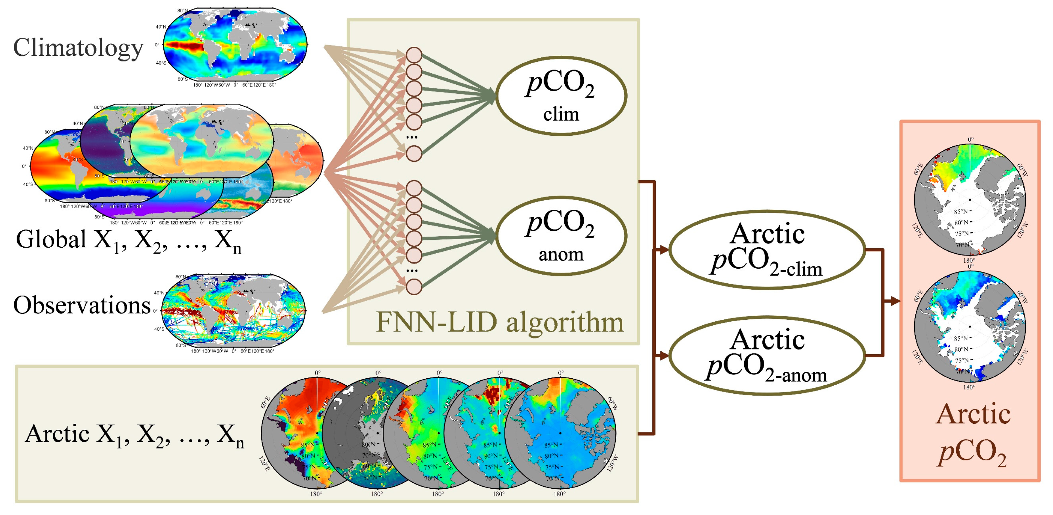
We used gridded sea surface temperature (SST), sea surface salinity (SSS), sea surface height (SSH), atmospheric CO2 mole fraction xCO2 (xCO2), Chl-a and mixed layer depth (MLD) datasets to train the FNN-LID model and reconstruct the pCO2 series (Table 2). The 0.25° monthly SST, SSS, SSH and MLD data were provided by the Copernicus Marine Environment Monitoring Service (CMEMS). The xCO2 data were acquired from the Copernicus Atmosphere Monitoring Service (CAMS) global atmospheric composition forecasts. In addition to the predictors listed in this table, the climatological pCO2 [5], latitude and longitude information were also used as predictors in the reconstruction. Furthermore, the sea ice concentration (percentage of the ocean area covered by sea ice concentration (SIC), sea level pressure, 10 m wind speed and total pressure were exploited to obtain the air–sea carbon flux. The SIC data were obtained from the NSIDC Climate Data Record at a spatial resolution of 25 km and a monthly temporal resolution [64]. The sea level pressure and 10 m wind speed data were derived from CALIOP (Section 2.2.2). We used the monthly total sea surface pressure data from the European Centre for Medium-Range Weather Forecasts (ECMWF) with a 1° spatial resolution.
In addition, the original data were interpolated into 1 × 1° cells. To create the diurnal pCO2 field and calculate the air–sea carbon flux in polar nighttime, we used all data available at diurnal resolution, including the wind speed, Chl-a, sea surface pressure, temperature and xCO2 data. These diurnal data have the same spatial resolution as the monthly average results. As for the satellite launched in 2006, there were no available CALIOP data for the 2001–2006 period. Thus, wind speeds extracted from the Cross-Calibrated Multi-Platform (CCMP) dataset and the Chl-a data from GlobColour were used to replace LiDAR data during 2001–2006.

2.3. FNN-LID Method

We combined novel FNN methods based on active and passive remote sensing data (FNN-LID) collected during the period from January 2001 to December 2020 at a monthly 1 × 1° resolution and reconstructed the diurnal pCO2 series since 2007 (Figure 4). We used Keras (available online: https://keras.io (accessed on 6 September 2022)), a high-level neural network Python library, for the training and evaluation of the FNN. The complexity of the problem and the number of data used for training jointly determines the number of neurons and FNN layers. We followed the empirical rule of a factor of 10 between the number of data and the connections to avoid overfitting [65].
We used a two-part method to establish nonlinear relationships between a suite of independent environmental predictors and pCO2. To improve the accuracy of the reconstruction, the two parts were both built separately for each month. First, we derived the relationships between the pCO2 climatology (pCO2-clim) series and environmental predictors (SST, SSS, SSH, Chl-a, MLD, longitude and latitude) based on the FFN method using the monthly climatology [5] data as the standard output. We developed an FFNN model with 5 layers. In the second part, the target was to reconstruct the pCO2 anomalies (pCO2-anom) series using another FFN method and the target sea surface pCO2-anom was computed as the differences between SOCATv2022 observations and monthly climatological pCO2 from the first step (=pCO2-SOCAT − pCO2-clim). During the second step, normalized pCO2-anom were reconstructed as a nonlinear function of normalized SST, SSS, SSH, Chl-a, MLD, xCO2, longitude and latitude. The SST, SSS, Chl-a are from the same datasets (see in Table 2); however, the roles of these datasets played in the two steps are different. In the first step, it is desired to reconstruct more desirable high spatial resolution pCO2-clim data (1° × 1°) by environmental parameters, as the Takahashi’s climate state data have the problem of low spatial resolution (4° × 5°). In the second step, the same datasets were used to capture the pCO2-anom by using the limited amount of measured data and the matching environmental data. Finally, we obtained pCO2 by adding anomalies to climate state.
In these two steps, the training datasets were expanded by combining data representing the previous month and the next month to cluster the seasonal cycle and increase the amount of data considered in this step. In addition, we divided the dataset into 3 parts for the FNN training (50%), evaluation (25%) and model validation (25%) processes. We trained the model separately for each month to improve the accuracy of the reconstruction results. K-fold cross-validation (K = 4) was used for the evaluation and validation of the FFNN. Five FNN tests were performed per month for each sampling fold, and each of these five runs was characterized by a different initial value chosen at random. From these five results, the best result was selected. Hence, we constructed 12 FNN models with 5 layers sharing a common architecture but trained on different data; the validation process is detailed in Section 3.1.
On this basis, we updated the input data to the diurnal CALIPSO sea surface Chl-a data collected from 2007 to 2020 and the diurnal xCO2 data from ECMWF. Thus, we reconstructed the diurnal and nocturnal pCO2 series from 2007 to 2021 at a monthly 1 × 1° resolution.

2.4. Global Air–Sea CO2 Flux Estimates

The global air–sea CO2 flux is often estimated by the bulk method:
f l u x = k w × s o l × p CO 2 w a t e r p CO 2 a i r × 1 S I C ,
where f l u x (mol m−2 yr−1) is the air–sea CO2 flux, k w is the gas transfer velocity, s o l is the solubility of CO2 in seawater (mol m−2 µatm−1), p CO 2 w a t e r (µatm) and p CO 2 a i r (µatm) are the partial pressure of ocean surface CO2 and atmospheric CO2 in the marine boundary layer and S I C is the ice fraction of ocean area covered by sea ice.
The gas exchange rate is often estimated using the following equation:
k w = 0.251 × U 10 × S c 660 0.5 ,
where U 10 is the wind speed 10 m above sea level and S c denotes the Schmidt number calculated from the SST and SSS based on the equation proposed by Wanninkhof (2014).
The CO2 solubility at the air–sea interface is calculated from the seawater temperature and salinity [27]. Although several equations have been proposed to parameterize k w as a function of U 10 , we used Equation (5), which has been widely used to estimate CO2 fluxes in Arctic studies (e.g., [66]). Throughout this study, the flux is defined as positive when CO2 is released from the ocean to the atmosphere and negative when CO2 is absorbed by the ocean from the atmosphere. The S I C is used because ice acts as an imperfect barrier to gas exchange [67,68,69]. However, whether the effect of sea ice on gas exchange is linear [68,70] or nonlinear [67,71] is still under debate; for simplicity, only a linear ice correction is used in this work. In addition, when SIC is larger than 99%, we use 99% to allow air–sea CO2 exchanges through fractures, leads and brine channels [72]. The sources of all data used here are provided in Section 2.
In this study, the air–sea carbon flux is commonly described through a bulk formula [27,73]. Therefore, we discuss the impacts of considering different carbon flux mechanisms in terms of day-night ratios as follows:
k k w = k w d a y k w n i g h t ,
k d p = p w a t e r _ d a y p a i r _ d a y p w a t e r _ n i g h t p a i r _ n i g h t = d p d a y d p n i g h t ,
f l u x d a y f l u x n i g h t = k w d a y k w n i g h t × d p d a y d p n i g h t = k s o l × k k w × k d p ,
where k k w and k d p represent the ratios of the air–sea exchange rate and the different components of the day and night durations, respectively. When this ratio is less than 1, it means that the parameter is higher during the night than during the day; when the ratio is greater than 1, it means that lower values appear at night.

2.5. Interpretation of Statistics

The root mean square error (RMSE), bias and Pearson correlation coefficient (R) were used in this work as standard statistical metrics to measure the model performance. The RMSE was calculated for the dataset as follows:
R M S E = 1 n i = 1 n O b s E s t i 2 ,
B i a s = 1 n i = 1 n E s t O b s i ,
where n is the sample index, O b s is the observation measurement and E s t is the model estimate.

3. Results

3.1. Validation of FNN-LID pCO2

The pCO2 values simulated by the fitted FFN-LID model were compared to the measurements extracted from SOCATv2022, with an overall mean R2 of 0.79 and an RMSE of 17.76 µatm (Figure 5A). The average difference between the observed and simulated pCO2 was almost null (overall bias = 0.1 µatm) globally and was −0.08 in the Arctic region (Figure 5B). The comparison of our Arctic FFN-LID results with the observations shows an average RMSE of 24.59 µatm and an overall mean R2 of 0.75; these values are comparable with the recent SOCAT-based global pCO2 fields in the Arctic Ocean (Table 3).
Compared to other datasets, we obtained a generally similar spatial distribution with spatially random residuals of −0.14 ± 15.98 µatm (Figure 5C), which is overestimated in the costal Beaufort Sea and the north of the Novaya Zemlya Island and slightly underestimated in the melted ice zone east of Greenland Island (Figure 5D). However, we found higher pCO2 (>400 µatm) values in the costal East Siberian and the Laptev Sea throughout the summer season; these values were higher than those provided by most global coverage models and were more consistent with other observation-based studies than the outputs of previous models.
As the East Siberian Sea is a blank area in the SOCAT datasets, we used the independent Global Ocean Data Analysis Project (GLOBDAP) dataset, an agglomerating chemical water analysis dataset with vertical information, to validate the high pCO2 we found in the FNN-LID outputs. Two consecutive GLOBDAP cruises passed through the region measured in August and September 2008, showing that the pCO2 of the continental shelf was high, even higher than that of the atmosphere (approximately 400 µatm) (Figure 6A,E). Compared to the IBP (Figure 6C,G) and CMEMS (Figure 6D,H) model outputs, we can clearly find that the pCO2 values retrieved by the FNN-LID model (Figure 6B,F) are closer to the summertime in situ spatial distribution, reconstructing the high-pCO2 waters in the continental shelf area.

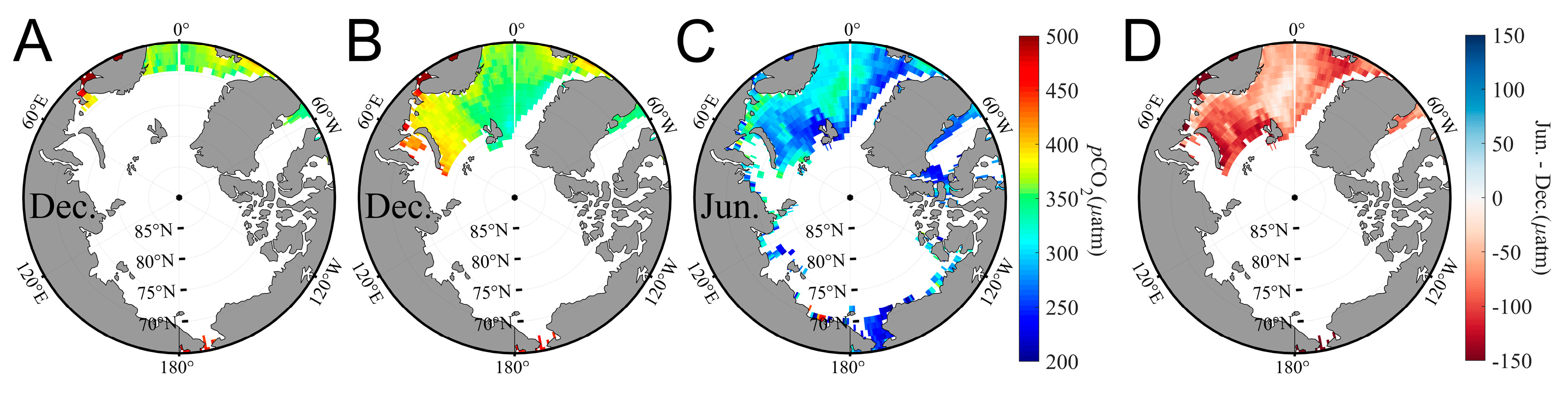
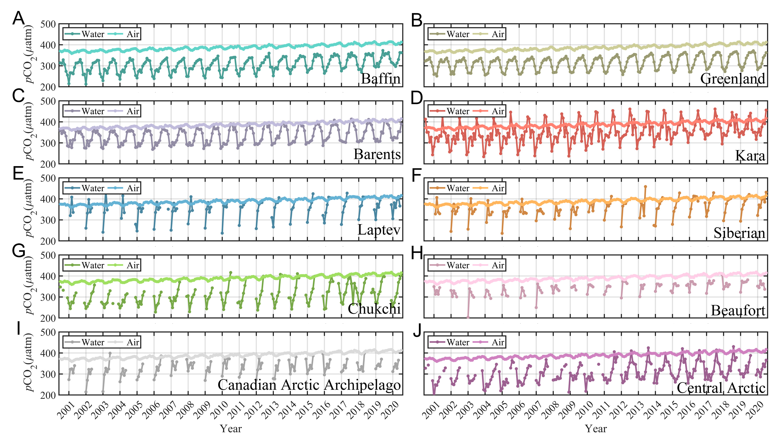
3.2. Sea Surface pCO2 during Polar Night and Seasonal Variations

Polar night is a period of continuous twilight or nighttime; polar night lasts approximately 11 weeks at the poles, and the North Pole experiences this period from November to January. During this time, the Arctic Ocean receives less radiation, and for more than one month the sun never rises at this pole during the whole 24 h of the day.
Although some models replace Arctic winter Chl-a values with the climatological average or interpolated Chl-a values, these statistical Chl-a values fill the wintertime pCO2 maps with potential errors. Due to the wintertime Chl-a values usually being lower than the climatological average values, such interpolation methods fail when edge data are missing. However, as CALIPSO measurements collected via active LiDAR sensing are not limited by solar radiation, the FNN-LID model can provide ‘fill-in’ values from the late autumn to early spring seasons to supplement the data hidden from ocean color sensors and thus construct the first complete record of polar pCO2. The December pCO2 data reconstructed using GlobColour Chl-a and LiDAR Chl-a data are shown in Figure 7A,B. Both these data sources can successfully reproduce the pCO2 distribution, but the LIDAR-based product has a clearly superior spatial coverage. Moreover, if the Arctic carbon sink were estimated directly using these relatively small-coverage data, the resulting Arctic carbon sink values would be underestimated.
In this framework, we assessed the complete seasonal cycle variations in the Arctic Oceans. Similar seasonal patterns and driving mechanisms are extracted by the Climate Model Intercomparison Project Version-5 (CMIP5) models under modern forcing conditions [74,75]. However, the modeled seasonal variations do not include the Arctic Ocean due to the sparsity of seasonal observations in this region. Thus, we exploited the FNN-LID-derived observation-based product to fill this observational gap. The results indicate that surface water pCO2 is higher in winter than in summer, suggesting that nonthermal effects dominate here, as in the subarctic region (Figure 7D). Taking the Greenland Sea and Barents Sea as examples, the seasonal variation (from June to December) in pCO2 in the Arctic Ocean seawater is found to be approximately 81.1 (±39.16) μatm; this seasonal variation is prevalent throughout the Arctic Ocean. In addition, seasonal amplitude maxima can be observed in the Bering Strait and along the shelf edge of the White Sea.

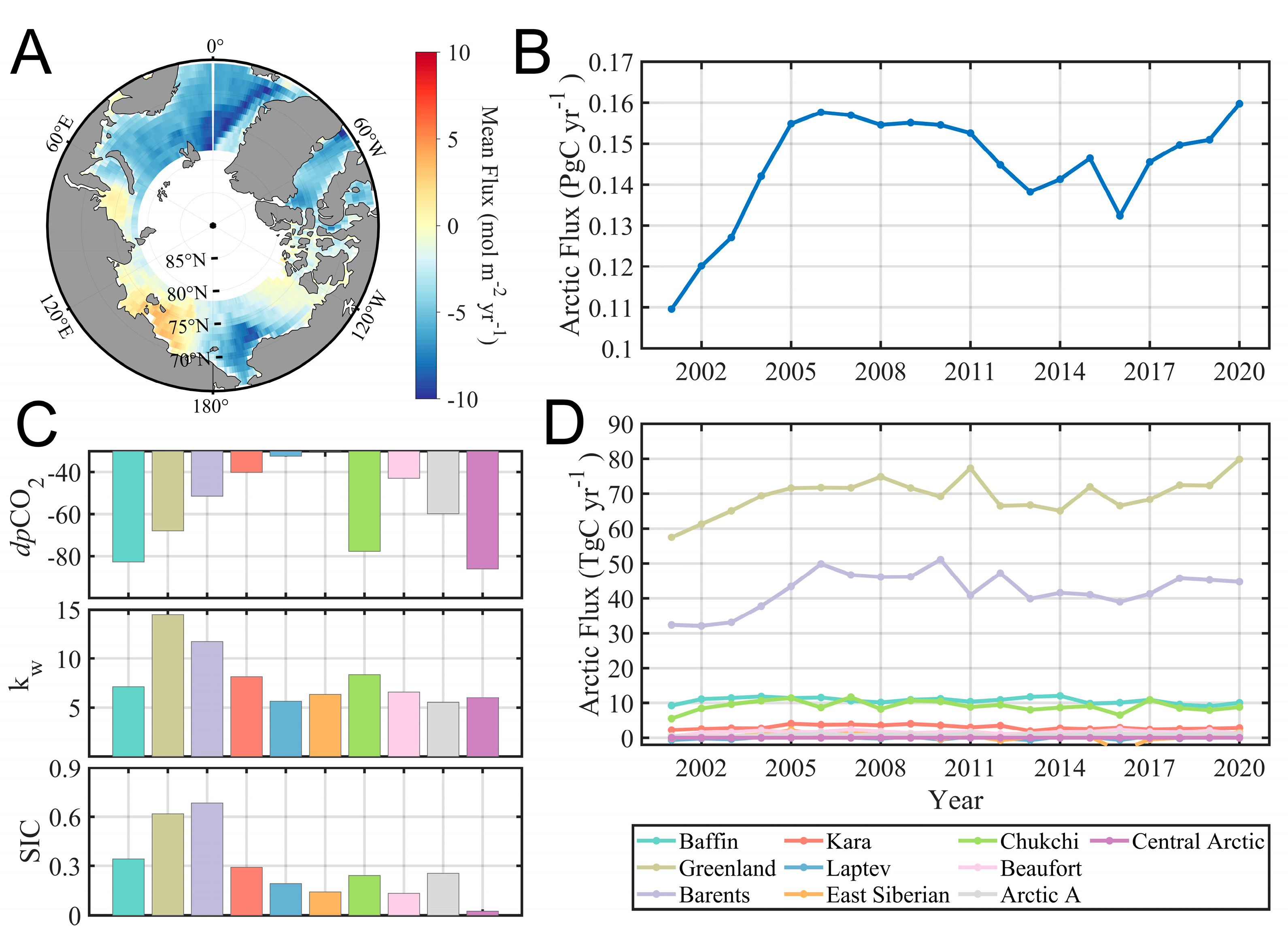
3.3. Distributions of Arctic Ocean pCO2 and Flux

Due to the coverage of sea ice in winter, year-round pCO2 data are not available for some sea ice-covered months, as sea ice can interfere with radiative transfer, causing the quality of remote sensing data to degrade. Thus, we used SIC to select the sea surface pCO2 rather than the subglacial pCO2; the resulting long-term monthly pCO2 series are shown in Figure 8. Based on the FNN-LID-derived pCO2, we found that the spatial pattern shows higher seasonal variations in the regions dominated by Pacific waters (e.g., the Chukchi Sea and the Greenland Sea), as illustrated in Figure 8B,G. In the Chukchi sector (Figure 8G), the sea surface pCO2 was higher than that in the western Beaufort Sea (Figure 8H); this finding is consistent with observations by Bates [22].
In addition, we found that there is little spatial variability in atmospheric pCO2 over the Arctic Oceans, with seasonal variations of ~4 μatm, reaching the highest value in summer (Figure 8). The seasonal variation in seawater pCO2 is nearly 20 times greater than that in atmospheric pCO2. The magnitude and direction of the release or uptake of CO2 across the sea surface are determined by the air–sea difference in pCO2. Over the last 20 years, atmospheric pCO2 has been experiencing a steady rise (2.0611 ± 0.03 μatm yr−1), with the annual average increase from 361.31 μatm to 402.12 μatm. Meanwhile, most Arctic Ocean surface pCO2 has been lower than the atmospheric pCO2 and has thus acted as a stable carbon sink, except in the Kara Sea, where seasonally high pCO2 occurs in winter (Figure 8D).
The 20-year annual CO2 sink per m2 was strong in the Greenland/Norwegian Seas (>4.45 mol m−2 yr−1), the Barents Sea (2.04 mol m−2 yr−1), Baffin Bay (2.75 mol m−2 yr−1) and the Chukchi Sea (2.38 mol m−2 yr−1) (Figure 9A). In contrast, it was weak (<1 mol m−2 yr−1) in the Kara Sea, the Beaufort Sea, the East Siberian and Canada Arctic Archipelago (Figure 9A). The annual mean CO2 flux distribution shows that most areas of the Arctic Ocean and its adjacent seas served as net CO2 sinks over the study period, showing a significant increase from 2001 to 2005 and remaining at 0.15 ± 0.01 TgC yr−1 over the next 15 years (Figure 9B). The SIC is the most fundamental element controlling the carbon flux magnitude, forcing a small carbon flux in the central Arctic Ocean. Both the Barents Sea and the Greenland Sea have very low sea ice cover and large sea gas pressure gaps, but the Greenland Sea has higher surface wind speeds that cause greater air–sea exchange rates; thus, the Greenland Sea has become the largest carbon flux partition zone in the Arctic (Figure 9C). Regarding the fluxes of individual sectors, the primary controlling factor for the monthly CO2 sink is the ice-covered area (equivalent to the ice%), and the secondary factor is the wind speed. In addition, the carbon flux is nearly null or even seasonally within uncertainty in the Laptev Sea (~approximately0.20 mol m−2 yr−1) and East Siberian Sea (approximately 0.36 mol m−2 yr−1). Previous measurement-based research has also indicated that the Laptev Sea and the East Siberian Arctic Shelf are sources of atmospheric CO2 [76,77,78]. These high pCO2 values could be explained by the increasing load of humid acids delivered to shelf waters, while more nutrients, as products of eroded organic carbon transformation and river transport, are delivered to the Arctic Ocean [79]. Meanwhile, due to the impacts of complex factors (such as river runoff, coastal erosion, and primary production/respiration), the year-to-year dynamics of pCO2 as well as the air–sea carbon flux vary substantially [80]. As the sampling frequency of the measured data receive restrictions to access pCO2 with high spatiotemporal coverage, the FNN-LID complements the seasonal lack of measurement and, once again, confirms this sector to be the seasonal source of atmospheric pCO2.

4. Discussion

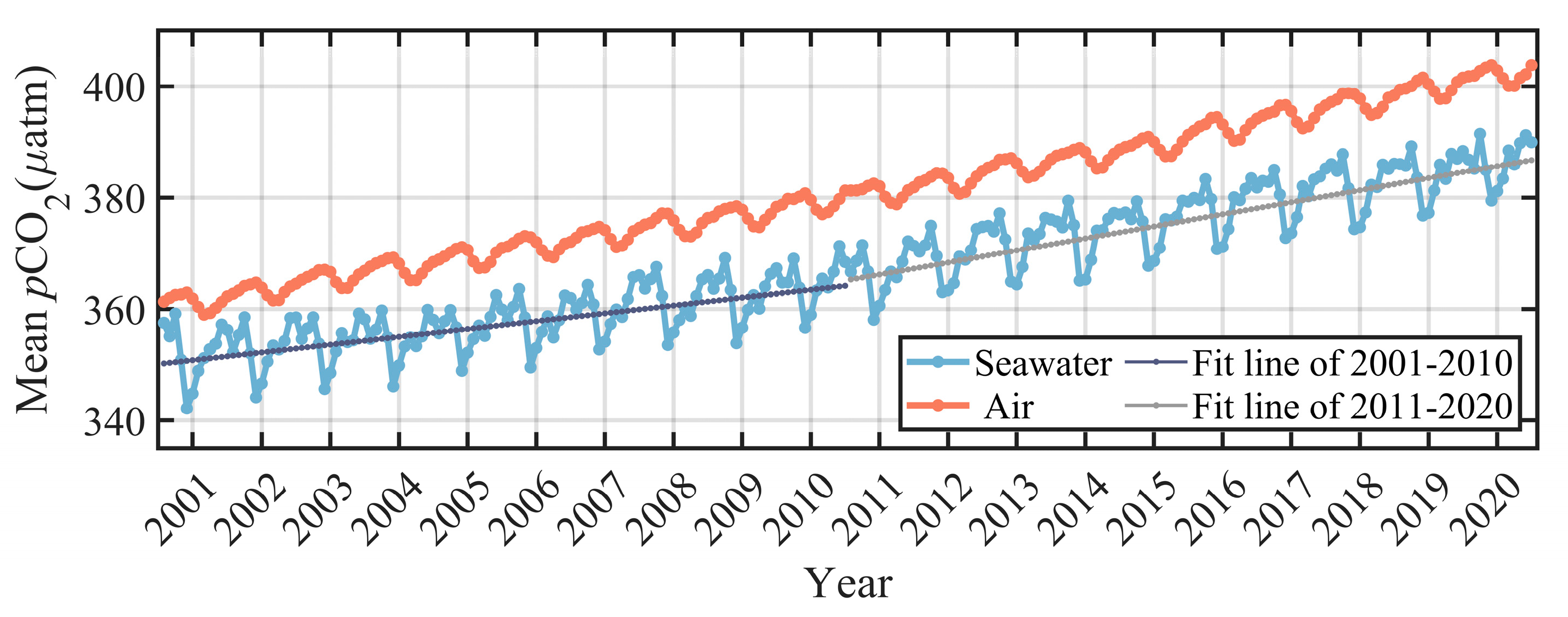
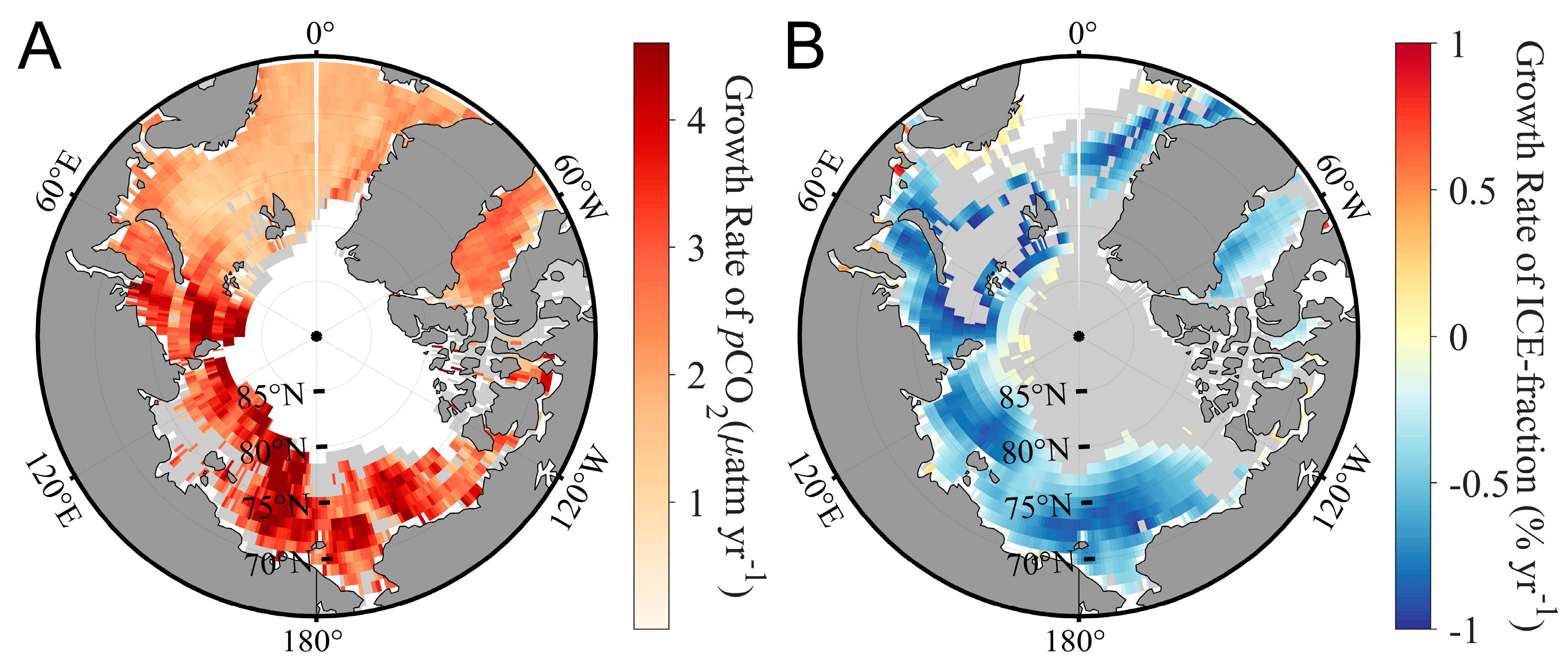
4.1. Long-Time-Series Variations in Arctic pCO2

We used long-time-series pCO2 values for individual months to calculate interannual trends, which allows us to reduce the impact of specific events that occur in particular months, such as abrupt changes due to surges in primary productivity in ice melt regions. The computed trends of the 20-year monthly values were approximately 1.41 ± 0.015 μatm yr−1 from 2001 to 2010 and 2.16 ± 0.019 μatm yr−1 for the next decade, indicating that the growth rate of Arctic seawater pCO2 is increasing (Figure 10). Accompanied by an almost unchanged growth rate of atmospheric pCO2 (2.17 ± 0.21 μatm yr−1), the trend in Arctic seawater has gradually become flatter than that in the atmosphere over the past 20 years, thus allowing the Arctic to be maintained as a stable carbon sink based on the perspective of sea–air interactions.
In addition, we also statistically estimated the trends of the spatial distributions of pCO2 and SIC declines (Figure 11A,B). We found that the growth rates of sea surface pCO2 were remarkable in regions with significant sea ice retreat, such as the East Siberian Sea and the Kara Sea. Based on years of observation measurements, Qi et al., 2022 summarized that when sea ice is lost, the well-buffered seawater with relatively high alkalinity and low pCO2 near the sea ice is diluted by the meltwater with relatively low alkalinity, high pCO2 and a low buffer capacity [81]. Thus, atmospheric CO2 invasion would result in greater overall declines in the pH and buffer capacity metrics in seawater diluted by meltwater compared to the original water. This ice-melt-driven mechanism can explain the amplified rapid increase in pCO2 observed in the Arctic Ocean over the past two decades.

4.2. Diurnal Carbon Fluxes and Mechanism Analysis in the Arctic

It is well known that near-equal day and night durations occur only in spring and autumn in extremely high latitudes. The March and September equinoxes mark the two days of each year when day and night are of equal length, with 12 h of daylight and 12 h of darkness at all points on the Earth’s surface. Therefore, for simplicity, we discuss only March and June data when studying the intraday diurnal variations in carbon fluxes in the Arctic Ocean.
Based on the data retrieved from CALIPSO, the distribution of chlorophyll in the Arctic Ocean quite clearly reveals diurnal variations, and the spatial distribution of surface Chl-a is marked by high values on the continental shelf ranging from 0.7 to >3.0 μg L−1, reflecting higher nutrient concentrations and rates of primary production, while the Chl-a values generally range from 0.05 to 0.3 μg L−1 in the deep central Arctic Ocean (Figure 12A–D) [82]. The day/night ratio is higher than 1 in these regions, implying that the water column at 50 m above the sea surface has higher Chl-a during the day (Figure 12E,F). This area is influenced by several large rivers, and the low latitude zone located in the Arctic Ocean experiences relatively high insolation. Both in spring (March) and autumn (September), Chl-a is higher during the day than at night. It is of note that the Carbon C:Chl-a model of Behrenfeld et al., 2016, which represents an upper end model of the photo acclimation response, and the regression analyses of phytoplankton division from the Standard Model and values from any of the Alternative Models give coefficients of determination of r2 = 0.99 for both the North and South Polar Zones, indicating that the model variations slightly impact the amplitude of phytoplankton division values but have negligible impact on the annual cycles [83]. By contrast, the model of Westberry et al. (2008) assigns a very conservative fraction of C:Chl-a variability to photo acclimation and thus represents a lower end response model [84]. In the future, we will seek to study and establish a direct relationship between the LiDAR signal and chlorophyll using a machine learning method to avoid the spatio-temporal variability of C: Chl-a.
Phytoplankton and the diel vertical migration (DVM) of animals together determine diurnal b b p changes; in the absence of any DVM, the biomass-normalized b b p is expected to be greater in diurnal than nocturnal due to the increase in phytoplankton cell size and organic carbon content during the day and cell division and metabolism at night [85,86,87,88]. These diurnal differences create a baseline diurnal cycle in the biomass-normalized b b p with a maximum in the afternoon and a minimum at night [85]. However, the presence of DVM animals increases b b p at night and therefore causes diurnal b b p difference to become less negative than the phytoplankton-only signal. Thus, our diurnal difference from the CALIPSO signal may be underestimated, which means the actual Chl-a diurnal difference is larger than the current results.
In spring and autumn, in general, the daytime dpCO2 is slightly smaller than the nighttime dpCO2 (92.8% on average for the whole Arctic Ocean), while relatively large diurnal variations occur in a small range of coastal water masses, such as the Kara Sea estuary (the green region in Figure 13D). Compared to spring, autumn ice retreat is more widespread, and we can observe a significant amount of daytime Chl-a along the shores of the Laptev and East Siberian Seas. This phenomenon also causes higher autumn pCO2 regionally, with values even higher than those in the atmosphere, thus resulting in a seasonal small-regional carbon source (the purple region in Figure 13F). In conclusion, except for some small nearshore estuarine regions, the Arctic Ocean is a stable carbon sink regardless of day and night.
In contrast, wind speeds show an interesting parahemispheric distribution bounded by Novaya Zemlya and Greenland, with higher daytime than nighttime winds in Baffin Bay, the Greenland Sea, the Barents Sea and the Kara Sea (with a mean diurnal ratio of approximately 101.1%) and higher nighttime winds in the Siberian Sea, the Chukchi Sea of the Lavetev Sea and the Canadian Arctic Archipelago (with a mean diurnal ratio of approximately 93.9%); this distribution pattern is not altered by seasonal changes (Figure 13B,E). Consequently, the spatial combination of the sea surface partial pressure and wind speed affects the diurnal carbon sink in the Arctic. On the Atlantic side, the partial pressure difference and the wind speed exert opposite effects, whereby the magnitude of the wind speed eventually becomes the main controlling mechanism, thus resulting in a larger absorption rate during the day than at night (Figure 13C,F). On the Pacific side, the partial pressure difference and wind speed are shown to be higher at night, and together, these conditions cause the diurnal absorption rate to be smaller in the daytime than at night (Figure 13F).

5. Conclusions

In this study, we foremost constructed an FFN-LID model to derive Arctic pCO2 and formed a long-time-series dataset containing variations in air–sea CO2 fluxes from 2001 to 2020 as well as diurnal products from 2007 to 2020.
Not only are the normal passive remote sensing products used in this work, but CALIPSO-recorded Chl-a and wind speed data are also added as inputs to build the FNN-LID model. This is the first time LiDAR has been employed in research on the Arctic air–sea carbon cycle. The CloudSat and Cloud-Aerosol Lidar and Infrared Pathfinder Satellite Observation (CALIPSO) platform can provide data not only at a large coverage, including the polar regions, but can also provide a clearer understanding of global diurnal pCO2 variations. Although some models replace Arctic winter Chl-a data with the climatological average or interpolated Chl-a values, these statistical Chl-a values result in the gap-filled wintertime pCO2 map having potential errors. The CALIPSO measurements obtained through active LiDAR sensing are not limited by solar radiation and can thus provide ‘fill-in’ data for the late autumn to early spring seasons to compensate for data missing from ocean color sensors; in this way, we were able to construct the first complete record of polar pCO2.
By analyzing the FNN-LID results, we found that the Arctic pCO2 exhibited different spatial characteristics during the day and night. The FFN-LID model fitted the measurements with an overall mean R2 of 0.75 and an average RMSE of 24.59 µatm in the Arctic and could better reconstruct values in two high-pCO2 sectors (the Laptev Sea and the East Siberian Sea) compared to other models. The FNN-LID observation-based product fills the observational gaps in wintertime, indicating that the surface water pCO2 is higher in winter than in summer (e.g., approximately 81.1 ± 39.16 μatm in the Greenland Sea and Barents Sea). The Arctic Ocean net CO2 sinks showed a significant increase from 2001 to 2005 and remained at 0.15 ± 0.01 TgC yr−1 over the next 15 years with seasonal sources on some continental shelves. The primary factor controlling the CO2 sink was the percentage of ice-covered areas. In addition, we found that the computed growth rate of Arctic seawater pCO2 was increasing over the study period and that the corresponding growth rates were remarkable in sectors with significant sea ice retreat.
The water column at 50 m above the sea surface has higher Chl-a values during the day than at night in spring and autumn. In addition, the spatial combination of the sea surface partial pressure and wind speed affects the diurnal carbon sink in the Arctic: the partial pressure difference and the wind speed exert opposite effects, whereby the magnitude of the wind speed eventually becomes the main controlling mechanism, thus resulting in a larger absorption rate during the day on the Atlantic side. However, on the Pacific side, the partial pressure difference and wind speed are shown to be higher at night, and together, these factors cause the diurnal absorption rate to be smaller in the daytime than at night.
The model constructed herein extends the study of remote sensing data with regard to polar research and diurnal variations. With the accumulation of remote sensing data, we plan to further extend our study of carbonate systems in other sea ice regions and to try to use higher-resolution spatial data to analyze carbonate systems in nearshore and coastal ecosystems. Meanwhile, both C: Chl-a variability and DVM affect the results of the model; our next step will be to analyze in more detail and try to clarify the contribution ratio of diurnal variation and DVM in the change of the b b p signal for a better understanding and awareness of pCO2.

Author Contributions

Conceptualization, S.Z. and P.C.; methodology, S.Z., Z.Z. and P.C.; investigation, D.P.; writing—original draft preparation, S.Z.; writing—review and editing, P.C.; funding acquisition, D.P. All authors have read and agreed to the published version of the manuscript.

Funding

This research was funded by the National Key Research and Development Program of China (2022YFB3901703), the Key Special Project for the Introduced Talents Team of the Southern Marine Science and Engineering Guangdong Laboratory (GML2021GD0809), the National Natural Science Foundation (42276180; 41901305; 61991453) and the Key Research and Development Program of Zhejiang Province (2020C03100).

Data Availability Statement

Not applicable here.

Acknowledgments

The authors are grateful to the NASA Langley Research Center for providing CALIOP data through the Atmospheric Sciences Data Center (https://asdc.larc.nasa.gov/data/CALIPSO/ (accessed on 9 August 2022)). We thank the NASA Marine Biology Processing Group and Globe Color for also providing MODIS products (https://oceandata.sci.gsfc.nasa.gov/ (accessed on 10 September 2022)). We thank the anonymous reviewers for their suggestions, which significantly improved the presentation of the paper.

Conflicts of Interest

The authors declare no conflict of interest.

References

  1. Gruber, N.; Clement, D.; Carter, B.R.; Feely, R.A.; Van Heuven, S.; Hoppema, M.; Ishii, M.; Key, R.M.; Kozyr, A.; Lauvset, S.K. The oceanic sink for anthropogenic CO2 from 1994 to 2007. Science 2019, 363, 1193–1199. [Google Scholar] [CrossRef] [PubMed] [Green Version]
  2. McNeil, B.I.; Sasse, T.P. Future ocean hypercapnia driven by anthropogenic amplification of the natural CO2 cycle. Nature 2016, 529, 383–386. [Google Scholar] [CrossRef] [PubMed]
  3. Takahashi, T.; Olafsson, J.; Goddard, J.G.; Chipman, D.W.; Sutherland, S. Seasonal variation of CO2 and nutrients in the high-latitude surface oceans: A comparative study. Glob. Biogeochem. Cycles 1993, 7, 843–878. [Google Scholar] [CrossRef]
  4. Sarmiento, J.L. Ocean biogeochemical dynamics. In Ocean Biogeochemical Dynamics; Princeton University Press: Princeton, NJ, USA, 2013. [Google Scholar]
  5. Takahashi, T.; Sutherland, S.C.; Wanninkhof, R.; Sweeney, C.; Feely, R.A.; Chipman, D.W.; Hales, B.; Friederich, G.; Chavez, F.; Sabine, C. Climatological mean and decadal change in surface ocean pCO2, and net sea–air CO2 flux over the global oceans. Deep Sea Res. Part II Top. Stud. Oceanogr. 2009, 56, 554–577. [Google Scholar] [CrossRef]
  6. Takahashi, T.; Sutherland, S.C.; Chipman, D.W.; Goddard, J.G.; Ho, C.; Newberger, T.; Sweeney, C.; Munro, D. Climatological distributions of pH, pCO2, total CO2, alkalinity, and CaCO3 saturation in the global surface ocean, and temporal changes at selected locations. Mar. Chem. 2014, 164, 95–125. [Google Scholar] [CrossRef] [Green Version]
  7. Bates, N.R.; Astor, Y.M.; Church, M.J.; Currie, K.; Dore, J.E.; González-Dávila, M.; Lorenzoni, L.; Muller-Karger, F.; Olafsson, J.; Santana-Casiano, J.M. A time-series view of changing surface ocean chemistry due to ocean uptake of anthropogenic CO2 and ocean acidification. Oceanography 2014, 27, 126–141. [Google Scholar] [CrossRef] [Green Version]
  8. Rödenbeck, C.; Bakker, D.C.; Gruber, N.; Iida, Y.; Jacobson, A.R.; Jones, S.; Landschützer, P.; Metzl, N.; Nakaoka, S.-I.; Olsen, A. Data-based estimates of the ocean carbon sink variability–first results of the Surface Ocean pCO 2 Mapping intercomparison (SOCOM). Biogeosciences 2015, 12, 7251–7278. [Google Scholar] [CrossRef] [Green Version]
  9. Le Quéré, C.; Andrew, R.M.; Friedlingstein, P.; Sitch, S.; Pongratz, J.; Manning, A.C.; Korsbakken, J.I.; Peters, G.P.; Canadell, J.G.; Jackson, R.B. Global carbon budget 2017. Earth Syst. Sci. Data 2018, 10, 405–448. [Google Scholar] [CrossRef] [Green Version]
  10. Sabine, C.L.; Feely, R.A.; Gruber, N.; Key, R.M.; Lee, K.; Bullister, J.L.; Wanninkhof, R.; Wong, C.; Wallace, D.W.; Tilbrook, B. The oceanic sink for anthropogenic CO2. Science 2004, 305, 367–371. [Google Scholar] [CrossRef] [Green Version]
  11. IPCC. Impacts, Adaptation, and Vulnerability. Part A: Global and Sectoral Aspects. Contribution of Working Group II to the Fifth Assessment Report of the Intergovernmental Panel on Climate Change; Cambridge University Press: Cambridge, UK; New York, NY, USA, 2014; pp. 1–32. [Google Scholar]
  12. Onarheim, I.H.; Eldevik, T.; Smedsrud, L.H.; Stroeve, J.C. Seasonal and regional manifestation of Arctic sea ice loss. J. Clim. 2018, 31, 4917–4932. [Google Scholar] [CrossRef]
  13. Stroeve, J.; Notz, D. Changing state of Arctic sea ice across all seasons. Environ. Res. Lett. 2018, 13, 103001. [Google Scholar] [CrossRef]
  14. Timmermans, M.L.; Proshutinsky, A.; Golubeva, E.; Jackson, J.; Krishfield, R.; McCall, M.; Platov, G.; Toole, J.; Williams, W.; Kikuchi, T. Mechanisms of Pacific summer water variability in the Arctic’s Central Canada Basin. J. Geophys. Res. Ocean. 2014, 119, 7523–7548. [Google Scholar] [CrossRef] [Green Version]
  15. Corlett, W.B.; Pickart, R.S. The Chukchi slope current. Prog. Oceanogr. 2017, 153, 50–65. [Google Scholar] [CrossRef] [Green Version]
  16. Stabeno, P.; Kachel, N.; Ladd, C.; Woodgate, R. Flow patterns in the eastern Chukchi Sea: 2010–2015. J. Geophys. Res. Ocean. 2018, 123, 1177–1195. [Google Scholar] [CrossRef]
  17. Giles, K.A.; Laxon, S.W.; Ridout, A.L.; Wingham, D.J.; Bacon, S. Western Arctic Ocean freshwater storage increased by wind-driven spin-up of the Beaufort Gyre. Nat. Geosci. 2012, 5, 194–197. [Google Scholar] [CrossRef]
  18. Yamamoto-Kawai, M.; McLaughlin, F.; Carmack, E.; Nishino, S.; Shimada, K.; Kurita, N. Surface freshening of the Canada Basin, 2003–2007: River runoff versus sea ice meltwater. J. Geophys. Res. Ocean. 2009, 114, C00A05. [Google Scholar] [CrossRef]
  19. Arrigo, K.R.; van Dijken, G.L. Continued increases in Arctic Ocean primary production. Prog. Oceanogr. 2015, 136, 60–70. [Google Scholar] [CrossRef]
  20. Yamamoto-Kawai, M.; McLaughlin, F.A.; Carmack, E.C.; Nishino, S.; Shimada, K. Aragonite undersaturation in the Arctic Ocean: Effects of ocean acidification and sea ice melt. Science 2009, 326, 1098–1100. [Google Scholar] [CrossRef] [Green Version]
  21. Arctic Monitoring and Assessment Programme (AMAP). Arctic Ocean Acidification Assessment: 2018 Summary for Policy-Makers; AMAP: Oslo, Norway, 2019. [Google Scholar]
  22. Bates, N.R.; Moran, S.B.; Hansell, D.A.; Mathis, J.T. An increasing CO2 sink in the Arctic Ocean due to sea-ice loss. Geophys. Res. Lett. 2006, 33, L23609. [Google Scholar] [CrossRef] [Green Version]
  23. Cai, W.-J.; Chen, L.; Chen, B.; Gao, Z.; Lee, S.H.; Chen, J.; Pierrot, D.; Sullivan, K.; Wang, Y.; Hu, X. Decrease in the CO2 uptake capacity in an ice-free Arctic Ocean basin. Science 2010, 329, 556–559. [Google Scholar] [CrossRef]
  24. Else, B.G.; Galley, R.; Lansard, B.; Barber, D.; Brown, K.; Miller, L.; Mucci, A.; Papakyriakou, T.; Tremblay, J.É.; Rysgaard, S. Further observations of a decreasing atmospheric CO2 uptake capacity in the Canada Basin (Arctic Ocean) due to sea ice loss. Geophys. Res. Lett. 2013, 40, 1132–1137. [Google Scholar] [CrossRef] [Green Version]
  25. Ouyang, Z.; Qi, D.; Chen, L.; Takahashi, T.; Zhong, W.; DeGrandpre, M.D.; Chen, B.; Gao, Z.; Nishino, S.; Murata, A. Sea-ice loss amplifies summertime decadal CO2 increase in the western Arctic Ocean. Nat. Clim. Chang. 2020, 10, 678–684. [Google Scholar] [CrossRef]
  26. Euskirchen, E.S.; Bruhwiler, L.M.; Commane, R.; Parmentier, F.-J.W.; Schädel, C.; Schuur, E.A.; Watts, J. Current knowledge and uncertainties associated with the Arctic greenhouse gas budget. In Balancing Greenhouse Gas Budgets; Elsevier: Amsterdam, The Netherlands, 2022; pp. 159–201. [Google Scholar]
  27. Wanninkhof, R. Relationship between wind speed and gas exchange over the ocean revisited. Limnol. Oceanogr. Methods 2014, 12, 351–362. [Google Scholar] [CrossRef]
  28. Cole, J.J.; Caraco, N.F. Atmospheric exchange of carbon dioxide in a low-wind oligotrophic lake measured by the addition of SF6. Limnol. Oceanogr. 1998, 43, 647–656. [Google Scholar] [CrossRef] [Green Version]
  29. Blomquist, B.W.; Huebert, B.J.; Fairall, C.W.; Bariteau, L.; Edson, J.B.; Hare, J.E.; McGillis, W.R. Advances in Air–Sea CO2 Flux Measurement by Eddy Correlation. Bound. -Layer Meteorol. 2014, 152, 245–276. [Google Scholar] [CrossRef] [Green Version]
  30. Thornton, B.F.; Prytherch, J.; Andersson, K.; Brooks, I.M.; Salisbury, D.; Tjernström, M.; Crill, P.M. Shipborne eddy covariance observations of methane fluxes constrain Arctic sea emissions. Sci. Adv. 2020, 6, eaay7934. [Google Scholar] [CrossRef] [PubMed] [Green Version]
  31. Metcalfe, D.B.; Hermans, T.D.; Ahlstrand, J.; Becker, M.; Berggren, M.; Björk, R.G.; Björkman, M.P.; Blok, D.; Chaudhary, N.; Chisholm, C. Patchy field sampling biases understanding of climate change impacts across the Arctic. Nat. Ecol. Evol. 2018, 2, 1443–1448. [Google Scholar] [CrossRef]
  32. Arrigo, K.R.; Pabi, S.; van Dijken, G.L.; Maslowski, W. Air-sea flux of CO2 in the Arctic Ocean, 1998–2003. J. Geophys. Res. Biogeosciences 2010, 115, G04024. [Google Scholar] [CrossRef]
  33. Lefèvre, N.; Watson, A.J.; Watson, A.R. A comparison of multiple regression and neural network techniques for mapping in situ pCO2 data. Tellus B: Chem. Phys. Meteorol. 2005, 57, 375–384. [Google Scholar] [CrossRef] [Green Version]
  34. Friedrich, T.; Oschlies, A. Neural network-based estimates of North Atlantic surface pCO2 from satellite data: A methodological study. J. Geophys. Res. Ocean. 2009, 114, C03020. [Google Scholar] [CrossRef]
  35. Landschützer, P.; Gruber, N.; Bakker, D.C.; Schuster, U.; Nakaoka, S.-i.; Payne, M.R.; Sasse, T.P.; Zeng, J. A neural network-based estimate of the seasonal to inter-annual variability of the Atlantic Ocean carbon sink. Biogeosciences 2013, 10, 7793–7815. [Google Scholar] [CrossRef] [Green Version]
  36. Nakaoka, S.-i.; Telszewski, M.; Nojiri, Y.; Yasunaka, S.; Miyazaki, C.; Mukai, H.; Usui, N. Estimating temporal and spatial variation of ocean surface pCO 2 in the North Pacific using a self-organizing map neural network technique. Biogeosciences 2013, 10, 6093–6106. [Google Scholar] [CrossRef] [Green Version]
  37. Laruelle, G.G.; Landschützer, P.; Gruber, N.; Tison, J.-L.; Delille, B.; Regnier, P. Global high-resolution monthly pCO 2 climatology for the coastal ocean derived from neural network interpolation. Biogeosciences 2017, 14, 4545–4561. [Google Scholar] [CrossRef] [Green Version]
  38. Denvil-Sommer, A.; Gehlen, M.; Vrac, M.; Mejia, C. ffnn-lsce: A two-step neural network model for the reconstruction of surface ocean pco 2 over the global ocean. Geosci. Model Dev. 2019, 12, 2091–2105. [Google Scholar] [CrossRef] [Green Version]
  39. Chau, T.T.T.; Gehlen, M.; Chevallier, F. A seamless ensemble-based reconstruction of surface ocean pCO 2 and air–sea CO 2 fluxes over the global coastal and open oceans. Biogeosciences 2022, 19, 1087–1109. [Google Scholar] [CrossRef]
  40. Yasunaka, S.; Murata, A.; Watanabe, E.; Chierici, M.; Fransson, A.; van Heuven, S.; Hoppema, M.; Ishii, M.; Johannessen, T.; Kosugi, N. Mapping of the air–sea CO2 flux in the Arctic Ocean and its adjacent seas: Basin-wide distribution and seasonal to interannual variability. Polar Sci. 2016, 10, 323–334. [Google Scholar] [CrossRef]
  41. Yasunaka, S.; Siswanto, E.; Olsen, A.; Hoppema, M.; Watanabe, E.; Fransson, A.; Chierici, M.; Murata, A.; Lauvset, S.K.; Wanninkhof, R. Arctic Ocean CO 2 uptake: An improved multiyear estimate of the air–sea CO 2 flux incorporating chlorophyll a concentrations. Biogeosciences 2018, 15, 1643–1661. [Google Scholar] [CrossRef] [Green Version]
  42. Behrenfeld, M.J.; Hu, Y.; O’Malley, R.T.; Boss, E.S.; Hostetler, C.A.; Siegel, D.A.; Sarmiento, J.L.; Schulien, J.; Hair, J.W.; Lu, X. Annual boom–bust cycles of polar phytoplankton biomass revealed by space-based lidar. Nat. Geosci. 2017, 10, 118–122. [Google Scholar] [CrossRef]
  43. Lu, X.; Hu, Y.; Trepte, C.; Zeng, S.; Churnside, J.H. Ocean subsurface studies with the CALIPSO spaceborne lidar. J. Geophys. Res. Ocean. 2014, 119, 4305–4317. [Google Scholar] [CrossRef]
  44. Hu, Y.; Stamnes, K.; Vaughan, M.; Pelon, J.; Weimer, C.; Wu, D.; Cisewski, M.; Sun, W.; Yang, P.; Lin, B. Sea surface wind speed estimation from space-based lidar measurements. Atmos. Chem. Phys. 2008, 8, 3593–3601. [Google Scholar] [CrossRef]
  45. Hu, Y.; Winker, D.; Vaughan, M.; Lin, B.; Omar, A.; Trepte, C.; Flittner, D.; Yang, P.; Nasiri, S.L.; Baum, B. CALIPSO/CALIOP cloud phase discrimination algorithm. J. Atmos. Ocean. Technol. 2009, 26, 2293–2309. [Google Scholar] [CrossRef] [Green Version]
  46. Lu, X.; Hu, Y.; Yang, Y.; Bontempi, P.; Omar, A.; Baize, R. Antarctic spring ice-edge blooms observed from space by ICESat-2. Remote Sens. Environ. 2020, 245, 111827. [Google Scholar] [CrossRef]
  47. Dionisi, D.; Brando, V.E.; Volpe, G.; Colella, S.; Santoleri, R. Seasonal distributions of ocean particulate optical properties from spaceborne lidar measurements in Mediterranean and Black Sea. Remote Sens. Environ. 2020, 247, 111889. [Google Scholar] [CrossRef]
  48. Jamet, C.; Mj, B.; Ab, D.; Ov, K.; Ibrahim, A.; Ahmad, Z.; Angelini, F.; Babin, M.; J Behrenfeld, M.; Boss, E.; et al. Going Beyond Standard Ocean Color Observations: Lidar and Polarimetry. Front. Mar. Sci. 2019, 6, 251. [Google Scholar] [CrossRef]
  49. Hostetler, C.A.; Behrenfeld, M.J.; Hu, Y.; Hair, J.W.; Schulien, J.A. Spaceborne Lidar in the Study of Marine Systems. Annu. Rev. Mar. Sci. 2018, 10, 121–147. [Google Scholar] [CrossRef] [Green Version]
  50. Pfeil, B.; Olsen, A.; Bakker, D.C.; Hankin, S.; Koyuk, H.; Kozyr, A.; Malczyk, J.; Manke, A.; Metzl, N.; Sabine, C.L. A uniform, quality controlled Surface Ocean CO 2 Atlas (SOCAT). Earth Syst. Sci. Data 2013, 5, 125–143. [Google Scholar] [CrossRef] [Green Version]
  51. Sabine, C.L.; Hankin, S.; Koyuk, H.; Bakker, D.C.; Pfeil, B.; Olsen, A.; Metzl, N.; Kozyr, A.; Fassbender, A.; Manke, A. Surface Ocean CO 2 Atlas (SOCAT) gridded data products. Earth Syst. Sci. Data 2013, 5, 145–153. [Google Scholar] [CrossRef] [Green Version]
  52. Bakker, D.C.; Pfeil, B.; Landa, C.S.; Metzl, N.; O’brien, K.M.; Olsen, A.; Smith, K.; Cosca, C.; Harasawa, S.; Jones, S.D. A multi-decade record of high-quality fCO 2 data in version 3 of the Surface Ocean CO 2 Atlas (SOCAT). Earth Syst. Sci. Data 2016, 8, 383–413. [Google Scholar] [CrossRef] [Green Version]
  53. Körtzinger, A. Chap. Determination of carbon dioxide partial pressure (pCO2). In Methods of Seawater Analysis; WILEY: Hoboken, NJ, USA, 1999; pp. 149–158. [Google Scholar]
  54. Weiss, H.R. Control of myocardial oxygenation—Effect of atrial pacing. Microvasc. Res. 1974, 8, 362–376. [Google Scholar] [CrossRef] [PubMed]
  55. Olsen, A.; Key, R.M.; Van Heuven, S.; Lauvset, S.K.; Velo, A.; Lin, X.; Schirnick, C.; Kozyr, A.; Tanhua, T.; Hoppema, M. The Global Ocean Data Analysis Project version 2 (GLODAPv2)–an internally consistent data product for the world ocean. Earth Syst. Sci. Data 2016, 8, 297–323. [Google Scholar] [CrossRef]
  56. Olsen, A.; Lange, N.; Key, R.M.; Tanhua, T.; Bittig, H.C.; Kozyr, A.; Álvarez, M.; Azetsu-Scott, K.; Becker, S.; Brown, P.J. An updated version of the global interior ocean biogeochemical data product, GLODAPv2. 2020. Earth Syst. Sci. Data 2020, 12, 3653–3678. [Google Scholar] [CrossRef]
  57. Kim, M.-H.; Omar, A.H.; Tackett, J.L.; Vaughan, M.A.; Winker, D.M.; Trepte, C.R.; Hu, Y.; Liu, Z.; Poole, L.R.; Pitts, M.C. The CALIPSO version 4 automated aerosol classification and lidar ratio selection algorithm. Atmos. Meas. Tech. 2018, 11, 6107–6135. [Google Scholar] [CrossRef] [Green Version]
  58. Behrenfeld, M.; Hu, Y.; Bisson, K.; Lu, X.; Westberry, T. Retrieval of ocean optical and plankton properties with the satellite Cloud-Aerosol Lidar with Orthogonal Polarization (CALIOP) sensor: Background, data processing, and validation status. Remote Sens. Environ. 2022, 281, 113235. [Google Scholar] [CrossRef]
  59. Lu, X.; Hu, Y.; Vaughan, M.; Rodier, S.; Omar, A. New attenuated backscatter profile by removing the CALIOP receiver’s transient response. J. Quant. Spectrosc. Radiat. Transf. 2020, 255, 107244. [Google Scholar] [CrossRef]
  60. Behrenfeld, M.J.; Hu, Y.; Hostetler, C.A.; Dall”Olmo, G.; Rodier, S.D.; Hair, J.W.; Trepte, C.R. Space-based lidar measurements of global ocean carbon stocks. Geophys. Res. Lett. 2013, 40, 4355–4360. [Google Scholar] [CrossRef]
  61. Bisson, K.M.; Boss, E.; Werdell, P.J.; Ibrahim, A.; Behrenfeld, M.J. Particulate Backscattering in the Global Ocean: A Comparison of Independent Assessments. Geophys. Res. Lett. 2021, 48, e2020GL090909. [Google Scholar] [CrossRef]
  62. Li, J.; Hu, Y.; Huang, J.; Stamnes, K.; Yi, Y.; Stamnes, S. A new method for retrieval of the extinction coefficient of water clouds by using the tail of the CALIOP signal. Atmos. Chem. Phys. 2011, 11, 2903–2916. [Google Scholar] [CrossRef] [Green Version]
  63. Murphy, A.; Hu, Y. Retrieving Aerosol Optical Depth and High Spatial Resolution Ocean Surface Wind Speed From CALIPSO: A Neural Network Approach. Front. Remote Sens. 2021, 1, 614029. [Google Scholar] [CrossRef]
  64. Meier, W.N.; Gallaher, D.; Campbell, G. New estimates of Arctic and Antarctic sea ice extent during September 1964 from recovered Nimbus I satellite imagery. Cryosphere 2013, 7, 699–705. [Google Scholar] [CrossRef] [Green Version]
  65. Amari, S.-I.; Murata, N.; Muller, K.-R.; Finke, M.; Yang, H.H. Asymptotic statistical theory of overtraining and cross-validation. IEEE Trans. Neural Netw. 1997, 8, 985–996. [Google Scholar] [CrossRef]
  66. Ouyang, Z.; Qi, D.; Zhong, W.; Chen, L.; Gao, Z.; Lin, H.; Sun, H.; Li, T.; Cai, W.J. Summertime evolution of net community production and CO2 flux in the western Arctic Ocean. Glob. Biogeochem. Cycles 2021, 35, e2020GB006651. [Google Scholar] [CrossRef]
  67. Loose, B.; McGillis, W.R.; Perovich, D.; Zappa, C.J.; Schlosser, P. A parameter model of gas exchange for the seasonal sea ice zone. Ocean Sci. 2014, 10, 17–28. [Google Scholar] [CrossRef] [Green Version]
  68. Butterworth, B.J.; Miller, S.D. Air-sea exchange of carbon dioxide in the Southern Ocean and Antarctic marginal ice zone. Geophys. Res. Lett. 2016, 43, 7223–7230. [Google Scholar] [CrossRef]
  69. Long, M.C.; Dunbar, R.B.; Tortell, P.D.; Smith, W.O.; Mucciarone, D.A.; DiTullio, G.R. Vertical structure, seasonal drawdown, and net community production in the Ross Sea, Antarctica. J. Geophys. Res. Ocean. 2011, 116, C10029. [Google Scholar] [CrossRef] [Green Version]
  70. Prytherch, J.; Brooks, I.M.; Crill, P.M.; Thornton, B.F.; Salisbury, D.J.; Tjernström, M.; Anderson, L.G.; Geibel, M.C.; Humborg, C. Direct determination of the air-sea CO2 gas transfer velocity in Arctic sea ice regions. Geophys. Res. Lett. 2017, 44, 3770–3778. [Google Scholar] [CrossRef]
  71. Loose, B.; McGillis, W.; Schlosser, P.; Perovich, D.; Takahashi, T. Effects of freezing, growth, and ice cover on gas transport processes in laboratory seawater experiments. Geophys. Res. Lett. 2009, 36, L05603. [Google Scholar] [CrossRef]
  72. Semiletov, I.; Makshtas, A.; Akasofu, S.I.; L Andreas, E. Atmospheric CO2 balance: The role of Arctic sea ice. Geophys. Res. Lett. 2004, 31, L05121. [Google Scholar] [CrossRef]
  73. Garbe, C.S.; Rutgersson, A.; Boutin, J.; Leeuw, G.d.; Delille, B.; Fairall, C.W.; Gruber, N.; Hare, J.; Ho, D.T.; Johnson, M.T. Transfer across the air-sea interface. In Ocean-Atmosphere Interactions of Gases and Particles; Springer: Berlin/Heidelberg, Germany, 2014; pp. 55–112. [Google Scholar]
  74. Kwiatkowski, L.; Orr, J.C. Diverging seasonal extremes for ocean acidification during the twenty-first century. Nat. Clim. Chang. 2018, 8, 141–145. [Google Scholar] [CrossRef] [Green Version]
  75. Gallego, M.; Timmermann, A.; Friedrich, T.; Zeebe, R.E. Drivers of future seasonal cycle changes in oceanic pCO 2. Biogeosciences 2018, 15, 5315–5327. [Google Scholar] [CrossRef] [Green Version]
  76. Pipko, I.; Semiletov, I.; Tishchenko, P.Y.; Pugach, S.; Savel’eva, N. Variability of the carbonate system parameters in the coast-shelf zone of the East Siberian Sea during the autumn season. Oceanology 2008, 48, 54–67. [Google Scholar] [CrossRef]
  77. Pipko, I.; Semiletov, I.; Pugach, S. The carbonate system of the East Siberian Sea waters. Dokl. Earth Sci./Doklady-Akademiia Nauk 2005, 402, 624–627. [Google Scholar]
  78. Semiletov, I.P.; Pipko, I.I.; Repina, I.; Shakhova, N.E. Carbonate chemistry dynamics and carbon dioxide fluxes across the atmosphere–ice–water interfaces in the Arctic Ocean: Pacific sector of the Arctic. J. Mar. Syst. 2007, 66, 204–226. [Google Scholar] [CrossRef]
  79. Semiletov, I.; Shakhova, N.; Pipko, I.; Pugach, S.; Charkin, A.; Dudarev, O.; Kosmach, D.; Nishino, S. Space–time dynamics of carbon and environmental parameters related to carbon dioxide emissions in the Buor-Khaya Bay and adjacent part of the Laptev Sea. Biogeosciences 2013, 10, 5977–5996. [Google Scholar] [CrossRef] [Green Version]
  80. Pipko, I.; Semiletov, I.; Pugach, S.; Wåhlström, I.; Anderson, L. Interannual variability of air-sea CO 2 fluxes and carbon system in the East Siberian Sea. Biogeosciences 2011, 8, 1987–2007. [Google Scholar] [CrossRef] [Green Version]
  81. Qi, D.; Ouyang, Z.; Chen, L.; Wu, Y.; Lei, R.; Chen, B.; Feely, R.A.; Anderson, L.G.; Zhong, W.; Lin, H. Climate change drives rapid decadal acidification in the Arctic Ocean from 1994 to 2020. Science 2022, 377, 1544–1550. [Google Scholar] [CrossRef]
  82. Pabi, S.; van Dijken, G.L.; Arrigo, K.R. Primary production in the Arctic Ocean, 1998–2006. J. Geophys. Res. Ocean. 2008, 113, C08005. [Google Scholar] [CrossRef]
  83. Behrenfeld, M.J.; O’Malley, R.T.; Boss, E.S.; Westberry, T.K.; Graff, J.R.; Halsey, K.H.; Milligan, A.J.; Siegel, D.A.; Brown, M.B. Revaluating ocean warming impacts on global phytoplankton. Nat. Clim. Chang. 2016, 6, 323–330. [Google Scholar] [CrossRef]
  84. Westberry, T.; Behrenfeld, M.J.; Siegel, D.A.; Boss, E. Carbon-based primary productivity modeling with vertically resolved photoacclimation. Glob. Biogeochem. Cycles 2008, 22, GB2024. [Google Scholar] [CrossRef] [Green Version]
  85. Behrenfeld, M.J.; Gaube, P.; Della Penna, A.; O’malley, R.T.; Burt, W.J.; Hu, Y.; Bontempi, P.S.; Steinberg, D.K.; Boss, E.S.; Siegel, D.A. Global satellite-observed daily vertical migrations of ocean animals. Nature 2019, 576, 257–261. [Google Scholar] [CrossRef]
  86. Stramski, D.; Shalapyonok, A.; Reynolds, R.A. Optical characterization of the oceanic unicellular cyanobacterium Synechococcus grown under a day-night cycle in natural irradiance. J. Geophys. Res. Ocean. 1995, 100, 13295–13307. [Google Scholar] [CrossRef]
  87. DuRand, M.D.; Green, R.E.; Sosik, H.M.; Olson, R.J. Diel variations in optical properties of Micromonas pusilla (prasinophyceae) 1. J. Phycol. 2002, 38, 1132–1142. [Google Scholar] [CrossRef]
  88. Dall’Olmo, G.; Boss, E.; Behrenfeld, M.J.; Westberry, T.; Courties, C.; Prieur, L.; Pujo-Pay, M.; Hardman-Mountford, N.; Moutin, T. Inferring phytoplankton carbon and eco-physiological rates from diel cycles of spectral particulate beam-attenuation coefficient. Biogeosciences 2011, 8, 3423–3439. [Google Scholar] [CrossRef]
Figure 1. A regional mask of the Arctic region provided by the National Snow and Ice Data Center (NSIDC). The map includes the Baffin Bay, Greenland Sea, Barents Sea, Kara Seas, Laptev Sea, East Siberian Sea, Chukchi Sea, Beaufort Sea, Canadian Arctic Archipelago and central Arctic Ocean sectors. Land areas are shown in gray.
Remotesensing 14 06196 g001
Figure 3. (A) Comparisons between Lidar estimates and Modis Chl-a. The color representing the number of observations (color) of collocated CALIOP and MODIS Chl-a data; (B) MODIS Chl-a retrievals for December 2010 poleward of the 40°N latitude line; (C) CALIOP Chl-a retrievals poleward of the 40°N latitude line (white: no data) for northern latitudes (December 2010). The light-gray shading indicates ice cover in panels (B,C); all values are in units of μg L−1.
Remotesensing 14 06196 g003
Figure 4. Illustration of the FNN-LID model: schematic description of the methodological flow for deriving diurnal ocean surface pCO2 products. The arrows indicate the flow of the FNN approach, and the green arrows indicate the product estimation procedures. The global data are used to build the model: FNN-LID. The bottom part means the Arctic data; we use this FNN-LID method and environmental parameters of the Arctic to generate the Arctic pCO2.
Remotesensing 14 06196 g004
Figure 5. Observations of (A) global and (B) Arctic ocean surface pCO2 (µatm) and FNN-LID estimates. The color code represents the occurrence density. The red line is the 1:1 line. (C) Histogram of pCO2 (µatm) difference and (D) spatial distribution of mean bias (µatm) between FNN-LID pCO2 and girded SOCAT pCO2.
Remotesensing 14 06196 g005
Figure 6. Maps of observed pCO2 from GLODAP in (A) August and (E) September 2008. Maps of sea surface pCO2 from (B) FNN-LID, (C) IBP and (D) CMEMS in August 2008 and from (F) FNN-LID, (G) IBP and (H) CMEMS in September 2008.
Remotesensing 14 06196 g006
Figure 7. December pCO2 maps constructed with (A) GlobColour Chl-a and (B) LiDAR Chl-a data. (C) June pCO2 map constructed with LiDAR Chl-a data and (D) seasonal variation between June and December based on LiDAR Chl-a.
Remotesensing 14 06196 g007
Figure 8. The long-time-series monthly pCO2 values in 10 sectors in the Arctic Ocean: (A) Baffin Bay, (B) Greenland Sea, (C) Barents Sea, (D) Kara Sea, (E) Laptev Sea, (F) East Siberian Sea, (G) Chukchi Sea, (H) Beaufort Sea, (I) Canadian Arctic Archipelago and (J) central Arctic Ocean. The light color represents atmospheric pCO2 and the dark color represents seawater pCO2.
Remotesensing 14 06196 g008
Figure 9. (A) The mean climatological pCO2 in the Arctic Ocean, with the sources shown in red and the sinks shown in blue. (B) The annual air–sea flux (TgC yr−1) of the Arctic Ocean from 2001 to 2020. (C) The air–sea pCO2 differences, gas exchange rates and SICs in different sectors. (D) The air–sea carbon fluxes (TgC yr−1) in different sectors of the Arctic Ocean from 2001 to 2020.
Remotesensing 14 06196 g009
Figure 10. The 20-year mean monthly Arctic pCO2 for the period from 2001 through 2020. Red represents atmospheric pCO2 and blue represents seawater pCO2. The fitted line was calculated every decade, with purple representing 2001–2020 and gray representing the second decade.
Remotesensing 14 06196 g010
Figure 11. The annual growth rates of (A) pCO2 (μatm yr−1) and (B) SIC (% yr−1) from 2001 to 2020. Gray indicates a nonsignificant trend.
Remotesensing 14 06196 g011
Figure 12. The (A) diurnal and (B) nocturnal climatological Chl-a of the Arctic Ocean in March and the (C) diurnal and (D) nocturnal climatological Chl-a of the Arctic Ocean in September. The ratios of the daytime Chl-a to the nighttime Chla-a in (E) March and (F) September.
Remotesensing 14 06196 g012
Figure 13. Ratios of daytime to nighttime (A) dpCO2, (B) kw and (C) air–sea carbon fluxes in March and of daytime to nighttime (D) dpCO2, (E) kw and (F) air–sea carbon fluxes in September.
Remotesensing 14 06196 g013
Table 1. The CALIOP data used to retrieve sea surface wind speed data.
ComponentsWavelengthPolarization
1Ocean surface and subsurface LiDAR backscatter532 nmTotal
3Ocean surface and subsurface LiDAR backscatter532 nmPerpendicular
5Ocean surface and subsurface LiDAR backscatter1064 nm-
2Column integrated atmospheric LiDAR backscatter532 nmTotal
4Column integrated atmospheric LiDAR backscatter532 nmPerpendicular
6Column integrated atmospheric LiDAR backscatter1064 nm-
7Latitude--
Table 2. Details of the satellite and reanalysis input fields.
Satellite and Reanalysis Environmental Datasets for Reconstructing Ocean Surface pCO2 and Air–Sea Carbon Flux
ComponentDatasetTemporal ScaleWebsite
Sea surface temperatureCMEMSMonthlyhttps://resources.marine.copernicus.eu/product-detail/SST_GLO_SST_L4_REP_OBSERVATIONS_010_011/DATA-ACCESS (accessed on 10 September 2022)
Sea surface salinity
Sea surface height
Mixed layer depth
Chl-aGlobColourMonthlyhttps://www.globcolor.info/products_description.html (accessed on 10 September 2022)
CALIPSOMonthly/diurnalCALIPSO retrievals
Atmospheric CO2 mole fractionECMWFMonthly/diurnalhttps://ads.atmosphere.copernicus.eu (accessed on 10 September 2022)
Climatological pCO2Takahashi et al., 2009Monthly-
Satellite and reanalysis environmental datasets for reconstructing the air–sea Carbon flux
10 m wind speedCALIPSOMonthly/diurnalCALIPSO retrievals
CCMPMonthlyhttps://www.remss.com/measurements/ccmp/ (accessed on 10 September 2022)
PressureECMWFMonthly/diurnalhttps://ads.atmosphere.copernicus.eu (accessed on 10 September 2022)
Sea ice concentrationCMEMSMonthlyhttps://resources.marine.copernicus.eu/product-detail/SST_GLO_SST_L4_REP_OBSERVATIONS_010_011/DATA-ACCESS (accessed on 10 September 2022)
Table 3. The comparison of seven different SOCAT-based pCO2 fields and the SOCAT observations in the Arctic Ocean.
RMSE
(μatm)
R2Bias
(μatm)
NumberOriginal Coverage Area
CMEMS31.220.640.2712,402Global
IBP29.360.68−1.2115,445Global
JMA26.710.631.016412Global
IOCAS29.650.61−4.5211,255Global
FNN-LID25.590.75−0.1410,266Global
Yasunaka et al., 2016320.8--Arctic Ocean
Yasunaka et al., 2018300.82--Arctic Ocean
Publisher’s Note: MDPI stays neutral with regard to jurisdictional claims in published maps and institutional affiliations.

