1. Introduction
Forest stands are homogeneous subareas of the forest, which often serve as the basic unit for field surveys, yield prediction, management planning, and implementation of management prescriptions. The use of automatic segmentation methods in the delineation of forest stands is increasing [
1,
2,
3,
4]. For example, in Finland, almost all stand delineations are currently based on fully automated or semi-automatic methods that employ LiDAR scanning data either alone or in combination with digital aerial photographs [
2].
The main reason for this trend might be the increased availability of laser scanning data. There are already several methods available that can use these data to automatically delineate forest stands [
1,
2,
3,
4]. The traditional manual stand delineation by forest managers is time-consuming and subjective. Delineations by different forest managers may differ greatly.
Increased use of LiDAR data in forest inventories has accelerated the shift from manual stand lineation to automated methods. Besides segmenting the forest into stands, LiDAR data may also be used for stratification and in the process of imputing or predicting stand variables for the segments [
5,
6]. In Finland, the field data are imputed, besides segments, also for 16 m by 16 m raster cells. Therefore, the site and growing stock variables of the raster cells may also be used in automated stand delineation [
7,
8,
9,
10].
Many methods for automated stand delineation have been suggested in forestry literature [
4,
10,
11,
12]. The methods that have been used most commonly belong to the categories of region merging and region growing. The idea of region merging is to join adjacent spatial units if they are similar in terms of LiDAR metrics or other variables that are available for assessing similarity. The initial spatial units may be raster cells, so-called nano-segments [
13], small micro-segments [
6], or Voronoi polygons that correspond to the growing spaces or crown areas of individual trees [
14].
In region-growing, the first step is usually to identify homogeneous areas from the forest, which are subsequently used as seeds in the region-growing process. Adjacent raster cells are joined to the seeds in such a way that the within-segment variation increases as little as possible [
15].
Region merging and region growing are one-directional methods in the sense that the segments can only enlarge. Recent literature presents a few alternative approaches in which the segmentation process is more flexible, and the segments can shrink or enlarge, or even disappear. One of these methods is the cellular automaton where each cell of a grid is joined to one of its adjacent segments for many iterations [
3,
8,
16]. The initial segments may be, for instance, rectangular areas. When the cellular automaton algorithm proceeds, the borders of the segments will move toward existing boundaries in the forest landscape.
Another approach suggested in recent literature is to use existing algorithms for combinatorial optimization for the delineation of forest stands [
4]. The rationale behind this suggestion is the realization that finding the best stand number for a grid of raster cells is a combinatorial optimization problem. Therefore, simulated annealing, genetic algorithm, and other methods for combinatorial problems can also be used in automatic stand delineation [
17,
18].
The third new method that was recently adapted to stand delineation is the self-organizing map developed by Kohonen (1982) [
19]. This method consists of separate training and classification steps. The training step creates a set of different combinations of values of those variables that are used in segmentation. These combinations are called neurons. In the training phase of the method, the neurons “learn” from the data. At the end of the training step, the set of neurons provides a summary of the data. In the classification step, each cell of the raster is connected to the neuron that is closest to it in terms of variables available for the raster cells. The result can be understood as stratification. When the coordinates of the raster cells are used as additional variables in training and classification, the strata are spatially continuous, corresponding to forest stands [
9].
Recently, some studies have suggested that these segmentation methods could be used for automatic stand delineation [
3,
4,
9]. All of the new methods are promising and able to delineate stands with small within-stand variations in LiDAR metrics or other variables that were used in segmentation. However, there are no comparisons of these algorithms with the prevailing segmentation methods, namely region merging and region growing. The new methods have not been compared to each other either, except that Pukkala (2021) provided a succinct comparison of the cellular automaton and self-organizing map [
9].
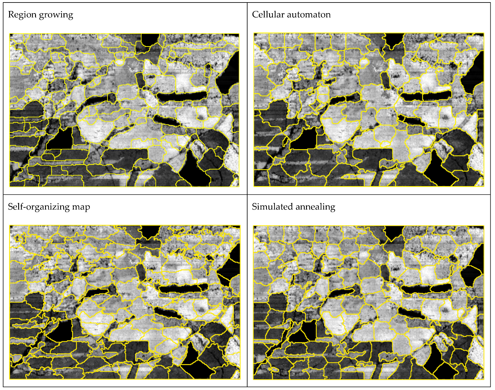
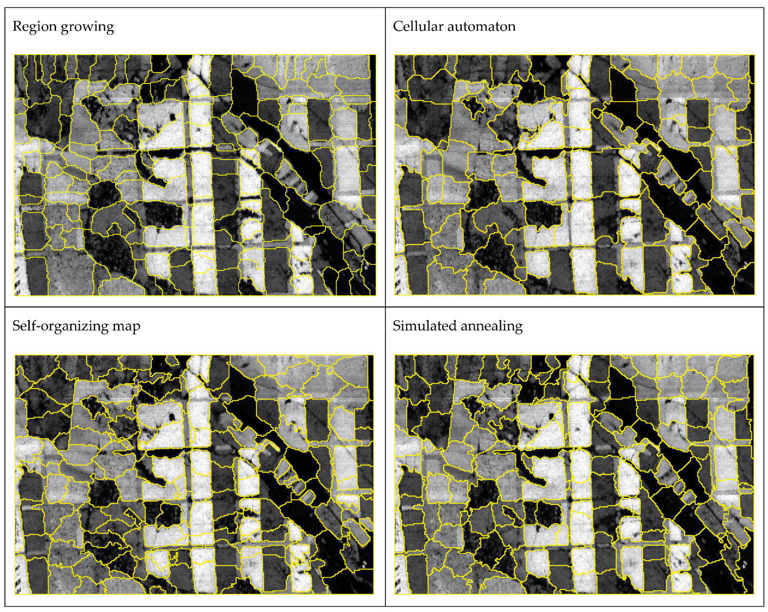
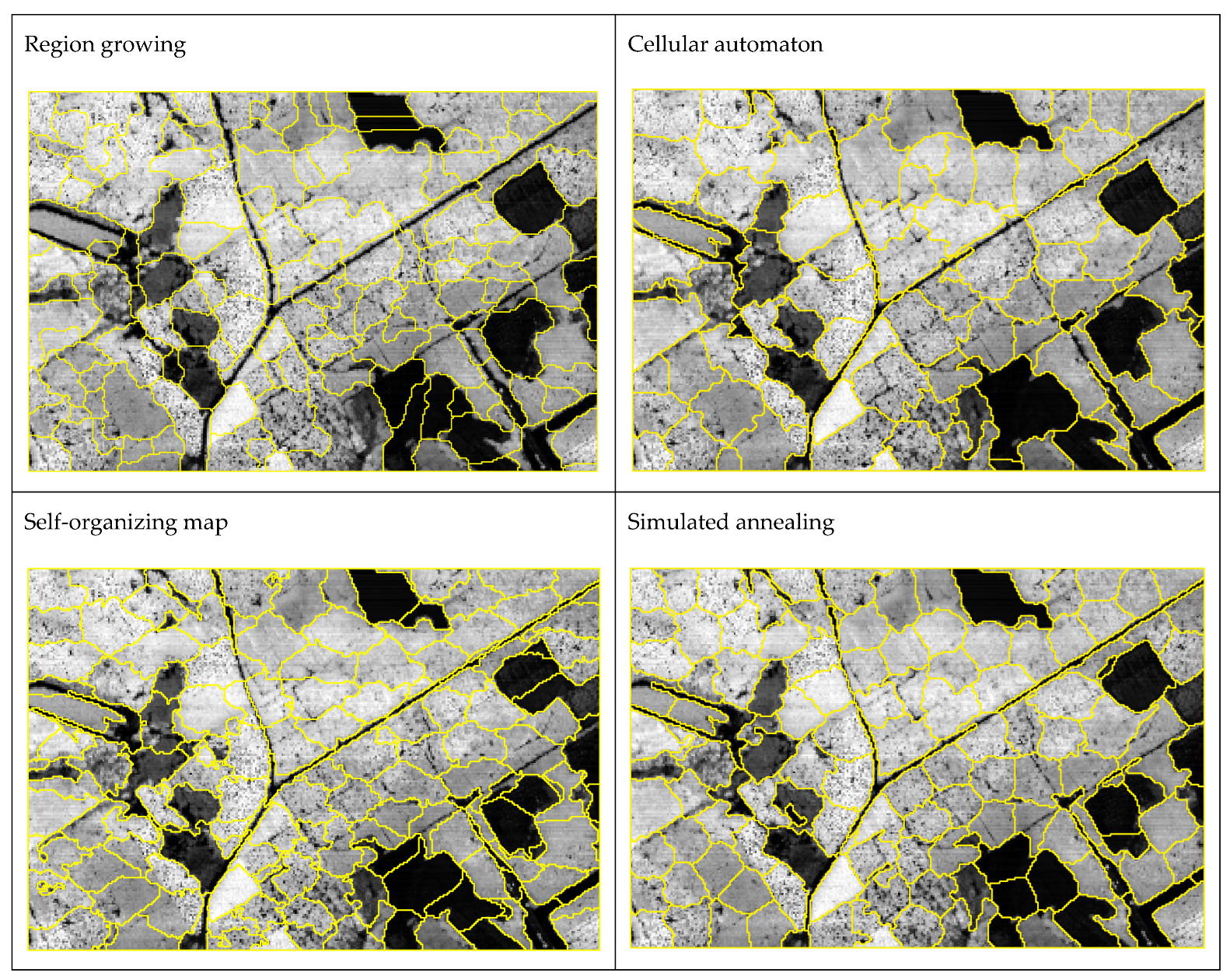
The objective of this study was to compare the performance of the region growing, cellular automaton, self-organizing map, and simulating annealing in automated stand delineation. The purpose was to increase the knowledge and understanding of the potential usability of the new methods. The variables used in the delineation were three metrics calculated from LiDAR scanning data.
2. Materials and Methods
2.1. Study Sites and Field Data
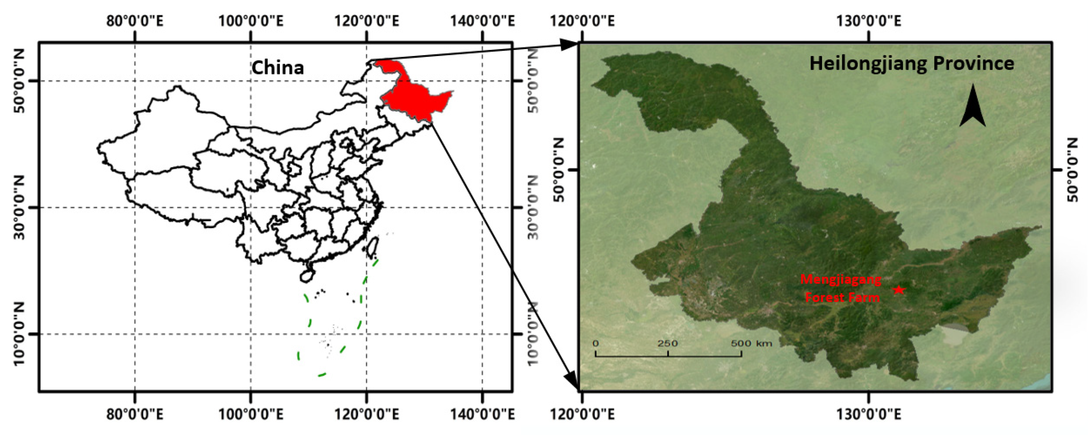
The study area is located in the Mengjiagang forest farm of 15,503 ha, owned by the Huanan country in Heilongjiang Province of China (45°30′16″–46°20′20″N, 130°32′0″–130°52′6″E) (
Figure 1). Most forests are plantations dominated by coniferous tree species, predominantly
Pinus koraiensis,
Pinus sylvestris var.
mongolica,
Larix olgensis, and
Picea asperata. The case study forest has an average elevation of approximately 250 m a.s.l. with a range of 180–450 m. The area is characterized by relatively flat slopes [
20].
2.2. Data Acquisition and LiDAR Metrics
Laser scanning from an unmanned aerial vehicle (UAVLS) was conducted on 12 August 2019, using a RIEGL VUX-1UAV LiDAR scanner (
www.riegl.com/products/unmanned-scanning/rieglminivux-1uav, accessed on 19 October 2022) carried by a DJI M600 Pro unmanned aerial vehicle (eight-rotor UAV platform). The services provided by the RIEGL (RIEGL Laser Measurement Systems GmbH, Horn, Austria) also included basic data processing. The study area consisted of three rectangular 1 km × 1.5 km sub-areas, which were scanned from an altitude of 180 m above ground. The flight speed was 10 m/s. A total of 6 flights were carried out. The laser scanner had a 330° field of view (FOV). The scanning of the three sub-areas lasted for one hour. The maximum point density was 136 pulses/m
2, with up to 5 echoes. The main characteristics of the scanning are summarized in
Table 1.
Before calculating the structural metrics from the UAVLS point cloud data, some data pre-processing was conducted. First, the noise points were removed from the LiDAR point clouds by using a Gaussian-smoothing filter [
21]. Second, a cloth simulation filter was employed to separate non-ground and ground point clouds using parameters 0.5 as the value of the grid resolution, 0.6 as the time step, and 3 as the rigidness [
22]. The average density of ground points was 17 pulses/m
2. Then, the digital elevation model (DEM) was constructed using the ground points and the Kriging interpolation method with a 1 m spatial resolution [
23]. Finally, The UAVLS point clouds were height-normalized by the DEM. The normalized point clouds were clipped with a 1 km × 1.5 km rectangular boundary. Three subareas of this size were used in the study.
A set of UAVLS metrics were calculated for 1 m
2 raster cells using the normalized point cloud data and the LiDAR360 software (
www.lidar360.com). Three categories of metrics were calculated: height-related metrics, intensity-related metrics, and topography-related metrics. Height-related and intensity-related metrics were calculated from the normalized point clouds, and they included the percentiles (1%, 5%, 10%, 20%, 25%h, 30%, 40%, …, 90%, 95%, 99%) of echo heights, cumulative heights, and intensities. Other standard metrics such as the variance, standard deviation, coefficient of variation, skewness, kurtosis, average absolute deviation, mean, maximum and median of the heights, and intensities of the echoes were also calculated [
4]. Topography-related metrics were calculated from the DEM and included the elevation, aspect, and slope of the terrain.
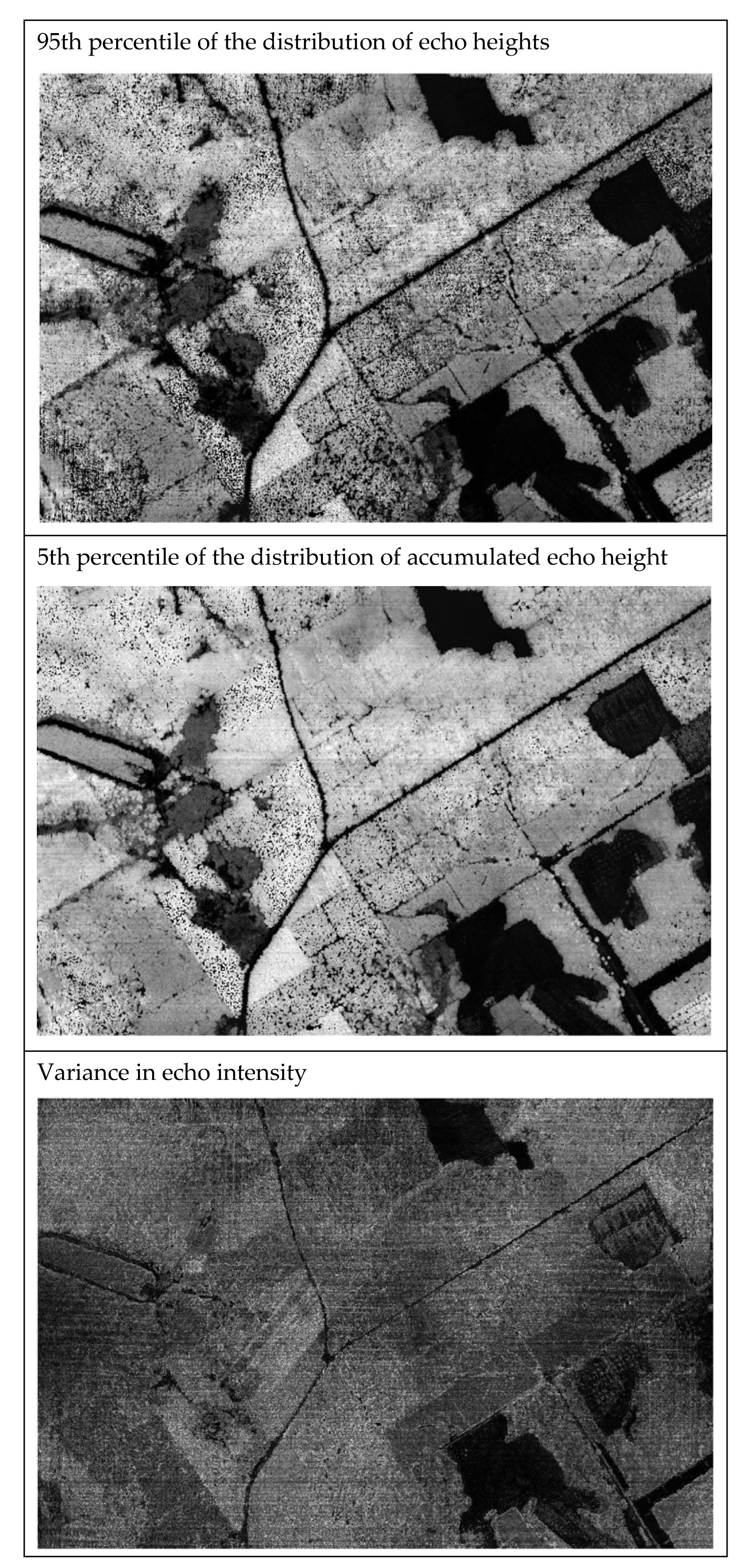
Based on the study of Sun et al. (2021), the following three LiDAR metrics were used in stand lineation (
Figure 2): 95th percentile of the height distribution of normalized echo height (referred to as
HP95), 5th percentile of the accumulated echo heights (
AH5), and variance of the intensity of the echoes (
IV) [
4]. Sun et al. (2021) concluded that while
HP95 is the most important variable for the segmentation, the result would improve if other LiDAR metrics were used as well. Based on Sun et al. (2021), the weights of the three LiDAR metrics were as follows:
HP95: 0.7,
AH5: 0.2, and
IV: 0.1. These weights were used in all four delineation methods tested in this study.
The three LiDAR variables (
HP95,
AH5,
IV) were first calculated for 1 m
2 raster cells. Based on the recommendation of Jia et al. (2020), the 1 m
2 rasters were resampled to a 5 m by 5 m cell size because the use of smaller cells may delineate crowns of individual large trees and produce very rugged segment boundaries [
3]. The metrics of the 5 m by 5 m cells were calculated as the means of the 1 m
2 cells that belonged to the larger 5 × 5 m
2 cell.
2.3. Methods
2.3.1. Region-Growing
Region-growing was performed using the segmentation algorithm introduced by Balasubramanian et al. (2008) and implemented in MATLAB (Mathworks, Inc., Natick, MA, USA) [
24]. Region growing (RG) is the process of aggregating the cells of a grid into larger regions. It first determines initial seeds, which are subsequently enlarged into neighbouring cells following the parameters set for area growth and the stopping criteria of area growth [
25,
26].
The use of region growing started with the generation of initial seeds and the calculation of the mean and standard deviation of the variables used in the process. A recent study by Lee and Cok (1991) uses a vector-based gradient map to guide the growth of the regions [
27]. In this study, a weighted mean of the normalized values of three LiDAR metrics within 5 m
2 raster cells was used in the generation of the gradient map. The weighted mean of the LiDAR metrics was calculated from:
Low gradient values correspond to homogenous regions. To form initial growth seeds, we joined adjacent cells for which the gradient was below the sum of the mean and standard deviation within the seed by using 4-neighborhood connectivity (cells to the east, west, north, and south were considered). Seeds larger than 0.025 ha were retained for subsequent region growth.
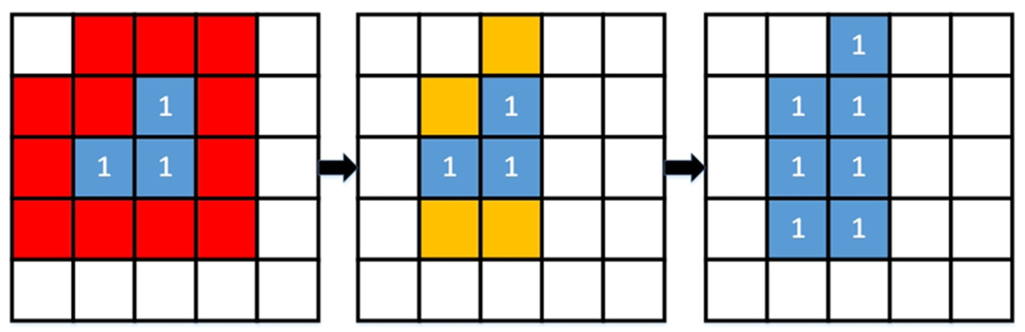
In the region-growing step, the neighbouring cells of a region included the adjacent “side cells” (cells to the east, west, north, and south) and the “corner cells” (cells to the northeast, southeast, southwest, and northwest) of those cells that constituted the region, i.e., 8-neighbourhood was used (
Figure 3). The initial growth seeds expanded toward neighbouring cells based on a pre-defined homogeneity criterion. The homogeneity criterion employed the vector-based gradient map [
2]. The mean (
m) and standard deviation (σ) computed for each initial growth seed were used to calculate the confidence interval for
C (Equation (1)). If the value of variable
C in the neighboring cell was between
m − σ and
m + σ, the neighboring cell was added to the growing seed and the neighboring cell was given the same segment number as the seed.
The expanding process was stopped when no cells were found that met the joining criterion. To obtain a segment number for all cells, the process was repeated for several iterations. At each iteration, the mean and standard deviation were calculated for the expanded regions, which were subsequently used as the initial growth seeds for the next iteration. The above steps were repeated until each cell belonged to a region (i.e., had a segment number).
2.3.2. Cellular Automaton
The cellular automaton used in this study is the same as that described by Jia et al. (2020) [
3]. The idea of the method is to join each cell of a raster to one of its adjoining segments using the following formula for selecting the most suitable segment for the cell:
where
Pij is the priority, or score, if cell
i is joined to segment
j,
Dij is the Euclidean distance of the LiDAR metrics between cell
i and segment
j,
Aj is the area of segment
j,
Bij is the proportion of the common border between cell
i and segment
j (of the total border length of cell
i),
Sij is the effect of joining cell
i to segment
j on the shape of segment
j,
pk is the sub-priority function for criterion
k, and
wk is the weight of criterion
k. The sum of the weights was equal to one. The score was calculated for each segment adjacent to cell
i, and the number of the segment with the highest score was given to cell
i. When calculating the border length, it was assumed that the side cells to the east, west, south, and north have a length equal to 1 and the corner cells (to the northeast, southeast, southwest and northwest) have a “length” equal to 0.3.
The initial segments were obtained by dividing the area into square-shaped areas. Then, the segment number of each cell of the grid was determined by using Equation (2). This process was repeated for several iterations.
Compared to the first version of the cellular automaton [
8], Jia et al. (2020) introduced a shape metric that affected the assignment of segment numbers for the cells [
3]. The shape metric was based on the distance of the cells of a segment to the segment’s center. Minimizing this distance produces roundish segments without long and narrow extensions.
All four criteria used in Equation (2) had an associated sub-priority function, which determined the effect of segment area, common border, segment shape, and difference in LiDAR metrics between the cell and the segment on the sub-priority obtained from the criterion. We used the same sub-priority functions as Jia et al. (2020) [
3]. As shown by Equation (2), the sub-priorities were multiplied by the criteria weights and summed.
The difference between LiDAR metrics in cell
i and segment
j was calculated from the normalized values of the metrics as follows:
where
J is the number of segments adjacent to cell
i. The sub-priority was inversely proportional to the difference, i.e., a smaller difference in the LiDAR metrics between cell
i and segment
j increased the probability that cell
i was joined to segment
j. Since all LiDAR metrics were scaled to the range 0–1, the sub-priority also ranged from 0 to 1.
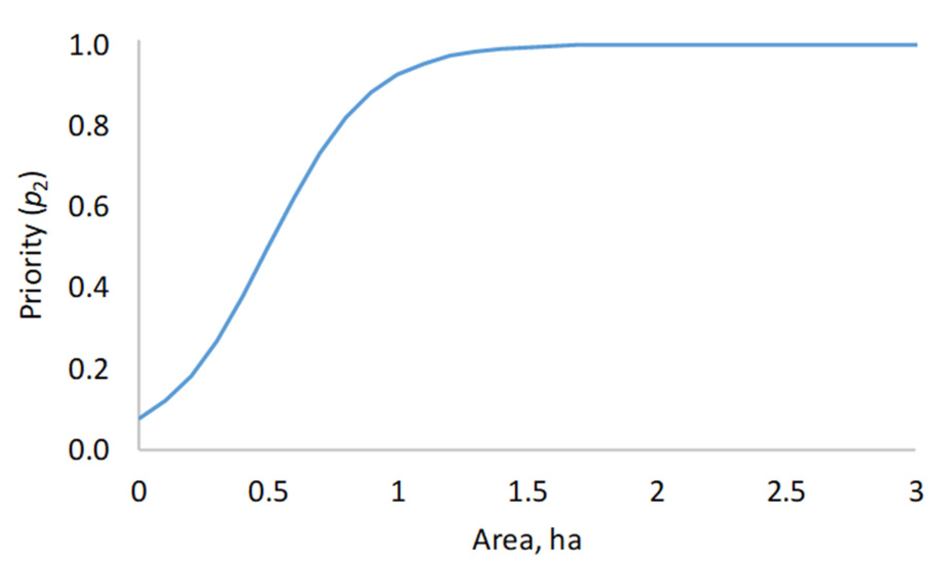
The sub-priority functions for the segment area and the common border between the cell and a segment were logistic curves, which resulted in sub-priorities ranging from zero to one. For example, the sub-priority function for the segment area was:
where
Aj is the area of segment
j in hectares. The sub-priority function is graphically depicted in
Figure 4. It indicates that increasing the segment area increases the likelihood that a cell is joined to the segment, but the effect is almost over at about 1.5 hectares. As a result of the shape of the sub-priority function (
Figure 4), the cellular automaton avoids joining cells to segments whose area is clearly less than one hectare. However, other criteria of the priority function (Equation (2)) may favour a small segment, which means that small segments are not ruled out completely.
2.3.3. Self-Organizing Map
The variant of the self-organizing map adapted to stand delineation by Pukkala (2021) was used in this study [
9,
19]. The algorithm begins with the creation of initial neurons. In Pukkala’s (2021) study as well as in ours, the initial neurons were obtained by dividing the area into squares (for instance, 1 ha squares) and calculating the mean values of the normalized LiDAR metrics and the
x and
y coordinates for each square [
9]. Each neuron was associated with the values of
HP95,
AH5,
IV,
x coordinate, and
y coordinate.
Then, a training process was initiated that consisted of selecting a random cell from the grid and finding the neuron most similar to it in terms of the five variables listed above (
HP95,
AH5,
IV,
x,
y). The similarity was assessed by using the weighted Euclidean distance
where
Dij is the distance between cell
i and neuron
j, and
v is the weight of coordinates. Before calculating the distance, all variables were normalized to a mean of zero and a standard deviation of one.
The neuron that is most similar to cell
i is called the best matching unit (BMU). The attribute values (
HP95,
AH5,
IV,
x,
y) of the BMU were updated using
where
zjk is the value of attribute
k in neuron
j,
zik is the value of the same attribute in cell
i,
t is the number of the current iteration and α(
t) is the learning rate. The initial value of the learning rate parameter was 1, and it was updated after every iteration as follows
The number of training iterations (tMax) was 10000, which means that the process of selecting a random cell, finding the BMU for it, and updating the attribute values of the BMU was repeated 10,000 times. Then, classification was performed where each cell of the raster was linked to the neuron most similar to it in terms of Euclidean distance (Equation (5)). The number of the most similar neuron was given to the cell. Due to the use of coordinates, cells that constituted a class were usually adjacent, and the classes could therefore be interpreted to be segments.
As suggested by Pukkala (2021), the process that consisted of the production of initial neurons, training, and classification was repeated a few more times (10 times in this study) [
9]. In the second and all later repetitions, the attribute values of initial neurons were obtained from the means of the classes of the previous classification. However, classes that had only a few cells were discarded, which means that the number of initial neurons may decrease when the self-organization process is repeated. In this study, all classes (segments) smaller than 0.1 ha were discarded at the beginning of a new self-organization round.
2.3.4. Simulated Annealing
In the same way, as in cellular automaton, simulated annealing (SA) was started by dividing the area into square-shaped initial segments [
4]. In the SA method, these segments are called the initial solution. Then, a random cell was selected from the grid. If this cell was located at the segment border (at least one of its adjacent cells belonged to a different segment), the possibility to change the segment number of the cell was considered. The choice depended on the effect of the change on the properties of the segment to which it would be joined (recipient segment) and the current segment of the cell (donor segment). In SA, changing the segment number of a raster cell was called a move.
The formula that was used to evaluate the effect of the move was as follows:
The formula expresses the quality of the segment as a function of three criteria: segment area (
A), variance of the LiDAR metrics (
HP95,
AH5,
IV) within the segment (
V), and shape of the segment (
S). The quality measure was calculated for both the donor and the recipient segment before and after implementing the move. If the move improved the average quality score of the two segments, it was accepted. Otherwise, the move was accepted with the following probability (
p):
where
QBefore is the average quality score of the two segments before the move and
QAfter is the average score if the move is implemented.
T is a “temperature” parameter that affects the probability of implementing inferior moves. The temperature parameter had a starting value and an ending value (“freezing temperature”). At each temperature, a certain number of candidate moves were produced and evaluated, after which the temperature was multiplied by a constant smaller than one. The process was terminated when the temperature reached freezing temperature.
In this study, the number of candidate moves (random cells) evaluated at each temperature was 50,000. This number also includes those randomly selected cells that were not located at the segment border and were therefore not eligible for a move. The initial temperature was 0.1, the freezing temperature was 0.0001, and the multiplier to obtain a new temperature was 0.95. These parameters are based on the analyses of Sun et al. (2021) [
4].
In Equation (8), which was used to evaluate the quality of a segment, the sub-priority function for segment area was the same as used in cellular automaton (
Figure 4). The sub-priority function for within-segment variance (
V) was
where
V is the weighted mean of the relative variances of
HP95,
AH5, and
IV within the segment. The formula implies that the quality score from variance decreases with increasing within-segment variation in
HP95,
AH5, and
IV. The relative variance was calculated by dividing the variance of the cell values by the mean value of the attribute within the segment. The weighted mean of the relative variances (
RV) was calculated from
The priority function for segment shape was the one suggested by Sun et al. (2021) [
4]. It is different from the one used in the cellular automaton, although in both cases the idea of the shape metric is to measure deviation from a circular shape. The quality points from the segment shape were calculated as follows:
where
n is the number of cells that belong to the segment and
RDi is the relative distance of cell
i from the segment centroid.
RD was calculated by dividing the distance by the radius of a circle that has the same area as the segment. The shape score of the segment is calculated as the mean of cell-level distance scores.
2.4. Post-Processing
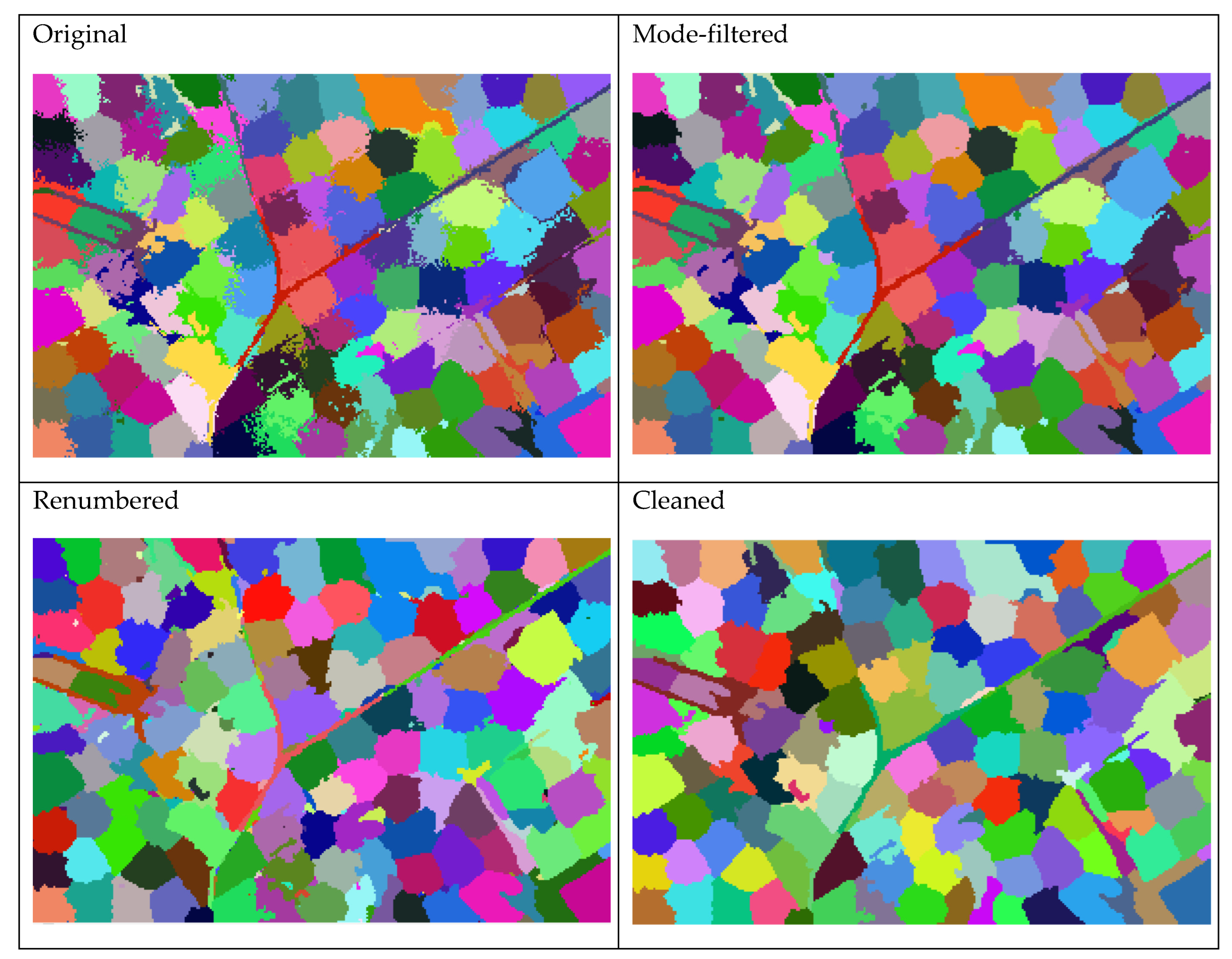
All three methods tested as alternatives for region growing (CA, SOM, SA) may split segments into disconnected parts. The methods may also produce rugged boundaries and result in a gradual change in stand number (
Figure 5 top left). These outcomes are more common in SOM and SA as compared to CA [
3,
4,
9]. Although the delineations obtained from the algorithms correspond to the spatial variation of the attribute values within the input raster, divided segments, gradual changes, and rugged segment boundaries may not be appreciated in forestry practice. In addition, very small segments are seldom desired as forest management units since they make it difficult to implement treatments.
To mitigate these problems, the segmentations obtained from CA, SOM, and SA were post-processed in three steps. First, a mode filter with a 3 × 3 cell window was applied to the segmentation: the segment number of every cell was replaced by the most common segment number of the 9-cell window. This process smoothed segment boundaries and reduced gradual transitions (
Figure 5, top left and top right).
Second, non-connected parts of segments were given different segment numbers, i.e., they were interpreted to be different segments (
Figure 5, bottom left). Third, another model filter was applied to cells that belonged to segments smaller than 0.1 ha. The segment number of these cells was replaced by the most common segment number within a 9 × 9 cell window. This post-processing step was called cleaning (
Figure 5, bottom right).
Of these post-processing steps, mode filtering increases the within-segment variation in LiDAR metrics and renumbering decreases it. However, the effects are usually small [
4]. Both mode-filtering and renumbering tend to improve the shapes of the segments [
21]. Renumbering decreases the average area points of the stands as it creates new small segments, and cleaning has the opposite effect.
2.5. Fine-Tuning of CA, SOM, and SA
Most of the parameters of CA, SOM, and SA were taken from previous studies [
3,
4,
9], which have analyzed the effects of parameters on the segmentation results and recommended certain parameter values. However, additional sensitivity analyses were conducted to find the most suitable size of initial stands and suitable weights for the quality criteria of the segments.
Three different sizes of the square-shaped initial stands were compared within each method (CA, SOM, SA): 1 ha, 1.5 ha, and 2 ha. In addition, three different sets of criteria weights were tested. In CA, the weight of Euclidean distance between a cell and a segment (criterion D in Equation (2)) was 0.1, 0.4, or 0.7, and the weights of the three other criteria (area, shape, common border) were equal (0.3, 0.2, or 0.1). This resulted in nine combinations of initial segment area and criteria weights.
In SOM, each initial segment area was tested with three different weights of coordinates in Equation (5). Equation (5) was used to measure the similarity between a cell and a neuron. The weight of the coordinates was 3, 6, or 9 while the weights of HP95, AH5, and IV were always 0.7, 0.2, and 0.1, respectively. An increasing weight of coordinates results in more compact, roundish, and even-sized segments.
In SA, the criteria weights of Equation (8) were modified so that the weight of within-segment variance was 0.5, 0.7, or 0.9. The weights of the other criteria (area and shape) were equal in such a way that the sum of the three weights was always 1.
2.6. Statistics Calculated for the Segmentations
The delineations produced by the four methods were evaluated by calculating the degree of the variance in
HP95,
AH5, and
IV which was explained by the delineation (R
2). The R
2 statistic was calculated from
where SSE is the variation not explained by the delineation and SST is the total variation of the attribute within the grid. SST and SSE were calculated as follows:
where
N is the number of segments,
nj is the number of cells in segment
j,
zij is the value of the attribute (
HP95,
AH5 or
IV) in cell
i of segment
j,
is the overall mean of the attribute, and
is the mean value of the attribute among the cells that belong to segment
j.
In addition, the average segment area and the proportion of segments smaller than 0.3 ha were calculated for each segmentation. The shape of the segments was assessed using metrics that measure deviation from a circular shape. First, a radius of a circle having the same area as the segment was calculated for each segment. Then, the average distance of the cells from the segment center was calculated, using the length of the radius as the unit. For example, if the segment area is 1.2 ha, it corresponds to a 61.8-m radius. If the average distance of the cells from the segment’s center is 45 m, it corresponds to a relative distance of 0.727 (45/61.8 = 0.728, i.e., 0.728 radii from the center). The centre of the segment was defined by the mean x and y coordinates of the cells that constituted the segment.
In addition, the proportion of cells that were within one radius of the segment center was calculated for each segment. Then, the average distance and average proportion of cells within one radius were calculated over all segments. These averages were calculated with and without using segment area as the weight variable.
4. Discussion
To increase the knowledge and understanding of the potential usability of alternative methods proposed for automated stand delineation, this study analyzed the performance of four different segmentation algorithms, analyzed using LiDAR metrics calculated for 5 m by 5 m raster cells as the data source. The study showed that all the segmentation methods can be used to segment forests into stands when LiDAR scanning data are available. Laser scanning can capture such characteristics of forest canopies that are essential for delineating stands in large areas [
28].
All the automated segmentation methods tested in this study provide feasible options for stand delineation in the context of forest management, especially in plantations. Our study corroborated the results of several recent studies [
3,
4,
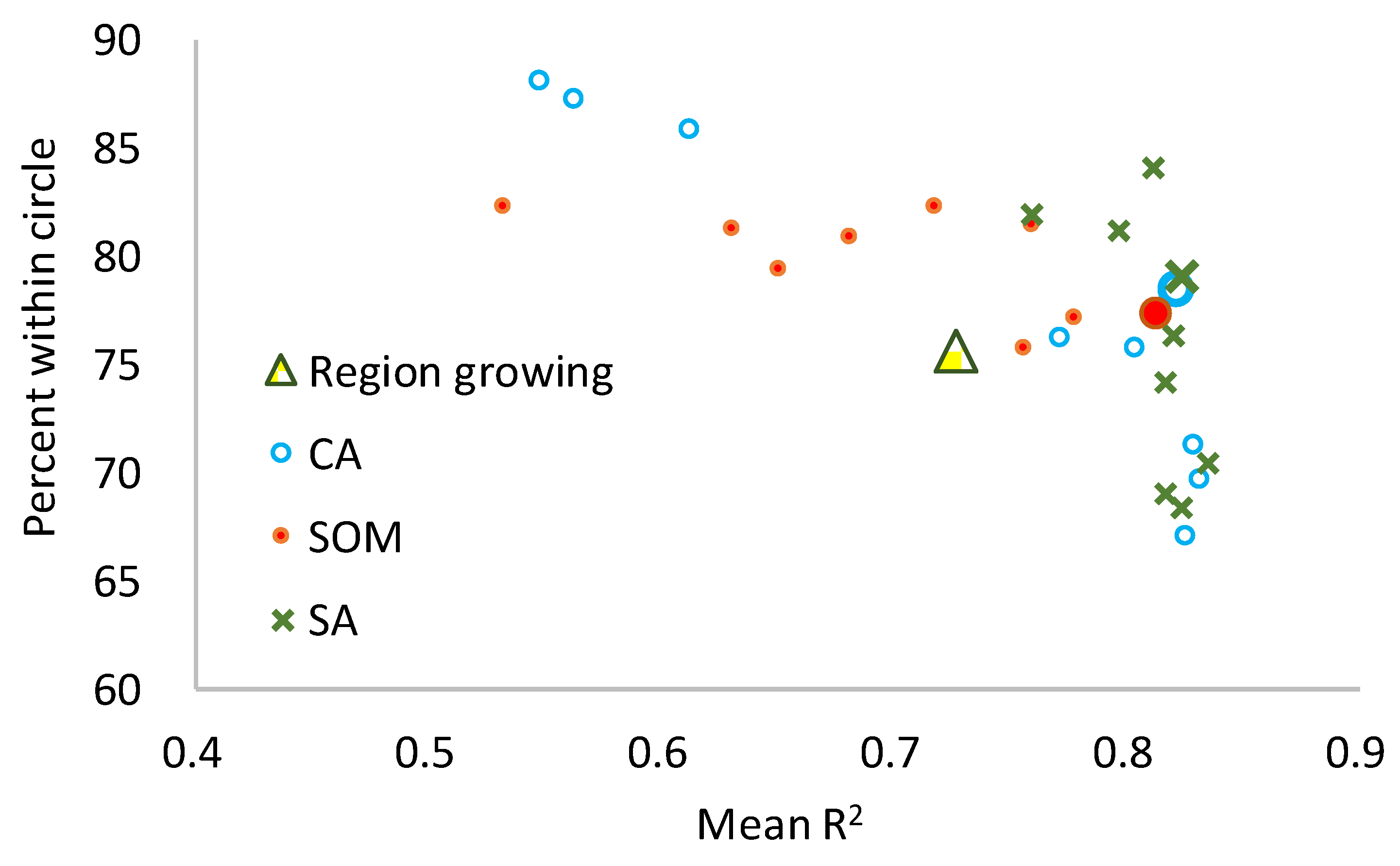
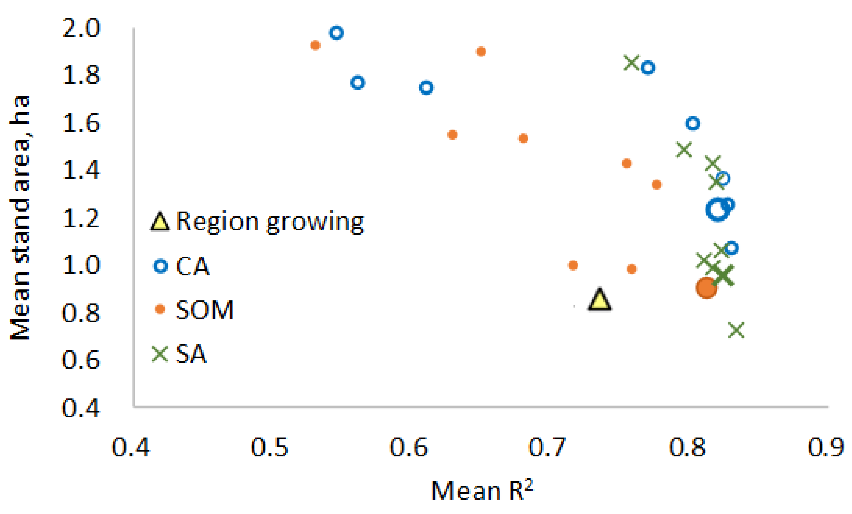
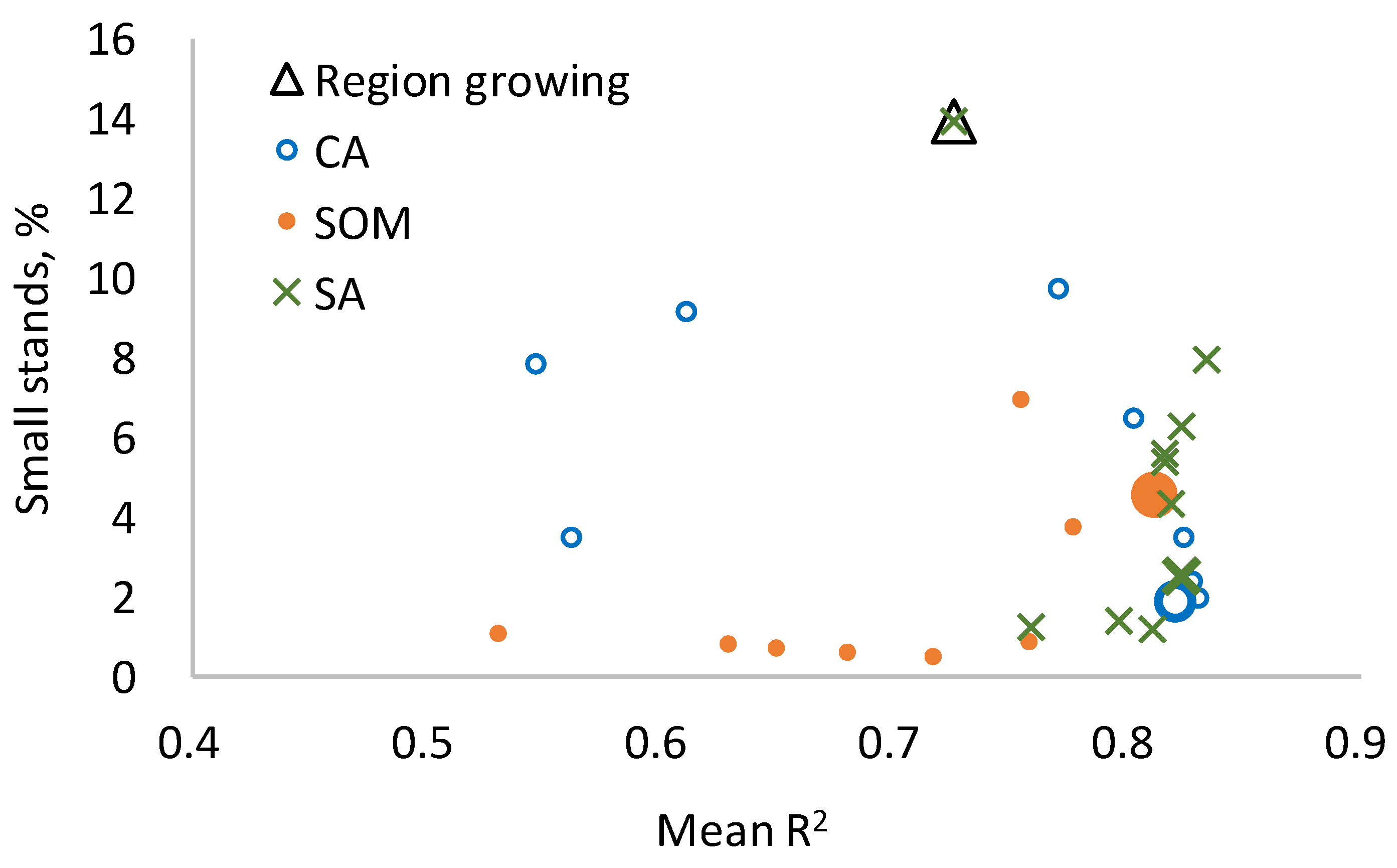
9]. In the analyses of this study, however, CA, SOM, and SA outperformed the region-growing method since they produced more homogeneous segments than region-growing. For wider generalization, this result needs to be confirmed in other types of forests and datasets.
The algorithms used in this study are easy to implement in computer programs. In this respect, the SOM might be the easiest one (see the meta code provided in Pukkala, 2021) [
9]. It is also the fastest method to use. The simulated annealing algorithm needs much longer times to run, the cellular automaton being between SOM and SA. On the other hand,
Table 2,
Table 3 and
Table 4 suggest that the delineations produced by the SA method may be evaluated to be slightly better than those obtained from CA and SOM.
We used 25 m
2 raster cells of three UAVLS variables to segment the forest, which together represent most of the information contained in the nearly 90 LiDAR metrics calculated for the raster cells [
4]. Sun et al. (2022) also suggested that the use of a fourth metric, namely, a texture variable describing the variation of
HP95 within the 5 m × 5 m raster, might be useful [
21]. This possibility was also checked in the current study, and it was found that texture varied significantly only in one of the three sub-areas. The contribution of the texture variable to the delineation result would have remained small in the other sub-areas.
Increasing the initial stand area had a clear effect on the delineation result. Because SOM, SA, and CA methods cannot produce new segments (new segment numbers) but segments may disappear during the segmentation process, small initial segments usually lead to better results than the use of large initial segments. However, the conclusion might be different if renumbering is applied during the segmentation run [
3]. Renumbering means that disconnected parts of the segments are given different stand numbers. We did not implement this possibility during the CA, SOM, and SA runs (but only afterwards) because we wanted to compare the basic versions of these methods to the region-growing algorithm. Renumbering during the segmentation process can be expected to improve the performance of the methods, and it makes the algorithms less dependent on the initial segment area.
In the present study, the region-growing method was the poorest of the four tested segmentation methods, especially in terms of R2. Region growing was more competitive in the stand area and shape statistics, although these variables were not used as criteria in the region-growing algorithm. Perhaps the fact that the segment area was not used as a criterion was the reason why the number of small segments (< 0.3 ha) was higher in RG than in the other methods. On the other hand, the region-growing method can prevent the creation of small stands simply by setting a large enough minimum size for the initial growth seeds.
The use of very small initial segments may also be harmful since several adjacent initial segments may be demarcated within the same large homogeneous stand. Some of the methods, especially CA, do not move the initial segment boundaries easily in a homogeneous region, resulting in segmentations where large stands are unnecessarily divided into several small segments. This shortcoming could be mitigated by increasing the weight of the area criterion and modifying its priority function. Based on our study, it may be concluded that the optimal initial stand size is around 1 ha when UAVLS data are used for stand delineation in the forests of Heilongjiang province.
CA differs from the other methods in such a way that the common border between a cell and the adjacent segments is taken into account. Therefore, the method often leads to smoother stand boundaries than SA and SOM [
4,
7]. On the other hand, rugged stand borders can easily be smoothed afterward by using mode filtering.
The main objective of stand delineation is to find a balance between a low within-stand variation and suitable stand size and regular stand shape. In most cases, the forest managers require that the stands are homogeneous, the stand shape is regular, and the stand boundaries are smooth.
If the delineation criteria emphasize too much low within-stand variation, the result might be unsatisfactory in terms of stand size and shape. There are no official standards for stand delineation as the requirements depend on the preferences of the forest manager and the purpose of the delineation. For example, some forest managers focus on creating larger size segments that correspond to traditional stand compartments, while another possibility would be to create smaller segments for a more accurate prediction of the development of the forest [
13,
21]. Modern forest planning methods make it possible to aggregate small stands used in calculations into larger continuous treatment units [
8,
29]. Regarding the capability of modern forest planning methods, a large number of small homogeneous stands is a better option than a low number of large and less homogeneous stands [
8].
Our study indicated that all segmentation methods were capable of producing good stand delineations in homogeneous plantation forests. Failures are more likely to happen in natural forests that are often spatially heterogeneous with small trees occurring in the gaps of a higher canopy. As discussed in Pukkala (2021), SOM has the advantage that it can divide a heterogeneous forest into two or more overlapping sub-stands, one for the small trees or canopy gaps and the other for areas of taller trees [
9]. The overlapping stands may consist of several disconnected parts. This feature of the SOM may also be useful in retention forestry where groups of retention trees are left in regeneration areas. Delineating all groups of retention trees as different stands may not be an ideal solution as the groups can be very small.
Additional possibilities to improve the delineation of heterogeneous forests into stands would be to use K-means clustering or other similar methods to create the initial segments for the CA, SOM, and SA methods [
30]. This would mitigate the problem that some methods may unnecessarily split large stands into several small segments when a systematic layout of small squares is used as initial stands.
In Chinese forest management, it is not permitted to change the boundaries of forest compartments. This increases the need for delineating compartments that are useful for forest management for long periods. Currently, the Chinese compartment demarcation uses topographic and land type data and can therefore distinguish the forest and non-forest. The methods analyzed in this study could also make use of additional layers, one of which could mask off cells that represent non-forest land uses [
8,
11,
31]. When compartments are large and permanent, it might be worthwhile to repeat the segmentation separately for each compartment. This would make it possible to deal with within-compartment heterogeneity in the simulation of forest development.
LiDAR has a restricted spectral resolution, generally covering a single spectral range in the near-infrared region, which may not be optimal for the interpretation of species composition [
32]. Therefore, new studies should be conducted on integrating multi-source remote sensing data for improved stand delineation. Hyperspectral data may be particularly useful in mixed forests to characterize the tree species composition [
33], biochemical features [
34], and some biophysical properties such as the leaf area index (LAI) and biomass [
35].


