
Assessment of Tropical Cyclone Risk to Coral Reefs: Case Study for Australia
Abstract
:1. Introduction
2. Data and Methods
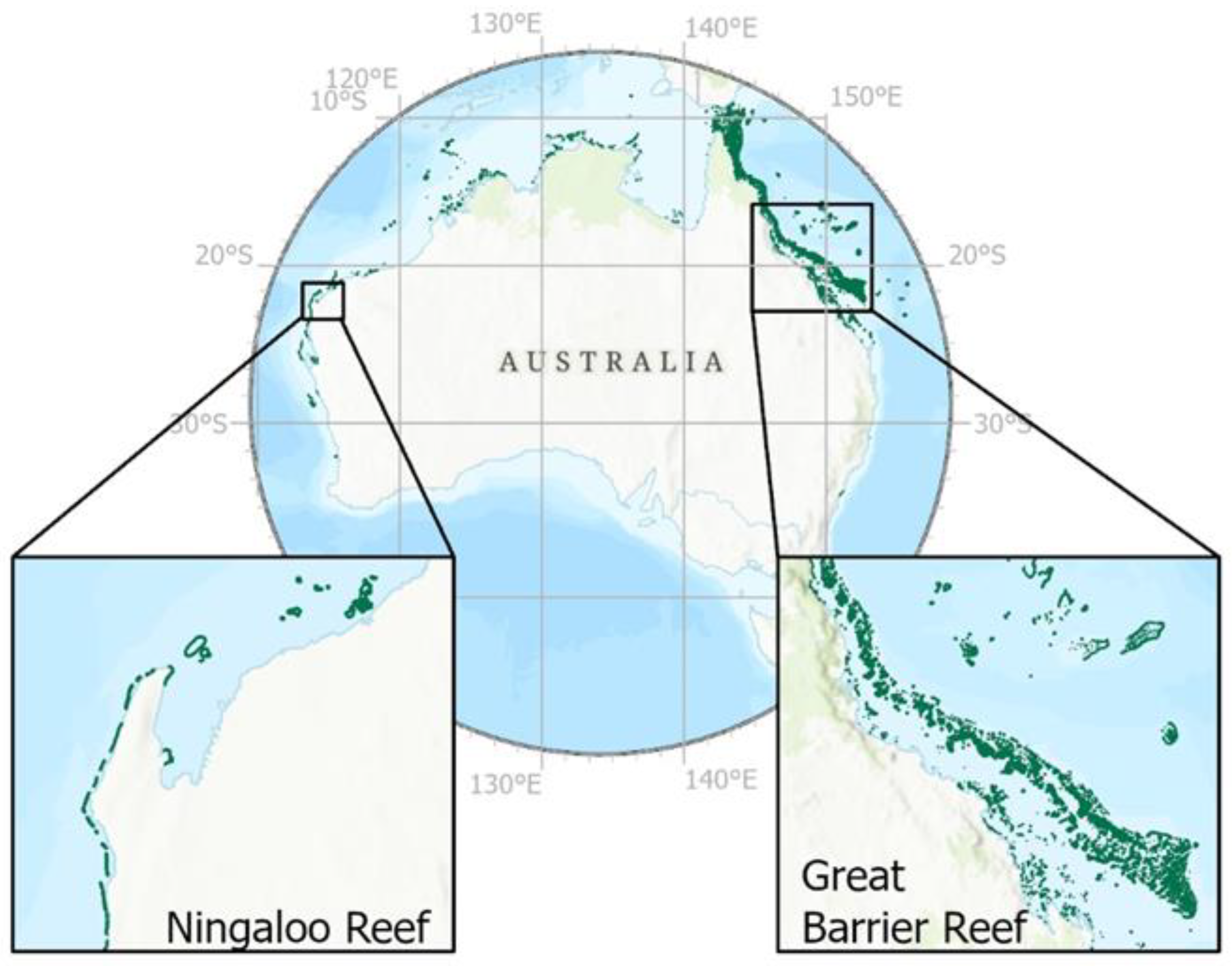
2.1. Study Area
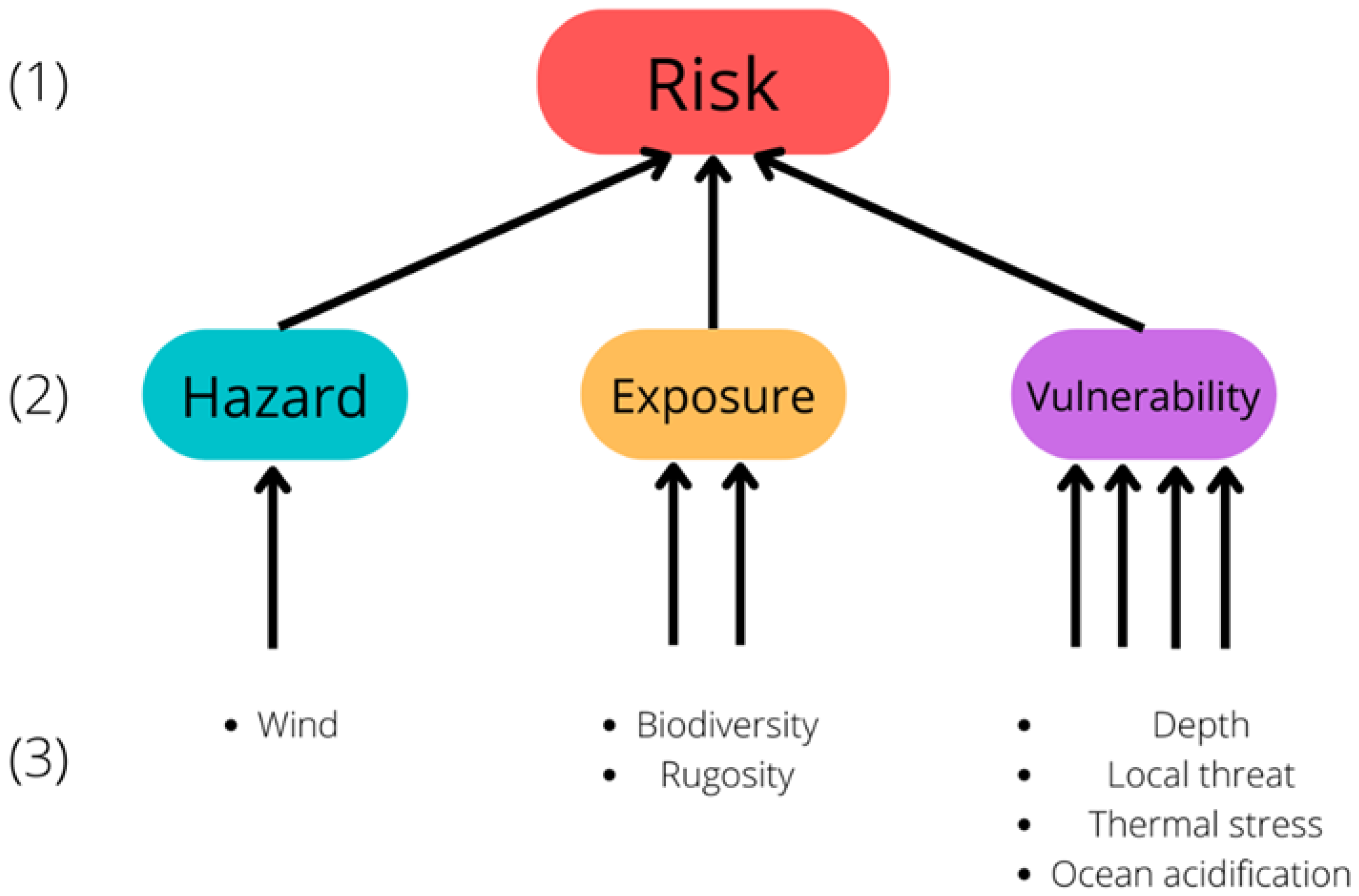
2.2. Definition of Risk
2.3. Selection of Indicators
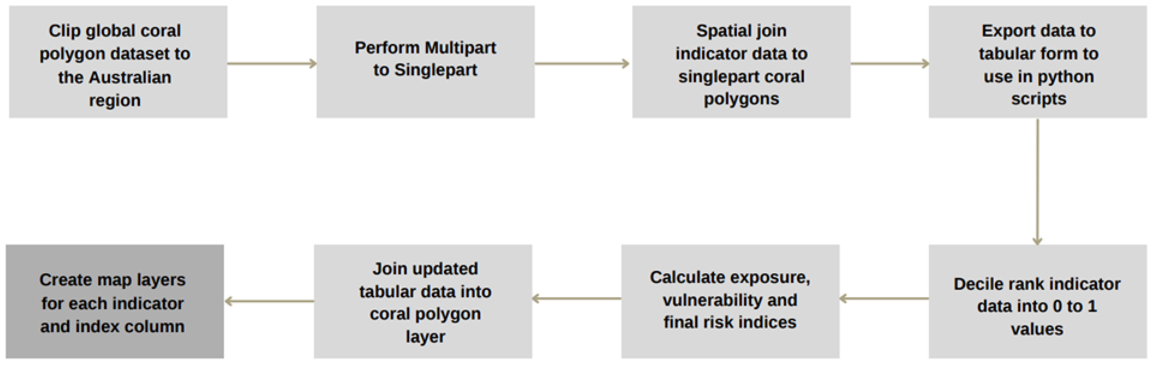
2.4. Methodology for Assessment of TC Risk to Corals
3. Results and Discussion
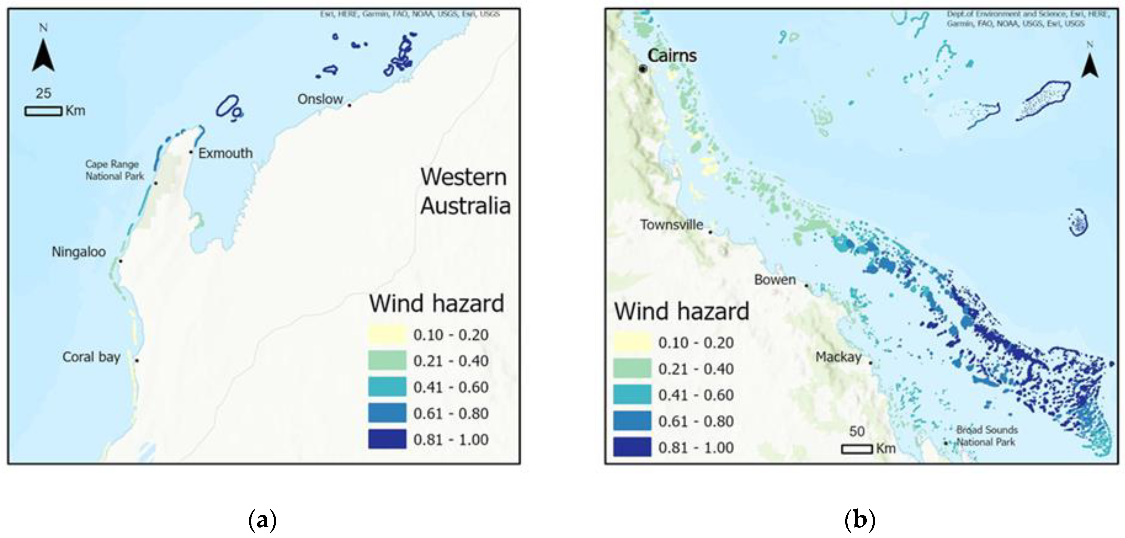
3.1. Hazard
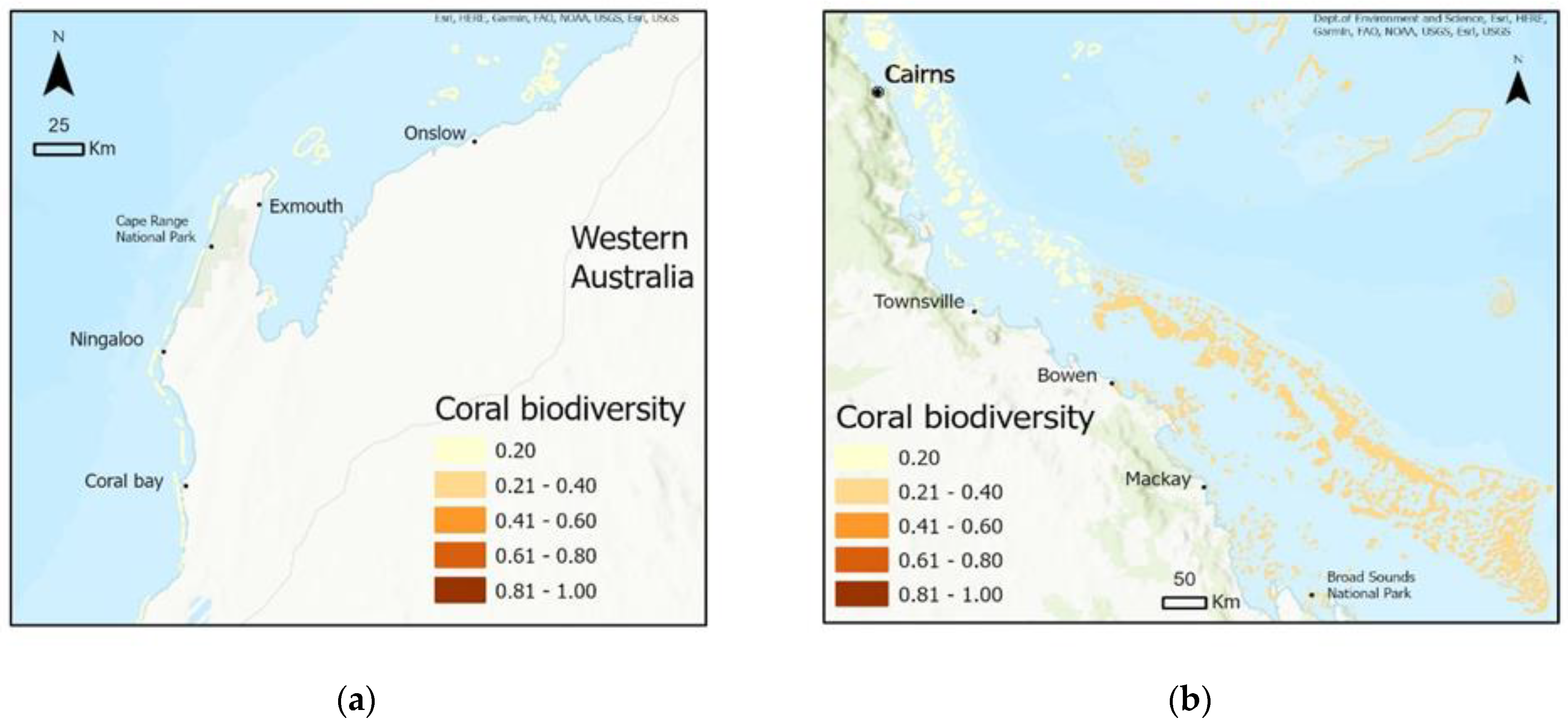
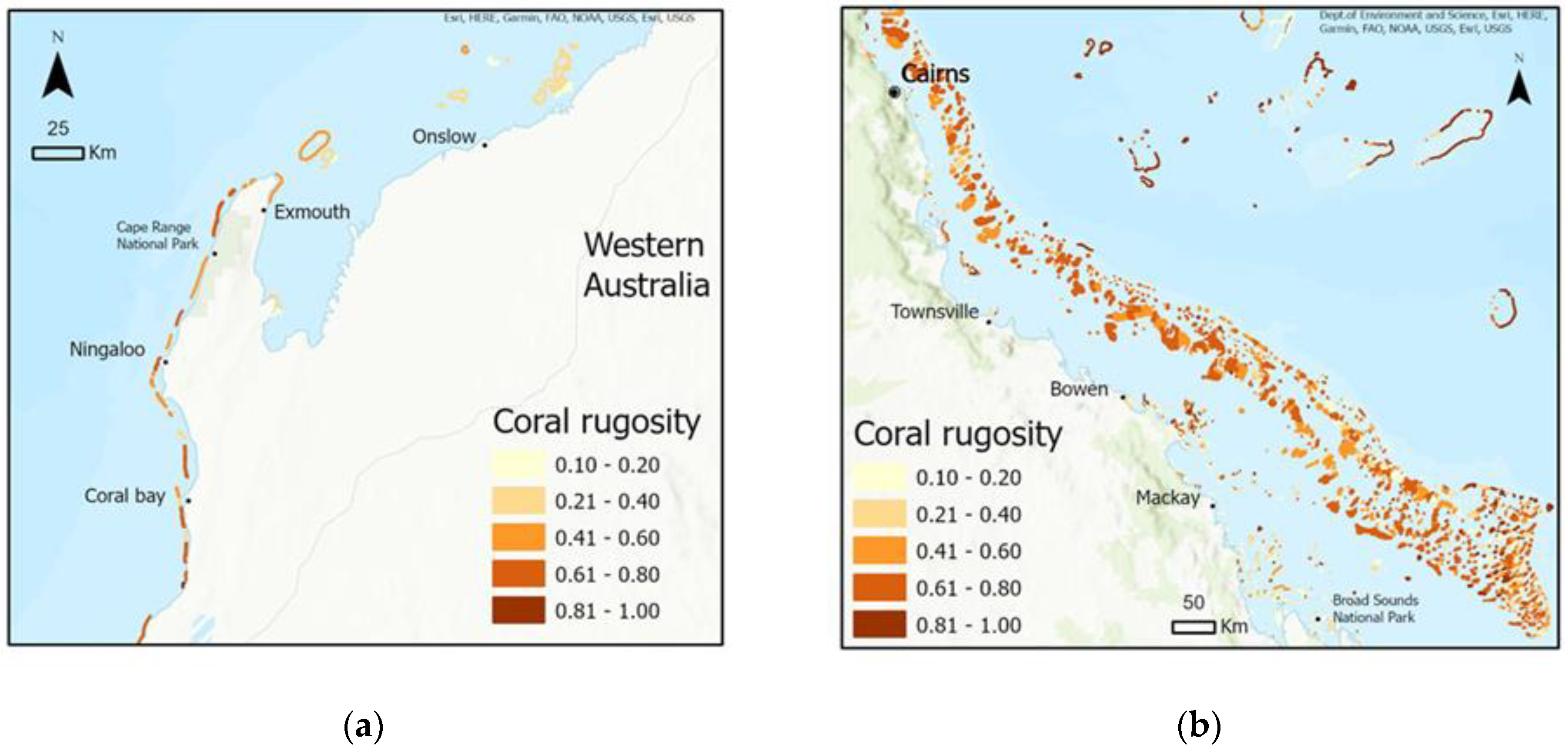
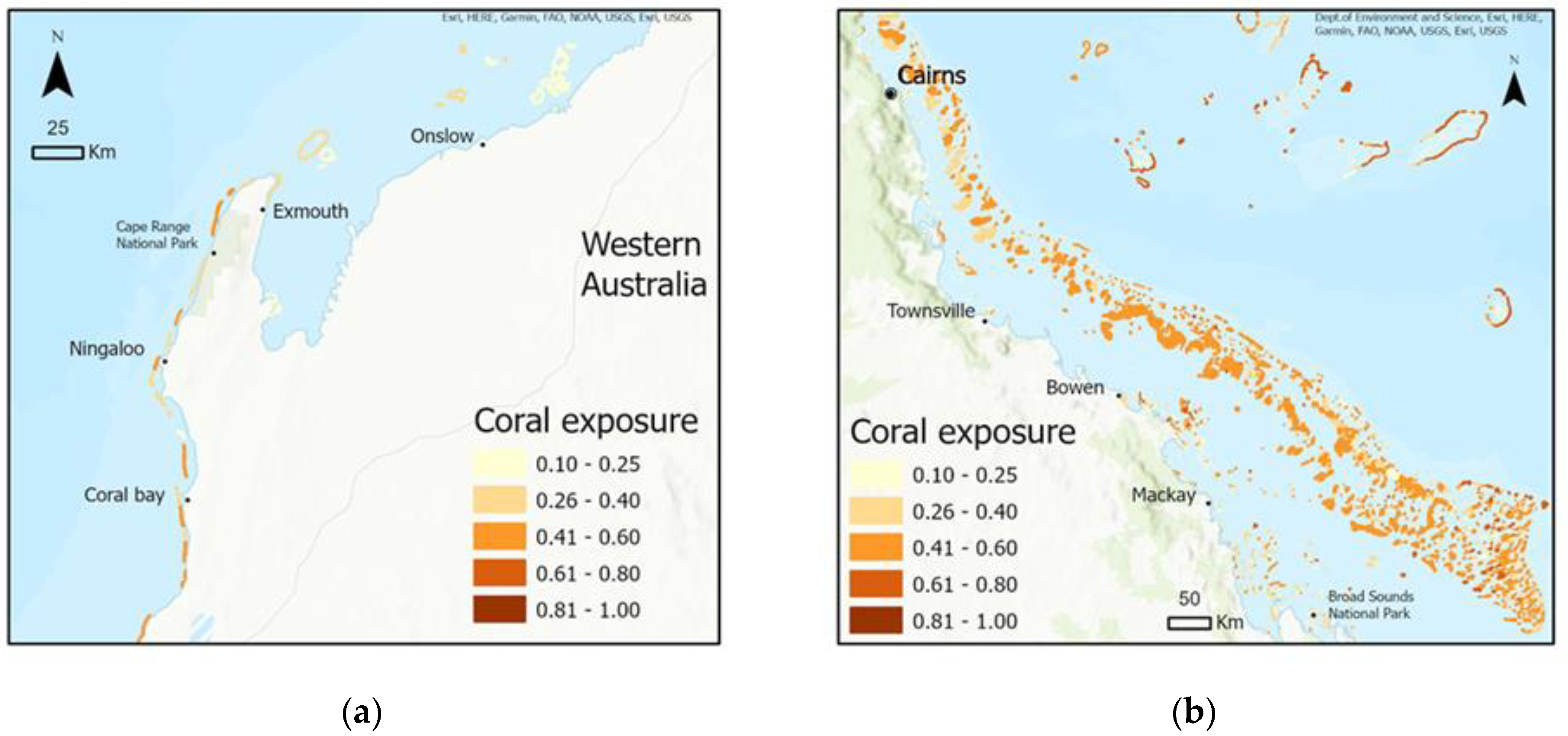
3.2. Exposure
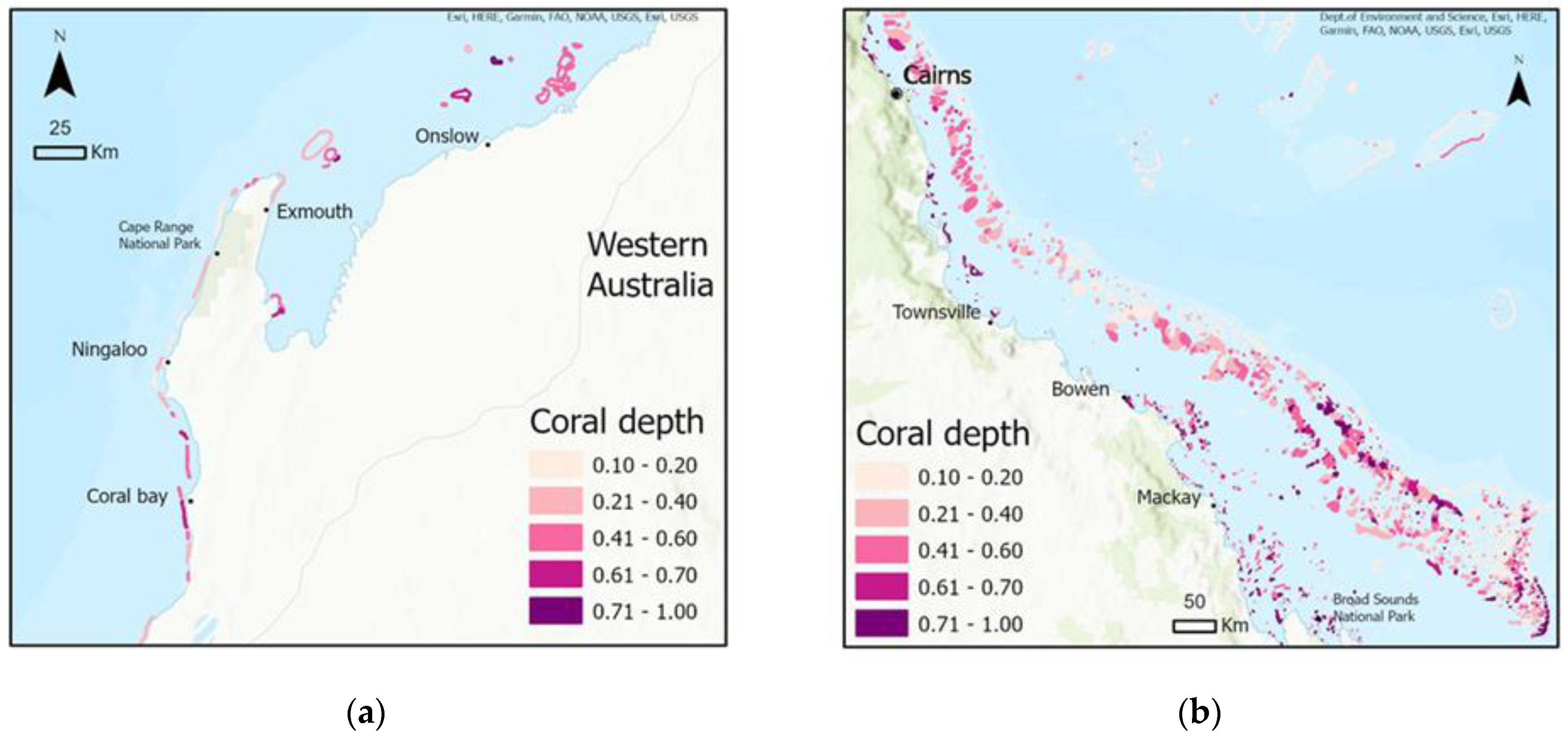
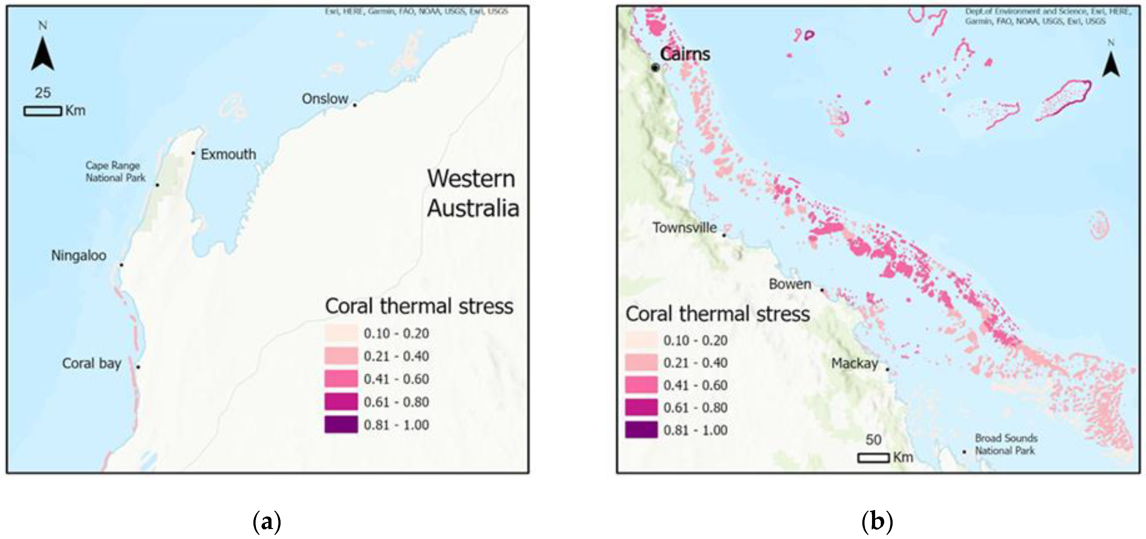
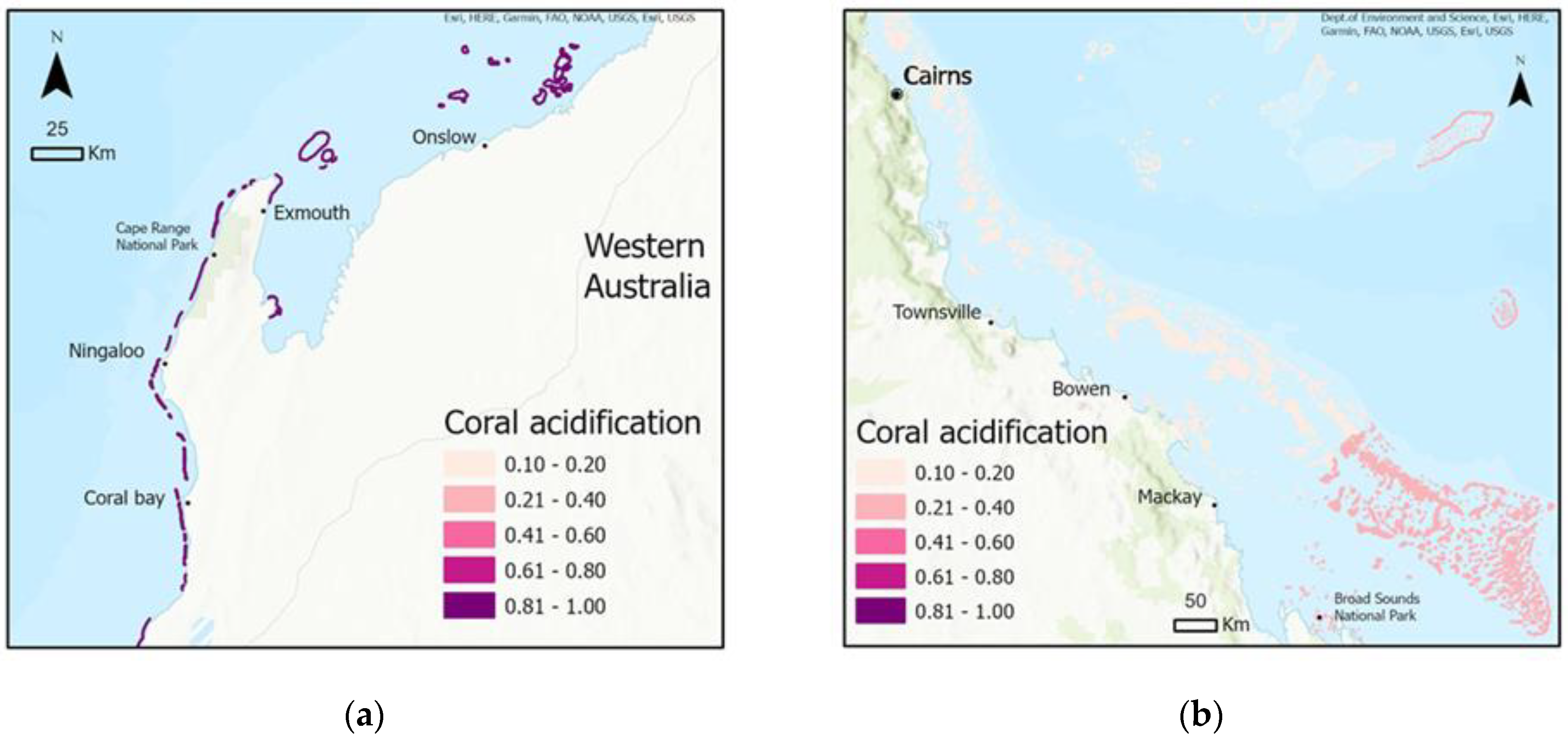
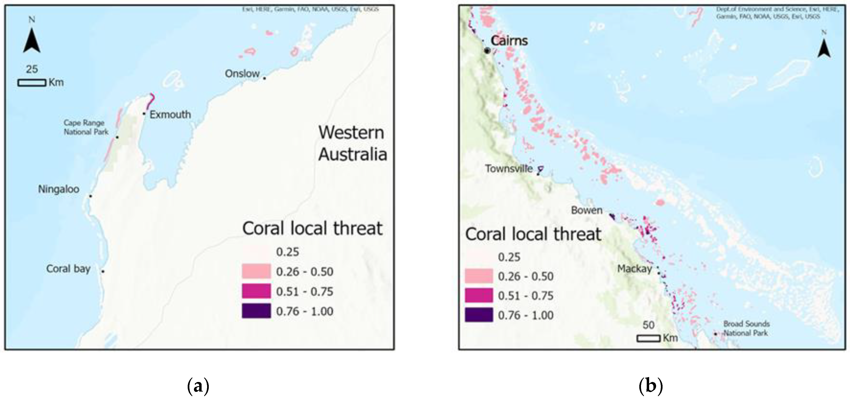
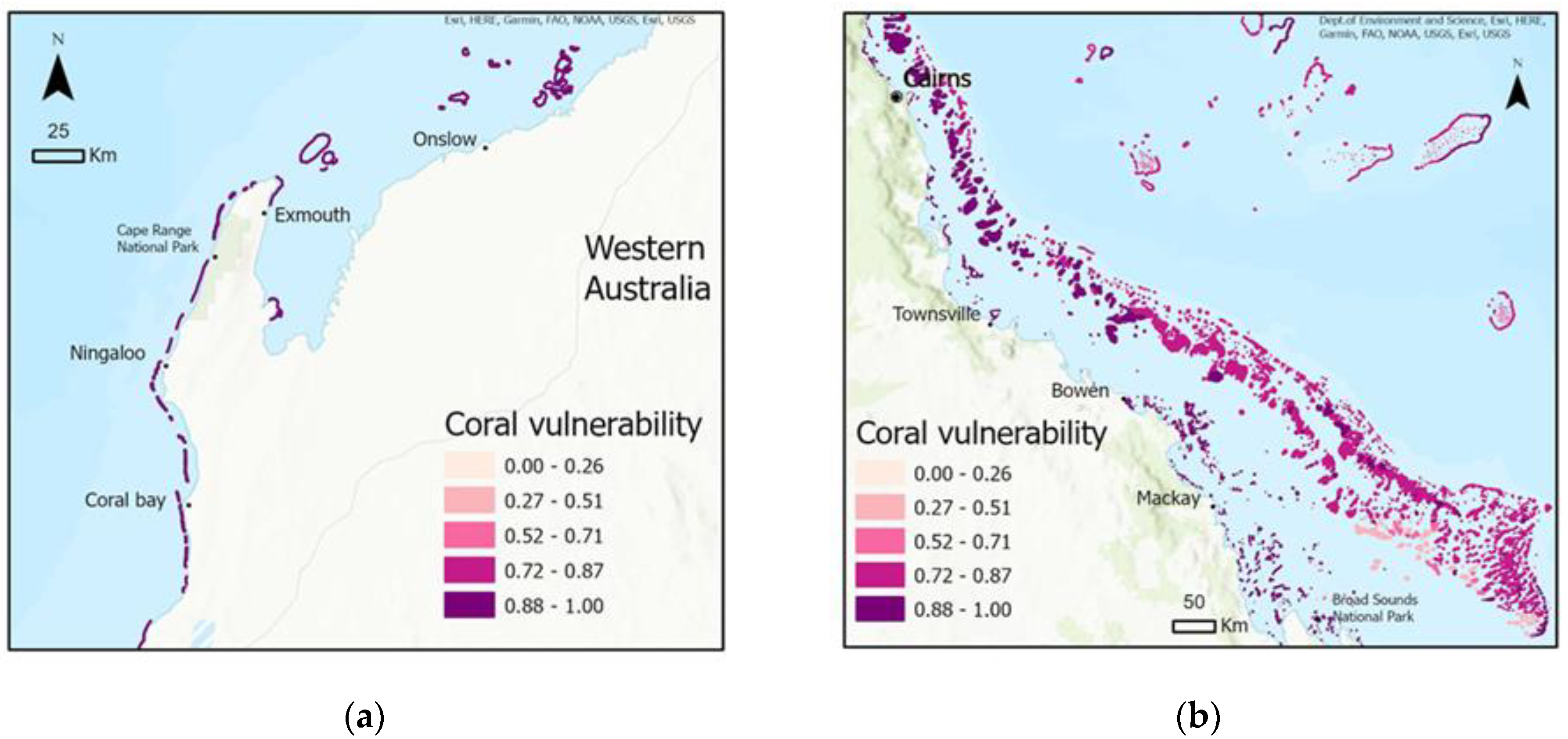
3.3. Vulnerability
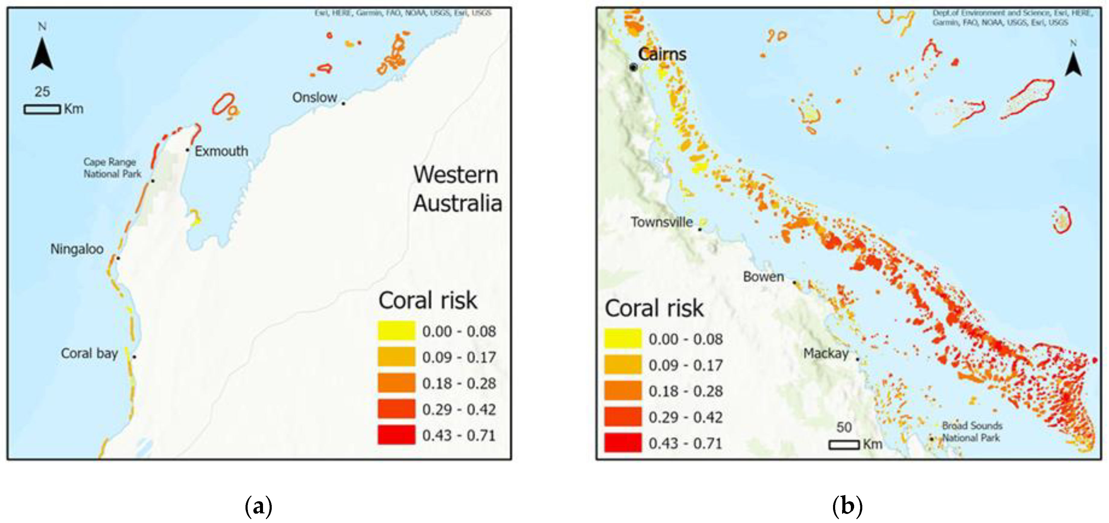
3.4. Tropical Cyclone Risk to Corals
3.5. Limitations
4. Conclusions
Author Contributions
Funding
Data Availability Statement
Acknowledgments
Conflicts of Interest
References
- Burston, J.M.; Taylor, D.; Dent, J.; Churchill, J. Australia-wide tropical cyclone multi-hazard risk assessment. In Australasian Coasts & Ports 2017: Working with Nature; Engineers Australia, PIANC Australia and Institute of Professional Engineers: Carins, Australia, 2017; pp. 185–191. [Google Scholar]
- Do, C.; Kuleshov, Y. Multi-hazard Tropical Cyclone Risk Assessment for Australia. Nat. Hazards Earth Syst. Sci. Discuss. 2022, 1–19. [Google Scholar] [CrossRef]
- IPCC. Climate Change 2022: Impacts, Adaptation, and Vulnerability. Contribution of Working Group II to the Sixth Assessment Report of the Intergovernmental Panel on Climate Change; Cambridge University Press: Cambridge, UK, 2022. [Google Scholar]
- Cheal, A.J.; MacNeil, M.A.; Emslie, M.J.; Sweatman, H. The threat to coral reefs from more intense cyclones under climate change. Global Chang. Biol. 2017, 23, 1511–1524. [Google Scholar] [CrossRef] [PubMed]
- Scoffin, T. The geological effects of hurricanes on coral reefs and the interpretation of storm deposits. Coral Reefs 1993, 12, 203–221. [Google Scholar] [CrossRef]
- Done, T. Effects of tropical cyclone waves on ecological and geomorphological structures on the Great Barrier Reef. Cont. Shelf Res. 1992, 12, 859–872. [Google Scholar] [CrossRef]
- Beeden, R.; Maynard, J.; Puotinen, M.; Marshall, P.; Dryden, J.; Goldberg, J.; Williams, G. Impacts and recovery from severe tropical cyclone Yasi on the Great Barrier Reef. PLoS ONE 2015, 10, e0121272. [Google Scholar] [CrossRef]
- Fabricius, K.E.; De’Ath, G.; Puotinen, M.L.; Done, T.; Cooper, T.F.; Burgess, S.C. Disturbance gradients on inshore and offshore coral reefs caused by a severe tropical cyclone. Limnol. Oceanogr. 2008, 53, 690–704. [Google Scholar] [CrossRef]
- Harmelin-Vivien, M.L. The effects of storms and cyclones on coral reefs: A review. J. Coast. Res. 1994, 12, 211–231. [Google Scholar]
- Burke, L.; Reytar, K.; Spalding, M.; Perry, A. Reefs at Risk Revisited; World Resources Institute: Washington, DC, USA, 2011; Available online: http://pdf.wri.org/reefs_at_risk_revisited.pdf (accessed on 26 October 2022).
- Munday, P.L.; Jones, G.P.; Pratchett, M.S.; Williams, A.J. Climate change and the future for coral reef fishes. Fish Fish. 2008, 9, 261–285. [Google Scholar] [CrossRef]
- Hoegh-Guldberg, O. Climate change, coral bleaching and the future of the world’s coral reefs. Mar. Freshw. Res. 1999, 50, 839–866. [Google Scholar] [CrossRef] [Green Version]
- Pachauri, R.K.; Allen, M.R.; Barros, V.R.; Broome, J.; Cramer, W.; Christ, R.; Church, J.A.; Clarke, L.; Dahe, Q.; Dasgupta, P.; et al. Climate Change 2014: Synthesis Report. Contribution of Working Groups I, II and III to the Fifth Assessment Report of the Intergovernmental Panel on Climate Change; Pachauri, R., Meyer, L., Eds.; IPCC: Geneva, Switzerland, 2014. [Google Scholar]
- Beck, M.W.; Losada, I.J.; Menendez, P.; Reguero, B.G.; Diaz-Simal, P.; Fernandez, F. The global flood protection savings provided by coral reefs. Nat. Commun. 2018, 9, 2186. [Google Scholar] [CrossRef] [Green Version]
- Mendelsohn, R.; Zheng, L. Coastal resilience against storm surge from tropical cyclones. Atmosphere 2020, 11, 725. [Google Scholar] [CrossRef]
- Moberg, F.; Folke, C. Ecological goods and services of coral reef ecosystems. Ecol. Econ. 1999, 29, 215–233. [Google Scholar] [CrossRef]
- Costanza, R.; De Groot, R.; Sutton, P.; Van der Ploeg, S.; Anderson, S.J.; Kubiszewski, I.; Farber, S.; Turner, R.K. Changes in the global value of ecosystem services. Glob. Environ. Chang. 2014, 26, 152–158. [Google Scholar] [CrossRef]
- Cinner, J. Coral reef livelihoods. Curr. Opin. Environ. Sustain. 2014, 7, 65–71. [Google Scholar] [CrossRef]
- Deloitte Access Economics. At What Price? The Economic, Social and Icon Value of the Great Barrier Reef; Deloitte: Brisbane, Australia, 2017. [Google Scholar]
- Reguero, B.G.; Storlazzi, C.D.; Gibbs, A.E.; Shope, J.B.; Cole, A.D.; Cumming, K.A.; Beck, M.W. The value of US coral reefs for flood risk reduction. Nat. Sustain. 2021, 4, 688–698. [Google Scholar] [CrossRef]
- McLachlan, E. Seagulls on the airstrip: Indigenous perspectives on cyclone vulnerability awareness and mitigation strategies for remote communities in the Gulf of Carpentaria. Aust. J. Emerg. Manag. 2003, 18, 4–12. [Google Scholar]
- Mangubhai, S. Impact of Tropical Cyclone Winston on Coral Reefs in the Vatu-i-Ra Seascape; Wildlife Conservation Society: Suva, Fuji, 2016. [Google Scholar]
- Puotinen, M.; Maynard, J.A.; Beeden, R.; Radford, B.; Williams, G.J. A robust operational model for predicting where tropical cyclone waves damage coral reefs. Sci. Rep. 2016, 6, 26009. [Google Scholar] [CrossRef] [Green Version]
- UNESCO. World Heritage Convention—Properties Incscribed on the World Heritage List. Available online: https://whc.unesco.org/en/statesparties/au (accessed on 21 October 2021).
- Crichton, D. The Risk Triangle. In Natural Disaster Management; Ingleton, J., Ed.; Tudor Rose: London, UK, 1999; pp. 102–103. [Google Scholar]
- Schneiderbauer, S.; Ehrlich, D. Risk, hazard and people’s vulnerability to natural hazards. A review of definitions, concepts and data. Eur. Comm. Jt. Res. Cent. EUR 2004, 21410, 40. [Google Scholar]
- Arthur, C. Tropical Cyclone Hazard Assessment 2018. Geosci. Aust. Rec. 2018/40 2018. [Google Scholar] [CrossRef]
- Tittensor, D.P.; Mora, C.; Jetz, W.; Lotze, H.K.; Ricard, D.; Berghe, E.V.; Worm, B. Global patterns and predictors of marine biodiversity across taxa. Nature 2010, 466, 1098–1101. [Google Scholar] [CrossRef]
- Dustan, P.; Doherty, O.; Pardede, S. Digital reef rugosity estimates coral reef habitat complexity. PLoS ONE 2013, 8, e57386. [Google Scholar] [CrossRef]
- Graham, N.A.; Nash, K.L. The importance of structural complexity in coral reef ecosystems. Coral Reefs 2013, 32, 315–326. [Google Scholar] [CrossRef]
- Graham, N.A.; Jennings, S.; MacNeil, M.A.; Mouillot, D.; Wilson, S.K. Predicting climate-driven regime shifts versus rebound potential in coral reefs. Nature 2015, 518, 94–97. [Google Scholar] [CrossRef] [PubMed]
- Jenness, J.S. Calculating landscape surface area from digital elevation models. Wildl. Soc. Bull. 2004, 32, 829–839. [Google Scholar] [CrossRef]
- Huang, Z.C.; Lenain, L.; Melville, W.K.; Middleton, J.H.; Reineman, B.; Statom, N.; McCabe, R.M. Dissipation of wave energy and turbulence in a shallow coral reef lagoon. J. Geophys. Res. Ocean. 2012, 117. [Google Scholar] [CrossRef]
- Knudby, A.; Jupiter, S.; Roelfsema, C.; Lyons, M.; Phinn, S. Mapping coral reef resilience indicators using field and remotely sensed data. Remote Sens. 2013, 5, 1311–1334. [Google Scholar] [CrossRef] [Green Version]
- Group, G.B.C. The GEBCO_2019 grid—A continuous terrain model of the global oceans and land. Br. Oceanogr. Data Cent. Natl. Oceanogr. Cent. NERC 2019. Available online: https://www.gebco.net/data_and_products/gridded_bathymetry_data/ (accessed on 1 September 2022).
- BoM; CSIRO. State of the Climate 2020; BoM, CSIRO: Canberra, Australia, 2020. [Google Scholar]
- Abraham, J.P.; Baringer, M.; Bindoff, N.L.; Boyer, T.; Cheng, L.; Church, J.A.; Conroy, J.L.; Domingues, C.M.; Fasullo, J.T.; Gilson, J. A review of global ocean temperature observations: Implications for ocean heat content estimates and climate change. Rev. Geophys. 2013, 51, 450–483. [Google Scholar] [CrossRef] [Green Version]
- Donner, S.D.; Skirving, W.J.; Little, C.M.; Oppenheimer, M.; Hoegh-Guldberg, O. Global assessment of coral bleaching and required rates of adaptation under climate change. Global Chang. Biol. 2005, 11, 2251–2265. [Google Scholar] [CrossRef]
- Hughes, T.P.; Anderson, K.D.; Connolly, S.R.; Heron, S.F.; Kerry, J.T.; Lough, J.M.; Baird, A.H.; Baum, J.K.; Berumen, M.L.; Bridge, T.C. Spatial and temporal patterns of mass bleaching of corals in the Anthropocene. Science 2018, 359, 80–83. [Google Scholar] [CrossRef] [Green Version]
- Rowan, R. Diversity and ecology of zooxanthellae on coral reefs. J. Phycol. 1998, 34, 407–417. [Google Scholar] [CrossRef]
- Douglas, A. Coral bleaching––how and why? Mar. Pollut. Bull. 2003, 46, 385–392. [Google Scholar] [CrossRef] [PubMed]
- Baker, A.C.; Glynn, P.W.; Riegl, B. Climate change and coral reef bleaching: An ecological assessment of long-term impacts, recovery trends and future outlook. Estuar. Coast. Shelf Sci. 2008, 80, 435–471. [Google Scholar]
- Berry, L.; Taylor, A.R.; Lucken, U.; Ryan, K.P.; Brownlee, C. Calcification and inorganic carbon acquisition in coccolithophores. Funct. Plant Biol. 2002, 29, 289–299. [Google Scholar] [CrossRef] [PubMed] [Green Version]
- UNEP-WCMC; WorldFish Centre; WRI; TNC. Global Distribution of Warm-Water Coral Reefs, Compiled from Multiple Sources Including the Millennium Coral Reef Mapping Project; UNEP World Conservation Monitoring Centre: Cambridge, UK, 2010. [Google Scholar]
- Choi, J.-W.; Cha, Y.; Kim, H.-D.; Kang, S.-D. Latitudinal change of tropical cyclone maximum intensity in the western North Pacific. Adv. Meteorol. 2016, 2016, 5829162. [Google Scholar] [CrossRef]
- AIMS. Coral Bleaching Events. Available online: https://www.aims.gov.au/research-topics/environmental-issues/coral-bleaching/coral-bleaching-events (accessed on 22 October 2021).
- Pearce, A.; Jackson, G.; Moore, J.; Feng, M.; Gaughan, D.J. The “Marine Heat Wave” Off Western Australia during the Summer of 2010/11; Government of Western Australia, Department of Fisheries: North Beach, Australia, 2011. [Google Scholar]
- Hughes, T.P.; Kerry, J.T.; Álvarez-Noriega, M.; Álvarez-Romero, J.G.; Anderson, K.D.; Baird, A.H.; Babcock, R.C.; Beger, M.; Bellwood, D.R.; Berkelmans, R. Global warming and recurrent mass bleaching of corals. Nature 2017, 543, 373–377. [Google Scholar] [CrossRef]
- Babcock, R.; Thomson, D.; Haywood, M.; Vanderklift, M.; Pillans, R.; Rochester, W.; Miller, M.; Speed, C.; Shedrawi, G.; Field, S. Recurrent coral bleaching in north-western Australia and associated declines in coral cover. Mar. Freshw. Res. 2020, 72, 620–632. [Google Scholar] [CrossRef]
- IUCN. Great Barrier Reef 2020 Conservation Outlook Assessment; IUCN: World Heritage Outlook: Gland, Switzerland, 2020. [Google Scholar]
- Foster, G.; Rahmstorf, S. Global temperature evolution 1979–2010. Environ. Res. Lett. 2011, 6, 044022. [Google Scholar] [CrossRef]
- Tyrrell, T. Calcium carbonate cycling in future oceans and its influence on future climates. J. Plankton Res. 2008, 30, 141–156. [Google Scholar] [CrossRef] [Green Version]
- Orr, J.C.; Fabry, V.J.; Aumont, O.; Bopp, L.; Doney, S.C.; Feely, R.A.; Gnanadesikan, A.; Gruber, N.; Ishida, A.; Joos, F. Anthropogenic ocean acidification over the twenty-first century and its impact on calcifying organisms. Nature 2005, 437, 681–686. [Google Scholar] [CrossRef] [Green Version]
- IUCN. Ningaloo Coast 2020 Conservation Outlook Assessment; IUCN: World Heritage Outlook: Gland, Switzerland, 2020. [Google Scholar]
- Lenton, A.; McInnes, K.L. Marine projections of warming and ocean acidification in the Australasian region. Aust. Meteorol. Oceanogr. J. 2015, 65, S1–S28. [Google Scholar] [CrossRef]
- Kobryn, H.T.; Wouters, K.; Beckley, L.E.; Heege, T. Ningaloo reef: Shallow marine habitats mapped using a hyperspectral sensor. PLoS ONE 2013, 8, e70105. [Google Scholar] [CrossRef] [PubMed]


| Indicator | Dataset Used | Source | Year |
|---|---|---|---|
| Hazard | |||
| Wind hazard | Raster Cyclone wind, 100yr return period | Geosciences Australia [27] | 2018 |
| Exposure | |||
| Biodiversity | Global patterns of marine biodiversity (species richness) across 13 major species groups | UNEP-WCMC [28] | 2010 |
| Rugosity | Calculated as Standard deviation of bathymetry within that coral region | GEBCO [35] | 2019 |
| Vulnerability | |||
| Depth | Sea floor depth from bathymetry data | GEBCO [35] | 2019 |
| Local Integrated Threat | Threats from a wide range of human activities | UNEP Reefs at risk [10] | 2011 |
| Thermal Stress | Past and Projected Thermal Stress on Coral Reefs | UNEP Reefs at risk [10] | 2011 |
| Ocean Acidification | Past and Projected Ocean Acidification on Coral Reefs | UNEP Reefs at risk [10] | 2011 |
| Shape layers | |||
| Global Coral Map | Shapefile containing the distribution of Coral reefs | UNEP-WCMC [44] | 2010 |
Publisher’s Note: MDPI stays neutral with regard to jurisdictional claims in published maps and institutional affiliations. |
© 2022 by the authors. Licensee MDPI, Basel, Switzerland. This article is an open access article distributed under the terms and conditions of the Creative Commons Attribution (CC BY) license (https://creativecommons.org/licenses/by/4.0/).
Share and Cite
Do, C.; Saunders, G.E.; Kuleshov, Y. Assessment of Tropical Cyclone Risk to Coral Reefs: Case Study for Australia. Remote Sens. 2022, 14, 6150. https://doi.org/10.3390/rs14236150
Do C, Saunders GE, Kuleshov Y. Assessment of Tropical Cyclone Risk to Coral Reefs: Case Study for Australia. Remote Sensing. 2022; 14(23):6150. https://doi.org/10.3390/rs14236150
Chicago/Turabian StyleDo, Cameron, Georgia Elizabeth Saunders, and Yuriy Kuleshov. 2022. "Assessment of Tropical Cyclone Risk to Coral Reefs: Case Study for Australia" Remote Sensing 14, no. 23: 6150. https://doi.org/10.3390/rs14236150