Article

A New Magnetic Target Localization Method Based on Two-Point Magnetic Gradient Tensor

Key Laboratory of Instrumentation Science & Dynamic Measurement, Ministry of Education, North University of China, Taiyuan 030051, China
*
Author to whom correspondence should be addressed.
Remote Sens. 2022, 14(23), 6088; https://doi.org/10.3390/rs14236088
Submission received: 18 October 2022 / Revised: 25 November 2022 / Accepted: 27 November 2022 / Published: 30 November 2022

Abstract

:
The existing magnetic target localization methods are greatly affected by the geomagnetic field and exist approximation errors. In this paper, a two-point magnetic gradient tensor localization model is established by using the spatial relation between the magnetic target and the observation points derived from magnetic gradient tensor and tensor invariants. Based on the model, the equations relating to the position vector of magnetic target are constructed. Solving the equations, a new magnetic target localization method using only a two-point magnetic gradient tensor and no approximation errors is achieved. To accurately evaluate the localization accuracy of the method, a circular trajectory that varies in all three directions is proposed. Simulation results show that the proposed method is almost error-free in the absence of noise. After adding noise, the maximum relative error percentage is reduced by 28.4% and 2.21% compared with the single-point method and the other two-point method, respectively. Furthermore, the proposed method is not affected by the variation in the distance between two observation points. At a detection distance of 20 m, the maximum localization error is 1.86 m. In addition, the experiments also verify that the new method can avoid the influence of the geomagnetic field and the variation in the distance, and achieve high localization accuracy. The average relative error percentage in the y-direction is as low as 3.78%.

Graphical Abstract

1. Introduction

The magnetic field generated by a ferromagnetic target affects the distribution of the surrounding geomagnetic field, resulting in magnetic anomalies. By measuring the magnetic anomaly signals and processing the data, the location information of the target can be obtained [1]. The magnetic anomaly detection (MAD) technology has been widely used in underwater target detection [2,3,4], unexploded ordnance (UXO) detection [5,6,7], mineral exploration [8,9], biomagnetic signal detection [10,11], and many other fields due to its high concealment, strong penetration, fast speed, and high precision. Magnetic gradient tensor detection, compared with magnetic field scalar and vector detection, exhibits certain advantages, such as being less affected by the magnetization direction of the target, immunity to the background field, and providing more abundant magnetic field information [12]. At present, it has become a popular research topic in the field of magnetic anomaly detection.
Applying the magnetic gradient tensor to magnetic target localization was first proposed by Wynn in the 1970s [13,14], showing the great potential of the magnetic gradient tensor in high-precision localization. Since then, various localization methods based on the magnetic gradient tensor have been studied in detail. The single-point magnetic gradient tensor localization method was the first to receive attention. Wilson et al. [15] used the eigenvalues and eigenvectors of the magnetic gradient tensor to achieve point-to-point localization of the magnetic target. However, inherent four-fold ambiguity is present in the obtained solutions, and some additional information, such as magnetic field vectors, needs to be added to eliminate the ‘ghost’ solutions. Taking the localization of the radio frequency identification (RFID) tag as the background, Nara et al. [16] proposed to achieve the inversion of the location of the magnetic target by measuring the magnetic gradient tensor and the magnetic field vector at a single point, and gave the closed-form localization formula. Due to its advantages of simplicity and ease of implementation, it has attracted extensive attention [17,18], and is referred to herein as Nara’s single-point tensor (NSPT) method. However, since the magnetic field vector generated by the magnetic target is difficult to separate from the geomagnetic field, this method is governed by the geomagnetic field. Weigert et al. [19,20] proposed a Scalar Triangulation and Ranging (STAR) method based on tensor contraction, which has high real-time performance and can effectively avoid the influence of the geomagnetic field. However, since the contours of tensor contraction are approximated as a sphere, when the shape is actually an ellipsoid, this method has an inherent approximation error called asphericity error [21]. To improve the localization accuracy, several single-point higher-order magnetic gradient tensor localization methods have been proposed [22,23,24]. However, since the high-order quantity is greatly affected by the measurement noise of the instrument, these methods have high requirements regarding the accuracy of the sensor. In addition, some typical optimization algorithms, such as the differential evolution algorithm [25] and neural network algorithm [26], are also used to solve the nonlinear inverse problem. However, due to their complexity and time consumption, they are infeasible in real-time localization applications, and reliable initial parameters are required.
The above methods show that the information contained in the magnetic gradient tensor of only one observation point is not sufficient for high-precision localization. Therefore, multi-point magnetic gradient tensor localization methods have appeared [27]. Based on the eigenvalues and eigenvectors method, Liu et al. [28] supplemented the magnetic gradient tensor of another point and designed a two-point tensor measurement array to realize magnetic target localization. However, the solving process is complex, and prior information is required to determine the scope of the solution. Most importantly, it has not been experimentally verified. Liu [29] constructed an objective function based on magnetic moment constraints to achieve magnetic target localization, and designed a two-point tensor measurement system composed of two cross-tensor structures arranged vertically. This method has the advantages of high environmental noise tolerance and low sensor accuracy requirements, but it used the PSO algorithm to identify the parameters, resulting in poor real-time performance. Furthermore, the optimization method and parameter selection have a great impact on the localization accuracy, so the reliability of the algorithm is low. Based on the NSPT method, Xu [30] proposed a linear localization method using a two-point magnetic gradient tensor, and gave an analytical solution, denoted as Xu’s two-point tensor (XTPT) method. The average relative error percentages of the XTPT method in the three magnetic field directions are smaller than those of the single-point magnetic gradient tensor localization method, with a maximum reduction of 18.66% in the magnetic field x-direction. However, there is an approximate calculation in the inversion process, the condition of which is that the relative position between the two observation points tends to be infinitesimal; thus, the distance between the two observation points will introduce approximation errors.
The tensor invariants derived from the magnetic gradient tensor do not vary with the change in the coordinate system and exhibit great potential in reducing approximation errors [31]. They have appeared in many inversion methods, including the aforementioned eigenvalues and eigenvectors method, and the STAR method [32]. Following several years of research, Beiki et al. provided a detailed introduction to tensor invariants in 2012 [33]. Based on the magnetic gradient tensor and its invariants, this paper establishes a spatial relation localization model and proposes a new two-point tensor (NTPT) localization method. Only the magnetic gradient tensor of two observation points needs to be measured and no approximation error exists in the inversion process, thus solving the problems of the traditional localization method, i.e., it cannot eliminate the influence of the geomagnetic field and easily introduces approximate errors. In addition, a new simulation model is established to analyze the localization accuracy of the method. Both simulation and experimental results show that the proposed NTPT method can effectively avoid the influence of the geomagnetic field and the distance between the two observation points, and further improves the localization accuracy.

2. Methods

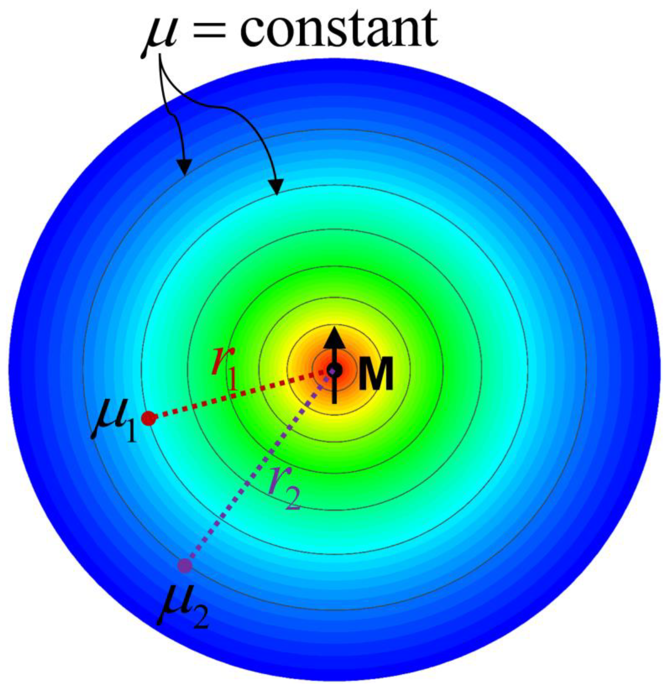
2.1. Magnetic Gradient Tensor and Tensor Invariants

The ferromagnetic target can be equivalent to a magnetic dipole when the detection distance between the target and the observation point is greater than 2.5 times the size of the target [34]. According to the Biot–Savart Law, the magnetic field vector B = ( B x , B y , B z ) generated by the magnetic dipole at any observation point can be expressed as:
B = μ 0 4 π 3 ( M · r ) r M r 2 r 5
where r = ( r x , r y . r z ) is the relative position vector from the magnetic dipole to the observation point, r = | r | . M = ( M x , M y , M z ) is the magnetic moment vector of the magnetic dipole, and μ 0 stands for the magnetic permeability of vacuum, μ 0 = 4 π × 10 7   T m / A .
The spatial rate of change of the three components of the magnetic field vector B in three mutually orthogonal directions is called the magnetic gradient tensor [22], denoted as G :
G = [ B x x B x y B x z B y x B y y B y z B z x B z y B z z ] = [ B x x B x y B x z B y x B y y B y z B z x B z y B z z ]
According to Maxwell’s equations, the divergence and curl of the magnetic field vector in the passive static magnetic field are both zero, that is, · B = 0 , × B = 0 , where is the mathematical symbol of the Hamiltonian. Combining the calculation rules of dot product and cross product, we can derive:
{ B x x + B y y + B z z = 0 B x y = B y x B x z = B z x B z y = B y z
Substituting Equation (3) into Equation (2), we can find that magnetic gradient tensor G is a symmetric real 3 × 3 matrix and traceless, there are three real eigenvalues, and the unit eigenvectors corresponding to different eigenvalues are mutually orthogonal. Clark [35] gave the expression of the three eigenvalues as follows:
{ λ m a x = 3 μ 0 m 8 π r 4 ( cos θ + 5 ( cos θ ) 2 + 4 ) λ m e d = 3 μ 0 m 4 π r 4 cos θ λ m i n = 3 μ 0 m 8 π r 4 ( cos θ 5 ( cos θ ) 2 + 4 )
where m = | M | is the magnitude of the magnetic moment vector of the magnetic dipole, θ is the angle between the relative position vector r and the magnetic moment vector M, and the three eigenvalues satisfy the relationship of λ m i n λ m e d λ m a x , | λ m e d | | λ m a x | , | λ m e d | | λ m i n | . Eigenvalues are scalar invariants of the magnetic gradient tensor, and any combination of eigenvalues is also scalar invariant [22]. In addition, the unit eigenvector corresponding to the eigenvalue with the smallest absolute value is perpendicular to both the magnetic moment vector and the relative position vector, which is called geometric invariant of the magnetic gradient tensor [33].
From (4) we can derive:
cos θ = λ m e d λ m e d 2 λ m a x λ m i n
Then, we define the normalized source strength (NSS), which is a combination of eigenvalues [35]:
μ = λ m e d 2 λ m a x λ m i n = 3 μ 0 m 4 π r 4
Evidently, the NSS is also a scalar invariant of the magnetic gradient tensor and has the advantage of being completely isotropic around the magnetic dipole.

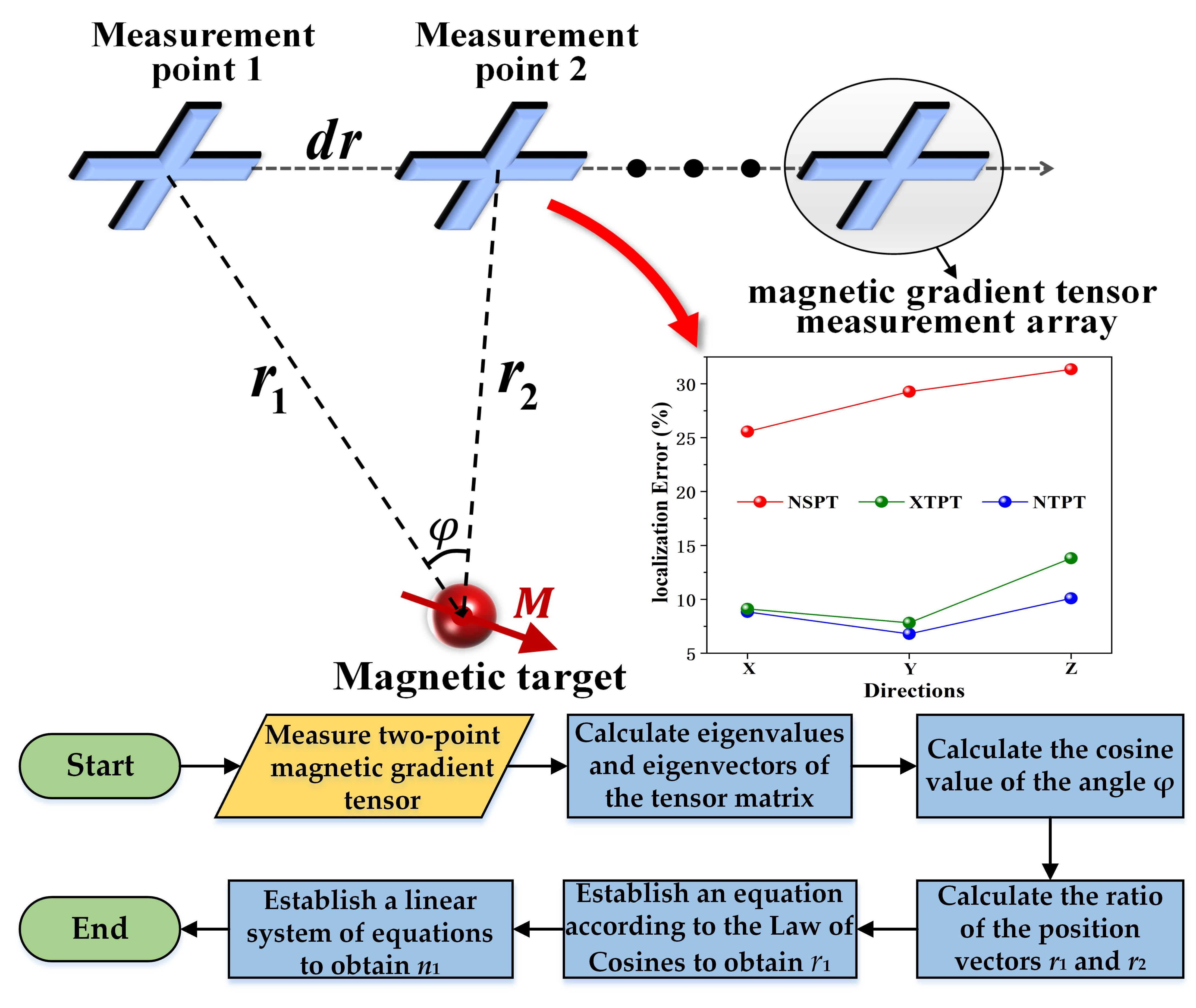
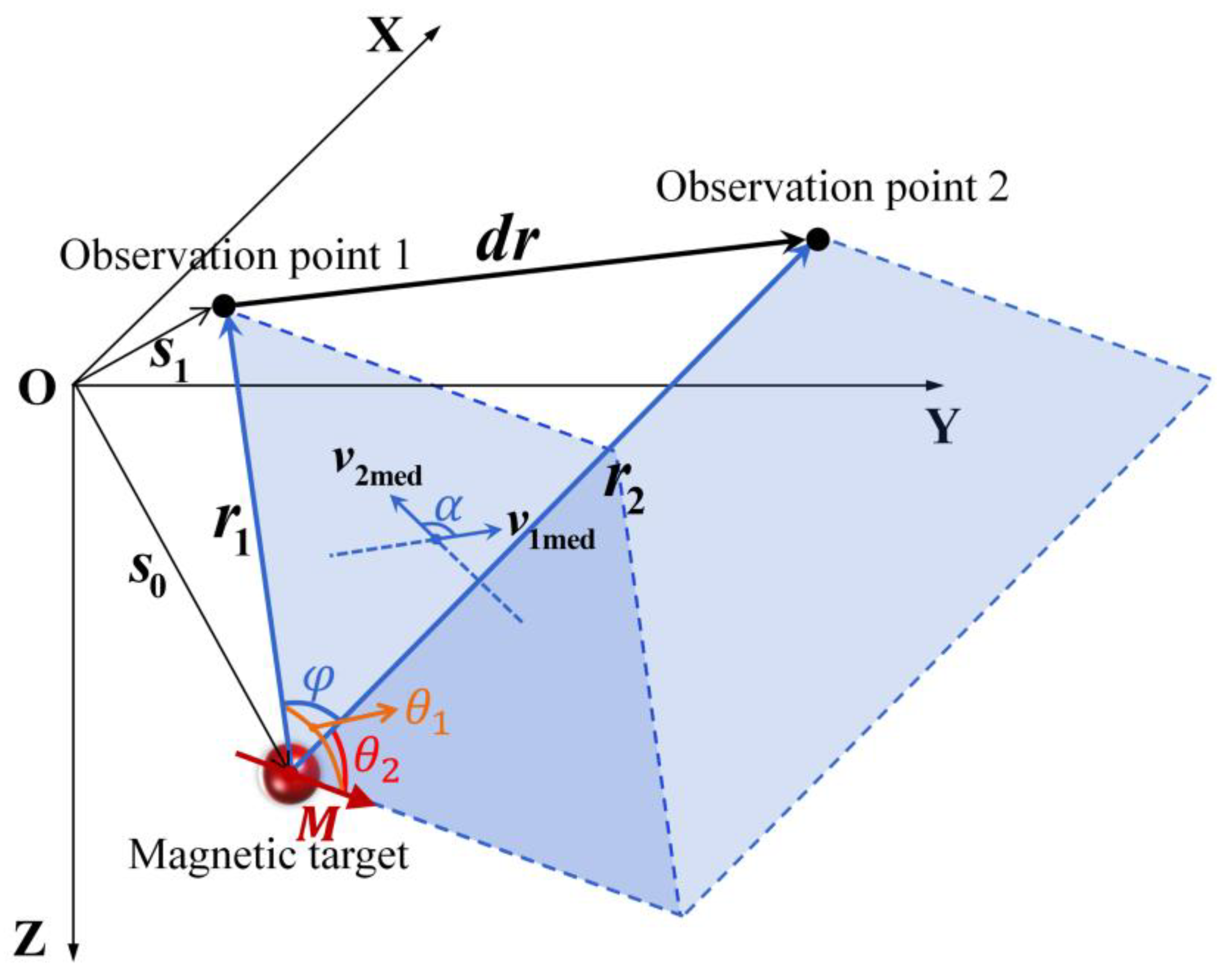
2.2. Localization Principle of the NTPT Method

The localization model of the NTPT method is shown in Figure 1. A Cartesian coordinate system is established with an arbitrary point in space as the origin, s 0 is the position vector of the magnetic target whose magnetic moment is M, r 1 is the relative position vector between the observation point 1 and the magnetic target, and r 2 is the relative position vector between the observation point 2 and the magnetic target. The offset vector d r from observation point 1 to observation point 2 can be described as:
d r = r 2 r 1
Suppose that v 1 med and v 2 med are the unit eigenvectors corresponding to the eigenvalues with the smallest absolute values of the magnetic gradient tensors at observation point 1 and 2, respectively. According to the tensor geometric invariant, we know that v 1 med is the normal vector of the plane defined by M and r 1 , and v 2 med is the normal vector of the plane defined by M and r 2 . The cosine value of the angle α between the two planes can be written as:
cos α = ± v 1 med · v 2 med
According to Equation (5), the cosine values of the angles θ 1 and θ 2 between the magnetic moment vector M of the magnetic target and the relative position vectors r 1 and r 2 can be obtained ( 0 θ 1 , θ 2 180 ° ). Then, the cosine value of the angle φ between r 1 and r 2 can be described by the following formula:
cos φ = cos θ 1 cos θ 2 + sin θ 1 sin θ 2 cos α
As shown in Figure 2, μ 1 and μ 2 are the NSS at observation points 1 and 2, respectively. Since the NSS information of the two observation points is generated by the same magnetic target, combined with the definition of NSS, it can be found that:
r 1 r 2 = ( μ 2 μ 1 ) 0.25 r 1 , r 2 > 0
where r 1 = | r 1 | , r 2 = | r 2 | are the magnitude of relative position vectors r 1 , r 2 , respectively. Then according to the Law of Cosines, we get:
( d r ) 2 = ( r 1 ) 2 + ( r 2 ) 2 2 r 1 r 2 cos φ
Substituting Equations (9) and (10) into Equation (11), r 1 can be easily obtained by solving the equation.
From the calculation formula of the included angle cosine of the vector, cos φ can also be expressed as:
cos φ = r 1 · r 2 r 1 r 2 = r 1 · ( r 1 + d r ) r 1 r 2 = r 1 2 + r 1 n 1 · d r r 1 r 2
where n 1 is the unit direction vector of relative position vectors r 1 . According to the tensor geometric invariant, r 1 · v 1 med = 0 , r 2 · v 2 med = 0 . Simplifying the equations, we can get:
n 1 · v 1 med = 0
( n 1 + d r r 1 ) · v 2 med = 0
Solving the linear system of equations consisting of Equations (12)–(14), the unit direction vector n 1 can be obtained. The position vector of magnetic target is given by:
s 0 = s 1 r 1
It is worth noting that the uncertainty of the sign in the Equation (8) will lead to non-unique localization results. The following method is used to determine the unique value of cos α : calculate the values of d r · v 1 med and d r · v 2 med , respectively; if the signs of the two calculation results are the same, then cos α = v 1 med · v 2 med , otherwise cos α = v 1 med · v 2 med .
In summary, the implementation steps of the NTPT method are: (1) Calculate the cosine value of the angle between the relative position vectors r 1 and r 2 according to the spatial relations derived from the magnetic gradient tensor and invariants. (2) Calculate the ratio of the magnitudes of the relative position vectors r 1 and r 2 . (3) Establish an equation according to the Law of Cosines, and solve to obtain r 1 . (4) Establish a linear system of equations related to n 1 according to the spatial relations, and solve to obtain n 1 . During the whole inversion process, only the magnetic gradient tensors of the two observation points and the offset vector between the two observation points are used. There is no need to measure the components of the magnetic field vector, so the proposed method is unaffected by the geomagnetic field. Moreover, iterative computations and approximate calculations are not used in the method, which greatly reduces the complexity of the method and does not introduce approximation errors.

3. Simulations

In order to evaluate the localization ability of the proposed method, several sets of simulation experiments were carried out. Any point in space is set as the origin, the coordinates of the magnetic target are (−19, −30, −23) m, and the magnetic moment is (389, 225, 779) A·m2. For the convenience of operation, the observation points in previous simulations usually move along the circular trajectory parallel to the x–y-plane, ignoring the influence of different z-coordinates, which may prevent the localization accuracy of the proposed method from being accurately estimated. As shown in Figure 3, we choose the circular trajectory with a 30° angle to the x–y plane, namely, the elevation of the normal vector of the plane where the trajectory is located is 60°, and the azimuth is 0°. The radius of the circular trajectory is 12 m. The magnitude of the relative position vector from the magnetic target to the center of the circular trajectory is 16 m and the direction is parallel to the normal vector of the trajectory. We define α as the rotation angle of the observation point, which represents the angle between the projection of the x-axis on the plane where the circular trajectory is located and the line connecting the observation point and the center of the circular trajectory. Observation points at different positions correspond to different rotation angles.

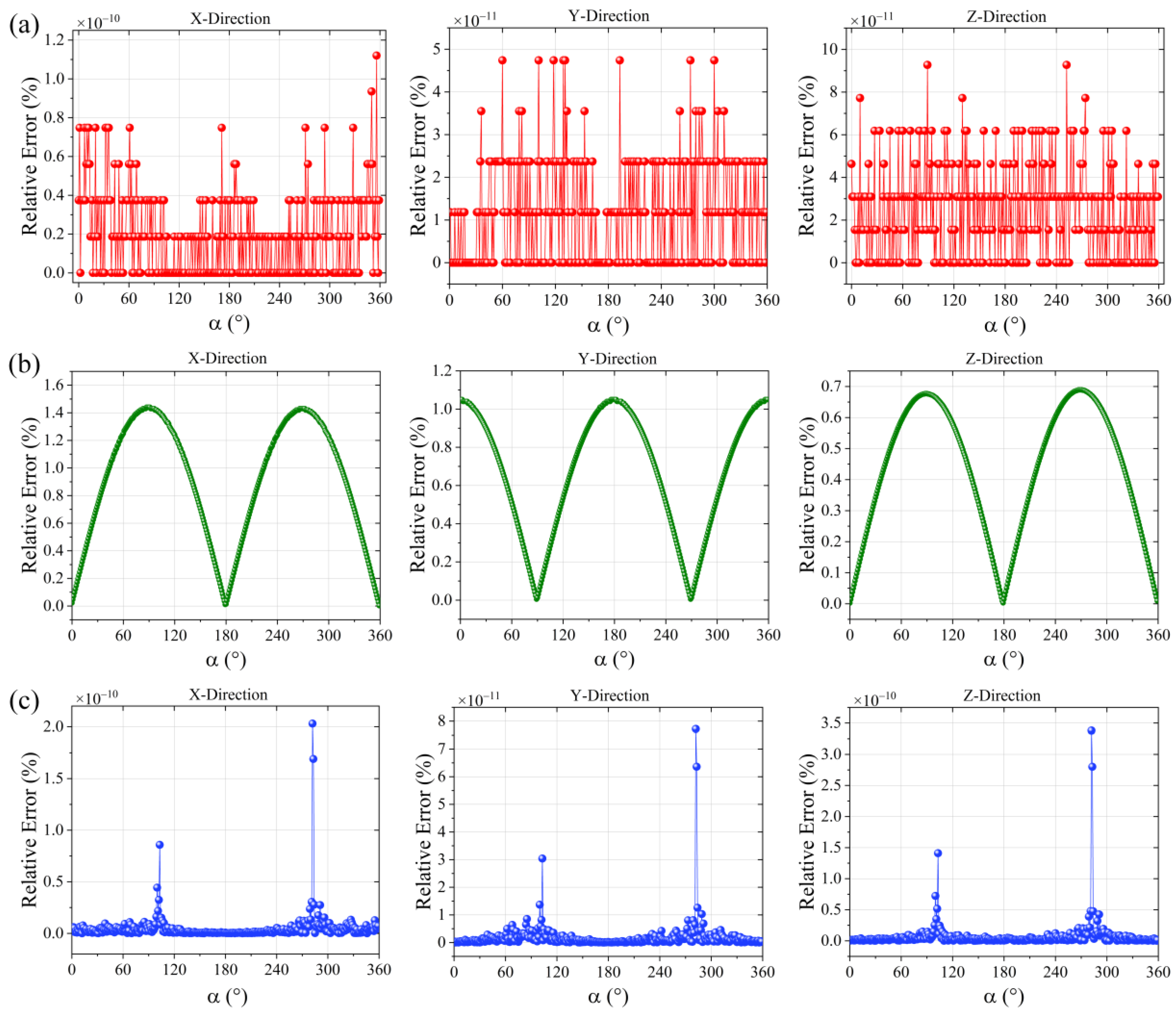
3.1. Without the Influence of the Noise

First, a simulation experiment without the influence of noise is carried out to verify the proposed method. Assuming that the observation points move at equal intervals along the circular trajectory, the rotation angle varies from 0 to 359°, and the interval is 1°. Any adjacent points form a group to complete the two-point localization. The NSPT, XTPT, and NTPT methods are used to conduct the simulation, and Figure 4 shows the relative error percentages of the three methods in the x-, y-, and z-directions.
It can be seen that all three localization methods can achieve good localization results in x-, y-, and z-directions in the case of without adding noise, and the relative error percentages of the XTPT method are slightly higher. The maximum error of the XTPT method is 1.44% in the x-direction, while the maximum error of the proposed NTPT method is 3.38 × 10⁻¹⁰% in the z-direction, which can be considered almost error-free. The minimum error of the NTPT method is 1.26 × 10⁻¹⁵% in the x-direction when the rotation angle is 191°, and the minimum errors of XTPT method and NSPT method are 2.45 × 10⁻³% and 1.18 × 10⁻¹⁴%, respectively. Therefore, simulation results indicate that the proposed method is theoretically feasible and almost error-free in all three directions without considering noise.

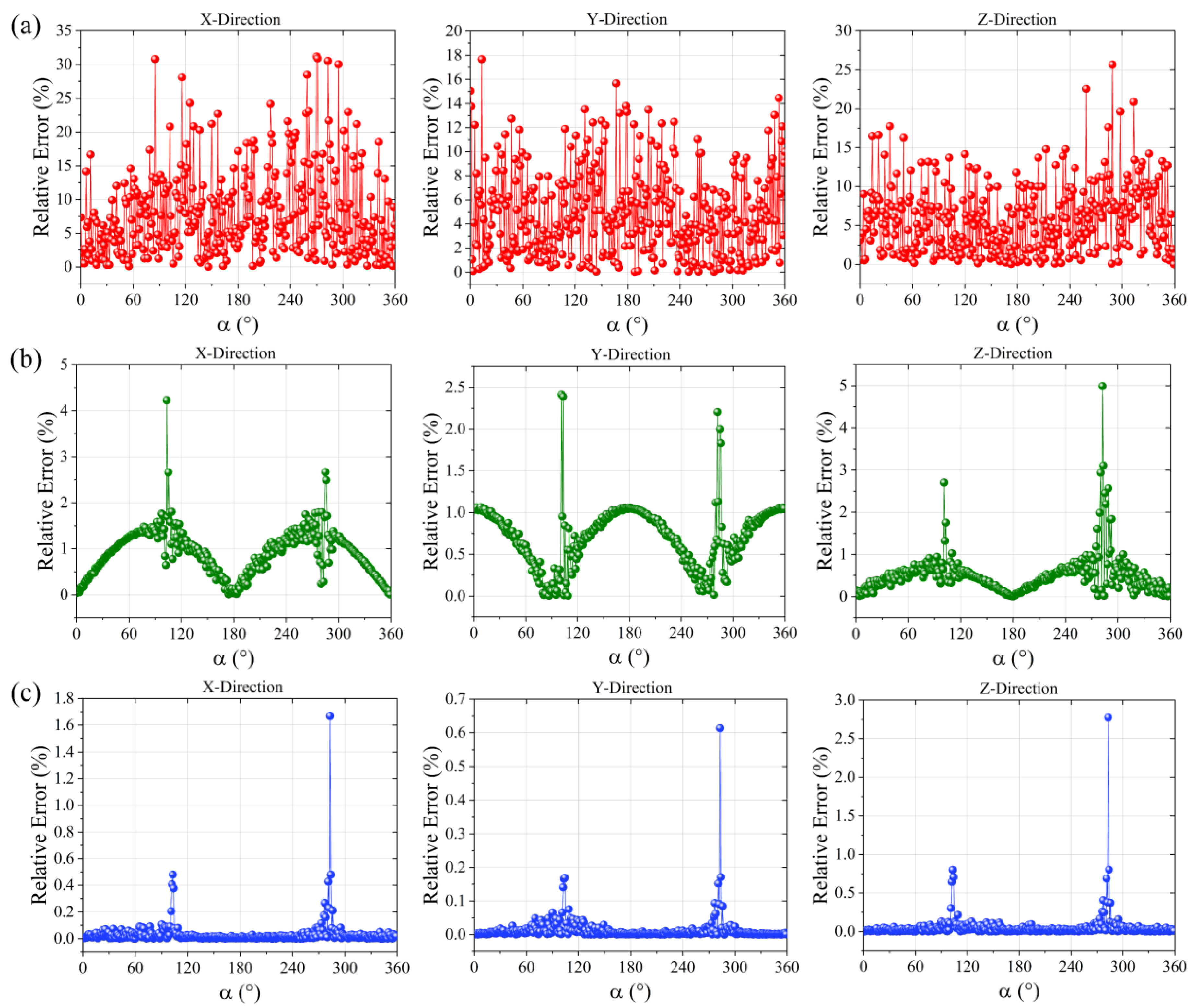
3.2. With the Influence of the Noise

In practical applications, the influence of noise is unavoidable, so it is necessary to carry out simulation experiments with added noise to verify the robustness of the method. Generally, the magnetic field generated by the magnetic target cannot exist alone, and will be superimposed with the geomagnetic field. Therefore, the noise includes instrument measurement noise and geomagnetic field measurement noise. White Gaussian noise with a mean value of zero and a standard deviation of 0.01 nT/m was added as the instrument measurement noise, and white Gaussian noise with a mean value of zero and a standard deviation of 1 nT was added as the geomagnetic field measurement noise. Other simulation conditions were consistent with those of the first simulation. The simulation results are shown in Figure 5.
Comparing Figure 4 and Figure 5, it is clear that no matter which method is used, the relative error percentages in the x-, y-, and z-directions increase after adding noise. However, the growth rate of the single-point method is significantly higher than that of the two-point method. The maximum error of the NSPT method is 31.18% when the rotation angle of the observation point is 270° in the x-direction, which is 31.18% higher than that without adding noise. By comparison, the maximum error of the NTPT and the XTPT are 2.78% and 4.99%, respectively, which are increased by 2.78% and 3.55%, respectively, compared with no noise. In addition, the maximum error of NTPT method is 28.4% and 2.21% lower than that of the NSPT method and XTPT method, respectively. The average relative error percentages of the three methods are shown in Table 1. The smaller the relative error percentage, the higher the localization accuracy. Obviously, regardless of the direction, the localization accuracy of the NTPT method is higher than that of the NSPT and XTPT methods. Therefore, the proposed NTPT method has the strongest anti-noise ability and highest localization accuracy, whereas the NSPT method is most affected by noise and has the lowest localization accuracy in each direction; this can be explained by the fact that the single-point method needs to measure three components of the magnetic field vector.

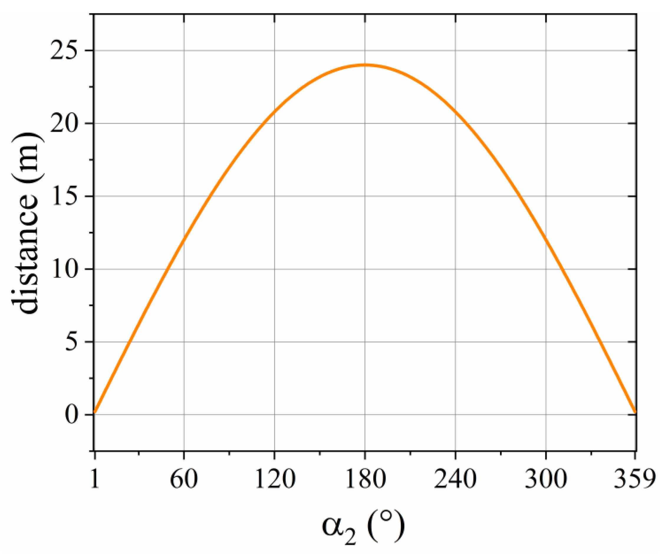
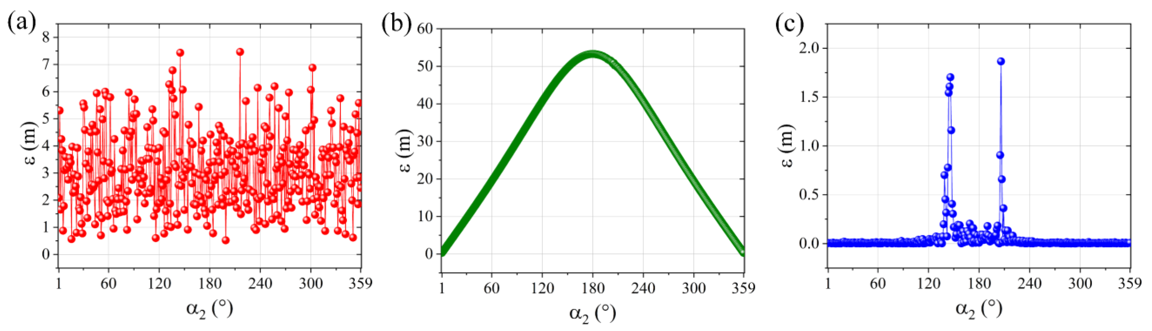
3.3. Influence of Distance between Observation Points

Since the distance between two observation points is arbitrary and unconstrained, it is necessary to analyze the influence of different distances on the localization results. Suppose that observation point 1 is located at the position of rotation angle α 1 = 0 ° and remains unchanged, and observation point 2 moves along circular trajectory and the rotation angle α 2 varies from 1° to 359° with an interval of 1°. Other simulation conditions are the same as those of the last simulation.
Figure 6 shows that, with the increase in the rotation angle of observation point 2, the distance between the two observation points increases first and then decreases, and reaches the maximum value when α 2 = 180 ° . The localization error ε is used as the evaluation index of the localization result:
ε = ( x x 0 ) 2 + ( y y 0 ) 2 + ( z z 0 ) 2
where x 0 , y 0 , z 0 are the real values of the position of the magnetic target, and x, y, z are the estimated values of the localization method. Figure 7 shows the variation in the localization error ε of the three methods with the increase in the rotation angle α 2 of the observation point 2.
Combining Figure 6 and Figure 7, it can be seen that, as the distance between the two observation points increases/decreases, the localization error of the XTPT increases/decreases. When the rotation angle α 2 is 180°, the distance between the two observation points reaches a maximum value of 24 m and, at the same time, the localization error of the XTPT reaches a maximum value of 53.29 m. However, the localization error of the proposed NTPT method, which is also a two-point tensor method, does not increase or decrease regularly with the increase/decrease in the distance; that is, the NTPT method is independent of the distance between the two observation points. The maximum error of the NTPT method is 1.86 m, and that of the NSPT method is up to 7.46 m. Furthermore, the minimum error of the NTPT method is 0.00024 m, whereas that of the NSPT and XTPT methods is 0.52 and 0.32 m, respectively. The simulation results indicates that the NTPT method is not only unaffected by the variation in the distance between the two observation points, but also has the highest localization accuracy, whereas the XTPT method is easily affected by the distance between the two observation points, which is due to the approximate calculation used in the inversion process. The condition for the approximate calculation is that the distance between the two observation points is as small as possible. Therefore, in order to achieve high localization accuracy, the XTPT method needs to constrain the distance between the two observation points.

4. Experiments and Result Analysis

4.1. Magnetic Gradient Tensor Measurement Array Model

According to relevant theory, there are only five independent components among all the magnetic gradient tensor components. As long as the five independent components are known, the magnetic gradient tensor can be obtained. Studies shows that the planar magnetic gradient tensor measurement array is easy to implement, and the center point of the structure is easy to determine [36]. A planar cross-shaped magnetic gradient tensor measurement array composed of four three-axis magnetometers is used in this paper, and the model is shown in Figure 8. The magnetometers are arranged symmetrically in pairs, and the baseline distances are both d. Based on the principle of difference on the same axis, the tensor matrix expression at the center point O of the cross-shaped structure can be written as:
G = 1 d [ B 1 x B 3 x B 2 x B 4 x B 1 y B 3 y B 2 y B 4 y B 1 z B 3 z B 2 z B 4 z ]

4.2. Experimental Verification and Result Analysis

In order to verify the actual effect of the proposed method, a field experiment was carried out in a space with a relatively stable magnetic field. As shown in Figure 9a, the magnetic gradient tensor measurement system includes a cross-shaped bracket, a planar cross-shaped magnetic gradient tensor measurement array, a power supply, and an acquisition module. The planar cross-shaped magnetic gradient tensor measurement array consists of four three-axis fluxgate magnetometers produced by British company Bartington, with a baseline distance of 40 cm. The error of the magnetic gradient full tensor obtained by the planar cross-shaped measurement array is due mainly to three aspects: using a finite difference to approximate the true first-order gradient, the noise of the magnetometers, and the residual error after measurement array calibration. The cross-shaped bracket is made of non-magnetic acrylic board. To ensure the consistency of acquisition accuracy, all sensor output signals are acquired by the same acquisition module. Furthermore, to reduce the influence of the diurnal variation of the geomagnetic field, the experiment was carried out at 0–3 A.M., and the ambient temperature was 20 °C. To avoid the influence of the ambient magnetic gradient, we measure the background gradient before placing the magnetic target. After placing the magnetic target, the background magnetic gradient is subtracted from the measured value of the magnetic sensor to obtain the final magnetic gradient data.
Due to the complexity of the construction of the circular trajectory platform, we chose the straight trajectory for the experiment. The experiment process is shown in Figure 9b. Taking the center point of the straight trajectory as the coordinate origin, the magnetic target was located at (−81.7, −49.6, 90.9) cm. The planar cross-shaped magnetic gradient tensor measurement array moved along the straight-line z = x, the total length of the trajectory was 180 cm, and the interval of measurement points was set to 30 cm. Therefore, seven sets of measurement data were obtained. The three-axis fluxgate magnetometer located at the center of the cross-shaped bracket was used to measure the three components of the magnetic field vector used in the NSPT method.

4.2.1. Localization with Adjacent Measurement Points

First, any adjacent measurement points are used for two-point tensor localization, that is, the distance between the two observation points is fixed at 30 cm. There are six sets of two-point localization solutions and seven sets of single-point localization solutions; Table 2 shows the relative error percentages of the NTPT, XTPT, and NSPT methods in three directions.
From Table 2, we can first find that the localization accuracy of the two-point tensor method is better than that of the single-point tensor method. The minimum errors of the NTPT method and XTPT method are 0.15% and 0.13%, respectively, whereas that of the NSPT method is up to 14.78%. Moreover, the maximum errors of the NTPT method and XTPT method in the x-direction are 13.01% and 14.59%, respectively, which are smaller than the minimum error of the NSPT method in the x-direction. The maximum error of the NSPT method is 44.31%, which is 28.18% and 26.78% higher than that of the NTPT method and the XTPT method, respectively. Furthermore, the average relative error percentages of the NTPT method and XTPT method in the three directions are all smaller than the average relative error percentages of the NSPT method, and the maximum average relative error percentage differences are 21.26% and 17.53% in the z-direction, respectively. Then, comparing the two two-point tensor methods, it can be found that the localization accuracy of the NTPT method is slightly higher than that of the XTPT method. The maximum error of NTPT method is 16.13% in the z-direction, whereas that of the XTPT method is 17.53% in the y-direction. The average relative error percentages in the x-, y-, and z-directions of the NTPT method are reduced by 0.28%, 1.02%, and 3.73%, respectively, compared with the XTPT method. The above conclusions are consistent with the simulation results in Section 3.2, which proves the correctness of the simulation experiments.

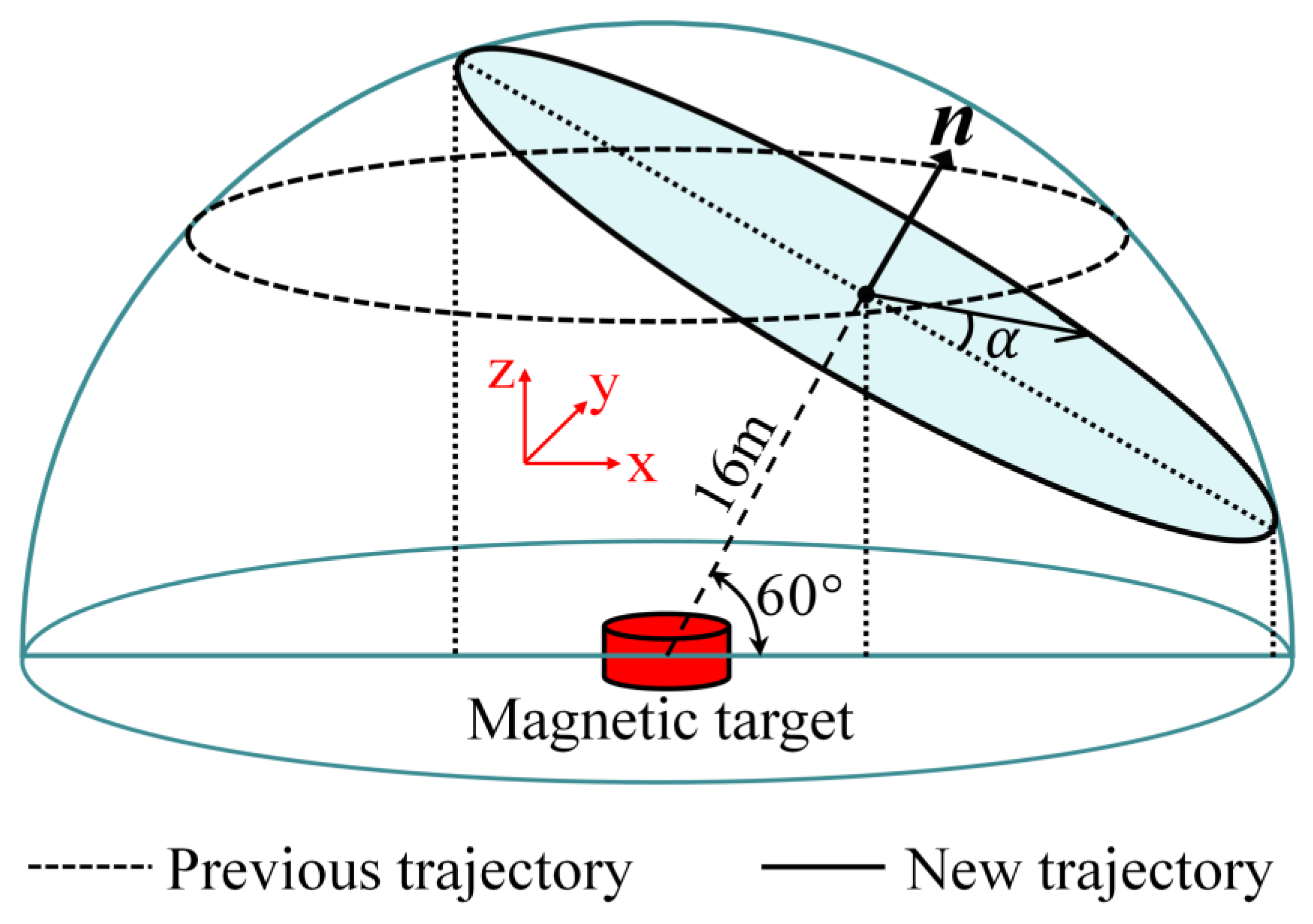
4.2.2. Localization with Variational Observation Point Distances

In order to verify the influence of the distance between the two observation points on the localization results of the two-point tensor method, the measurement data were reprocessed. We took the first measurement point as observation point 1 and kept this unchanged, and the remaining measurement points were sequentially regarded as observation point 2 to perform two-point localization. With the change in observation point 2, the distance between the two observation points gradually increased. A total of six sets of two-point localization solutions were obtained, and the relative error percentages are shown in Table 3.
Compared with the previous two-point localization using adjacent points, the relative error percentages of the XTPT method increase significantly in all three directions. The relative error percentages in the y- and z-directions increase exponentially with the distance between the two observation points, and the average relative error percentages increase by 40.71% and 48.29%, respectively. The average relative error percentage in the x-direction increases by 4%. Furthermore, when the distance between the two observation points is greater than 90 cm, the relative error percentages in the z-direction are greater than 53.99%, and the localization method can be considered invalid. However, the NTPT method is not affected by the distance between the two observation points. The relative error percentages of each point only fluctuate slightly due to the influence of random noise. The average relative error percentages in the z-direction increase by 0.95%, whereas those in the x- and y-directions decrease by 0.19% and 3.02%, respectively. Furthermore, the average relative error percentages of the NTPT method in all three directions are much smaller than those of the XTPT method.

5. Conclusions

The current localization methods based on the magnetic gradient tensor are susceptible to geomagnetic noise interference, can easily introduce approximation errors, and have a complex inversion process. To address these shortcomings, the NTPT method is proposed. This method realizes target localization according to the spatial relations between the magnetic target and the observation points. Considering the convenience of operation, previous simulations usually use latitude trajectories parallel to the x–y-plane to analyze the localization accuracy. In fact, slight changes in the z-coordinate can also affect the analysis of the localization results. Therefore, a special circular trajectory that changes in all three directions is used for simulation. Simulation results indicate that the proposed method has strong anti-noise ability. When noise is not considered, the method can achieve error-free localization. After adding noise, the maximum error is increased by 2.76%, whereas that of the XTPM and NSPT methods is increased by 3.55% and 30.89%, respectively. In addition, the NTPT method is not sensitive to the variation in the distance between the two points and has the highest localization accuracy. At a detection distance of 20 m, regardless of the change in the distance between two observation points, the maximum localization error is 1.86 m. The experimental results also prove that the NTPT method can avoid the interference of the geomagnetic field and the influence of the distance change between the observation points, and achieve high positioning accuracy. The maximum average error is reduced by 3.73% and 21.26% compared with the XTPT and NSPT methods, respectively.
If there are multiple measurement points, two measurement points at any position can be combined to achieve localization using the NTPT method, and multiple inversion solutions can be obtained with a small number of measurement points, so that the information of each measurement point can be fully utilized. The NTPT method has the potential for industrial, civil, and military applications, and indicates the direction for target detection based on magnetic gradient tensor. However, only prototype verification of the detection of a single target with a constant magnetic moment is performed in this paper. For the detection of multiple targets or targets with variable magnetic moments, further research is required. In addition, the errors introduced when calculating the magnitude of the relative position vector may be transmitted into the calculation of the unit direction vector, resulting in a considerable positioning error at some points. Therefore, there is still room for improvement. In the future, we will work on simultaneously solving the magnitude and unit direction vector of the relative position vector, and carry out feasibility analysis for practical application scenarios, such as unexploded ordnance detection, underwater target detection, vehicle detection, and mineral exploration.

Author Contributions

Conceptualization, G.L. and Y.Z.; Data curation, G.L., Y.Z. and C.W.; Formal analysis, G.L. and C.W.; Funding acquisition, Y.Z. and W.L.; Investigation, G.L. and Y.Z.; Methodology, G.L.; Project administration, G.L. and W.L.; Resources, Y.Z. and W.L.; Software, G.L. and Q.L.; Supervision, Y.Z., F.L. and W.L.; Validation, G.L., C.W. and Q.L.; Visualization, F.L.; Writing—original draft, G.L.; Writing—review and editing, G.L., Y.Z. and W.L. All authors have sufficiently participated in the study and provided useful advice. All authors have read and agreed to the published version of the manuscript.

Funding

This research was supported by the Innovative Research Group Project of the National Science Foundation of China, China (51821003), the National Science Foundation of Shanxi Province, China (201701D121065) and Fundamental Research Program of Shanxi Province (20210302124329).

Data Availability Statement

Not applicable.

Conflicts of Interest

The authors declare no conflict of interest.

References

  1. Jin, H.; Guo, J.; Wang, H.; Zhuang, Z.; Qin, J.; Wang, T. Magnetic Anomaly Detection and Localization Using Orthogonal Basis of Magnetic Tensor Contraction. IEEE Trans. Geosci. Remote Sens. 2020, 58, 5944–5954. [Google Scholar] [CrossRef]
  2. Lin, P.; Zhang, N.; Chang, M.; Xu, L. Research on the Model and the Location Method of Ship Shaft-Rate Magnetic Field Based on Rotating Magnetic Dipole. IEEE Access 2020, 8, 162999–163005. [Google Scholar] [CrossRef]
  3. Hu, S.; Tang, J.; Ren, Z.; Chen, C.; Zhou, C.; Xiao, X.; Zhao, T. Multiple Underwater Objects Localization With Magnetic Gradiometry. IEEE Geosci. Remote Sens. Lett. 2019, 16, 296–300. [Google Scholar] [CrossRef]
  4. Huang, Y.; Wu, L.H.; Sun, F. Underwater Continuous Localization Based on Magnetic Dipole Target Using Magnetic Gradient Tensor and Draft Depth. IEEE Geosci. Remote Sens. Lett. 2014, 11, 178–180. [Google Scholar] [CrossRef]
  5. Wiegert, R.; Oeschger, J. Generalized magnetic gradient contraction based method for detection, localization and discrimination of underwater mines and unexploded ordnance. In Proceedings of the OCEANS 2005 MTS/IEEE, Washington, DC, USA, 17–23 September 2005; pp. 1325–1332. [Google Scholar] [CrossRef]
  6. Chen, S.; Zhang, S.; Zhu, J.; Luan, X. Accurate Measurement of Characteristic Response for Unexploded Ordnance With Transient Electromagnetic System. IEEE Trans. Instrum. Meas. 2020, 69, 1728–1736. [Google Scholar] [CrossRef]
  7. Wang, L.; Zhang, S.; Chen, S.; Luo, C. Underground Target Localization Based on Improved Magnetic Gradient Tensor With Towed Transient Electromagnetic Sensor Array. IEEE Access 2022, 10, 25025–25033. [Google Scholar] [CrossRef]
  8. Schmidt, P.; Clark, D.; Leslie, K.; Bick, M.; Tilbrook, D.; Foley, C. GETMAG–a SQUID Magnetic Tensor Gradiometer for Mineral and Oil Exploration. Explor. Geophys. 2004, 35, 297–305. [Google Scholar] [CrossRef]
  9. Ma, G.; Zhao, Y.; Xu, B.; Li, L.; Wang, T. High-Precision Joint Magnetization Vector Inversion Method of Airborne Magnetic and Gradient Data with Structure and Data Double Constraints. Remote Sens. 2022, 14, 2508. [Google Scholar] [CrossRef]
  10. Her, A.Y.; Park, J.W. Repolarization Heterogeneity of Magnetocardiography Predicts Long-Term Prognosis in Patients with Acute Myocardial Infarction. Yonsei Med. J. 2016, 57, 1305–1306. [Google Scholar] [CrossRef]
  11. Primin, M.A.; Nedayvoda, I.V. Non-Contact Analysis of Magnetic Fields of Biological Objects: Algorithms for Data Recording and Processing. Cybern. Syst. Anal. 2020, 56, 848–862. [Google Scholar] [CrossRef]
  12. Schmidt, P.W.; Clark, D.A. The magnetic gradient tensor: Its properties and uses in source characterization. Lead. Edge 2006, 25, 75–78. [Google Scholar] [CrossRef] [Green Version]
  13. Wynn, W. Dipole tracking with a gradiometer. Nav. Ship Res. Dev. Lab. Informal Rep. NSRDL/PC 1972, 3493. [Google Scholar]
  14. Wynn, W.; Frahm, C.; Carroll, P.; Clark, R.; Wellhoner, J.; Wynn, M. Advanced superconducting gradiometer/magnetometer arrays and a novel signal processing technique. IEEE Trans. Magn. 1975, 11, 701–707. [Google Scholar] [CrossRef]
  15. Wilson, H. Analysis of the magnetic gradient tensor. Tech. Memo. 1985, 8, 5–13. [Google Scholar]
  16. Nara, T.; Suzuki, S.; Ando, S. A Closed-Form Formula for Magnetic Dipole Localization by Measurement of Its Magnetic Field and Spatial Gradients. IEEE Trans. Magn. 2006, 42, 3291–3293. [Google Scholar] [CrossRef]
  17. Yin, G.; Zhang, L.; Jiang, H.; Wei, Z.; Xie, Y. A closed-form formula for magnetic dipole localization by measurement of its magnetic field vector and magnetic gradient tensor. J. Magn. Magn. Mater. 2020, 499, 166274. [Google Scholar] [CrossRef]
  18. Higuchi, Y.; Nara, T.; Ando, S.; Kojima, F.; Kobayashi, F.; Nakamoto, H. A Truncated Singular Value Decomposition approach for locating a magnetic dipole with Euler’s equation. Int. J. Appl. Electromagn. Mech. 2016, 52, 67–72. [Google Scholar] [CrossRef]
  19. Wiegert, R.; Lee, K.; Oeschger, J. Improved magnetic STAR methods for real-time, point-by-point localization of unexploded ordnance and buried mines. In Proceedings of the OCEANS 2008, Quebec City, QC, Canada, 15–18 September 2008; pp. 1–7. [Google Scholar] [CrossRef] [Green Version]
  20. Wiegert, R.F. Magnetic STAR technology for real-time localization and classification of unexploded ordnance and buried mines. In Proceedings of the Detection and Sensing of Mines, Explosive Objects, and Obscured Targets XIV, Orlando, FL, USA, 13–17 April 2009; pp. 514–522. [Google Scholar] [CrossRef]
  21. Yin, G.; Li, P.; Wei, Z.; Liu, G.; Yang, Z.; Zhao, L. Magnetic dipole localization and magnetic moment estimation method based on normalized source strength. J. Magn. Magn. Mater. 2020, 502, 166450. [Google Scholar] [CrossRef]
  22. Yin, G.; Zhang, Y.; Fan, H.; Li, Z. Magnetic dipole localization based on magnetic gradient tensor data at a single point. J. Appl. Remote Sens. 2014, 8, 083596. [Google Scholar] [CrossRef]
  23. Sui, Y.; Leslie, K.; Clark, D. Multiple-Order Magnetic Gradient Tensors for Localization of a Magnetic Dipole. IEEE Magn. Lett. 2017, 8, 6506605. [Google Scholar] [CrossRef]
  24. Wang, B.; Ren, G.; Li, Z.; Li, Q. A third-order magnetic gradient tensor optimization algorithm based on the second-order improved central difference method. AIP Adv. 2021, 11, 065302. [Google Scholar] [CrossRef]
  25. Ding, X.; Li, Y.; Luo, M.; Chen, J.; Li, Z.; Liu, H. Estimating Locations and Moments of Multiple Dipole-Like Magnetic Sources From Magnetic Gradient Tensor Data Using Differential Evolution. IEEE Trans. Geosci. Remote Sens. 2022, 60, 1–13. [Google Scholar] [CrossRef]
  26. Tobely, T.E.; Salem, A. Position detection of unexploded ordnance from airborne magnetic anomaly data using 3-D self organized feature map. In Proceedings of the Fifth IEEE International Symposium on Signal Processing and Information Technology, Athens, Greece, 18–21 December 2005; pp. 322–327. [Google Scholar]
  27. Lin, P.; Zhang, N.; Lin, C.; Chang, M.; Xu, L. Two-point magnetic field positioning algorithm based on rotating magnetic dipole. Measurement 2021, 174, 109059. [Google Scholar] [CrossRef]
  28. Liu, J.H.; Li, X.H.; Zeng, X.N. Online magnetic target location method based on the magnetic gradient tensor of two points. Chin. J. Geophys. 2017, 60, 3995–4004. [Google Scholar] [CrossRef]
  29. Liu, H.; Wang, X.; Zhao, C.; Ge, J.; Dong, H.; Liu, Z. Magnetic Dipole Two-Point Tensor Positioning Based on Magnetic Moment Constraints. IEEE Trans. Instrum. Meas. 2021, 70, 1–10. [Google Scholar] [CrossRef]
  30. Xu, L.; Gu, H.; Chang, M.; Fang, L.; Lin, P.; Lin, C. Magnetic Target Linear Location Method Using Two-Point Gradient Full Tensor. IEEE Trans. Instrum. Meas. 2021, 70, 1–8. [Google Scholar] [CrossRef]
  31. Deng, X.L.; Shen, W.B.; Yang, M.; Kuhn, M.; Ran, J. First-Order Derivatives of Principal and Main Invariants of Magnetic Gradient Tensor of a Uniformly Magnetized Tesseroid and Spherical Shell. Surv. Geophys. 2022, 43, 1233–1262. [Google Scholar] [CrossRef]
  32. Lin, S.; Pan, D.; Wang, B.; Liu, Z.; Liu, G.; Wang, L.; Li, L. Improvement and omnidirectional analysis of magnetic gradient tensor invariants method. IEEE Trans. Ind. Electron. 2020, 68, 7603–7612. [Google Scholar] [CrossRef]
  33. Beiki, M.; Clark, D.A.; Austin, J.R.; Foss, C.A. Estimating source location using normalized magnetic source strength calculated from magnetic gradient tensor data. Geophysics 2012, 77, J23–J37. [Google Scholar] [CrossRef]
  34. Zhang, Z.; Xiao, C.; Gao, J.; Zhou, G. Experiment research of magnetic dipole model applicability for a magnetic object. J. Basic Sci. Eng. 2010, 18, 862–868. [Google Scholar] [CrossRef]
  35. Clark, D.A. New methods for interpretation of magnetic vector and gradient tensor data I: Eigenvector analysis and the normalised source strength. Explor. Geophys. 2012, 43, 267–282. [Google Scholar] [CrossRef]
  36. Xu, L.; Zhang, N.; Fang, L.; Chen, H.; Lin, P.; Lin, C.; Wang, J. Simulation Analysis of Magnetic Gradient Full-Tensor Measurement System. Math. Probl. Eng. 2021, 2021, 6688364. [Google Scholar] [CrossRef]
Figure 1. Localization model of the NTPT method.
Remotesensing 14 06088 g001
Figure 2. Contours of the NSS around the magnetic target.
Remotesensing 14 06088 g002
Figure 3. Movement trajectories of the observation points in simulation experiments.
Remotesensing 14 06088 g003
Figure 4. Relative error percentages of the three methods without noise: (a) NSPT method; (b) XTPT method; (c) NTPT method.
Remotesensing 14 06088 g004
Figure 5. Relative error percentages of the three methods with noise: (a) NSPT method; (b) XTPT method; (c) NTPT method.
Remotesensing 14 06088 g005
Figure 6. Distance change between the two observation points.
Remotesensing 14 06088 g006
Figure 7. The localization error ε of the three methods: (a) NSPT method; (b) XTPT method; (c) NTPT method.
Remotesensing 14 06088 g007
Figure 8. Planar cross-shaped magnetic gradient tensor measurement array model.
Remotesensing 14 06088 g008
Figure 9. Measurement system composition and field experiment: (a) magnetic gradient tensor measurement system; (b) magnetic gradient tensor localization experiment.
Remotesensing 14 06088 g009
Table 1. Average relative error percentages of the three methods considering noise.
Errorxyz
Method
NTPT (%)0.034%0.013%0.05%
XTPT (%)0.95%0.71%0.56%
NSPT (%)8.24%5.69%6.72%
Table 2. Relative error percentages of the three methods when locating with adjacent points.
SetsNTPT (%)XTPT (%)NSPT (%)
xyzxyzxyz
19.313.2416.1312.322.1414.3824.3226.8532.07
21.6911.135.6014.595.1114.4114.7820.0235.68
36.407.2610.825.1717.5316.0920.9537.4434.89
411.684.936.453.6716.3915.4230.5742.0531.96
510.9714.0611.899.615.6010.2432.9439.4014.93
613.010.159.629.340.1312.3728.9422.0044.31
7------26.4917.0625.63
Mean8.846.8010.099.127.8213.8225.5729.2631.35
The underline indicates the maximum or minimum relative error percentage.
Table 3. Relative error percentages of the three methods when the distance between the two observation points varies.
SetsDistance (cm)NTPT (%)XTPT (%)
xyzxyz
1309.313.2416.1312.322.1414.38
26014.553.3913.5615.965.1423.41
3904.096.9013.1713.3413.5534.86
412010.922.8010.197.7541.7153.99
51509.431.828.637.1386.6593.04
61803.624.564.5721.64141.98152.97
Mean-8.653.7811.0413.0248.5362.11
Publisher’s Note: MDPI stays neutral with regard to jurisdictional claims in published maps and institutional affiliations.

