Article

Exploring the Potential of Lidar and Sentinel-2 Data to Model the Post-Fire Structural Characteristics of Gorse Shrublands in NW Spain

by
José María Fernández-Alonso
1,
Rafael Llorens
2,
José Antonio Sobrino
2,
Ana Daría Ruiz-González
3,
Juan Gabriel Alvarez-González
3,
José Antonio Vega
1 and
Cristina Fernández
1,*
1
Centro de Investigación Forestal de Lourizán, Xunta de Galicia, 36156 Pontevedra, Spain
2
Global Change Unit, Image Processing Laboratory, University of Valencia, 46980 Paterna, Spain
3
Unidad de Gestión Ambiental y Forestal Sostenible (UXAFORES), Departamento de Ingeniería Agroforestal, Escuela Politécnica Superior de Ingeniería, Universidad de Santiago de Compostela, 27002 Lugo, Spain
*
Author to whom correspondence should be addressed.
Remote Sens. 2022, 14(23), 6063; https://doi.org/10.3390/rs14236063
Submission received: 17 October 2022 / Revised: 17 November 2022 / Accepted: 28 November 2022 / Published: 30 November 2022
(This article belongs to the Special Issue Vegetation Mapping through Multiscale Remote Sensing)

Abstract

:
The characterization of aboveground biomass is important in forest management planning, with various objectives ranging from prevention of forest fires to restoration of burned areas, especially in fire-prone regions such as NW Spain. Although remotely sensed data have often been used to assess the recovery of standing aboveground biomass after perturbations, the data have seldom been validated in the field, and different shrub fractions have not been modelled. The main objective of the present study was to assess different vegetation parameters (cover, height, standing AGB and their fractions) in field plots established in five areas affected by wildfires between 2009 and 2016 by using Sentinel-2 spectral indices and LiDAR metrics. For this purpose, 22 sampling plots were established in 2019, and vegetation variables were measured by a combination of non-destructive measurement (cover and height) and destructive sampling (total biomass and fine samples of live and dead fractions of biomass).The structural characterization of gorse shrublands was addressed, and models of shrub cover—height, total biomass, and biomass by fraction and physiological condition—were constructed, with adjusted coefficients of determination ranging from 0.6 to 0.9. The addition of LiDAR data to optical remote sensing images improved the models. Further research should be conducted to calibrate the models in other vegetation communities.

1. Introduction

The characterization of above-ground biomass (AGB) is important for evaluating forest ecosystems for multiple purposes [1]. AGB constitutes almost a third of the terrestrial carbon pool [2], and it is exposed to continuous disturbances. Thus, efforts have been made to quantify AGB with the aim of analyzing the immediate impact of forest fires [3], the rate of vegetation recovery [4], the fuel loads [5,6], and the contribution of AGB to carbon stocks [7]. Adequate quantification of AGB, both on local and regional scales is, therefore, essential to address these topics, especially considering that the interactions between fire severity, vegetation regrowth and climate are partly unknown [8]. Therefore, regular provision of detailed AGB data with adequate spatial resolution is a central goal for forest managers [9]. Forest fires have a major impact on many ecosystems worldwide, and, in the global warning scenario, it is evident that the severity of such events will increase under more severe conditions [10,11,12]. Well-designed forest management policies are essential to deal with the associated hazards and must take these conditions into account in order to generate ecosystems that are resilient to the impacts of forest fires, without relying only on fire suppression [13]. Reducing human-caused ignitions and treating forest fuels are the only options for mitigating the increased fire hazard related to climate change [14]. In Europe, forest fires are particularly common in the southwestern Atlantic region [15]. The climate in this region favours very high net productivity and the consequent growth and accumulation of flammable forest fuels [16].
Shrubland communities represent about 40% of the wildland in northwest Spain [17], and most are located in valuable ecosystems that are protected under the Spanish Natura 2000 network. Shrublands are biodiverse habitats that provide provisioning as well as regulatory and cultural services [18]. This is particularly important in fire-prone areas such as NW Spain, where about 160,000 ha of forest land were burned in the period from 2012 to 2021, 60% of which was shrubland [19]. For the above reasons, it is important for ecologists and forest managers to have available models that accurately estimate shrub fuel loads [20,21]. Assessment of vegetation characteristics and AGB are essential for understanding the dynamics of these ecosystems when affected by recurrent fires. The information thus obtained would make a helpful contribution to treatment prioritization and post-fire diagnosis. AGB assessment is crucial for determining the structure, productivity, and service provision of shrublands. Gorse plays an important role in this context, as it is one of the dominant shrubland communities in the northwestern Iberian Peninsula and is well-adapted to fire recurrence [22]. However, AGB data are relatively scarce [21], and remotely sensed data validated with field data are even scarcer.
Regarding fire ecology, quantification of AGB is important as fire can only spread when there is sufficient biomass to burn. For fire management purposes, quantification of the fuel load is essential, as fuel is required for fire ignition and spread and modulates fire intensity and severity [23]. Characterization of the fuel load by fuel stratum, size, class, and condition is also necessary for implementing fire behavior models and for prioritizing preventive actions, particularly at the wildland-urban interface [24,25]. This aspect has been much less well addressed than estimating total biomass in fire hazard assessment. This particularly applies to flammable plants such as Ulex sp. [26], with the rapid post-fire accumulation of biomass, especially the fine dead fuel load [26,27,28], which increases the flammability of the material [29].
AGB is often quantified by remote sensing (RS) [30,31] rather than by field inventory, as this permits the expansion of cartographic techniques to larger and continuous areas and to regular time series [32,33]. Field-based methods usually provide more detailed data than RS approaches, but extrapolation to the whole landscape is difficult. Field studies are also expensive, sometimes even unaffordable, especially when site accessibility is poor. In addition, updating the information depends on the frequency of study [33]. In areas with largely heterogeneous vegetation and land use, and with a high recurrence of perturbations, the lifetime of inventories can be particularly short. It is generally recognized that optical RS images are only suitable for capturing the horizontal rather than vertical structure of the vegetation [31]. In addition, the use of optical RS to characterize forest areas with a highly complex structure is limited, as data saturation tends to occur.
Throughout recent decades, some RS technologies other than multispectral imagery (e.g., hyperspectral imagery and LiDAR sensors) have been successfully used to quantify and map AGB over large areas [31,34]. Integration of different spatially explicit data sources has been proposed as a way of overcoming the limitations of AGB mapping based on vegetation indices determined by optical RS. One possible approach is to combine LiDAR and optical RS images, which may enable evaluation of the vertical structure of the vegetation complex in greater detail [30,35]. Although acquisition of LiDAR data can be expensive [36], and the temporal resolution of the data is limited by acquisition of flights, available data can be complemented by RS techniques with a low cost of acquisition and acceptable spatial and temporal resolution, e.g., vegetation indexes and synthetic aperture radar (SAR) data [37]. Moreover, low-altitude drones have provided new opportunities enabling the use of LiDAR and are less expensive than airborne laser scanners [38] and spaceborne remote sensing [39]. The acquisition of field estimates of AGB and vegetation structure is a critical step for the calibration and validation of RS techniques and for successful biomass estimation [31,38].
The main goal of the present study was to explore the potential of the combined use of remote sensing variables acquired from Sentinel-2 spectral indices, Light Detection and Ranging (LiDAR) metrics, and field and laboratory fuel load inventories to assess vegetation structural characteristics (in terms of cover, height, standing biomass, and structural parameters) in burned Ulex europaeus L. shrublands between 2.5 and 10 years after a fire.

2. Materials and Methods
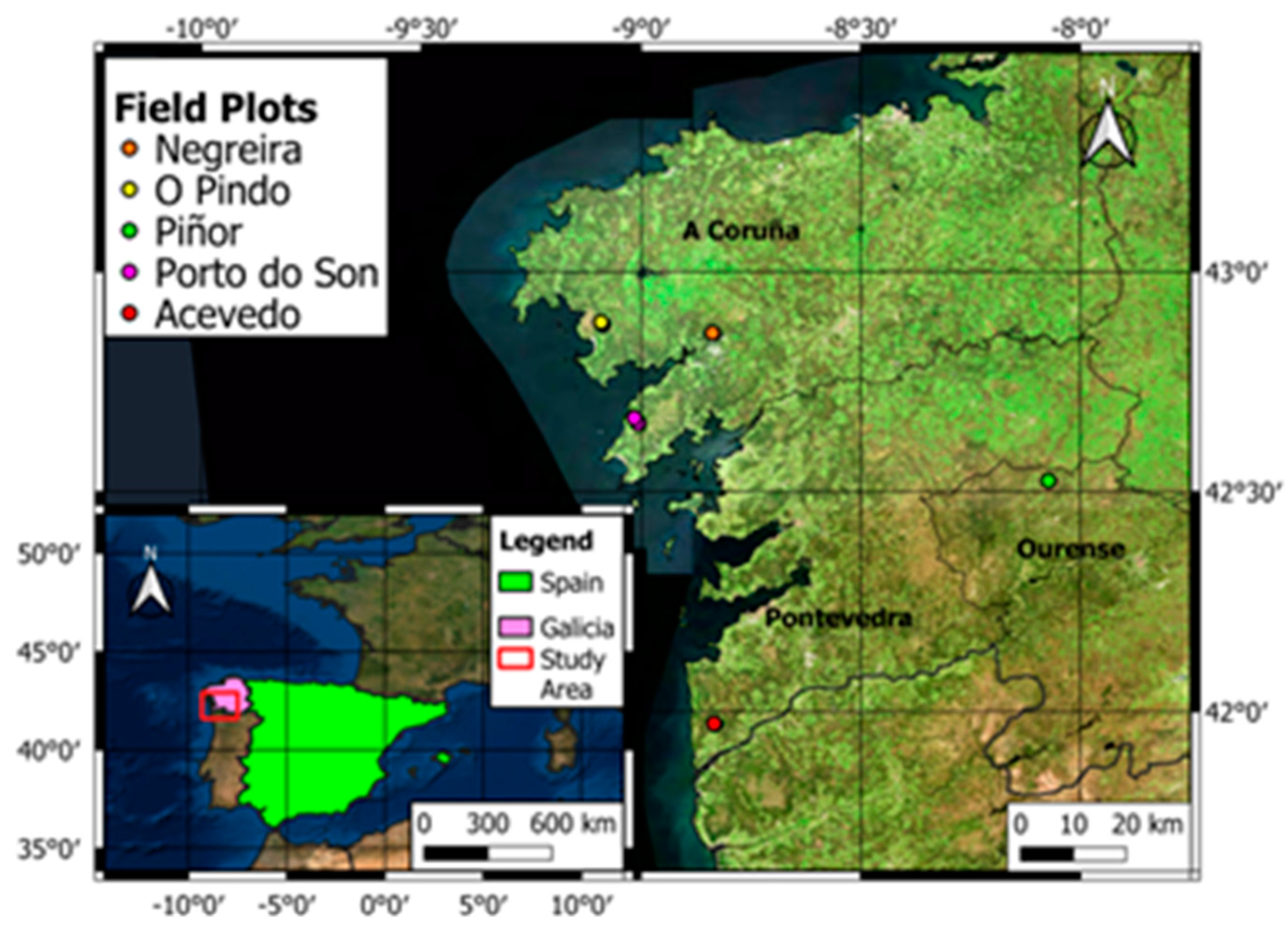
2.1. Study Area

The study was carried out in areas in Galicia affected by high-severity summer fires (vegetation was burned completely) between 2009 and 2016 to evaluate vegetation cover, with periods of regrowth of between 2.5 and 10 years after a fire. We focused on the plant communities dominated by gorse (Ulex europaeus L.). These shrublands are the dominant vegetation communities in the study area and are usually affected by summer fires. The usual fire season in the area is summer (July to October). Five experimental sites (Figure 1) were delineated, with at least two plots per site. A minimum distance of 1000 m between plots was applied to prevent autocorrelation or spatial autocorrelation in the data [40]. Twenty-two plots were established within the burned areas, and the coordinates of the locations were determined. Information about each experimental site is included in Table 1.

2.2. Layout of Experimental Plots and Characterization of Vegetation

The experimental plots were installed in homogeneous areas of shrubland dominated by Ulex europaeus L. Vegetation variables were assessed by a combination of non-destructive measurement of structural variables (height and cover transect) and destructive sampling of small plots. The central coordinates of the plots were established, and the plots were located in the field with the aid of an RTK-GPS equipment. The reference positions were marked in the field with a graduated rod.
Two transects of 20 m lengths were established in each plot, and plant cover was estimated using the line intercept method [41]. The direction of the first transect was defined by the position of the minute hand of a watch at that moment. The second transect was established perpendicular to the first one. Cover and height of all plant species were recorded along each transect (Figure 2). Fieldwork and laboratory work were carried out in the spring and summer of 2019.
Destructive sampling was carried out in 4 m2 square subplots, one within each sampling plot. All the standing vegetation material within the subplots was clipped and transported to the laboratory. The material was subsequently classified into thickness size classes (0–6 mm, 6–25 mm, 25–75 mm, and >75 mm), with the aid of calipers, and the physiological state (live/dead) was recorded, before the material was oven-dried at 105 ºC for 24 h and weighed to determine the dried mass.
The combined field and laboratory measurements enabled estimation of shrub cover (%), shrub height (cm), total standing biomass (kg/m2), and the fractions of: live fine biomass (kg/m2), dead fine biomass (kg/m2), total live biomass (kg/m2) and total dead biomass (kg/m2). These variables are usually used to assess fuel characteristics and potential fire behavior, but they can also be used to detect areas where vegetation cover is not sufficient to protect the soil through natural regeneration following a disturbance.

2.3. Explanatory Variables

A combination of remotely sensed data (LiDAR and multispectral imagery) was used to assess the vegetation structure. LiDAR data was accessed from the Plan BásicoAutonómico (Xunta de Galicia) [42] and used to compute the variables related to fuel cover, height, and load in the study areas. The LiDAR flight took place in 2019 (4 return points m−2). Multispectral imagery from the Sentinel-2 program was used to generate the set of spectral indexes potentially related to vegetation recovery.
Data were generated for the present study by processing the LiDAR and Sentinel-2 data independently, and both sources were combined in the regression analysis (Figure 3). The LiDAR data were processed using FUSION software [43]. A Digital Surface Model (DSM) was constructed by using Ground Filter (filtering of the point cloud to identify, using height thresholds, the points corresponding to gorse shrubland) and Grid Surface Create (creation of a raster DSM from the filtered point cloud using Ground Filter) tools and clipped for each of the plots measured in situ (ClipData tool), using the central coordinates and a radius of 10 m, covering the same area as field plots. Based on the correlation matrix between field data and raw LiDAR metrics, the mean, maximum, and minimum heights (Emean, Emax, Emin) and several height percentiles (E1, E5, E10, E20, E30, E40, E50, E60, E70, E75, E90) were chosen as predictors for estimating post-fire vegetation variables in the field.
The Sentinel-2 images were processed using R software [44]. Once Sentinel-2 images were pre-processed, the vegetation was resampled (from 20 to 10 m) and cropped as close as possible to the study area to reduce the processing time. A total of four Sentinel-2 tiles were downloaded and examined to determine the available sensing date as close as possible to the time of field sampling (Acevedo: tile 29TNG and sensing date 19 February 2019; Negreira: tile 29TNH and sensing date 29 March 2019; Pindo: tile 29TMH and sensing date 14 November 2018; Porto do Son: tile 29TMH and sensing date 08 January 2019; Piñor: tile 29TNH and sensing date 18 June 2019). All the images were downloaded already atmospherically, radiometrically, and geometrically corrected (Level-2A) by the Sen2Cor algorithm. Sen2Cor performed a pre-processing of Level-1C (L1C) Top of Atmosphere (TOA) image data, and applied a scene classification, an atmospheric correction, and a subsequent conversion into an ortho-image Level-2A Bottom-Of-Atmosphere (BOA) reflectance product [45,46]. Although the presence of clouds was checked prior to downloading the images, removal of pixels classified as clouds was ensured using the Scene Classification Image (SCL) mask. A list of spectral bands (Table 2) was used to calculate spectral indices. Once Sentinel-2 images were pre-processed, different spectral indices related to the physiological activity of vegetation were obtained according to their usefulness for fuel load estimation (Table 3). Once the spectral indices were calculated, the mean value of each index and for each plot was extracted with QGIS software. The information was cropped to the 10-m buffer generated around the center of each plot, defined by its coordinates, to match the area covered by LiDAR data.

2.4. Statistical Analysis

Measurements of post-fire vegetation structure and remote-sensed variables were used to construct statistical models for vegetation variables. A total of 19 independent variables were included in the statistical analysis. Exponential regression was used to evaluate the capacity of the independent variables to predict the shrub characteristics, as is usual in biomass modelling based on remote sensing [36,52,53].The exponential regression models presented were fitted to linear regression models, with the last term of the equation being the bias corrector.
The performance of the predictive models was assessed with the following metrics: adjusted R2, which is a modified version of R2 adjusted according to the number of predictors in the model; Root Mean Squared Error (RMSE), which measures the error of the prediction model as the average difference between the observed known values of the outcome and the value predicted by the model; and the Relative Root Mean Squared Error (RRMSE), a complement of the RMSE that measures the percentage of the RMSE with respect to the mean value of the dependent variable.
Adjusted models were tested to determine whether they fulfilled the Ordinary Least Squares assumptions: absence of multicollinearity between independent variables, linearity of the data in the relationship between independent and dependent variables, normality of residuals, and homogeneity of residuals variance with a mean of 0 (homoscedasticity). Possible multicollinearity was evaluated by the tolerance parameter (TOL). When multicollinearity was indicated (TOL < 0.1), problematic predictors were eliminated. Potential errors due to the lack of linearity of the data or the lack of normality and homogeneity of residuals were addressed by examination of plots of residuals vs. fitted values, normal Q-Q, scale-location, and residuals vs. leverage. The R statistical software [44] was used to perform the analysis. The R variable selection method “both”, a combination of “forward” and “backward” methods, was used to select the regressor variables.

3. Results

The main characteristics of the shrublands under study, which were determined in field inventories and laboratory analyses, are listed in Table 4. In all cases, the vegetation completely covered the soil, with maximum values over 300%. The range of variation of vegetation height was higher than that observed for vegetation cover, with the highest value being four times greater than the lowest value. The total standing biomass was also highly variable, with the highest amount being five times that of the lowest amount. Live portions of vegetation represented on average 77% of the total standing biomass. The fine standing biomass represented 65% of the total standing biomass, and the dead fraction accounted for only 23% of the total. Dead standing biomass was eight times greater and the dead fine biomass up to 16 times higher in the older communities.
The mean values and range of Sentinel-2 spectral indices are shown in Table 5. The Ratio Vegetation Index displayed the highest range of variation. The values of the SAVI and EVI indices were very similar.
The LiDAR metrics used to estimate shrub height are listed in Table 6. The 60th to 90th percentiles indicated similar differences between the lowest and the highest values.
The multiple exponential regression models for all the vegetation variables, determined using Sentinel-2 spectral indices, are compiled in Table 7.
The models obtained ranged from an adjusted r2 of 0.4 for vegetation height to 0.7 for total dead biomass. In the latter model, the explanatory variables were NBR and NDVI. The other models showed similar levels of fit. NBR was the most frequent index included in all models, except for total standing biomass. EVI and SAVI were the next most frequent and were included in all models except for vegetation cover and total dead biomass.
The multiple exponential regression models determined using LiDAR metrics are shown in Table 8. The models, including LiDAR data, performed better for explaining the variability in vegetation height and cover and for dead fine biomass than those shown in Table 7. The first percentile and the 50th to 75th percentiles represented the explanatory variables in these models.
In most cases, the best results were obtained with the combined data from Sentinel-2 and LiDAR metrics (Table 9 and Figure 4). The highest correlation was obtained for the total standing biomass. The only exception was total live biomass. RVI was the only spectral index in the total standing biomass and dead fine biomass models.

4. Discussion

Evaluation of forest vegetation biomass or growth is frequently carried out in remote sensing research; however, further information is needed about post-fire regrowth [34,35], particularly to aid studies using models to predict different vegetation characteristics [2]. Several studies have assessed the recovery or growth of AGB over areas of very different extensions; however, not all of these studies are supported by detailed field data [8,35,54,55]. There remains a need to have field data available to validate and calibrate remote sensing data sources [31,38]. To our knowledge, no previous studies have modelled the different shrub fractions (dead/live or fine/total biomass), and very few have considered biomass and strata (herbaceous/shrub) separately [56]. It is particular important to be able model the fraction of thin and dead standing AGB as input for a dynamic evaluation of fire hazard through changes in the prediction of potential fire behavior in those vegetation communities [23]. The results presented in this study show the potential of the combined use of LiDAR and Sentinel-2 spectral indices to obtain specific parameters to describe shrubland complexes and obtain inputs to be used in fire behavior simulator programs. With the values obtained in this study, it can be seen that the values of total fuel load or dead fuel load reached the upper range of these communities six years after the fire [21]. Three years after the fire, although the vegetation cover was 100%, only 33% of the pre-fire load had been reached.
The NDVI is undoubtedly one of the most commonly used vegetation indexes [8,16,32,54,55,57], and it is considered one of the best performing indexes as regards accounting for the variability of vegetation, especially in densely vegetated areas [57]. However, in the present study it only made a large contribution in two of the regression models. By contrast, the Normalized Burned Ratio (NBR) was one of the most important indices in the obtained models. One possible explanation for the low level of importance of the NDVI for explaining the shrub characteristics in our models may be the saturation of the index in scenarios of large quantities of biomass [58], which reached up to 70 t/ha in our study. Observations by Lu et al. [31] showed that indices including near-infrared information showed weaker correlations with AGB than those based on shortwave infrared in sites presenting a complex vegetation structure. Although NBR has been less commonly used to assess vegetation characteristics, its capacity to characterize vegetation AGB has been observed in previously published research [35,59,60,61,62,63]. The preference for other indexes rather than NDVI to assess AGB in shrublands is not a new finding. For example, Chen et al. (2018) [53] modelled AGB in semi-arid ecosystems with the Ratio Vegetation Index (RVI) and brightness.
The addition of LiDAR data to optical multispectral RS greatly increased the capacity of the method to determine standing AGB, as previously pointed out by several authors [4,35,53]. Our results regarding the independent variables selected were consistent with and confirm previous findings. Remote sensing optical imagery is considered more suitable for assessing the horizontal distribution of vegetation, whereas LiDAR data performs better for modelling the vertical structure of the vegetation [31,35,64]. In this respect, for characteristics related to vertical structure or AGB indicators, optical vegetation indexes played a secondary role, and the most important variables were those extracted from LiDAR metrics. This was previously demonstrated by Zolkos et al. (2013) [65], who performed a meta-analysis of more than 70 articles on AGB assessment from RS sources and demonstrated that the inclusion of LiDAR metrics significantly improved the performance of AGB models. Similarly, other studies combining several data sources have observed that Synthetic Aperture Radar (SAR) performs better than optical remote sensing data (NDVI), although the combination of both data sources improved the adjusted AGB models [36].
The results obtained in the present study show that structural characterization with LiDAR and satellite data can give good results. However, this methodology should be tested in more shrubland communities, and with a wider temporal range. The possibility of further studies is also limited by the acquisition of LiDAR data.

5. Conclusions

The study addressed the structural characterization of gorse shrublands in north-western Spain, and models were constructed for predicting the different characteristics (height, cover, total standing AGB and AGB by thickness fraction and physiological condition), with adjusted coefficients of determination ranging from 0.6 to 0.9. The addition of LiDAR data to optical RS images greatly improved the model performance, especially in relation to the vertical structure of the shrub complex. The models were derived from post-fire vegetation data, covering a period of between 2 and 10 years after the fire. Future research should focus on calibrating the models in other areas and, when necessary, should include new vegetation communities at different moments after the fire.
Our findings are sufficiently robust to be potentially applied in forest management plans, as they enable shrub characteristics to be mapped using freely available data at a regional scale. The data present an adequate balance between spatial resolution (higher for PNOA LiDAR data) and temporal resolution (higher for Sentinel-2 mission). The models developed are potentially useful for assessing spatial fire hazards due to fuel build-up and for acting as carbon sinks.

Author Contributions

Conceptualization, J.M.F.-A., R.L., J.A.S. and C.F.; methodology, J.M.F.-A., R.L., J.A.S. and C.F.; formal analysis, J.M.F.-A., R.L., J.A.S. and C.F.; investigation, J.M.F.-A., R.L., J.A.S. and C.F.; writing–original draft, J.M.F.-A., R.L., J.A.S., A.D.R.-G., J.G.A.-G., J.A.V. and C.F.; data curation, J.M.F.-A., R.L., J.A.S., A.D.R.-G., J.G.A.-G., J.A.V. and C.F.; supervision, J.A.S., C.F.; project administration, J.A.S. and C.F.; funding acquisition, J.A.S. and C.F. All authors have read and agreed to the published version of the manuscript.

Funding

This research was funded by the EU Interreg-Sudoe program through project EPyRIS (SOE2/P5/E0811).

Data Availability Statement

The datasets used or analyzed during the current study will be made available upon reasonable request.

Conflicts of Interest

The authors declare no conflict of interest.

References

  1. Zheng, G.; Chen, J.M.; Tian, Q.J.; Ju, W.M.; Xia, X.Q. Combining remote sensing imagery and forest age inventory for biomass mapping. J. Environ. Manag. 2007, 85, 616–623. [Google Scholar] [CrossRef] [PubMed]
  2. IPCC. IPCC Guidelines for National Greenhouse Gas Inventories; Eggelston, S., Buendia, L., Miwa, K., Ngara, T., Tanabe, K., Eds.; IGES: Hayama, Japan, 2006. [Google Scholar]
  3. Meng, R.; Wu, J.; Schwager, K.L.; Zhao, F.; Dennison, P.E.; Cook, B.D.; Brewster, K.; Green, T.M.; Serbin, S.P. Using high spatial resolution satellite imagery to map forest burn severity across spatial scales in a Pine Barrens ecosystem. Remote Sens. Environ. 2017, 191, 95–109. [Google Scholar] [CrossRef] [Green Version]
  4. Meng, R.; Wu, J.; Zhao, F.; Cook, B.D.; Hanavan, R.P.; Serbin, S.P. Measuring short-term post-fire forest recovery across a burn severity gradient in a mixed pine-oak forest using multi-sensor remote sensing techniques. Remote Sens. Environ. 2018, 210, 282–296. [Google Scholar] [CrossRef]
  5. García, M.; Saatchi, S.; Casas, A.; Koltunov, A.; Ustin, S.L.; Ramirez, C.; Balzter, H. Extrapolating Forest Canopy Fuel Properties in the California Rim Fire by Combining Airborne LiDAR and Landsat OLI Data. Remote Sens. 2017, 9, 394. [Google Scholar] [CrossRef] [Green Version]
  6. Engelstad, P.S.; Falkowski, M.; Wolter, P.; Poznanovic, A.; Johnson, P. Estimating Canopy Fuel Attributes from Low-Density LiDAR. Fire 2019, 2, 38. [Google Scholar] [CrossRef] [Green Version]
  7. Kumar, L.; Mutanga, O. Remote Sensing of Above-Ground Biomass. Remote Sens. 2017, 9, 935. [Google Scholar] [CrossRef] [Green Version]
  8. Gouveia, C.; DaCamara, C.C.; Trigo, R.M. Post-fire vegetation recovery in Portugal based on spot/vegetation data. Nat. Hazards Earth Syst. Sci. 2010, 10, 673–684. [Google Scholar] [CrossRef] [Green Version]
  9. Gitas, I.; Mitri, G.; Veraverbeke, S.; Polychronaki, A. Advances in remote sensing of post-fire vegetation recovery monitoring—A review. In Remote Sensing Biomass Principles Applications; Fatoyinbo, L., Ed.; IntechOpen: London, UK, 2012; pp. 143–176. [Google Scholar]
  10. De Groot, W.J.; Flanagan, D.C.; Stocks, B.J. Climate change and wildfires. In Proceedings of the Fourth International Symposium on Fire Economics, Planning, and Policy: Climate Change and Wildfires, Albany, CA, USA, 5–11 November 2012; pp. 1–10. [Google Scholar]
  11. Camia, A.; Libertà, G.; San Miguel, J. Modeling the Impacts of Climate Change on Forest Fire Danger in Europe; Publications Office of the European Union: Luxembourg, 2017. [Google Scholar]
  12. Vega, J.; Fernández, C.; Arellano-Pérez, S.; Fonturbel, T.; Ruíz, A. Os incendios forestais do cambio global xa estan aquí. Un desafío e unha ocasión para lograr unha resposta social consensuada. In Unha Nova Xeración de Lumes? Díaz-Fierros, F., Ed.; Consello da Cultura Galega: Santiago de Compostela, Spain, 2021; pp. 51–119. [Google Scholar]
  13. San-Miguel-Ayanz, J.; Moreno, J.M.; Camia, A. Analysis of large fires in European Mediterranean landscapes: Lessons learned and perspectives. For. Ecol. Manag. 2013, 294, 11–22. [Google Scholar] [CrossRef]
  14. Flannigan, M.; Cantin, A.S.; de Groot, W.J.; Wotton, M.; Newbery, A.; Gowman, L.M. Global wildland fire season severity in the 21st century. For. Ecol. Manag. 2013, 294, 54–61. [Google Scholar] [CrossRef]
  15. San-Miguel-Ayanz, J.; Tracy, D.; Boca, R.; Libertà, G.; Branco, A.; de Rigo, D.; Ferrari, D.; Maianti, P.; Artés Vivancos, T.; Costa, H.; et al. Forest Fires in Europe, Middle East and North Africa 2017; Joint Research Center, European Union: Ispra, Italy, 2018. [Google Scholar]
  16. Aranha, J.; Enes, T.; Calvão, A.; Viana, H. Shrub Biomass Estimates in Former Burnt Areas Using Sentinel 2 Images Processing and Classification. Forests 2020, 11, 555. [Google Scholar] [CrossRef]
  17. Ministerio de Medio Ambiente y Medio Rural yMarino. Cuarto Inventario Forestal Nacional; Ministerio de Medio Ambiente y Medio Rural yMarino: Galicia, Spain, 2011. [Google Scholar]
  18. Calvo, L.; Baeza, J.; Marcos, E.; Santana, V.M.; Papanastasis, V.P. Post-fire management of shrublands. In Post-Fire Management and Restoration of Southern European Forests; Moreira, F., Arianoutsou, M., Corona, P., De las Heras, J., Eds.; Managing Forest Ecosystems; Springer: Berlin/Heidelberg, Germany, 2012; Volume 24, pp. 293–319. [Google Scholar]
  19. CMR. Plan de Prevención y Defensa Contra los Incendios Forestales de Galicia; Xunta de Galicia: Santiago, Spain, 2022; p. 259.
  20. Botequim, B.; Zubizarreta-Gerendiain, A.; Garcia-Gonzalo, J.; Silva, A.; Marques, S.; Fernandes, P.; Pereira, J.; Tomé, M. A model of shrub biomass accumulation as a tool to support management of Portuguese forests. Iforest Biogeosci. For. 2015, 8, 114–125. [Google Scholar] [CrossRef] [Green Version]
  21. Vega, J.A.; Arellano-Pérez, S.; Álvarez-González, J.G.; Fernández, C.; Jiménez, E.; Fernández-Alonso, J.M.; Vega-Nieva, D.J.; Briones-Herrera, C.; Alonso-Rego, C.; Fontúrbel, T.; et al. Modelling aboveground biomass and fuel load components at stand level in shrub communities in NW Spain. For. Ecol. Manag. 2022, 505, 119926. [Google Scholar] [CrossRef]
  22. Fernández, C.; Vega, J.A. Shrub recovery after fuel reduction treatments in a gorse shrubland in northern Spain. J. Environ. Manag. 2016, 166, 211–216. [Google Scholar] [CrossRef] [PubMed]
  23. Keane, R.E. Wildland Fuel Fundamentals and Applications; Springer: Berlin/Heidelberg, Germany, 2015; p. 191. [Google Scholar]
  24. Finney, M.A. FARSITE: Fire Area Simulator-Model Development and Evaluation; U.S. Department of Agriculture, Forest Service; Volume Research Paper RMRS-RP-4; Rocky Mountain Research Stationort: Collins, CO, USA, 1998.
  25. Keane, R.E. Describing wildland surface fuel loading for fire management: A review of approaches, methods and systems. Int. J. Wildland Fire 2013, 22, 51–62. [Google Scholar] [CrossRef]
  26. Baeza, M.J.; Raventós, J.; Escarré, A.; Vallejo, V.R. Fire Risk and Vegetation Structural Dynamics in Mediterranean Shrubland. Plant Ecol. 2006, 187, 189–201. [Google Scholar] [CrossRef]
  27. Marino, E.J.M.; Guijarro, M.C.H.; Díez, C.; Fernández, C. Flammability descriptors of fine dead fuels resulting from two mechanical treatments in shrubland: A comparative laboratory study. Int. J. Wildland Fire 2010, 19, 314–324. [Google Scholar] [CrossRef]
  28. Fernández, C. Medium-term effects of straw helimulching on post-fire vegetation recovery in shrublands in north-west Spain. Int. J. Wildland Fire 2021, 30, 301–305. [Google Scholar] [CrossRef]
  29. Madrigal, J.; Marino, E.; Guijarro, M.; Hernando, C.; Díez, C. Evaluation of the flammability of gorse (Ulex europaeus L.) managed by prescribed burning. Ann. For. Sci. 2012, 69, 387–397. [Google Scholar] [CrossRef] [Green Version]
  30. Kumar, L.; Sinha, P.; Taylor, S.; Alqurashi, A. Review of the use of remote sensing for biomass estimation to support renewable energy generation. J. Appl. Remote Sens. 2015, 9, 097696. [Google Scholar] [CrossRef]
  31. Lu, D.; Chen, Q.; Wang, G.; Liu, L.; Li, G.; Moran, E. A survey of remote sensing-based aboveground biomass estimation methods in forest ecosystems. Int. J. Digit. Earth 2016, 9, 63–105. [Google Scholar] [CrossRef]
  32. Viana, H.; Aranha, J.; Lopes, D.; Cohen, W.B. Estimation of crown biomass of Pinus pinaster stands and shrubland above-ground biomass using forest inventory data, remotely sensed imagery and spatial prediction models. Ecol. Model. 2012, 226, 22–35. [Google Scholar] [CrossRef]
  33. Mutanga, O.; Shoko, C.; Adelabu, S.; Bangira, T. Remote sensing of aboveground forest biomass: A review. Trop. Ecol. 2016, 57, 125–132. [Google Scholar]
  34. Durante, P.; Martín-Alcón, S.; Gil-Tena, A.; Algeet, N.; Tomé, J.L.; Recuero, L.; Palacios-Orueta, A.; Oyonarte, C. Improving Aboveground Forest Biomass Maps: From High-Resolution to National Scale. Remote Sens. 2019, 11, 795. [Google Scholar] [CrossRef] [Green Version]
  35. Wulder, M.A.; White, J.C.; Alvarez, F.; Han, T.; Rogan, J.; Hawkes, B. Characterizing boreal forest wildfire with multi-temporal Landsat and LIDAR data. Remote Sens. Environ. 2009, 113, 1540–1555. [Google Scholar] [CrossRef]
  36. Vaglio, G.; Pirotti, F.; Callegari, M.; Chen, Q.; Cuozzo, G.; Lingua, E.; Notarnicola, C.; Papale, D. Potential of ALOS2 and NDVI to Estimate Forest Above-Ground Biomass, and Comparison with Lidar-Derived Estimates. Remote Sens. 2017, 9, 18. [Google Scholar] [CrossRef] [Green Version]
  37. Sun, G.; Ranson, K.J. Forest biomass retrieval from lidar and radar. In Proceedings of the 2009 IEEE International Geoscience and Remote Sensing Symposium, Cape Town, South Africa, 12–17 July 2009; pp. V-300–V-303. [Google Scholar]
  38. Kellner, J.R.; Armston, J.; Birrer, M.; Cushman, K.C.; Duncanson, L.; Eck, C.; Falleger, C.; Imbach, B.; Král, K.; Krůček, M.; et al. New Opportunities for Forest Remote Sensing Through Ultra-High-Density Drone Lidar. Surv. Geophys. 2019, 40, 959–977. [Google Scholar] [CrossRef] [Green Version]
  39. Tang, H.; Armston, J.; Hancock, S.; Marselis, S.; Goetz, S.; Dubayah, R. Characterizing global forest canopy cover distribution using spaceborne lidar. Remote Sens. Environ. 2019, 231, 111262. [Google Scholar] [CrossRef]
  40. Bataineh, A.L.; Oswald, B.P.; Bataineh, M.; Unger, D.; Hung, I.K.; Scognamillo, D. Spatial autocorrelation and pseudoreplication in fire ecology. Fire Ecol. 2006, 2, 107–118. [Google Scholar] [CrossRef]
  41. Canfield, R.H. Application of the Line Interception Method in Sampling Range Vegetation. J. For. 1941, 39, 388–394. [Google Scholar] [CrossRef]
  42. XdG. Plan Básico Autonómico. Available online: http://mapas.xunta.gal (accessed on 3 December 2021).
  43. McGaughey, R.J. FUSION/LDV: Software for LiDAR Data Analysis and Visualization; US Department of Agriculture, Forest Service, Pacific Northwest Research Station: Seattle, WA, USA, 2009.
  44. Core Team Development, R. R: A Language and Environment for Statistical Computing; R Foundation for Statistical Computing: Vienna, Austria, 2022. [Google Scholar]
  45. Kaufman, Y.J.; Sendra, C. Algorithm for automatic atmospheric corrections to visible and near-IR satellite imagery. Int. J. Remote Sens. 1988, 9, 1357–1381. [Google Scholar] [CrossRef]
  46. Copernicus, H. Copernicus Open Access Hub. Available online: https://scihub.copernicus.eu/dhus/#/home (accessed on 24 February 2022).
  47. Key, C.H.; Benson, N.C. Landscape Assessment: Ground Measure of Severity, the Composite Burn Index; and Remote Sensing of Severity, the Normalized Burn Ratio; RMRS-GTR-164-CD: LA 1-51; USDA Forest Service, Rocky Mountain Research Station: Odgen, UT, USA, 2006.
  48. Rouse, J.W.; Haas, R.H.; Schell, J.A.; Deering, D.W. Monitoring vegetation systems in the Great Plains with ERTS. In Proceedings of the Third Earth Resources Technology Satellite–1 Symposium, Washington, DC, USA, 10–14 December 1973; pp. 309–317. [Google Scholar]
  49. Jordan, C.F. Derivation of Leaf-Area Index from Quality of Light on the Forest Floor. Ecology 1969, 50, 663–666. [Google Scholar] [CrossRef]
  50. Huete, A.R. A soil-adjusted vegetation index (SAVI). Remote Sens. Environ. 1988, 25, 295–309. [Google Scholar] [CrossRef]
  51. Liu, H.Q.; Huete, A. A feedback based modification of the NDVI to minimize canopy background and atmospheric noise. IEEE Trans. Geosci. Remote Sens. 1995, 33, 457–465. [Google Scholar] [CrossRef]
  52. Xu, B.; Gong, P.; Pu, R. Crown closure estimation of oak savannah in a dry season with Landsat TM imagery: Comparison of various indices through correlation analysis. Int. J. Remote Sens. 2003, 24, 1811–1822. [Google Scholar] [CrossRef]
  53. Chen, W.; Zhao, J.; Cao, C.; Tian, H. Shrub biomass estimation in semi-arid sandland ecosystem based on remote sensing technology. Glob. Ecol. Conserv. 2018, 16, e00479. [Google Scholar] [CrossRef]
  54. Meng, R.; Dennison, P.E.; Huang, C.; Moritz, M.A.; D’Antonio, C. Effects of fire severity and post-fire climate on short-term vegetation recovery of mixed-conifer and red fir forests in the Sierra Nevada Mountains of California. Remote Sens. Environ. 2015, 171, 311–325. [Google Scholar] [CrossRef]
  55. Yang, J.; Pan, S.; Dangal, S.; Zhang, B.; Wang, S.; Tian, H. Continental-scale quantification of post-fire vegetation greenness recovery in temperate and boreal North America. Remote Sens. Environ. 2017, 199, 277–290. [Google Scholar] [CrossRef]
  56. Li, A.; Dhakal, S.; Glenn, N.F.; Spaete, L.P.; Shinneman, D.J.; Pilliod, D.S.; Arkle, R.S.; McIlroy, S.K. Lidar Aboveground Vegetation Biomass Estimates in Shrublands: Prediction, Uncertainties and Application to Coarser Scales. Remote Sens. 2017, 9, 903. [Google Scholar] [CrossRef] [Green Version]
  57. Veraverbeke, S.; Gitas, I.; Katagis, T.; Polychronaki, A.; Somers, B.; Goossens, R. Assessing post-fire vegetation recovery using red–near infrared vegetation indices: Accounting for background and vegetation variability. ISPRS J. Photogramm. Remote Sens. 2012, 68, 28–39. [Google Scholar] [CrossRef] [Green Version]
  58. Huete, A.; Didan, K.; Miura, T.; Rodriguez, E.P.; Gao, X.; Ferreira, L.G. Overview of the radiometric and biophysical performance of the MODIS vegetation indices. Remote Sens. Environ. 2002, 83, 195–213. [Google Scholar] [CrossRef]
  59. Escuin, S.; Navarro, R.; Fernández, P. Fire severity assessment by using NBR (Normalized Burn Ratio) and NDVI (Normalized Difference Vegetation Index) derived from LANDSAT TM/ETM images. Int. J. Remote Sens. 2008, 29, 1053–1073. [Google Scholar] [CrossRef]
  60. Li, A.; Huang, C.; Sun, G.; Shi, H.; Toney, C.; Zhu, Z.; Rollins, M.G.; Goward, S.N.; Masek, J.G. Modeling the height of young forests regenerating from recent disturbances in Mississippi using Landsat and ICESat data. Remote Sens. Environ. 2011, 115, 1837–1849. [Google Scholar] [CrossRef]
  61. Pascual, C.; García-Abril, A.; Cohen, W.B.; Martín-Fernández, S. Relationship between LiDAR-derived forest canopy height and Landsat images. Int. J. Remote Sens. 2010, 31, 1261–1280. [Google Scholar] [CrossRef]
  62. Vargas-Larreta, B.; López-Sánchez, C.A.; Corral-Rivas, J.J.; López-Martínez, J.O.; Aguirre-Calderón, C.G.; Álvarez-González, J.G. Allometric Equations for Estimating Biomass and Carbon Stocks in the Temperate Forests of North-Western Mexico. Forests 2017, 8, 269. [Google Scholar] [CrossRef] [Green Version]
  63. Nguyen, T.H.; Jones, S.; Soto-Berelov, M.; Haywood, A.; Hislop, S. A Comparison of Imputation Approaches for Estimating Forest Biomass Using Landsat Time-Series and Inventory Data. Remote Sens. 2018, 10, 1825. [Google Scholar] [CrossRef] [Green Version]
  64. Alonso-Rego, C.; Arellano-Pérez, S.; Cabo, C.; Ordoñez, C.; Álvarez-González, J.G.; Díaz-Varela, R.A.; Ruiz-González, A.D. Estimating Fuel Loads and Structural Characteristics of Shrub Communities by Using Terrestrial Laser Scanning. Remote Sens. 2020, 12, 3704. [Google Scholar] [CrossRef]
  65. Zolkos, S.G.; Goetz, S.J.; Dubayah, R. A meta-analysis of terrestrial aboveground biomass estimation using lidar remote sensing. Remote Sens. Environ. 2013, 128, 289–298. [Google Scholar] [CrossRef]
Figure 1. Location of the experimental sites within Galicia (NW Spain) affected by fires between 2009 and 2016. The reference coordinate system is WGS84 (EPSG: 4326).
Remotesensing 14 06063 g001
Figure 2. Partial view of a sampling plot six years after a fire.
Remotesensing 14 06063 g002
Figure 3. Flowchart of processing steps using LiDAR, Sentinel-2 and field data.
Remotesensing 14 06063 g003
Figure 4. Observed and predicted values of the variables under study using LiDAR and Sentinel-2 metrics. Red line corresponds to diagonal line and blue line correspond to trend line.
Remotesensing 14 06063 g004
Table 1. Characteristics of the experimental sites.
Experimental SiteMean Annual Precipitation (mm)Mean Annual Temperature °CAspectElevation
(m a.s.l)
Fire
Occurrence Date
Burned Area (ha)Number of Plots
Piñor124111.7W850September 20093502
Acevedo157214.5E275August 201318246
O Pindo94614.4W225September 201321665
Negreira145012.4W-SW240September 20136465
Porto do Son130014.6NE215August 20168704
Table 2. Sentinel-2 spectral bands.
Sentinel-2 BandsCentral Wavelength (μm)Resolution (m)
B2–Blue0.49010
B3–Green0.56010
B4–Red0.66510
B5 - Vegetation Red Edge0.70520
B6 - Vegetation Red Edge0.74020
B7 - Vegetation Red Edge0.78320
B8–NIR0.84210
B8A - Vegetation Red Edge0.86520
B10 - SWIR–Cirrus1.37560
B11–SWIR1.61020
B12–SWIR2.19020
Table 3. Sentinel-2 spectral indices used in the study.
IndexDescriptionAlgorithmReference
NBRNormalized Burn Ratio ( B 8 B 12 ) ( B 8 + B 12 ) [47]
NDVINormalized Difference Vegetation Index ( B 8 B 4 ) ( B 8 + B 4 ) [48]
RVIRatio Vegetation Index B 8 B 4 [49]
SAVISoil-Adjusted Vegetation Index ( B 8 B 4 ) ( B 8 + B 4 + L ) * ( 1 + L )
L = 0.5
[50]
EVIEnhanced Vegetation Index 2.5 * ( B 8 B 4 ) ( B 8 + 6 * B 4 7.5 * B 2 ) + 1 [51]
Table 4. Mean and range of variation of post-fire vegetation variables measured in the field plots.
Vegetation VariableMeanRange
Total cover, %220.0102.0–321.8
Height, cm105.845.0–190.0
Total standing biomass, kg/m23.11.1–5.9
Total live biomass, kg/m22.40.9–4.4
Total dead biomass, kg/m20.70.2–1.6
Live fine (diameter < 6 mm) biomass, kg/m21.40.9–2.8
Dead fine (diameter < 6 mm) biomass, kg/m20.60.1–1.6
Table 5. Mean and range of Sentinel-2 spectral indices used in the study.
Sentinel-2 Spectral IndexMeanRange
Normalized burn ratio (NBR)0.50.3–0.6
Normalized Difference Vegetation Index (NDVI)0.70.6–0.8
Ratio Vegetation Index (RVI)6.73.8–11.0
Soil-Adjusted Vegetation Index (SAVI)0.40.3–0.4
Enhanced Vegetation Index (EVI)0.40.3–0.4
Table 6. Mean and range variation of LiDAR metric values (cm) used in the gorse shrubland studied.
LiDAR Metrics (cm)MeanRange
Mean height (Emean)40.940.3–60.4
Maximum height (Emax)190.2170.3–200.3
Minimum height (Emin)0.00.0–1
1st height percentile (E1)0.00.0–1
5th height percentile (E5)10.0–1
10th height percentile (E10)10.0–1
20th height percentile (E20)10.0–1
30th height percentile (E30)21–4
40th height percentile (E40)61–24
50th height percentile (E50)1640–56
60th height percentile (E60)5037–83
70th height percentile (E70)7962–100
75th height percentile (E75)9379–113
90th height percentile (E90)138124–153
Table 7. Summary of best regression models and the corresponding statistical metrics (Adjusted R2, RMSE and RRMSE) determined for each vegetation variable using Sentinel-2 spectral indices. The RMSE units are the same as those of the dependent variable.
Vegetation VariableRegression ModelAdj. R2RMSE RRMSE   ( R M S E y ¯ ) %
Cover
(%)
e x p ( 4.0 + 0.3 · G R V I + 3.5 · N B R 0.3 · R V I ) 0.6141.319.4
Height
(cm)
e x p ( 6.3 + 44.1 · E V I + 3.2 · N B R 52.3 · S A V I ) 0.4334.031.4
Total standing biomass (kg/m2) e x p ( 3.7 + 42.5 · E V I + 7.4 · N D V I 0.2 · R V I 50.2 · S A V I ) 0.620.825.3
Total live biomass (kg/m2) e x p ( 2.8 + 25.6 · E V I + 3.9 · N B R 35.3 · S A V I ) 0.610.523.0
Total dead biomass (kg/m2) e x p ( 5.0 + 17.2 · N B R 16.7 · N D V I ) 0.730.234.3
Live fine biomass (kg/m2) e x p ( 1.3 + 11.0 · E V I + 1.7 · N B R 15.8 · S A V I ) 0.620.18.1
Dead fine biomass (kg/m2) e x p ( 0.6 + 72.6 · E V I + 8.7 · N B R 0.2 · R V I 82.7 · S A V I ) · 1.1 0.640.249.0
Table 8. Summary of best regression models and the corresponding statistical metrics (Adjusted R2, RMSE and RRMSE) determined for each vegetation variable using LiDAR metrics. The RMSE units are the same as those of the dependent variable.
Vegetation VariableRegression ModelAdj. R2RMSE RRMSE   ( R M S E y ¯ ) %
Cover
(%)
e x p ( 2.3 + 11.7 · E 1 + 0.3 · E 75 0.1 · E 60 ) 0.8144.320.8
Height
(cm)
e x p ( 4.4 + 0.2 · E 50 ) · 1.1 0.6226.524.5
Total standing biomass (kg/m2) e x p ( 2.6 + 0.3 · E 40 + 19.1 · E 5 + 0.6 · E 75 0.4 · E 70 ) · 1.1 0.341.344.9
Total live biomass (kg/m2) e x p ( 4.5 + 7.7 · E m i n + 0.4 · E 90 ) 0.640.523.0
Total dead biomass (kg/m2) e x p ( 3.3 + 0.6 · E 40 + 25.6 · E 10 ) · 1.1 0.730.341.1
Live fine biomass (kg/m2) e x p ( 2.3 + 6.8 · E 20 + 0.13 · E 95 ) 0.420.536.2
Dead fine biomass (kg/m2) e x p ( 7.9 + 23.6 · E 1 + 1.5 · E 75 E 70 ) · 1.1 0.820.236.9
Table 9. Summary of best regression models and the corresponding statistical metrics (Adjusted R2, RMSE and RRMSE) determined for each vegetation variable using a combination of LiDAR metrics and Sentinel-2 spectral indices. The RMSE units are the same as those of the dependent variable.
Vegetation VariableRegression ModelAdj. R2RMSE RRMSE   ( R M S E y ¯ ) %
Cover
(%)
e x p ( 3.2 + 0.4 · E m e a n + 3.1 · N B R 0.2 · R V I ) 0.8226.612.4
Height
(cm)
e x p ( 6.3 + 0.35 · E 50 3 · N D V I ) 0.7226.024.1
Total standing biomass (kg/m2) e x p ( 1.6 + 0.8 · E 40 0.2 · R V I ) 0.910.414.2
Total live biomass (kg/m2) e x p ( 4.5 + 7.7 · E m i n + 0.4 · E 90 ) 0.640.523.0
Total dead biomass (kg/m2) e x p ( 1.8 + 0.6 · E 40 + 3.8 · N B R 6.4 · N D V I ) 0.740.120.0
Live fine biomass (kg/m2) e x p ( 1.5 + 0.8 · E 30 + 1.2 · N B R 5.0 · S A V I ) 0.820.17.4
Dead fine biomass (kg/m2) e x p ( 0.03 + 1.3 · E 40 0.3 · R V I ) · 1.1 0.810.243.7
Publisher’s Note: MDPI stays neutral with regard to jurisdictional claims in published maps and institutional affiliations.

