Technical Note

Data-Driven Seismic Impedance Inversion Based on Multi-Scale Strategy

1
The State Key Laboratory of Petroleum Resources and Prospecting, National Engineering Laboratory for Offshore Oil Exploration, China University of Petroleum (Beijing), Beijing 102249, China
2
Petroleum Exploration and Production Research Institute, China Petroleum & Chemical Corporation (SINOPEC), Beijing 102206, China
*
Author to whom correspondence should be addressed.
Remote Sens. 2022, 14(23), 6056; https://doi.org/10.3390/rs14236056
Submission received: 25 October 2022 / Revised: 26 November 2022 / Accepted: 28 November 2022 / Published: 29 November 2022
(This article belongs to the Special Issue Geophysical Data Processing in Remote Sensing Imagery)

Abstract

:
Seismic impedance inversion is one of the most commonly used techniques for reservoir characterization. High accuracy and high resolution seismic impedance is a prerequisite for subsequent reservoir interpretation. The data-driven approach offers the opportunity for accurate impedance prediction by establishing a nonlinear mapping between seismic data and impedance. However, existing data-driven methods take the raw seismic data directly as input, making it difficult for the network to learn high frequency weak signal information and resulting in low resolution inversion results. In order to mitigate the above issues, a data-driven seismic impedance inversion method based on multi-scale strategy is proposed. The method first obtains seismic data at different scales using frequency division techniques and do normalization on the extracted multi-scale data to ensure the consistency of the seismic signal energy in different frequency bands. The multi-scale seismic data will then be fed into the network, which helps the network to learn the high frequency information features more easily, and ultimately obtain higher resolution inversion results. We use the most commonly used convolutional neural network (CNN) as an example to demonstrate that the proposed multi-scale data-driven seismic impedance inversion method can improve the resolution of the inversion results. In addition, since the above seismic impedance inversion method is executed trace-by-trace, the f-x prediction filtering technique is introduced to improve the lateral continuity of the inversion results and obtain more geologically reliable impedance profiles. The validity of the proposed method is verified in the application of synthetic model data as well as an actual data set.

Graphical Abstract

1. Introduction

Seismic impedance, the product of density and seismic velocity, directly reflects the nature of subsurface rocks and can be used to indicate oil and gas, calculate reserves, and guide well placement, etc. Compared with the original seismic data, the impedance profile obtained by seismic impedance inversion methods eliminates the tuning effect and improves the vertical resolution of seismic data, which is an important parameter for reservoir prediction in the field of oil and gas exploration [1,2]. Accurate impedance parameters are a prerequisite for subsequent reservoir interpretation. The interpretation of complex and unconventional reservoirs places greater demands on impedance accuracy and resolution. However, from a mathematical point of view, seismic impedance inversion is an inverse problem and is ill-posed. Due to the limitations of incompleteness, noise, and wavelet band limitations of the observed data, multiple geological models can usually be obtained to match the observed data. Moreover, if the given data and the established geophysical-mathematical model do not perfectly match the actual geological model during the inversion process, the solution in the specific geological sense will not exist or the solution will be unstable. Because the Earth medium is complex and variable [3], it is often difficult to accurately establish the relationship between seismic data and subsurface model parameters with a limited number of geophysical parameters and associated mathematical physical models. Although the theory and technology of these seismic inversion methods have been continuously improved, they are not as effective as desired in practical reservoir prediction and lithology characterization [4,5,6,7,8,9,10,11].
Unlike traditional seismic impedance inversion based on a known physical model (i.e., model-driven inversion method), the data-driven inversion method does not require a known physical model as a prerequisite. Deep learning, currently one of the most popular data-driven algorithms, can use a given training dataset to learn a mapping function between the model space and the data space to solve the inverse problem. Deep learning methods, represented by convolutional neural network (CNN), have been very successful in many real-world areas, (e.g., computer vision, image recognition and natural language processing) benefiting from the increase in computing power and the continuous improvement of algorithms [12,13,14]. This has led to a boom in the application of deep learning methods in geophysics and has led to many promising results. For instance, Zhang, et al. [15] use convolutional neural network combined with wavelet transform to achieve lithology/fluid prediction from seismic data. Zhang, et al. [16] further introduce priori information containing Markov chain and Markov random field in deep learning-based lithology/fluid prediction to improve the continuity of the prediction results. Wu, et al. [17] use a single convolutional neural network to predict fault probabilities, strikes and dips. Bi, et al. [18] implement simultaneous 3D seismic horizon and fault interpretation based on the deep learning approach. Deep learning-based seismic horizon and fault interpretation techniques have greatly improved efficiency with no less accuracy than manual interpretation. Saad and Chen [19] propose a fully unsupervised deep learning method to accomplish the suppression of random noise in seismic data. Kaur, et al. [20] implement seismic data interpolation using deep learning with generative adversarial network.
In addition to the above applications, deep learning-based seismic inversion is also a hot topic of research. Das, et al. [21] predict a seismic impedance model from recorded normal-incidence seismic data based on the convolutional neural network. Li, et al. [22] propose an end-to-end seismic inversion network to achieve deep learning based seismic inversion. Puzyrev, et al. [23] compare the performance of different deep learning methods (e.g., convolutional neural network, recurrent neural network, and fully connected network) for velocity estimation and demonstrate the potential of data-driven methods for seismic inversion. Zhang, et al. [24] introduce the initial model in deep learning-based seismic inversion to achieve stable post-stack and pre-stack inversions using hybrid deep neural networks as an example. Kazei, et al. [25] utilize a convolutional neural network to compute seismic velocity using multiple common-mid-point gathers as input. Cao, et al. [26] develop a deep learning multi-parameter pre-stack seismic inversion method based on sparse reflection coefficient constraints. Zhang, et al. [27] combine the full-wave field simulation method and the deep learning method to obtain higher accuracy inversion results. These methods ignore the energy differences of seismic data in different frequency bands. When raw seismic data is fed directly into the network, the network has difficulty learning high frequency weak signal information resulting in low resolution inversion results.
The multi-scale inversion strategy is a good choice to make full use of the high frequency information. This method can effectively reduce the nonlinearity of the inverse problem and avoid the solution falling into local minima. Some scholars use the Hamming window, Wiener filter and wavelet transform to perform multi-scale decomposition of seismic data for full waveform inversion, which improves both the global convergence of the inversion and the resolution of the predicted subsurface parameters effectively [28,29,30,31]. Inspired by this, we introduce the multi-scale inversion strategy into deep learning-based seismic impedance inversion. In this paper, we propose to obtain seismic data with different scales using frequency division techniques and do normalization on the extracted multi-scale seismic data to ensure the consistency of the seismic signal energy in different frequency bands, which will then be used as input to the network so that the network can learn the high frequency information features more easily. Then, we validate the effectiveness of the multi-scale strategy using a convolutional neural network as the underlying network on synthetic model data and real case. In addition, since the proposed method performs seismic impedance inversion trace-by-trace, we further introduce the f-x predictive filtering technique to improve the lateral continuity of the inversion results and thus obtain more geologically reliable impedance profiles.
The main contribution of this paper is that a data-driven seismic impedance inversion method based on a multi-scale strategy is proposed to help the network learn high-frequency weak signal features more easily and thus improve the resolution of the inversion results. In addition, the f-x predictive filtering technique is introduced to improve the lateral continuity of the inversion results and obtain more geologically reliable impedance profiles. Meanwhile, the proposed method is compared with a data-driven method using raw seismic data as the input and a model-driven seismic impedance method. This paper is organized as follows: we begin with an introduction to the principles of training dataset construction, network building and f-x filtering. Next, we perform numerical experiments on the model and real data to verify the validity of the proposed method. Some conclusions and outlooks are reported in Section 4.

2. Methods

The proposed method still belongs to the category of supervised learning, where the training dataset and the network are two key factors. In this section, we first introduce traditional forward modeling based on known physical models to construct sufficient training datasets. Next, the multi-scale strategy and the proposed deep learning seismic impedance inversion method are reported. Then, a brief description of how the transfer learning strategy is introduced to extend the proposed method to field data with limited well-logs data is presented. Finally, we give a brief report on the principles of the f-x filtering technique.

2.1. Forward Model

The seismic signals in the post-stack profile can be modeled approximately by the convolution of seismic wavelet with reflection coefficients as follows:
s ( t ) = + w ( τ ) r ( t τ ) d τ + n ( t )
where s ( t ) represents synthetic post-stack seismogram, w ( τ ) is the seismic wavelet, r ( τ ) is the reflection coefficient, n ( t ) represents observation noise, t represents two-way travel time and τ denotes a point in time at a given moment. The reflection coefficient r ( τ ) can be generated by using the difference and summation operators on the impedance model, as expressed in Equation (2):
r ( t ) = z t + 1 z t z t + 1 + z t
where z t + 1 and z t represent the seismic impedance of the layer t + 1 and t , respectively. Given the impedance model and seismic wavelet, the corresponding synthetic seismic records can be calculated by combining Equations (1) and (2). Then, most deep learning based seismic impedance inversion methods take synthetic seismic data as input and impedance models as output and combined with optimization algorithms can build a mapping function to achieve conversion of seismic data to impedance. Although this is an effective method, this ignores the energy differences in different frequency bands in the seismic data, increasing the difficulty for the network to learn the information of weak signals at high frequency, thus leading to insufficient resolution of the inversion results.

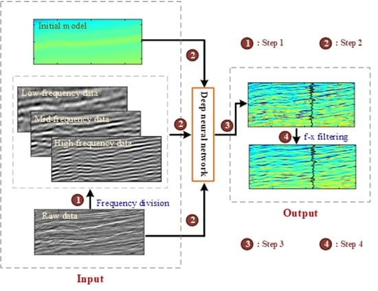
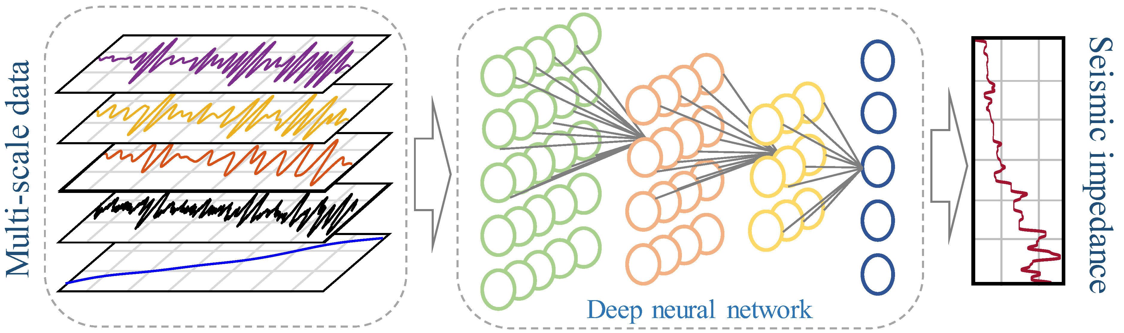
2.2. Inversion Framework of Multi-Scale Strategy

Figure 1 shows the schematic diagram of multi-scale seismic data extraction. Take a three-layer model containing two reflective interfaces as an example. When the synthesized signal (yellow curve shown in Figure 1a) contains both a strong energy low frequency signal (sky blue curve shown in Figure 1a) and a low energy high frequency signal (red curve in Figure 1a), it can be seen that it is almost impossible to distinguish the position of the interface in the synthesized signal (yellow curve shown in Figure 1a). In other words, if we take that synthesized signal as the input of the network, it is difficult for the network to learn the features of the high frequency information at that point. In order to decrease the difficulty of the network to learn high frequency information features, it is necessary to separate the data in different frequency bands from the synthesized signal. Figure 2 shows the amplitude spectrum corresponding to the synthesized signal (yellow curve shown in Figure 1a). It can be seen that the signal of different frequency bands in the amplitude spectrum can be well separated. Therefore, we split the amplitude spectrum of the signal with different windows (green dashed lines shown in Figure 1b) and obtain the multi-scale seismic data by inverse Fourier transform, as shown in Figure 1c. It can be seen that the extracted multi-scale seismic data can match well with the low and high frequency signals contained in the original synthetic signal. After obtaining the multiscale seismic data, we normalize the different frequency band data to ensure that the contribution of different frequency band signals in the network learning process is the same. This can improve the effectiveness of the network for feature extraction of high-frequency signals and improve the resolution of the final prediction results.
Based on the above strategy, we can obtain multi-scale seismic data in different frequency bands from the original seismic data. In this paper, multi-scale seismic data is extracted from the original seismic data in three frequency bands, called low-frequency, mid-frequency and high-frequency seismic data, respectively. It is worth noting that when extracting high-frequency seismic data, the high cut-off frequency does not exceed 80 Hz to prevent high frequency noise from interfering with the results. Different high cutoff frequency will be set for different data based on the main frequency of the seismic data. Low-frequency initial model is a kind of data often used in conventional seismic impedance inversion methods, which can compensate the problem of insufficient low-frequency information in seismic data and, at the same time, can reduce the multi-solution of inversion results and improve the stability of inversion results. The original seismic data contains all acquisition information. After obtaining the multi-scale seismic data, therefore, it is fed into the deep neural network along with the original seismic data and the low-frequency initial impedance model, as shown in Figure 2. The output, or label, of the network is true seismic impedance model. Given seismic impedance models, we can construct sufficient training data sets by combining forward modeling theory and multi-scale data extraction strategy. The constructed training dataset is fed into a deep neural network to pre-train the network, thus establishing a non-linear mapping function between input and output. The trained network then enables seismic impedance inversion. The proposed method is not limited to a particular deep neural network framework, but can be directly applied to most of the deep neural networks, such as convolutional neural networks, fully connected networks and long short-term memory neural networks, etc.

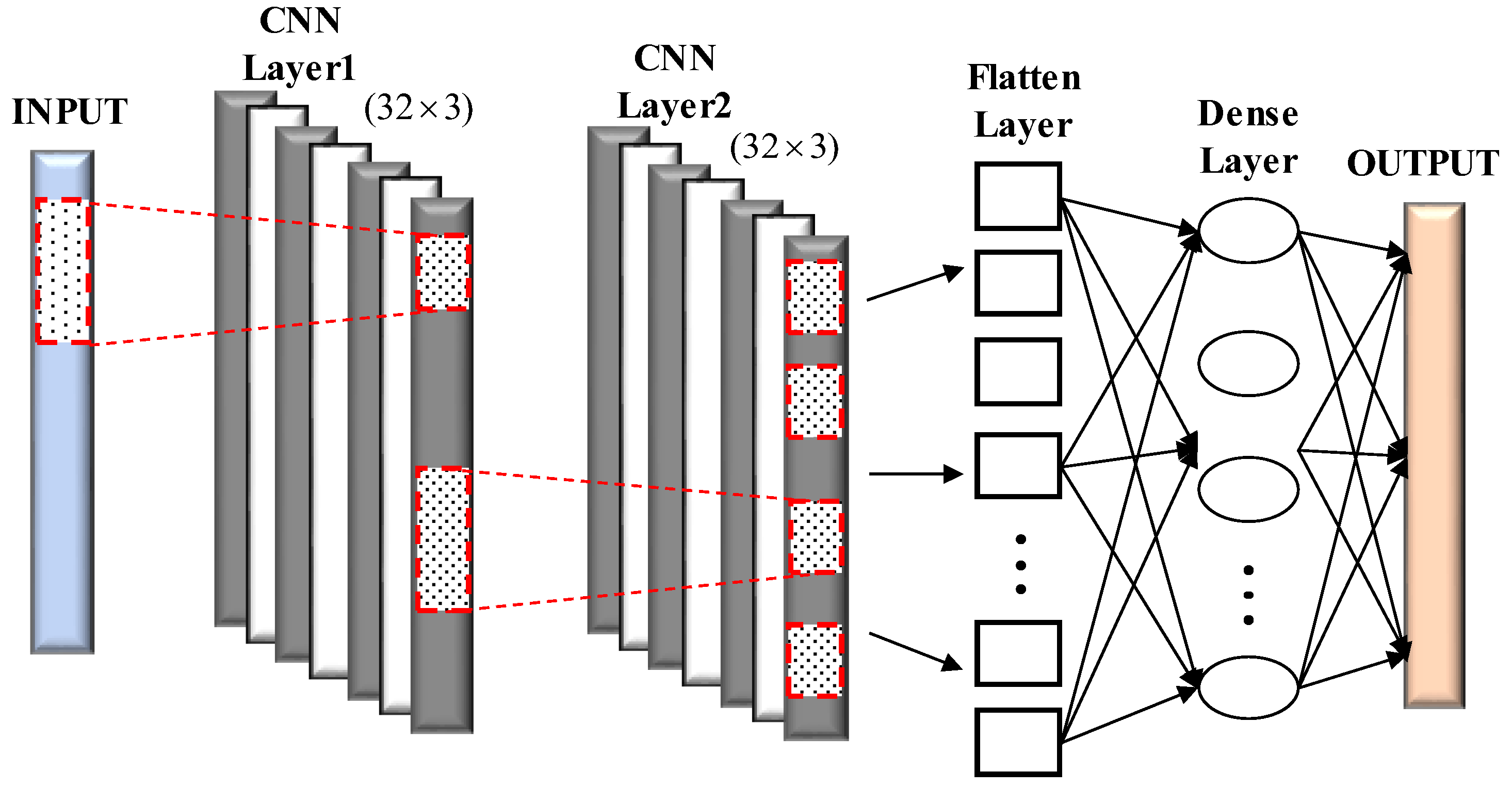
2.3. Convolutional Neural Network

In this paper, we use the most general convolutional neural network as an example to verify the effectiveness of the proposed method. CNNs are developed and inspired by the structure of the visual system and are centered on extracting features from the input data using filters. The deeper the network depth, the deeper the level of features extracted from the input data. From its beginning to now, 1D, 2D and 3D CNNs have been developed. The tasks processed by different methods are usually different. For example, 1D CNN is suitable for processing sequence data, while 2D and 3D CNNs are usually applied to problems such as images, videos and texts [32]. Since the seismic impedance inversion is a multi-sequence input problem and contains coupling between different curves, the convolution of the CNN network used in this study is 1D structures.
Figure 3 shows the detailed architecture of the convolutional neural network used in this paper to facilitate the reader to reproduce the results of the subsequent numerical experiments. The multi-scale data acquired in the previous section is used as input for feature extraction by the convolutional neural network. CNNs can be used for local features processing as they take into account the correlation of local input data. The framework used here consists of two convolutional layers, which have the same parameters ( 32 , 3 × 1 , 1 ) . ReLu activation functions [33] are connected after each convolutional layer to accomplish the nonlinear task. In addition, a dropout layer is added after the second convolutional layer to prevent the network from overfitting. After going through the convolutional neural network for feature extraction, the extracted features are flattened and then fed into the fully connected layer. Finally, the output of the fully connected layer is given to the final output layer to obtain the final prediction of the network. We utilize the mean square error to measure the loss between the network outputs and the given labels, and then the Adam optimizer [34] is adopted to optimize the network parameters (i.e., weights and biases) to obtain a deep neural network that can perform seismic impedance inversion. In this paper, we obtain the relatively optimal network parameters, including the number of layers, the number of neurons per layer and the size of the convolutional kernel, etc., through iterative experiments. This relies heavily on the experimenter’s experience, and it might be good to combine the choice of network parameters with an optimization algorithm.

2.4. Transfer Learning Strategy

Based on the above theory and strategy, we can obtain satisfactory results when the training dataset is sufficient (e.g., synthetic model data). However, in practice, it is difficult, if not impossible, to have sufficient training datasets (i.e., well-logs data) to be used directly for network training. Transfer learning is a research problem in machine learning that focuses on using the knowledge gained in solving one problem and applying it to another different but related problem for the purpose of accomplishing the task of a different problem [35]. The physical system (i.e., seismic forward modeling) used for the synthesized model data is an approximate representation of the actual problem, which is consistent with the conditions applied for transfer learning. Therefore, we introduce the transfer learning strategy for practical data applications to alleviate the problem that data-driven methods cannot achieve good application performance due to the limited amount of training data. The closer the simulated data is to the actual data, the more reliable the pre-trained network will be. In this paper, we first pre-train the network with synthetic model data to obtain a robust network and use the synthetic data for testing and validation. Then, the layers other than the fully connected layers in the pre-trained network are fixed [36] and the network parameters of the non-fixed layers are fine-tuned using the well-logs data so that the updated network is applicable to the actual data. In this way, the proposed method can be easily extended to practice case to obtain reliable seismic impedance.

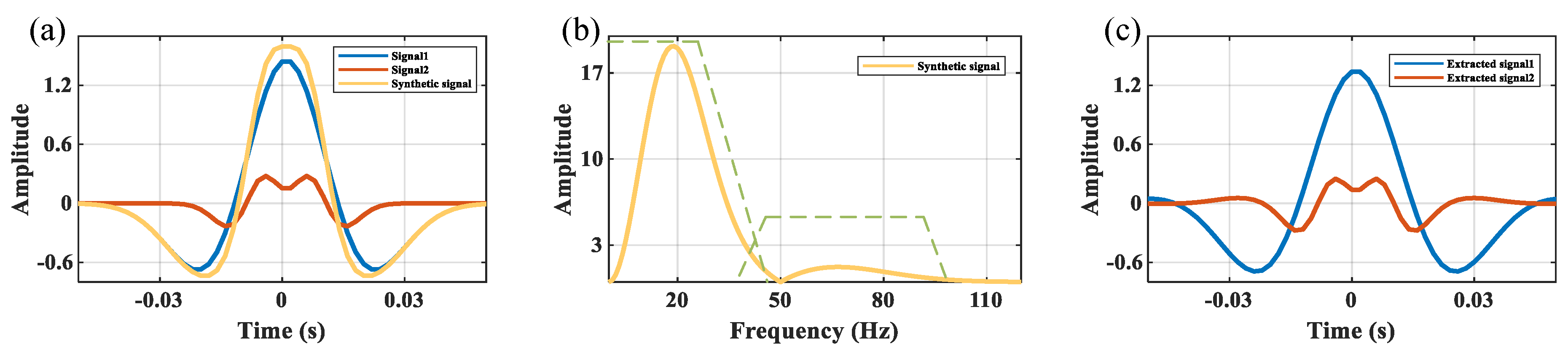
2.5. f-x Filtering Technique
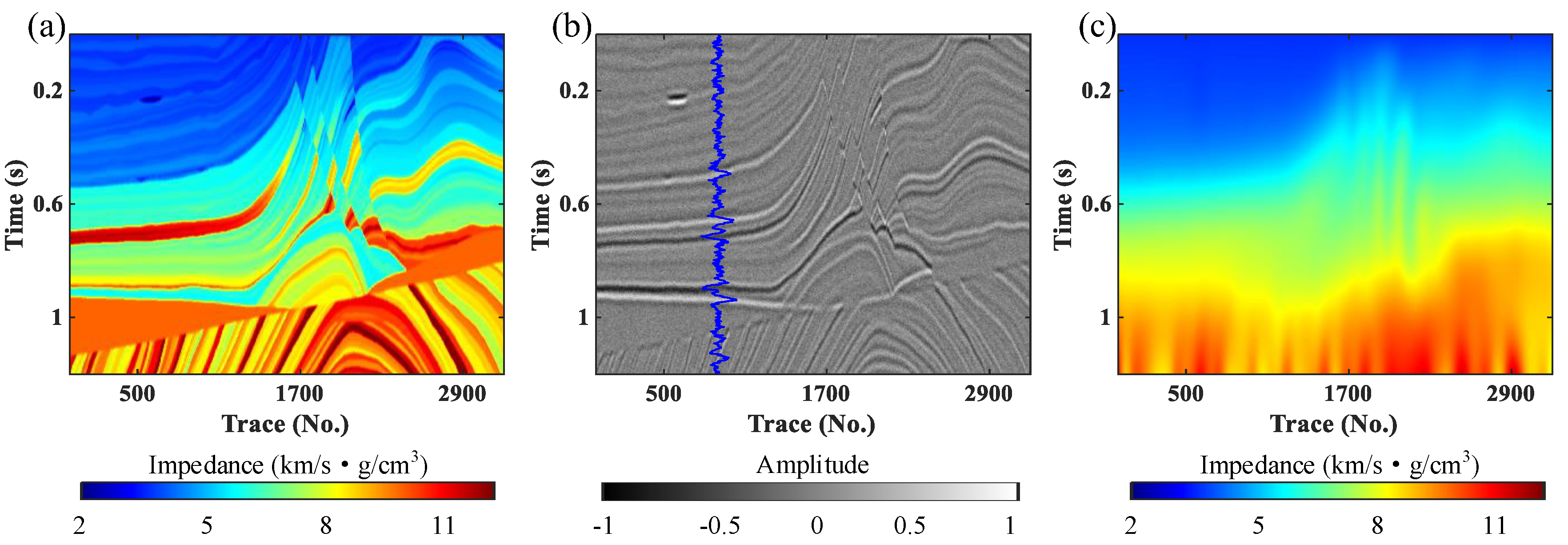
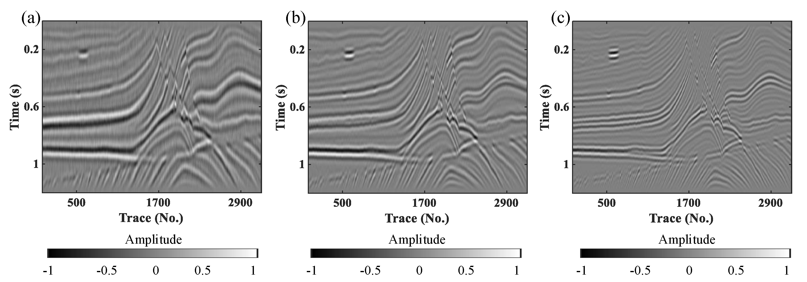
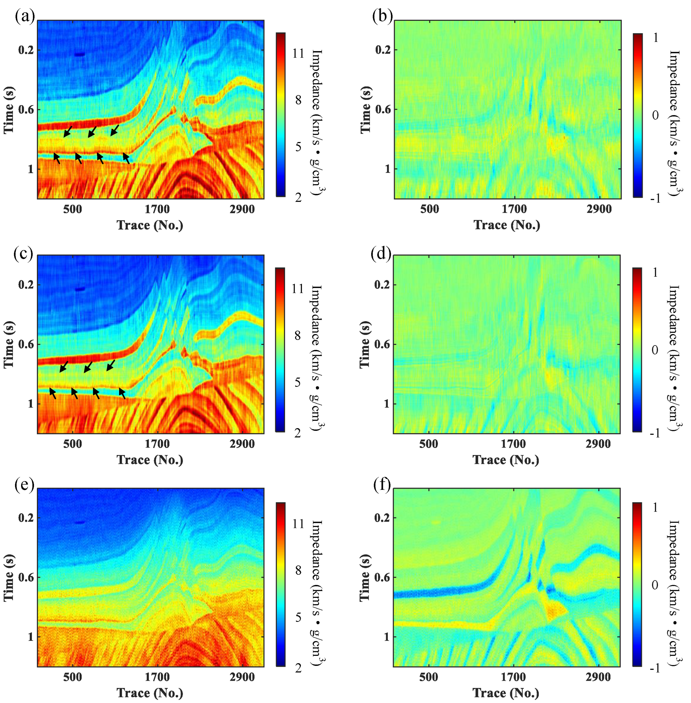
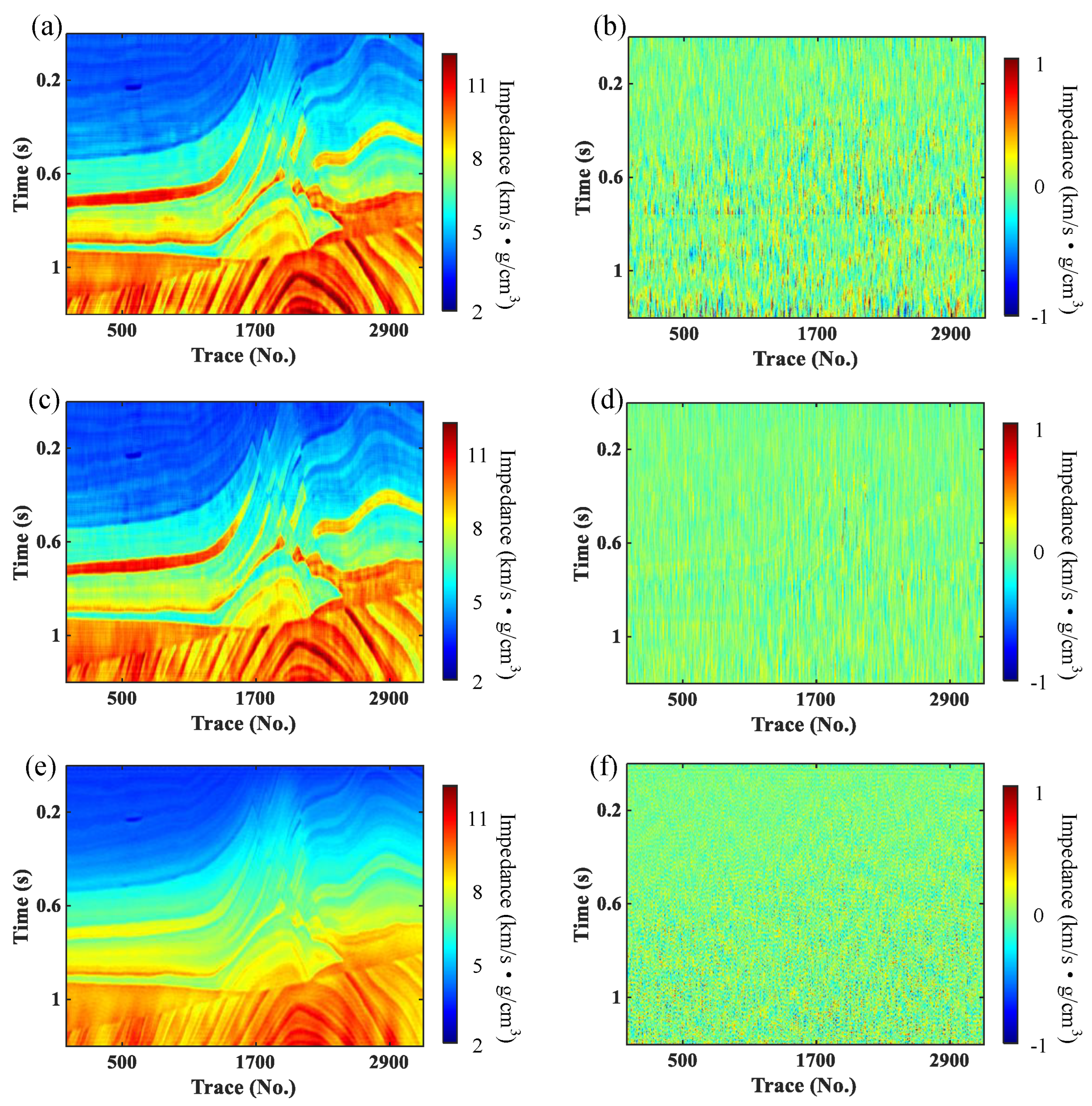
Since the proposed method performs seismic impedance inversion trace-by-trace, we further introduce the f-x prediction filtering technique to improve the lateral continuity of the inversion results, based on the assumption that the signal can be represented as a superposition of events with linear time differences. For a linear event, the signal in the trace n at any temporal frequency f can be expressed by: [37]
S n ( f ) = S n 1 ( f ) e i 2 π f ϑ Δ x
where S n ( f ) represent Fourier transform of the n t h trace of the original signal S n ( t ) , ϑ and Δ x represent apparent slowness and spatial interval of adjacent trace, respectively, and i = 1 . If p linear times are superimposed in the t-x domain, the following equation can be obtained:
S n ( f ) = a 1 S n 1 ( f ) + a 2 S n 2 ( f ) + + a p S n p ( f )
Equation (4) can be written in the form of a prediction error as follows:
k = 0 p g k S n k ( f ) = 0
where g k represents the coefficients of prediction error filter and g 0 = 1 . The filtering operator g k is obtained by solving Equation (5), which can then be applied to the spatial trace to obtain the filtered results for frequency f. Once all frequencies have been filtered, inverse Fourier transform is performed to obtain the filtered t-x domain data.

3. Results

To verify the effectiveness of the proposed method, we apply the method to a benchmark Marmousi model and an actual data set, respectively. The seismic impedance inversion results of the multi-scale strategy are compared with those using conventional seismic data as input and those based on the model-driven method. For the validity and fairness of the result comparison, the deep neural networks used in the different methods are identical in the numerical experiments. In the subsequent experiments, the proposed method in this paper is called multi-scale seismic impedance inversion (MSII) and the conventional method is called single-scale seismic impedance inversion (SSII). The model-driven impedance inversion method is denoted MDII. In addition, to quantitatively evaluate the goodness of the inversion results, the root mean square error (RMSE) is introduced as a criterion to evaluate them with the following expression:
RMSE = 1 n i = 1 n ( y i Y i ˜ ) 2
where y i and Y i ˜ denote reference values and predicted values, respectively. n indicates the total number of data points.

3.1. Synthetic Data Test

The validity of the proposed method is first tested on a benchmark Marmousi model. The model contains 3201 traces and 600 time samples with a time interval of 2 ms, as shown in Figure 4a. Then, synthetic seismic records can be obtained using the forward modeling method described in the theoretical section. Figure 4b shows the seismogram with a signal-to-noise ratio of two, which will be used in subsequent tests to verify the performance of the method. The seismic wavelet used here is a 20 Hz zero-phase Ricker wavelet. The initial model of low-frequency impedance obtained from the true impedance model using the low-pass filtering method is shown in Figure 4c. Figure 5 shows the multi-scale seismic data extracted using the multi-scale strategy. We randomly select 50 traces from the true impedance models to construct the training dataset, and 15% of this training dataset is used as the validation set. The network is pre-trained using the constructed training dataset, and then the pre-trained network is used in the 2D Marmousi model to implement the seismic impedance inversion of the entire profile.
Figure 6a,c,e shows the inversion results of SSII, MSII and MDII without f-x filtering, respectively. It can be seen that the inversion results of data-driven methods (i.e., SSII and MSII) outperform those of model-driven methods (i.e., MDII). The inversion results of MSII are more stable and have better continuity compared to the inversion results of SSII. Moreover, in some localized regions (black arrows), the inversion results of MSII reveal more details than those of SSII and are more consistent with the reference model. Figure 6b,d,f shows the normalized residuals between the inversion results of SSII, MSII and MDII and the true values. It can be seen that the residuals of the inversion results of data-driven methods are smaller compared to those of model-driven methods. The residuals of the inversion results of the data-driven methods are concentrated around the value of 0, which indicates the effectiveness of the methods, but the residuals of the MSII-based inversion results are smaller compared to the residuals of the SSII-based inversion results. However, since these methods perform impedance inversion trace-by-trace, their inversion results have poor lateral continuity, which increases the difficulty of subsequent interpretation. For this reason, we further introduce the f-x filtering technique to improve the continuity of the inversion results. Figure 7a,c,e show the inversion results of SSII, MSII and MDII with f-x filtering, respectively. It shows that the inversion results with f-x filtering can effectively improve the lateral stability. The normalized residual profiles (Figure 7b,d,f) of inversion results without and with f-x filtering show that the filtering process does not damage the effective signal and also show the better stability of MSII compared to SSII and MDII. In addition, the validity of the proposed method is verified quantitatively by comparing the RMSEs recorded in Table 1.

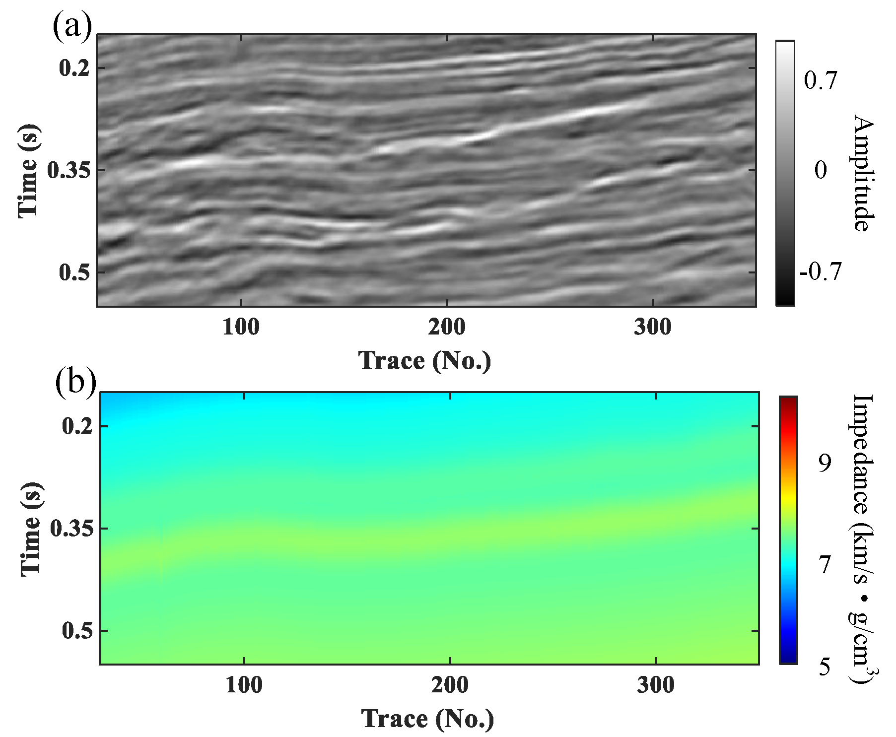
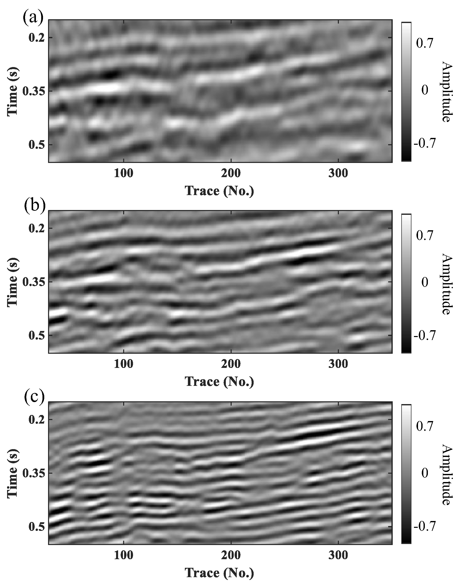
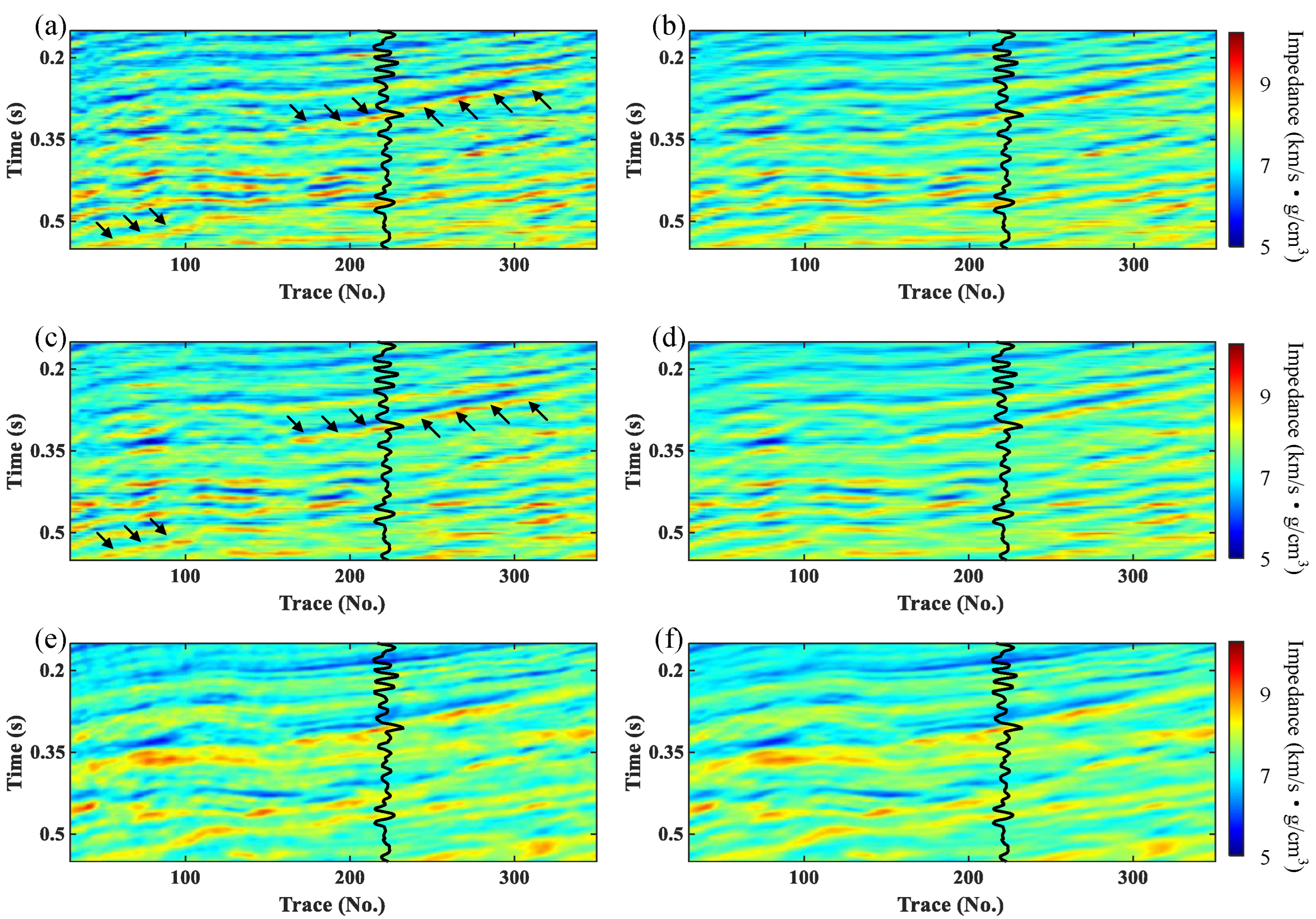
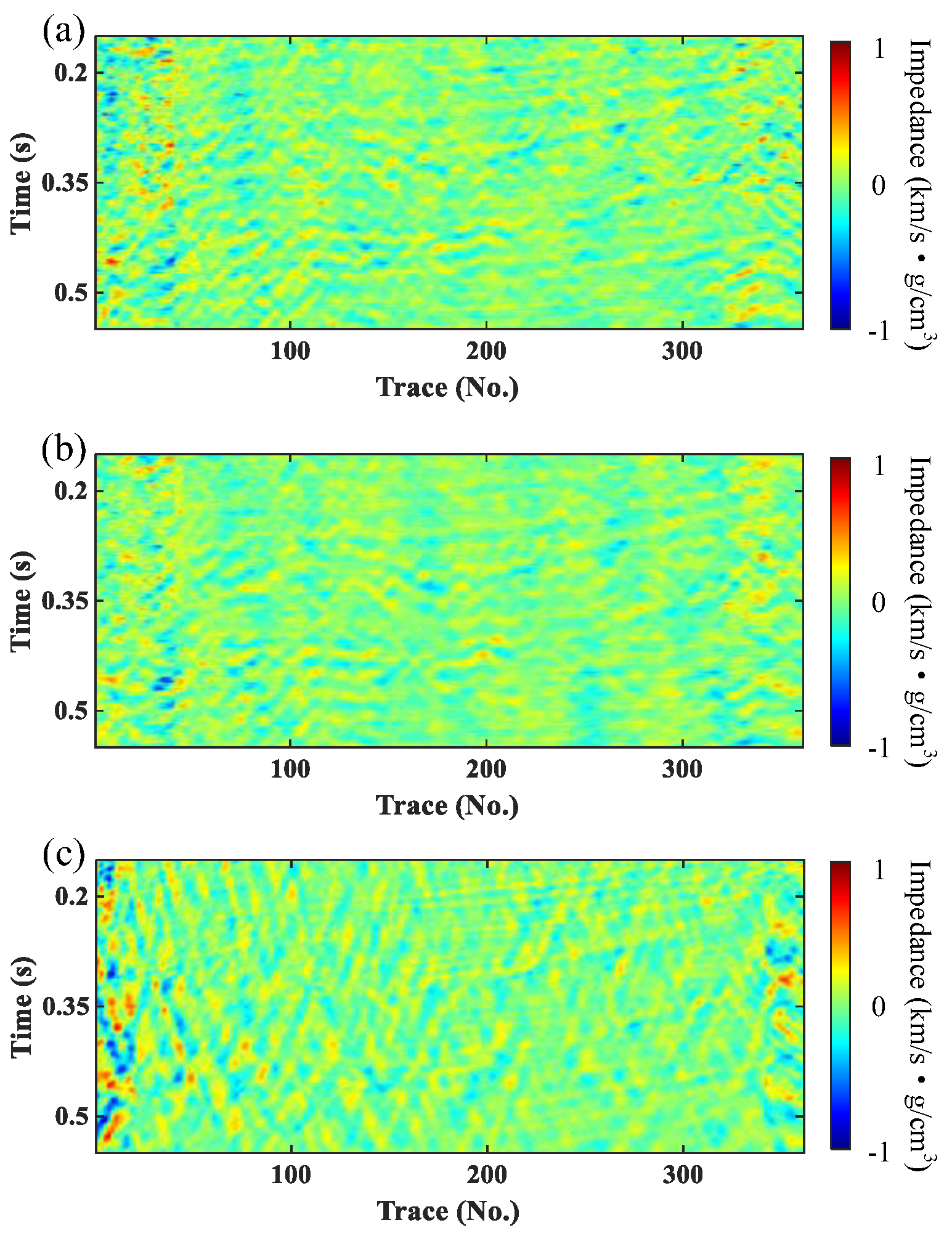
3.2. Field Data Example

Based on the success of the MSII method on synthetic model data, we further apply it to real data to confirm the applicability of the proposed method to real problems. A small 2D actual seismic data is used to test the effectiveness of the method, as shown in Figure 8a. In addition to the seismic traces, the data set contains data from four wells. The initial model of low-frequency impedance obtained based on the known well-logs data and the horizon information picked up from the seismic data is shown in Figure 8b. Figure 9 shows the multi-scale seismic data extracted using the multi-scale strategy. We select three of the four well-logs data to construct the training dataset, while the other well-log data is used as a blind well to validate the inversion results. Due to the limited well-logs data, it is difficult to obtain a robust network by using them directly for network training. We introduce the transfer learning strategy to overcome this problem. First, the layers of the network pre-trained using model data are fixed except for the fully connected layer. We then fine-tune the network pre-trained from the model data using the training dataset constructed from the well-logs data to ensure the stability of the network and make the updated network applicable to the actual data. Multi-scale data including multi-scale seismic data and low-frequency initial models are used as network inputs to finally realize seismic impedance inversion and obtain 2D seismic impedance profiles.
Figure 10a–e show the inversion results of SSII, MSII and MDII without and with f-x filtering, respectively. Blind well-log curves are also projected on the inversion results at the same time to facilitate comparison. The inversion results from all three methods can be well matched to the well-log curves at the blind well location. The data-driven approach yields higher resolution inversion results than the model-driven approach. In addition, the MSII results reveal more details and have better lateral continuity (black arrows) than the those of SSII. The continuity of the inversion results of SSII, MSII and MDII is further improved by the f-x filtering technique, as shown in Figure 10b,d,f. The normalized residual profiles (Figure 11a–c) of inversion results without and with f-x filtering show that the filtering process does not damage the effective signal. It also indicates that MSII has better stability compared to SSII and MDII. These findings are consistent with the conclusions of the synthetic model numerical experiments, which further validates the validity and applicability of the proposed method. Table 2 lists the RMSE between the blind well-log and the inversion results of SSII, MSII and MDII without and with f-x filtering. It is clear that the RMSE of inverted impedance from MSII with f-x filtering is the smallest. In summary, a series of numerical tests show that MSII has the best performance.

4. Conclusions

We developed a data-driven seismic impedance inversion method based on multi-scale strategy, which improves the resolution and stability of the inversion results of the data-driven method. The proposed method (MSII) is first applied to model data for impedance inversion and the inversion results are compared with those based on SSII and MDII. It is shown that the inversion results based on the data-driven approach (i.e., SSII and MSII) outperform the inversion results based on the model-driven approach (i.e., MDII), while MSII is optimal. In addition, we introduced the f-x filtering technique to improve the continuity of the inversion results and thus obtain a more geologically reliable impedance profile. Then, the transfer learning algorithm was introduced to overcome the limitation of limited training dataset in real data, thus successfully applying the proposed method to real data with satisfactory results. Overall, both synthetic model testing and practical data application qualitatively and quantitatively validate the effectiveness of the proposed method. However, the proposed approach is still fully data-driven and still relies heavily on the training dataset, although the transfer learning strategy alleviates the problem to some extent. Our next work will aim to establish a closed-loop data-driven framework for label-free MSII by introducing a known physical system, and to capture the uncertainty of the inversion results to achieve reliability evaluation of the inversion results.

Author Contributions

G.Z.: Conceptualization, methodology, code, writing—original draft preparation; X.C.: Supervision, software; J.L.: Validation, investigation; K.G.: Writing—Reviewing and editing. All authors have read and agreed to the published version of the manuscript.

Funding

Please add: This work was financially supported by the National Natural Science Foundation of China under Grant 41774131 and 41774129, supported in part by the National Key Research and Development Program of China under Grant 2019YFC0312000, supported in part by R&D Department of China National Petroleum Corporation (Investigations on fundamental experiments and advanced theoretical methods in geophysical prospecting applications) under Grant 2022DQ0604-04.

Data Availability Statement

The original contributions presented in the study are included in the article; further inquiries can be directed to the corresponding author.

Acknowledgments

We would like to thank the State Key Laboratory of Petroleum Resources and Prospecting, and National Engineering Laboratory for Offshore Oil Exploration for supporting this work.

Conflicts of Interest

The authors declare that the research was conducted in the absence of any commercial or financial relationships that could be construed as a potential conflict of interest.

References

  1. Hamid, H.; Pidlisecky, A. Multitrace impedance inversion with lateral constraints. Geophysics 2015, 80, M101–M111. [Google Scholar] [CrossRef]
  2. Zhang, J.; Li, J.; Chen, X.; Li, Y. Geological structure-guided hybrid MCMC and Bayesian linearized inversion methodology. J. Pet. Sci. Eng. 2021, 199, 108296. [Google Scholar] [CrossRef]
  3. Wang, N.; Xing, G.; Zhu, T.; Zhou, H.; Shi, Y. Propagating Seismic Waves in VTI Attenuating Media Using Fractional Viscoelastic Wave Equation. J. Geophys. Res. Solid Earth 2022, 127, e2021JB023280. [Google Scholar] [CrossRef]
  4. Farfour, M.; Yoon, W.J.; Kim, J. Seismic attributes and acoustic impedance inversion in interpretation of complex hydrocarbon reservoirs. J. Appl. Geophys. 2015, 114, 68–80. [Google Scholar] [CrossRef]
  5. Kemper, M.; Gunning, J. Joint impedance and facies inversion–seismic inversion redefined. First Break 2014, 32, 89–95. [Google Scholar] [CrossRef]
  6. Li, K.; Yin, X.; Liu, J.; Zong, Z. An improved stochastic inversion for joint estimation of seismic impedance and lithofacies. J. Geophys. Eng. 2019, 16, 62–76. [Google Scholar] [CrossRef] [Green Version]
  7. Madiba, G.B.; McMechan, G.A. Seismic impedance inversion and interpretation of a gas carbonate reservoir in the Alberta Foothills, western Canada. Geophysics 2003, 68, 1460–1469. [Google Scholar] [CrossRef]
  8. Riedel, M.; Bellefleur, G.; Mair, S.; Brent, T.A.; Dallimore, S.R. Acoustic impedance inversion and seismic reflection continuity analysis for delineating gas hydrate resources near the Mallik research sites, Mackenzie Delta, Northwest Territories, Canada. Geophysics 2009, 74, B125–B137. [Google Scholar] [CrossRef]
  9. She, B.; Wang, Y.; Liu, Z.; Cai, H.; Liu, W.; Hu, G. Seismic impedance inversion using dictionary learning-based sparse representation and nonlocal similarity. Interpretation 2019, 7, SE51–SE67. [Google Scholar] [CrossRef]
  10. Zhou, L.; Liu, X.; Li, J.; Liao, J. Robust AVO inversion for the fluid factor and shear modulus. Geophysics 2021, 86, R471–R483. [Google Scholar] [CrossRef]
  11. Zhou, L.; Li, J.; Yuan, C.; Liao, J.; Chen, X.; Liu, Y.; Pan, S. Bayesian Deterministic Inversion Based on the Exact Reflection Coefficients Equations of Transversely Isotropic Media With a Vertical Symmetry Axis. IEEE Trans. Geosci. Remote Sens. 2022, 60, 5915715. [Google Scholar] [CrossRef]
  12. Traore, B.B.; Kamsu-Foguem, B.; Tangara, F. Deep convolution neural network for image recognition. Ecol. Inform. 2018, 48, 257–268. [Google Scholar] [CrossRef] [Green Version]
  13. Hu, B.; Lu, Z.; Li, H.; Chen, Q. Convolutional neural network architectures for matching natural language sentences. Adv. Neural Inf. Process. Syst. 2014, 27, 1–9. [Google Scholar]
  14. Khan, S.; Rahmani, H.; Shah, S.A.A.; Bennamoun, M. A Guide to Convolutional Neural Networks for Computer Vision. In Synthesis Lectures on Computer Vision; Springer Nature: Cham, Switzerland, 2018; Volume 8, pp. 1–207. [Google Scholar]
  15. Zhang, G.; Wang, Z.; Chen, Y. Deep learning for seismic lithology prediction. Geophys. J. Int. 2018, 215, 1368–1387. [Google Scholar] [CrossRef]
  16. Zhang, J.; Li, J.; Chen, X.; Li, Y.; Tang, W. A spatially coupled data-driven approach for lithology/fluid prediction. IEEE Trans. Geosci. Remote Sens. 2020, 59, 5526–5534. [Google Scholar] [CrossRef]
  17. Wu, X.; Shi, Y.; Fomel, S.; Liang, L.; Zhang, Q.; Yusifov, A. FaultNet3D: Predicting Fault Probabilities, Strikes, and Dips With a Single Convolutional Neural Network. IEEE Trans. Geosci. Remote Sens. 2019, 57, 9138–9155. [Google Scholar] [CrossRef]
  18. Bi, Z.; Wu, X.; Geng, Z.; Li, H. Deep Relative Geologic Time: A Deep Learning Method for Simultaneously Interpreting 3-D Seismic Horizons and Faults. J. Geophys. Res. Solid Earth 2021, 126, e2021JB021882. [Google Scholar] [CrossRef]
  19. Saad, O.M.; Chen, Y. A fully unsupervised and highly generalized deep learning approach for random noise suppression. Geophys. Prospect. 2021, 69, 709–726. [Google Scholar] [CrossRef]
  20. Kaur, H.; Pham, N.; Fomel, S. Seismic data interpolation using deep learning with generative adversarial networks. Geophys. Prospect. 2021, 69, 307–326. [Google Scholar] [CrossRef]
  21. Das, V.; Pollack, A.; Wollner, U.; Mukerji, T. Convolutional neural network for seismic impedance inversionCNN for seismic impedance inversion. Geophysics 2019, 84, R869–R880. [Google Scholar] [CrossRef]
  22. Li, S.; Liu, B.; Ren, Y.; Chen, Y.; Yang, S.; Wang, Y.; Jiang, P. Deep-learning inversion of seismic data. arXiv 2019, arXiv:1901.07733. [Google Scholar] [CrossRef]
  23. Puzyrev, V.; Egorov, A.; Pirogova, A.; Elders, C.; Otto, C. Seismic inversion with deep neural networks: A feasibility analysis. In Proceedings of the 81st EAGE Conference and Exhibition 2019, London, UK, 3–6 June 2019; pp. 1–5. [Google Scholar]
  24. Zhang, J.; Li, J.; Chen, X.; Li, Y.; Huang, G.; Chen, Y. Robust deep learning seismic inversion with a priori initial model constraint. Geophys. J. Int. 2021, 225, 2001–2019. [Google Scholar] [CrossRef]
  25. Kazei, V.; Ovcharenko, O.; Plotnitskii, P.; Peter, D.; Zhang, X.; Alkhalifah, T. Mapping full seismic waveforms to vertical velocity profiles by deep learning. Geophysics 2021, 86, R711–R721. [Google Scholar] [CrossRef]
  26. Cao, D.; Su, Y.; Cui, R. Multi-parameter pre-stack seismic inversion based on deep learning with sparse reflection coefficient constraints. J. Pet. Sci. Eng. 2022, 209, 109836. [Google Scholar] [CrossRef]
  27. Zhang, J.; Sun, H.; Zhang, G.; Zhao, X. Deep Learning Seismic Inversion Based on Prestack Waveform Datasets. IEEE Trans. Geosci. Remote Sens. 2022, 60, 4511311. [Google Scholar] [CrossRef]
  28. Boonyasiriwat, C.; Valasek, P.; Routh, P.; Cao, W.; Schuster, G.T.; Macy, B. An efficient multiscale method for time-domain waveform tomography. Geophysics 2009, 74, WCC59–WCC68. [Google Scholar] [CrossRef] [Green Version]
  29. Bunks, C.; Saleck, F.M.; Zaleski, S.; Chavent, G. Multiscale seismic waveform inversion. Geophysics 1995, 60, 1457–1473. [Google Scholar] [CrossRef]
  30. Pan, X.; Li, L.; Zhang, G. Multiscale frequency-domain seismic inversion for fracture weakness. J. Pet. Sci. Eng. 2020, 195, 107845. [Google Scholar] [CrossRef]
  31. Ren, Z.; Liu, Y.; Zhang, Q. Multiscale viscoacoustic waveform inversion with the second generation wavelet transform and adaptive time–space domain finite-difference method. Geophys. J. Int. 2014, 197, 948–974. [Google Scholar] [CrossRef] [Green Version]
  32. Li, Z.; Liu, F.; Yang, W.; Peng, S.; Zhou, J. A survey of convolutional neural networks: Analysis, applications, and prospects. IEEE Trans. Neural Netw. Learn. Syst. 2021, in press. [Google Scholar] [CrossRef]
  33. Ramachandran, P.; Zoph, B.; Le, Q.V. Searching for activation functions. arXiv 2017, arXiv:.05941. [Google Scholar]
  34. Sun, S.; Cao, Z.; Zhu, H.; Zhao, J. A survey of optimization methods from a machine learning perspective. IEEE Trans. Cybern. 2019, 50, 3668–3681. [Google Scholar] [CrossRef] [PubMed]
  35. Pan, S.J.; Yang, Q. A survey on transfer learning. IEEE Trans. Knowl. Data Eng. 2009, 22, 1345–1359. [Google Scholar] [CrossRef]
  36. Zhang, C.-L.; Luo, J.-H.; Wei, X.-S.; Wu, J. In defense of fully connected layers in visual representation transfer. In Proceedings of the Pacific Rim Conference on Multimedia, Harbin, China, 28–29 September 2017; pp. 807–817. [Google Scholar]
  37. Chen, K.; Sacchi, M.D. Making Fx Projection Filters Robust to Erratic Noise. In SEG Technical Program Expanded Abstracts 2014; Society of Exploration Geophysicists: Houston, TX, USA, 2014; pp. 4371–4375. [Google Scholar]
Figure 1. Schematic diagram of multi-scale seismic data extraction. (a) Synthesized seismic signal. (b) The amplitude spectrum of the synthesized signal, where the dashed green line indicates the crossover window. (c) The extracted multi-scale seismic data.
Remotesensing 14 06056 g001
Figure 2. Deep learning seismic impedance inversion framework based on multi-scale strategy.
Remotesensing 14 06056 g002
Figure 3. Network structure diagram of CNN-based seismic inversion.
Remotesensing 14 06056 g003
Figure 4. Synthetic data test of Marmousi model: (a) True impedance model. (b) Synthetic seismic records. (c) Initial impedance model.
Remotesensing 14 06056 g004
Figure 5. Multi-scale seismic data: (a) Low frequency data. (b) Medium frequency data. (c) High frequency data.
Remotesensing 14 06056 g005
Figure 6. (a) The inverted impedance using SSII without f-x filtering. (b) The residual profiles between SSII inversion results without f-x filtering and reference values. (c) The inverted impedance using MSII without f-x filtering. (d) The residual profiles between MSII inversion results without f-x filtering and reference values. (e) The inverted impedance using MDII without f-x filtering. (f) The residual profiles between MDII inversion results without f-x filtering and reference values.
Remotesensing 14 06056 g006
Figure 7. (a) The inverted impedance using SSII with f-x filtering. (b) The residual profiles of SSII inversion results without and with f-x filtering. (c) The inverted impedance using MSII with f-x filtering. (d) The residual profiles of MSII inversion results without and with f-x filtering. (e) The inverted impedance using MDII with f-x filtering. (f) The residual profiles of MDII inversion results without and with f-x filtering.
Remotesensing 14 06056 g007
Figure 8. Real data test: (a) Original seismic records. (b) Initial impedance model.
Remotesensing 14 06056 g008
Figure 9. Multi-scale seismic data: (a) Low frequency data. (b) Medium frequency data. (c) High frequency data.
Remotesensing 14 06056 g009
Figure 10. (a) The inverted impedance using SSII without f-x filtering. (b) The inverted impedance using SSII with f-x filtering. (c) The inverted impedance using MSII without f-x filtering. (d) The inverted impedance using MSII with f-x filtering. (e) The inverted impedance using MDII without f-x filtering. (f) The inverted impedance using MDII with f-x filtering.
Remotesensing 14 06056 g010
Figure 11. (a) The residual profiles of SSII inversion results without and with f-x filtering. (b) The residual profiles of MSII inversion results without and with f-x filtering. (c) The residual profiles of MDII inversion results without and with f-x filtering.
Remotesensing 14 06056 g011
Table 1. The RMSE of the inversion results (Marmousi model) of SSII, MSII and MDII combined with and without f-x filtering.
Without f-x FilteringWith f-x Filtering
SSII0.590.50
MSII0.480.44
MDII0.900.85
Table 2. The RMSE of the inversion results (blind well) of SSII, MSII and MDII combined with and without f-x filtering.
Without f-x FilteringWith f-x Filtering
SSII1.411.25
MSII1.271.22
MDII1.511.40
Publisher’s Note: MDPI stays neutral with regard to jurisdictional claims in published maps and institutional affiliations.

