Article

Evaluation of Mangrove Wetlands Protection Patterns in the Guangdong–Hong Kong–Macao Greater Bay Area Using Time-Series Landsat Imageries

1
School of Geography, South China Normal University, Guangzhou 510631, China
2
Key Laboratory of Natural Resources Monitoring in Tropical and Subtropical Area of South China, Ministry of Natural Resources, Guangzhou 510631, China
3
School of Computer Science, South China Normal University, Guangzhou 510631, China
4
School of Geography, Nanjing Normal University, Nanjing 210023, China
5
Institute of Space and Earth Information Science, Fok Ying Tung Remote Sensing Science Building, The Chinese University of Hong Kong, Shatin, Hong Kong, China
*
Author to whom correspondence should be addressed.
Remote Sens. 2022, 14(23), 6026; https://doi.org/10.3390/rs14236026
Submission received: 8 October 2022 / Revised: 14 November 2022 / Accepted: 25 November 2022 / Published: 28 November 2022

Abstract

:
The protection of mangroves through nature reserves has been demonstrated to be effective. There were many studies evaluating the mangrove protection effect. However, the evaluation of mangrove growth quality with positive or negative growth trends, as well as restoration potential against disturbance in nature reserves, is still lacking. Thus, this study proposed a hierarchical evaluation framework for mangrove protection in nature reserves, which takes long-term metrics at three levels of loss and gain areas, patch pattern dynamics, and pixel growth trends into account. The continuous change detection and classification (CCDC) was utilized to identify the change condition of mangroves in six nature reserves of the Guangdong–Hong Kong–Macao Greater Bay Area. The Entropy Weight Technique for Order Preference by Similarity to Ideal Solution (TOPSIS) was utilized for scores evaluation of protection effort comparison from 2000 to 2020. The study results had the following three main findings. Firstly, the mangrove forest area increased by about 294.66 ha in four reserves and slightly decreased by about 58.86 ha in two. Most reserves showed an improved patches intact pattern and more positive growth trends. Secondly, the establishment of nature reserves and afforestation were the main causes of mangrove area gain. Until 2010, aquaculture, agriculture, and urban development were the biggest threats to mangroves. Finally, the protection of the reserves was successful in the early decades, but the general evaluation scores showed a decline in recent years once we considered the growth trends for quality. The proposed hierarchical evaluation methods provide a new sight to research the impacts of abrupt change and protection resilience status of the gradual restoration of nature reserves.

1. Introduction

Mangroves are dynamic ecosystems found in tropical and subtropical coastal intertidal zones. They are essential for preserving the shoreline, biodiversity, and essential ecosystem services [1,2]. They also help lessen the devasting effects of natural disasters such as hurricanes and tsunamis. However, mangrove distribution and habitat quality change quickly due to human activities [3,4,5] and the majority of mangrove loss (62%) around the world has been a result of human impact along the coast since the start of the 21st century [3]. In two decades, China’s mangrove area fell by over 50% [6]. Anthropogenic disturbance is the primary cause of mangrove loss in Asia, accounting for 75% of total loss [4]. Mangrove destruction is typically caused by inappropriate rapid urbanization [3,4,6], the expansion of aquaculture and agriculture [7], pollution, and overextraction [5].
A key step in alleviating the negative effects of human activity on mangrove forests is the establishment of nature reserves [8] which were proven to be more effective [9,10,11]. The Ramsar Convention, which was formed in 1971 [12], indicates that it should establish reserves to promote wetlands and waterfowl conservation. Accordingly, deforestation rates of mangroves have declined in the past decade [5] and mangrove losses caused by direct human intervention have declined by 73% [3]. Therefore, China has taken a variety of measures to preserve and rehabilitate mangroves, including establishing nature reserves and introducing the national key ecological and financial improvement plan [13]. Without the intensive deforestation and occupation of mangroves, we wonder whether traditional evaluation metrics, such as area loss, are reliable and effective for nature reserve evaluation [14].
Recently, increasingly more studies have begun to quantify the effects of conservation [15], using mangrove-evaluation metrics such as habitat cover and biodiversity [11], connectivity and fragmentation [16], and even geographical distribution [17], as well as the causes of loss [3]. Temporally, the area and landscape of forests, as well as their dynamic changes [18,19,20,21,22], are the most commonly used indicators in the effectiveness analysis of forests in nature reserves. In other words, most studies have concentrated on assessing a specific moment or interval. However, existing research has confirmed that mangroves’ resistance to disasters [23,24] and the biodiversity [11] of coastal ecosystems are related to growth quality. To detect the growth status, such as degradation and recovery of mangroves that have been protected, gradual change detection needs long-term mission data. Although the area and landscape dynamics have been used to assess the conservation effect of mangrove nature reserves [18], few studies have identified the growth quality and trends for mangrove resilience in nature reserves.
Monitoring the obvious loss and restoration of mangroves is easily accomplished and shows what happened, while the growth trends of individual mangroves in a nature reserve can help predict what will be. Today, optical sensors, such as those used in the Landsat missions, have the unique advantage of providing seamless global long-term observations that radar or lidar sensors cannot. Methods that use dense Landsat Time Series (LTS) have shown an enhanced capability for recording vegetation phenology and various kinds of inter-annual land [25,26,27]. The utilization of dense LTS not only fills spatial and temporal data gaps in cloudy regions [28,29] but can also track growth trends, including in wild forests and urban green spaces [25,30]. However, as we all know, wetlands are one of the most difficult land cover classifications to map using satellite data [31], particularly mangroves with coastal tidal wetlands that are highly dynamic in terms of water level from tide and sea level changes [32,33]. As a result, there is uncertainty existing when using LTS data to map mangrove classification and it is imperative to develop novel methods and evaluation strategies that integrate the trajectories of mangrove disturbance and recovery for the accurate mapping of the growth trends.
In this study, the continuous change detection and classification (CCDC) method [34] was employed to track the loss–restoration of mangroves with both positive (increasing) and negative (decreasing) trends. CCDC employs a per-pixel fitting method to capture seasonal dynamics of land cover as well as trends in inter-year greening and browning, included in the urban area and carbon dynamics [25,35]. One advantage of model fitting is that it lessens reliance on individual observations and can reduce the requirement for a full cloudless image, which is particularly helpful for monitoring mangrove ecosystems [36,37,38,39]. Mangrove growth trends without changes depend on the long-term trend to describe the slope changes before and after the restoration.
The mangroves in the GBA are distributed widely, and nature reserves in the GBA are typical in the north of the world’s mangrove distribution area. The GBA has experienced a population and economic boost since the 1980s with a significant amount of land reclamation [1]. Despite the existence of numerous nature reserves, protecting mangroves is a great challenge due to intensive human disturbance in their early decades, such as reclamation and landfills [1,5], and the protective effects of recent ecological restoration are frequently unknown to management. It is important to develop an evaluation method, especially for the ten thousand ha mangrove afforestation project in Guangdong province. The nature reserves in the Guangdong–Hong Kong–Macao Greater Bay Area were chosen for this study to evaluate mangrove protection in nature reserves to address the stated research gaps and the current state of mangroves.
Herein, the evaluation sheds light on the area dynamics, landscape fragmentation, and growth quality, delineating the information at three levels, including the area statistics, patch pattern dynamics, and the growth trends of individual pixels, respectively. The spatial-temporal indicators promote the evaluation of the protective effect of mangroves using time-series Landsat imageries. The Technique for Order Preference by Similarity to Ideal Solution (TOPSIS) method, first proposed by Hwang and Yoon in 1981 [40], was utilized to assess multiple factors comprehensively [41,42]. Hence, the entropy weight combined with TOPSIS was determined more objectively according to the data of indicators for mangrove conservation.
Therefore, three main studies were performed to answer the following: (1) What were the mangroves’ changes in area, landscape, and growth quality in nature reserves of GBA from 2000 to 2020? (2) What are the main drivers of the changes in mangrove reserves? (3) How can mangroves obtain good protection?

2. Materials and Methods

2.1. Study Area of Nature Reserves

The Greater Bay Area (GBA) (20°41′–25°26′N, 111°24′–115°25′E) is an urban agglomeration that includes two special administrative regions of Hong Kong and Macao, as well as Guangzhou, Shenzhen, Zhuhai, Foshan, Zhongshan, Dongguan, Huizhou, Jiangmen, and Zhaoqing in Guangdong Province. It is located in south China, covering a region that includes the Pearl River Delta and central Guangdong Province. It is susceptible to typhoons, heavy rains, droughts, etc. [1,43]. Guangzhou, Shenzhen, and Jiangmen are frequently impacted by natural and human interference causes. Six nature reserves in GBA have been chosen for analysis, as shown in Figure 1, to determine in detail the changes in mangroves there. These nature reserves are Nansha Wetland Park (NWP), Qi’ao Island Mangrove Nature Reserve (QIMNR), Guangdong Taishan Zhenhaiwan Mangrove National Wetland Park (GTZMNWP), Guangdong Zhongshan Cuiheng National Wetland Park (GZCNWP), Mai Po Marshes Nature Reserve (MPMNR), and Futian Mangrove National Nature Reserve (FMNNR). Table 1 displays the fundamental details of the six nature reserves.

2.2. Data Source and Processing

Landsat data, AW3D data, the 2017 tidal flat map of southern China [44], and auxiliary data, including nature reserve boundary and administrative boundary along the coast of GBA, are used in the study. This study uses all available Landsat surface reflectance data acquired from 2000 to 2020, including Landsat 5 TM, Landsat 7 ETM+, and Landsat 8 OLI. The effect of the atmosphere on spectral reflections of earth objects is eliminated by using the sensor-specific algorithm (i.e., LEDAPS) [45]. The AW3D data were released by the Japan Aerospace Exploration Agency (JAXA) in 2016. The data were used to provide terrain information and help identify low-lying vegetation. Mangrove mainly grows in areas with elevation values less than 10 m and slopes less than 10° [46]. The tidal flat map can reflect short-term changes in inter-tidal areas, used as a constraint on the distribution of mangroves in estuaries. A 5 km buffer zone of the administrative boundary along the coast of GBA was generated to define a preliminary area in which the potential mangrove locations may have been. The nature reserve boundary was digitized by manual interpretation. The pixel size is 30 × 30 m in this research.

2.3. Hierarchical Evaluation Method

Mangrove classification and the effect evaluation of mangroves in nature reserves from 2000 to 2020 are the two primary sections of this study. In this study, the effect of nature reserves was quantitatively analyzed while considering the growth quality of mangroves. Figure 2 displays a flowchart of the research process.
In this session, three levels made up the hierarchical evaluation of the protection pattern: area statistics, patch pattern dynamics, and growth trends of individual pixels, respectively. First, though the area is not the only metric with which trends in mangroves should be assessed, area growth provides compelling evidence of a shift in the impact of protection [47]. Second, landscape metrics can quantitatively capture the geographical structure, configuration, and function of the landscape, making them trustworthy indicators for evaluating the conservation effects of nature reserves [48]. Finally, the capacity of mangroves to provide ecosystem services is directly correlated with their growth quality, and mangrove growth trends discovered by change detection can be used to describe the growth quality. In general, the CCDC algorithm classified the mangrove area and the number of landscape patches and was used to detect mangrove growth trends. The entropy weight TOPSIS model was then used to measure the effect of protection. These three aspects can be utilized to evaluate the mangrove forest from various perspectives and levels.

2.3.1. Long-Term Mangrove Dynamics with CCDC

Once data were pre-processed, we applied the Continuous Change Detection and Classification (CCDC) method to provide data on the timing and magnitude of class changes (e.g., mangrove to non-mangrove) as well as details on trends over time. CCDC is designed to work with multi-band Landsat data and focuses on changes in land cover class whereby breaks in the time series are identified, and each segment (period between breaks) is classified independently. Time-series models used in CCDC are harmonic models with trend components that record information about inter-annual changes in time series, and periodic components that record information about intra-annual changes and breakpoints [34]. The two components of the CCDC algorithm are cover/use change when the difference value was larger than three times the Root Mean Square Error (RMSE). In the classification section, the harmonic coefficients with the trend terms of the time-series model for each band were employed by CCDC as the classification features, and a random forest classifier was used to classify the ground objects. Equation (1) is the harmonic model formula that the algorithm uses [49].
In this study, CCDC algorithms are used to analyze Landsat time-series images to quantify mangrove changes over the years from 2000 to 2020. After building the initial model, change was detected based on the spectral bands (from Blue to SWIR2), the time segments were recorded, and then we built the harmonic regression fitting for spectral indices. For mangrove monitoring especially, we not only used spectral bands (from Blue to SWIR2) but also NDVI, LSWI, and Modified Normalized Difference Water Index (MNDWI), which were fitted with harmonic equations to record the status of mangrove, water surface, and tidal inundation. Herein, land cover/use in this study was divided into 6 types, as shown in Table 2, namely, mangrove, water, impervious, other vegetation, crop, and tidal.
p ^ ( i , x ) = a 0 , i + k = 1 3 { a k , i cos ( 2 k π T x ) + b k , i sin ( 2 k π T x ) } + c 1 , i x
where p ^ ( i , x ) : Surface reflectance for the ith Landsat Band at x Julian date from model prediction.
  • x: Julian date
  • i: The ith Landsat Band (i = 1, 2, 3, 4, 5, and 7)
  • k: Temporal frequency of the harmonic component (k = 1, 2, and 3)
  • T: Number of days per year (T = 365.25)
  • a0,i: Coefficient for overall value for the ith Landsat Band
  • c1,i: Coefficient for inter-annual change (slope) for the ith Landsat band
  • ak,i, bk,i: Coefficients for intra-annual change, intra-annual bimodal change, and intra-annual trimodal change for the ith Landsat band, k = 1, 2, and 3, respectively.

2.3.2. Accuracy Assessment for Mangrove Changes

To assess the classification, 1487 pixels were randomly collected as the validation samples from 8 classes, including the stable classes and mangrove gain and loss [50]. Figure 3 displays the spatial distribution of validation sample locations. Each pixel identified the ground cover of Google Earth high-resolution images from 2000 to 2020. To measure the error between the reference and the estimated value, a confusion matrix of the method was evaluated [51,52].

2.3.3. Spatiotemporal Area and Landscape Pattern Dynamics

Mangrove gain and loss were used to depict the transitions between mangroves and other land covers and were compared among the six nature reserves for driving forces analysis. Using buffer distance analysis, the rational allocation and utilization of resources can be guided, and the main driving factors are aquaculture, crop, and impervious. Moreover, the degree of influence of these three land covers on mangrove area change is analyzed, so as to support decision-making.
Analyzing the landscape characteristics of mangrove forests was beneficial in providing the basis for mangrove protection. There are many different types of landscape indices, but they can not represent the landscape pattern exclusively. Instead, a single index expresses the meaning of landscape by comparing the values of the landscape indices. Thus, this study used fragmentation to express the continuity of mangroves. The fragmentation process was a landscape change from a single, homogeneous, continuous ensemble to complex, heterogeneous, and discontinuous areas due to natural or human disturbance. Forest fragmentation is mainly manifested by an increase in the number of plaques and a decrease in the average plaque area, irregularly shaped plaques, a reduction in the habitat area, and the isolation of forest plaques from one another to form forest islands [48]. The fragmentation index is used to reflect the degree of the mangrove landscape fragmentation, reflecting the complexity of the landscape spatial structure. The fragmentation index calculates by Equation (2) [53]
F I i = N P C A
where F I i is the fragmentation of landscape i, NP is the number of patches of landscape i, and CA is the total area of landscape i. The change in the overall mangrove landscape is expressed by the fragmentation of the mangrove landscape, and the closer the fracture value is to 0, the higher the continuity and integrity of the mangrove landscape.

2.3.4. Growth Trends of Stable Mangrove

If the stable mangrove indicates that the mangrove did not experience changes to other land use/covers, the positive or negative growth trend is a crucial criterion for evaluating the growth quality. The Red band and NDVI (Normalized Difference Vegetation Index) can judge growth trends using the statistics from more than 10,000 pixels with the positive trend detected by CCDC. The detailed steps were as follows (as shown in Figure 4):
Step 1: Calculate the trend median of the red band of stable mangroves before and after the breakpoint detected by CCDC, represented by Rafter and Rbefore.
If R a f t e r < R b e f o r e , then move to step 2; otherwise, it is a negative trend.
Step 2: Calculate the slope of NDVI of stable mangroves after the breakpoint, represented by NDVIafter, and the difference at the breakpoint which means the value after the breakpoint minus before, represented by D. There are 3 rules.
Rule 1: When N D V I a f t e r > 0   a n d   D > 0 , it is a positive growth trend.
Rule 2: When N D V I a f t e r < 0   a n d   D   > 0   a n d   | N D V I a f t e r | < 0.5 | D | , it is positive growth trend.
Rule 3: When N D V I a f t e r > 0   a n d   D   < 0   a n d   | N D V I a f t e r | > 0.5 | D | , it is positive growth trend.
Hence, using a different combination of scenarios of NDVI trends, the difference D and the growth trend magnitude, the pixels were regarded as a positive growth trend. In addition to these cases, the rest are considered to be negative growth trends. Moreover, each pixel generally changed no more than twice, but very few pixels had two changes in 2000–2020, dominated by a single positive and single negative growth trend.

2.3.5. Comprehensive Score Evaluation Using the Entropy Weight TOPSIS Method

Based on the area, landscape, and growth trends of mangroves in nature reserves, mangrove loss (ML), mangrove gain (MG), fragmentation index (FI), stable mangrove positive trend (SMP), and stable mangrove negative trend (SMN) were determined as the evaluation indicators in this study. The nature reserves in this study were thoroughly assessed using the Entropy Weight TOPSIS approach, which not only reduces the interference of subjective human factors but also makes the results more objective and reasonable.
Its key tenet is to weigh each index in accordance with how significantly each differs from the others. The primary calculation is separated into three steps.
Create an evaluation matrix consisting of m samples and n indicators, with the intersection of each alternative and criteria given as x i j ; we, therefore, have a matrix ( x i j ) m × n .
  • Data normalization.
The inverse technique results in a positive change to the negative index. Metrics for forward normalization were normalized by Formula (3)
x i j = x i j k = 1 m x i j 2 ( i = 1 , 2 , , m ; j = 1 , 2 , , n )
where x i j is the jth indicator value of the ith sample after forward; the normalized indicator value is given as x i j ; m is the number of samples; n is the number of indicators.
b.
Information entropy calculation.
Calculate the information entropy of the jth index by Equation (4).
S j = k = 1 m x i j l o g x i j    
c.
Weight calculation.
Calculate the weight of the jth index by Equation (5).
W j = 1 S j n k = 1 n S j
The strategy known as TOPSIS (technology for order preference by the similarity to an ideal solution) is also “a rough idea of the ideal outcome Sorting technique “. It is an evaluation technique that considers how close an object is to an ideal evaluation scheme, leading to precise evaluation results and a flexible and convenient calculating process.
  • Calculate the weighted normalized decision matrix by Equation (6).
    z i j = x i j × w j
    where w j = W j k = 1 n W K , j = 1, 2, ⋯, n so that k = 1 n W K = 1, and W j is the original weight given to the indicator jth, j = 1, 2, ⋯, n.
  • Determine the worst alternative d j and the best alternative d j + by Equation (7).
    { d j + = m a x { z i j } d j = m i n { z i j } ( i = 1 , 2 , , m )
  • Calculate the weighted European-type distance between the target sample i and the best/worse condition d j + / d j by Equation (8).
    { D j + = j = 1 n ( z i j d j + ) 2 D j = j = 1 n ( z i j d j ) 2
    where D i is the weighted European-type distance between the worst solution and object; D i + is the weighted European-type distance between the best solution and object.
  • Calculate the similarity to the worst condition.
Protection effectiveness of nature reserves is expressed by relative proximity value ( C i ), which is the comprehensive score. It is an evaluation method to determine the relative proximity between the evaluation object and the ideal scheme of the many evaluation objects. The formula is shown in Equation (9):
C i = D i D i + + D i ( 0 C i 1 )
The closer the C i is to 1, the closer the object is to the most effective protection, that is, the object is relatively superior.

3. Results and Analysis

3.1. Accuracy Assessment

The percentage of test points that fall into the right classification category during the classification process is known as user accuracy. Producer accuracy is that the category’s ground truth reference data are correctly categorized in this classification. As Table 3 shows, the overall accuracy is 98.71%, and the producer and user accuracy of mangroves is 98.94% and 88.57%, respectively. Due to the efficiency of the entire classification, a low omission error was recognized for mangrove loss due to the high user accuracy. This is crucial for assessing the dynamics of mangrove nature reserves.

3.2. Spatiotemporal Dynamics in Nature Reserves

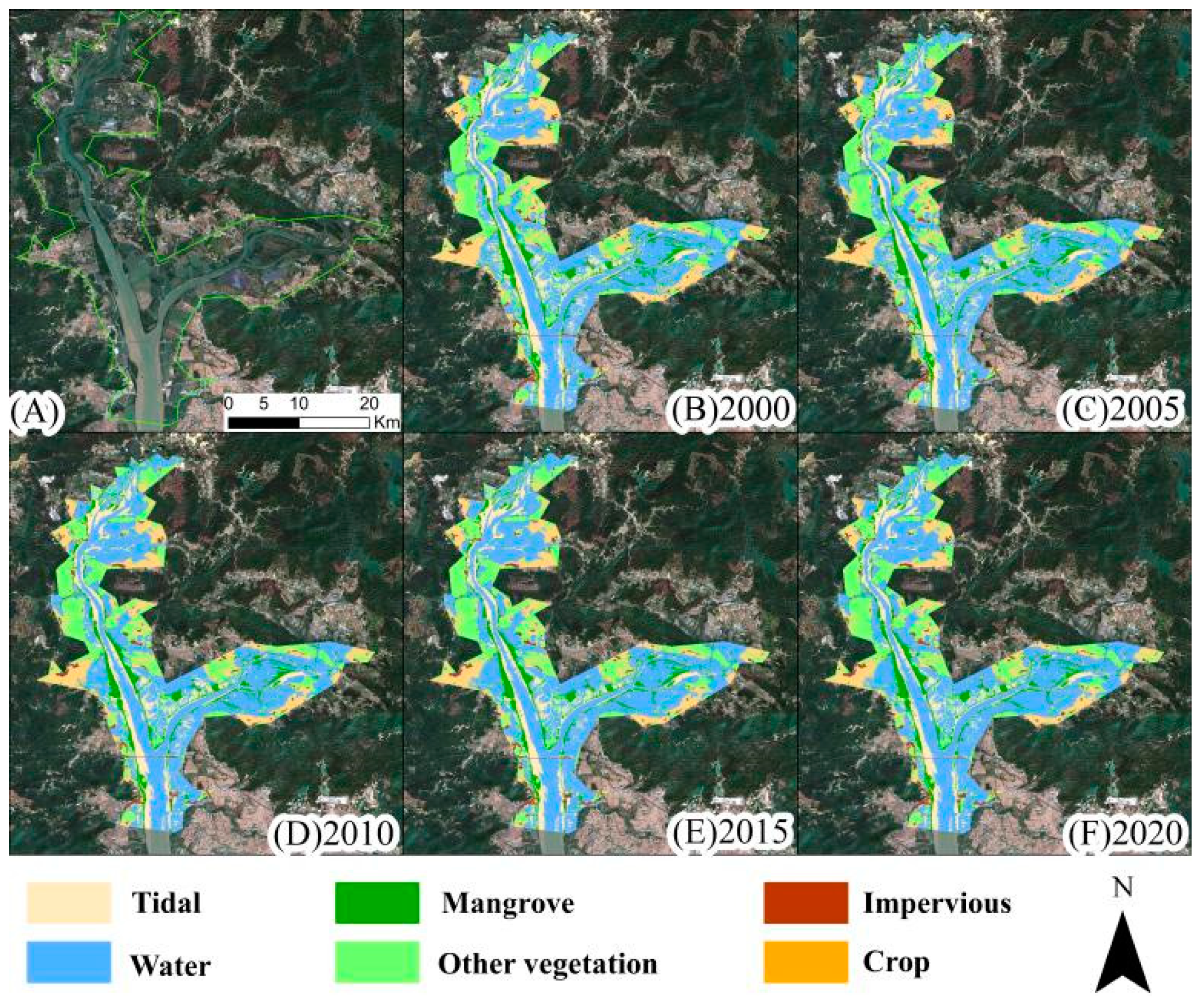
3.2.1. Classification Mapping

This study examines the spatiotemporal changes in mangroves in nature reserves for five years, from 2000 to 2020. The spatiotemporal evolution of mangrove forests in QIMNR and MPMNR is depicted in Figure 5. In the QIMNR and MPMNR, there are obviously more huge patches of mangroves, and the landscape is more connected. Figure A1, Figure A2, Figure A3 and Figure A4 of Appendix A contain further data regarding nature reserves. Figure A3 illustrates the expansion of the FMNNR’s large patch mangrove. Other nature reserves have many small areas of mangroves and mangrove patches that vary widely. Mangroves appear to be broken up more noticeably. Mangrove forests in Nansha expanded to the southwest, mangrove forests in Zhongshan on the west side of the Cuiheng River channel significantly declined, and mangrove forests in Taishan Town Bay were evenly distributed across the nature reserve.

3.2.2. Mangrove Area Dynamics

Table 4 details the temporal and spatial changes in mangrove pixels and their proportion to each nature reserve in the study area from 2000 to 2020. After determining the general size of the nature reserves from the data, remote-sensing extraction was used to determine the entire area (in pixels) of the reserves. When considering the entire mangrove area, in the past 20 years, mangroves have grown in size across the NWP, QIMNR, MPMNR, and FMNNR. In the nature reserves of the GTZMNWP and GZCNWP, the overall area of mangroves has somewhat shrunk. The area of mangroves in the QIMNR increased from 17.785 to 23.743%, and the MPMNR changed from 36.185 to 38.251%. The NWP has experienced significant expansion, with the distribution range drastically growing from 2.419 to 31.247%. However, the area of mangroves in the FMNNR, GTZMNWP, and GZCNWP largely remained or slightly declined.

3.2.3. Mangrove Loss and Gain

As Table 5 lists, in each nature reserve, the proportion of pixels in the mangrove forest changed between 2000 and 2020, suggesting a significant change. The total net change ratio implies that overall mangrove losses outweighed gains in the GTZMNWP and GZCNWP, but overall gains outweighed losses in the NWP, QIMNR, MPMNR, and FMNNR. The percentage of mangroves in the GTZMNWP was basically steady overall. With a net change of −2.771%, the percentage of mangrove pixels in the GZCNWP progressively declined. Mangrove pixels became more widespread over time in the QIMNR, NWP, MPMNR, and FMNNR, with net changes of 5.957%, 28.827%, 2.066%, and 1.309%, respectively. Among these, the NWP was the nature reserve with the largest variety in the mangrove pixels.
Figure 6 suggests mangrove transitions in the QIMNR and MPMNR. The mangrove area in the QIMNR and MPMNR increased significantly. In the QIMNR, a project to introduce and expand mangrove plant communities was implemented. As the introduction of mangroves slowed the growth of Spartina alterniflora, the amount of other vegetation progressively decreased, and mangroves gradually grew. Mangrove protection in the MPMNR was carried out earlier, and the protection measures were relatively effective. Additionally, the MPMNR was not open to the public, greatly reducing human interference, which resulted in a reduced loss of mangroves and a greater conversion of mangroves into other vegetation. However, serious pollution from household, industrial, and agricultural waste has always been the main issue that has kept the Mai Po wetland system from growing healthily. Mangrove loss and gain in other nature reserves can be found in Appendix A, Figure A5 and Figure A6.

3.2.4. Influence of Main Drive Factors on Mangrove

With a significant amount of aquaculture in the GTZMNWP, QIMNR, MPMNR, and GZCNWP with easily distinguishable aquaculture, crop, and impervious area, exploring the causes of mangrove loss can provide an important reference for mangrove conservation. All of this information can be obtained by visually interpreting images. Therefore, the four nature reserves were selected to analyze the effects of aquaculture, crop, and impervious area on mangrove loss in the reserves.
In four nature reserves, the statistical distances between mangroves and impact factors are illustrated in Table A1, Table A2, Table A3 and Table A4. According to the results in the tables, it can be seen that all the mangrove loss in the GTZMNWP occurred within 500 m of aquaculture, with about 90% of the loss occurring within 100 m. The GZCNWP lost all of its mangrove forests within 500 m of crop and impervious area. The percentage of mangrove loss within 500 m of aquaculture in the four time periods of the QIMNR was 59%, 65%, 80%, and 98%, respectively. A tiny percentage of mangroves was lost beyond 500 m of aquaculture because mangrove cultivation has an effect on the mangroves in the nature reserve. The MPMNR lost fewer mangroves, but those losses were mostly within 200 m of aquaculture. In summary, the closer the mangroves in the nature reserve were to artificial ponds, crops and impervious areas, the greater the impact was, and more than 90% occurred within 500 m of artificial ponds, crops, and impervious areas.

3.3. Landscape Pattern of Mangrove

The results of Figure 7 indicate that the fragmentation of nature reserves changed significantly during 2000–2020 and show the spatio-temporal change in mangrove forest fragmentation. Compared to the QIMNR, MPMNR, and FMNNR, the degree of fragmentation in the NWP, GTZMNWP, and GZCNWP was significantly high. The result suggests that the continuity of mangrove forests in the QIMNR, MPMNR, and FMNNR was higher than in the NWP, GTZMNWP, and GZCNWP. The magnitude of the change in NWP was decreased, indicating that the connectivity of mangrove forests in Nansha was increased. The GTZMNWP’s fragmentation pattern was similar to the NWP’s. The FMNNR’s fragmentation had deteriorated, which showed that the connection of the landscape was also declining. This demonstrated that changes in fragmentation were unstable because the number of mangrove patches changed faster. Other nature reserves had only minor and stable fragmentation changes.

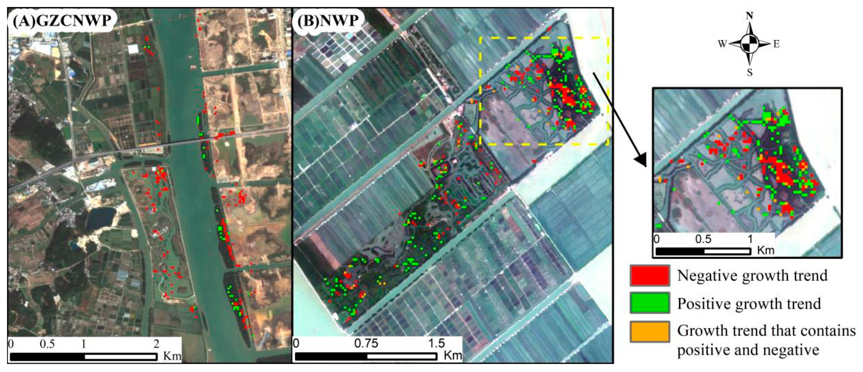
3.4. Mangrove Growth Trends

Figure 8, Figure A7 and Figure A8 indicate the growth trends of stable mangrove forests in the nature reserve from 2000 to 2020. Green means the pixel of the mangrove grew positively. Red means the pixel of the mangrove grew negatively. Orange means the pixel show a positive/negative growth trend and then a negative/positive one. Due to various factors, mangrove growth quality almost changed during 20 years. Therefore, the growth quality of mangroves has been relatively unstable in the 20 years observed. As the change in the mangrove growth trend is spatially fragmented, there are few changes every five years, and there are only two or fewer changes in a period of 20 years. Thus, the change in the mangrove growth trend is shown in a single image. As shown in Figure 9, in the six nature reserves every five years, it is evident that the positive growth trend pixels of mangroves were virtually more than the number of negative pixels, showing that the reserve had an effect on preserving the mangrove growth trends.

3.5. Comprehensive Score Evaluation

Table 6 shows the weight value of each index of nature reserves. The greater the index values changed from 2000 to 2020, the higher the weight values. The weight value of the stable mangrove negative growth trend is the highest of the five indices of the NWP, meaning that there is a great change in stable mangrove negative growth trend. Figure 8 shows this result of the NWP, so there is the highest negative growth trend pixel in NWP in 2015–2020. Meanwhile, it had the fewest positive growth trend pixels. Additionally, the weight of the stable mangrove positive growth trend is the lowest of the five indices of the NWP. Thus, the comprehensive score of the NWP in 2015–2020 is lower. Other nature reserves also found similar results. Consequently, the comprehensive score tends to decline.
Figure 10 depicts the comprehensive evaluation score of the effect of each nature reserve in four time periods, with the result of the conservation effect being relatively acceptable. The overall score of the NWP, GZCNWP, MPMNR, and FMNNR rose and then declined. The overall score of the GTZMNWR and QIMNR tended to decline. The overall score was higher when comparing the mangrove landscape, area, and stable mangrove growth trends of nature reserves, indicating that the mangrove landscape fragmentation was relatively small, and there were relatively more mangrove pixels that grew better and were obtained. The lower overall score indicated the inverse. Compared with the protective effects of different nature reserves, the QIMNR and MPMNR had been relatively poor over the last five years.

4. Discussion

4.1. Driving Factors Analysis of Mangrove Protection Dynamics

The quantitative analysis of the driving factors of mangrove change in this paper can reflect the distance between mangroves and aquaculture, crop, or impervious areas, which can be used to analyze the impact of other factors on mangrove change, as shown in Table A1, Table A2, Table A3 and Table A4. As a result, the greater the losses in the mangroves, the closer they were to these land uses/covers. However, based on experiment results, this transformation between mangroves and these three types of land-use transitions in nature reserves largely did not occur, but some research confirmed that most mangroves were lost to aquaculture and agriculture [3,5,54,55]. Therefore, it is clear that mangrove protection was impacted by the reserve-protection regulations. This demonstrates another influence on the protection of mangroves in the nature reserve. While nature reserve protection and management help reduce the impact of anthropogenic activities on mangroves [9,11,22], this impact indirectly changes the biological and physical processes that affect mangrove reproduction and nutrient transport [56]. Moreover, sea-level rise caused by climate change is the biggest natural threat to mangrove protection [57]. Accordingly, up until 2010, aquaculture, agriculture, and urban development were the biggest threats to mangroves [1,3,5,7]. However, the establishment of nature reserves and afforestation has grown in popularity in the last decade [5]. Thus, when considering nature reserve protection and management, the indirect influence on mangrove, such as the growth trend, appears even more necessary to consider.
Using a land use/cover transition matrix to examine the process and patterns of land use/cover change is a common strategy [58,59,60]. However, the transition is unable to react to the overall change in mangroves. For instance, in Nansha District, mangrove areas increased and the landscape pattern was improved due to the artificial planting of mangroves in 1998 and the subsequent focus on safeguarding mangrove regions in 2014. On the other hand, a negative trend of mangrove growth happened in NWP in 2014, because large-scale development and construction in Nansha District polluted the water of the Pearl River. Thus, the hierarchical evaluation framework for mangrove protection is necessary. Although the mangrove quantity and landscape both improved, suggesting the effect of protection in some aspects, the mangrove growth quality plays a key role in the evaluation process. The comprehensive score of NWP declined obviously after 2015 due to a slow increase in the mangrove area and an increase in negative mangrove growth.
Unlike previous studies, our analysis provides a new perspective (growth trends) for analyzing the potential drivers. The diminishing growth trend leads to lower growth quality, increasing the likelihood of mangrove loss. Due to their tiny areas, significant organic and heavy metal pollution, and adverse effects on mangrove growth trends, the mangroves of FMNNR and NWP have low ecological service functions [61]. Due to these uncertainties, mangroves may grow negatively. There was a large increase in the mangrove area before 2010 in QIMNR, but after that, the negative growth mangrove pixels number declined while the positive opposite and fragmentation changed into bad. Obviously, the comprehensive scores declined from 2000 to 2020 in the QIMNR. Additionally, the MPMNR is a similar case. Thus, we conclude that the protective effect of the QIMNR and MPMNR was relatively poor in the past five years. In general, it is proven that the mangrove growth trends play an important role in analyzing the nature reserve mangrove change. In the future, possible mangrove transitions can be analyzed from the perspective of growth trends.

4.2. Advantages and Limitations of the Evaluation Method

Unlike previous studies, a hierarchical evaluation framework was established to analyze mangrove conservation efforts at three levels. On the one hand, it is feasible to analyze and evaluate mangrove changes and drivers in a few nature reserves by area and landscape [1,22,57]. When the number of reserves is considerable, comparing the effectiveness of the reserves becomes challenging. There are significant differences in disturbed and undisturbed mangrove areas, and mangrove growth quality can impact adjacent ecosystems [62], which in turn affects the health of mangroves. Due to the sensitive effects of mangroves on human activities, this study added the mangrove growth quality to the model and formed a hierarchical evaluation framework. Therefore, this study monitored the disturbed mangroves, distinguishes between positive and negative growth trends of mangroves, and uses them as evaluation indicators. On the other hand, few studies have evaluated mangrove growth quality [23]. Liu et al. conducted a nationwide assessment of the conservation effect of mangrove reserves from a landscape perspective. Jia et al. [18] conducted a national-scale evaluation of the conservation effectiveness, mainly in terms of mangrove areas. Zheng et al. [20] evaluated the conservation effectiveness of China’s national wetland reserves from three aspects: conservation value, wetland changes, and functional zoning adjustment. Although the indicators they used were valid and comprehensive, none considered mangrove growth quality.
Additionally, there are still limitations to the remote-sensing-based hierarchical evaluation framework. It is related to the size of the pixel and accuracy. The detection outcomes are more logical when employing the CCDC algorithm, which applies the per-pixel-model-fitting method to capture seasonal dynamics and inter-year greening and browning trends of various land cover types while also accounting for time correlations [25,34]. However, the discrete pixels may be incorrectly classified as mangrove pixels or some pixels’ missing points may result in mangrove discontinuities [34], which will increase the number of mangrove patches and increase the fragmentation of the overall mangrove landscape. The time series model could be overfitted as well, and three consecutive changes in the atmosphere could result in incorrect classification. However, the CCDC method can achieve high-precision classification, and this study used the conversion of mangroves and other land covers/uses as one of the evaluation elements to reflect the quantitative change in mangroves.
The production accuracy of mangrove areas was 98.94%, user accuracy was 88.57%, and the overall accuracy is 98.71% as shown in Table 3. Zhen et al. [63] used a support vector machine classification method to classify the land use based on a combination of SAR and optical data, with an overall accuracy of 95.04%, a production accuracy of 94.2% and a user accuracy of 96.7%. Jia et al. [22] had an overall accuracy of 92% in the classification of nature reserves in Hong Kong and Shenzhen. Ghorbanian et al. [64] used a random forest classifier within the Google Earth Engine cloud computing platform resulting in an accurate mangrove ecosystem map with an average overall accuracy of 93.23%. Compared with the classification accuracy of these research efforts, the classification accuracy of this study is good. Overall, the obtained classification results are reasonable. It is reasonable that the scores declined because the influence was stressed by mangrove growth trends.
There will be more options in the future for the indicators applied in the hierarchical evaluation framework. At first, mangrove species were not considered in this study. Different mangrove species would show different protection effects. Furthermore, the bird species and the effect of mangrove forests resisting wave disasters, etc., are key factors to express whether the nature reserve affects mangrove protection. Additionally, the data used in this study has a resolution of 30 m. However, the 10 m image data in future studies can provide a more refined research scale, and distinguish the protective effect of different mangrove species through species classification.

5. Conclusions

Using a hierarchical evaluation framework, the effect of mangrove protection and spatiotemporal changes in nature reserves, as well as driving factors, were quantified from time-series remote-sensing images in this study. We found three conclusions for nature reserves of mangroves in the GBA at three levels: (1) From 2000 to 2020, the mangrove forest area rose in the NWP, QIMNR, MPMNR, and FMNNR, while it decreased in GTZMNWP and GZCNWP. The mangrove landscape in nature reserves tends to be more complete and continuous, except for the FMNNR. The positive growth trend of mangroves in the nature reserve is better guaranteed gradually. (2) The establishment of nature reserves and the artificial planting of mangroves were the main causes of mangrove gain. Mangroves have been impacted by human activity in both positive and negative ways. The protection of mangroves in nature reserves increased the size of mangroves, whereas aquaculture activity and its associated effects resulted in some indirect influences on mangroves. (3) The effect of mangrove protection in the six nature reserves tends to be less effective when adding growth trends, according to the results of the comprehensive evaluation scores.
Therefore, the recommendations made in this study for the long-term protection of mangroves in nature reserves mostly focus on maintaining the existing mangroves, continuously expanding the mangrove area, providing a more integrated mangrove landscape, and promoting a positive trend in mangrove growth. Later, mangrove structures then should be considered in the hierarchical evaluation framework. Other important factors, such as mangrove and bird species, should be considered when assessing the protection of mangroves in the future.

Author Contributions

Conceptualization: T.H., Y.F. and W.Z.; methodology: T.H. and H.D.; software: T.H.; validation: T.H., H.D. and X.H.; formal analysis: T.H., Y.F., X.H. and R.L.; writing—original draft preparation: T.H., Y.F., H.D. and S.W.; writing—review and editing: Y.F., H.D., W.Z., X.H. and S.W.; visualization: T.H.; supervision: W.Z.; funding acquisition: Y.F. and H.D. All authors have read and agreed to the published version of the manuscript.

Funding

This work was financially supported by the Natural Science Foundation of China (Nos. 42071399 and 42001329) and the foundation of Luojia1-01 Special Open Research Fund of State Key Laboratory of Information Engineering in Surveying, Mapping and Remote Sensing (No. T1805).

Data Availability Statement

Data from this research will be available upon request to the authors.

Conflicts of Interest

The authors declare no conflict of interest.

Appendix A

The figures of spatiotemporal mangrove change, mangrove transition and growth trends in other nature reserves, and the tables of the distance analysis of driving factors mentioned in this study.
Figure A1. The spatiotemporal changes of mangrove forests in GTZMNWP from 2000 to 2020. (A): the image of GTZMNWP, (B): 2000, (C): 2005, (D): 2010, (E): 2015, (F): 2020.
Remotesensing 14 06026 g0a1
Figure A2. The spatiotemporal changes of mangrove forests in GZCNWP from 2000 to 2020. (A): the image of GZCNWP, (B): 2000, (C): 2005, (D): 2010, (E): 2015, (F): 2020.
Remotesensing 14 06026 g0a2
Figure A3. The spatiotemporal changes of mangrove forests in FMNNR from 2000 to 2020. (A): the image of FMNNR, (B): 2000, (C): 2005, (D): 2010, (E): 2015, (F): 2020.
Remotesensing 14 06026 g0a3
Figure A4. The spatiotemporal changes of mangrove forests in NWP from 2000 to 2020. (A): the image of NWP, (B): 2000, (C): 2005, (D): 2010, (E): 2015, (F): 2020.
Remotesensing 14 06026 g0a4
Figure A5. Mangrove gain and loss in GZCNWP(AD) and NWP(EH) every five years from 2000 to 2020. (A,E): 2000–2005, (B,F): 2005–2010, (C,G): 2010–2015, (D,H): 2015–2020.
Remotesensing 14 06026 g0a5
Figure A6. Mangrove gain and loss in FMNNR(AD) and GTZMNWP(EH) every five years from 2000 to 2020. (A,E): 2000–2005, (B,F): 2005–2010, (C,G): 2010–2015, (D,H): 2015–2020.
Remotesensing 14 06026 g0a6
Figure A7. The growth trends of stable mangroves occurred in (A) GZCNWP and (B) NWP in 2000–2020.
Remotesensing 14 06026 g0a7
Figure A8. The growth trends of stable mangroves occurred in (A) GTZMNWP and (B) FMNNR in 2000–2020.
Remotesensing 14 06026 g0a8
Table A1. The quantity relationship of lost mangrove pixels and the distances between mangroves and driving factors in GTZMNWP.
GTZMNWP
Pixel
m
D ≤ 50 50 < D ≤ 100 100 < D ≤ 200 200 < D ≤ 500 500 < D
2000–200514316500
2005–20103138920
2010–201517024860
2015–20201627548150
Table A2. The quantity relationship of lost mangrove pixels and the distances between mangroves and driving factors in GZCNWP.
GZCNWP
Pixel
m
D ≤ 50 50 < D ≤ 100 100 < D ≤ 200 200 < D ≤ 500 500 < D
2000–2005167201750
2005–2010478200
2010–2015111100
2015–2020551000
Table A3. The quantity relationship of lost mangrove pixels and the distances between mangroves and driving factors in QIMNR.
QIMNR
Pixel
m
D ≤ 50 50 < D ≤ 100 100 < D ≤ 200 200 < D ≤ 500 500 < D ≤ 1000 1000 < D
2000–2005731217
2005–2010814666
2010–2015521220
2015–20208971810
Table A4. The quantity relationship of lost mangrove pixels and the distances between mangroves and driving factors in MPMNR.
MPMNR
Pixel
m
D ≤ 50 50 < D ≤ 100 100 < D ≤ 200 200 < D ≤ 500 500 < D
2000–200541000
2005–201000100
2010–201500000
2015–202051101

References

  1. Wang, H.; Peng, Y.; Wang, C.; Wen, Q.; Xu, J.; Hu, Z.; Jia, X.; Zhao, X.; Lian, W.; Temmerman, S.; et al. Mangrove Loss and Gain in a Densely Populated Urban Estuary: Lessons From the Guangdong-Hong Kong-Macao Greater Bay Area. Front. Mar. Sci. 2021, 8, 693450. [Google Scholar] [CrossRef]
  2. Carugati, L.; Gatto, B.; Rastelli, E.; Lo Martire, M.; Coral, C.; Greco, S.; Danovaro, R. Impact of mangrove forests degradation on biodiversity and ecosystem functioning. Sci. Rep. 2018, 8, 13298. [Google Scholar] [CrossRef]
  3. Goldberg, L.; Lagomasino, D.; Thomas, N.; Fatoyinbo, T. Global declines in human-driven mangrove loss. Glob. Chang. Biol. 2020, 26, 5844–5855. [Google Scholar] [CrossRef] [PubMed]
  4. Murray, N.J.; Worthington, T.; Bunting, P.; Duce, S.; Hagger, V.; Lovelock, C.; Lucas, R.; Saunders, M.I.; Sheaves, M.; Spalding, M.; et al. High-resolution mapping of losses and gains of Earth’s tidal wetlands. Science 2022, 376, 744–749. [Google Scholar] [CrossRef]
  5. Friess, D.A.; Rogers, K.; Lovelock, C.E.; Krauss, K.W.; Hamilton, S.E.; Lee, S.Y.; Lucas, R.; Primavera, J.; Rajkaran, A.; Shi, S. The State of the World’s Mangrove Forests: Past, Present, and Future. Annu. Rev. Environ. Resour. 2019, 44, 89–115. [Google Scholar] [CrossRef]
  6. Fu, X.; Tang, H.; Liu, Y.; Zhang, M.; Jiang, S.; Yang, F.; Li, X.; Wang, C. Resource status and protection strategies of mangroves in China. J. Coast. Conserv. 2021, 25, 42. [Google Scholar] [CrossRef]
  7. Thomas, N.; Lucas, R.; Bunting, P.; Hardy, A.; Rosenqvist, A.; Simard, M. Distribution and drivers of global mangrove forest change, 1996–2010. PLoS ONE 2017, 12, e0179302. [Google Scholar] [CrossRef] [PubMed]
  8. Almeida, L.T.D.; Olímpio, J.L.S.; Pantalena, A.F.; Almeida, B.S.D.; Oliveira Soares, M.D. Evaluating ten years of management effectiveness in a mangrove protected area. Ocean Coast. Manag. 2016, 125, 29–37. [Google Scholar] [CrossRef]
  9. Miteva, D.A.; Murray, B.C.; Pattanayak, S.K. Do protected areas reduce blue carbon emissions? A quasi-experimental evaluation of mangroves in Indonesia. Ecol. Econ. 2015, 119, 127–135. [Google Scholar] [CrossRef]
  10. Cavalcanti, V.F.; Soares, M.L.G.; Estrada, G.C.D.; Chaves, F.O. Evaluating Mangrove Conservation through the Analysis of Forest Structure Data. J. Coast. Res. 2009, 1, 390–394. [Google Scholar]
  11. Ribas, L.G.d.S.; Pressey, R.L.; Loyola, R.; Bini, L.M. A global comparative analysis of impact evaluation methods in estimating the effectiveness of protected areas. Biodivers. Conserv. 2020, 246, 108595. [Google Scholar] [CrossRef]
  12. Matthews, G.V.T. The Ramsar Covention on Wetlands; Its History and Development; Secretariat, R.C., Ed.; Imprimerie Dupuis SA: Gland, Switzerland, 2013; pp. 4–7. [Google Scholar]
  13. Fang, B.X.; Dan, X.Q. Chinese mangrove resources and protection. Cent. South For. Inventory Plan. 2001, 20, 25–30, 33. [Google Scholar]
  14. Chen, L.; Wang, W.; Zhang, Y.; Lin, G. Recent progresses in mangrove conservation, restoration and research in China. J. Plant Ecol. 2009, 2, 45–54. [Google Scholar] [CrossRef]
  15. Rodrigues, A.S.L.; Cazalis, V. The multifaceted challenge of evaluating protected area effectiveness. Nat. Commun. 2020, 11, 5147. [Google Scholar] [CrossRef] [PubMed]
  16. Bryan-Brown, D.N.; Connolly, R.M.; Richards, D.R.; Adame, F.; Friess, D.A.; Brown, C.J. Global trends in mangrove forest fragmentation. Sci. Rep. 2020, 10, 7117. [Google Scholar] [CrossRef]
  17. Luo, S.; Chui, T.F. Annual variations in regional mangrove cover in southern China and potential macro-climatic and hydrological indicators. Ecol. Indic. 2020, 110, 105927. [Google Scholar] [CrossRef]
  18. Jia, M.; Wang, Z.; Zhang, Y.; Mao, D.; Wang, C. Monitoring loss and recovery of mangrove forests during 42 years: The achievements of mangrove conservation in China. Int. J. Appl. Earth. Obs. Geoinf. 2018, 73, 535–545. [Google Scholar] [CrossRef]
  19. Shah, P.; Baylis, K.; Busch, J.; Engelmann, J. What determines the effectiveness of national protected area networks? Environ. Res. Lett. 2021, 16, 074017. [Google Scholar] [CrossRef]
  20. Zheng, Y.; Zhang, H.; Niu, Z.; Gong, P. Protection efficacy of national wetland reserves in China. Chin. Sci. Bull. 2012, 57, 1116–1134. [Google Scholar] [CrossRef]
  21. Tue, N.T.; Dung, L.V.; Nhuan, M.T.; Omori, K. Carbon storage of a tropical mangrove forest in Mui Ca Mau National Park, Vietnam. Catena 2014, 121, 119–126. [Google Scholar] [CrossRef]
  22. Jia, M.; Liu, M.; Wang, Z.; Mao, D.; Ren, C.; Cui, H. Evaluating the Effectiveness of Conservation on Mangroves: A Remote Sensing-Based Comparison for Two Adjacent Protected Areas in Shenzhen and Hong Kong, China. Remote Sens. 2016, 8, 627. [Google Scholar] [CrossRef]
  23. Borges, R.; Ferreira, A.C.; Lacerda, L.D. Systematic Planning and Ecosystem-Based Management as Strategies to Reconcile Mangrove Conservation with Resource Use. Front. Mar. Sci. 2017, 4, 353. [Google Scholar] [CrossRef] [Green Version]
  24. Geldmann, J.; Manica, A.; Burgess, N.D.; Coad, L.; Balmford, A. A global-level assessment of the effectiveness of protected areas at resisting anthropogenic pressures. Proc. Natl. Acad. Sci. USA 2019, 116, 23209–23215. [Google Scholar] [CrossRef]
  25. Zhu, Z.; Fu, Y.; Woodcock, C.E.; Olofsson, P.; Vogelmann, J.E.; Holden, C.; Wang, M.; Dai, S.; Yu, Y. Including land cover change in analysis of greenness trends using all available Landsat 5, 7, and 8 images: A case study from Guangzhou, China (2000–2014). Remote Sens. Environ. 2016, 185, 243–257. [Google Scholar] [CrossRef]
  26. Loveland, T.R.; Anderson, M.C.; Huntington, J.L.; Irons, J.R.; Johnson, D.M.; Rocchio, L.E.P.; Woodcock, C.E.; Wulder, M.A. Seeing Our Planet Anew: Fifty Years of Landsat. Photogramm. Eng. Remote Sens. 2022, 88, 429–436. [Google Scholar] [CrossRef]
  27. Wulder, M.A.; Roy, D.P.; Radeloff, V.C.; Loveland, T.R.; Anderson, M.C.; Johnson, D.M.; Healey, S.; Zhu, Z.; Scambos, T.A.; Pahlevan, N.; et al. Fifty years of Landsat science and impacts. Remote Sens. Environ. 2022, 280, 113195. [Google Scholar] [CrossRef]
  28. Nguyen, T.H.; Jones, S.; Soto-Berelov, M.; Haywood, A.; Hislop, S. Landsat Time-Series for Estimating Forest Aboveground Biomass and Its Dynamics across Space and Time: A Review. Remote Sens. 2019, 12, 98. [Google Scholar] [CrossRef]
  29. Zhou, C.; Wei, X.; Zhou, G.; Yan, J.; Wang, X.; Wang, C.; Liu, H.; Tang, X.; Zhang, Q. Impacts of a large-scale reforestation program on carbon storage dynamics in Guangdong, China. For. Ecol. Manag. 2008, 255, 847–854. [Google Scholar] [CrossRef]
  30. Li, J.; Wang, F.; Fu, Y.; Guo, B.; Zhao, Y.; Yu, H. A Novel SUHI Referenced Estimation Method for Multicenters Urban Agglomeration using DMSP/OLS Nighttime Light Data. IEEE J. Sel. Top. Appl. Earth Obs. Remote Sens. 2020, 13, 1416–1425. [Google Scholar] [CrossRef]
  31. Zhao, J.; Yu, L.; Xu, Y.; Ren, H.; Huang, X.; Gong, P. Exploring the addition of Landsat 8 thermal band in land-cover mapping. Int. J. Remote Sens. 2019, 40, 4544–4559. [Google Scholar] [CrossRef]
  32. Ghosh, S.; Mishra, D.R.; Gitelson, A.A. Long-term monitoring of biophysical characteristics of tidal wetlands in the northern Gulf of Mexico—A methodological approach using MODIS. Remote Sens. Environ. 2016, 173, 39–58. [Google Scholar] [CrossRef]
  33. Li, Z.; Feng, Y.; Dessay, N.; Delaitre, E.; Gurgel, H.; Gong, P. Continuous Monitoring of the Spatio-Temporal Patterns of Surface Water in Response to Land Use and Land Cover Types in a Mediterranean Lagoon Complex. Remote Sens. 2019, 11, 1425. [Google Scholar] [CrossRef] [Green Version]
  34. Zhu, Z.; Woodcock, C.E. Continuous change detection and classification of land cover using all available Landsat data. Remote Sens. Environ. 2014, 144, 152–171. [Google Scholar] [CrossRef]
  35. Wang, X.; Li, R.; Ding, H.; Fu, Y. Fine-Scale Improved Carbon Bookkeeping Model Using Landsat Time Series for Subtropical Forest, Southern China. Remote Sens. 2022, 14, 753. [Google Scholar] [CrossRef]
  36. Awty-Carroll, K.; Bunting, P.; Hardy, A.; Bell, G. Using Continuous Change Detection and Classification of Landsat Data to Investigate Long-Term Mangrove Dynamics in the Sundarbans Region. Remote Sens. 2019, 11, 2833. [Google Scholar] [CrossRef]
  37. Fu, Y.C.; Yu, Y. Exploring the greening trends in Guangzhou in recently 15 years using all available Landsat’s images. IGARSS 2016, 7, 2312–2315. [Google Scholar]
  38. Zhu, Z.; Woodcock, C.E.; Olofsson, P. Continuous monitoring of forest disturbance using all available Landsat imagery. Remote Sens. Environ. 2012, 122, 75–91. [Google Scholar] [CrossRef]
  39. Edwards, D.P.; Larsen, T.H.; Docherty, T.D.; Ansell, F.A.; Hsu, W.W.; Derhe, M.A.; Hamer, K.C.; Wilcove, D.S. Degraded lands worth protecting: The biological importance of Southeast Asia’s repeatedly logged forests. Proc. Biol. Sci. 2011, 278, 82–90. [Google Scholar] [CrossRef]
  40. Hwang, C.L.; Yoon, K. Multiple Attribute Decision Making: Methods and Applications, 1st ed.; Springer: Berlin/Heidelberg, Germany, 2011. [Google Scholar]
  41. Min, W.; Shuhao, L. Research on the measurement of China’s high quality economic development level in the new era. Res. Quant. Econ. Technol. Econ. 2018, 35, 3–20. [Google Scholar]
  42. Zuo, Q.T.; Zhang, Z.Z.; Wu, B.B. Evaluation of Water Resources carrying capacity of the Yellow River Basin based on combined weight TOPSIS model. Water Resour. Prot. 2020, 36, 1–7. [Google Scholar]
  43. Wu, H.Y.; Liu, W.Q.; Zheng, J.; Li, C.M. Summary of the Climate of Guangdong Province in 2015. Guangdong Meteorol. 2016, 38, 1–5. [Google Scholar]
  44. Zhao, C.; Qin, C.-Z.; Teng, J. Mapping large-area tidal flats without the dependence on tidal elevations: A case study of Southern China. ISPRS J. Photogramm. Remote Sens. 2020, 159, 256–270. [Google Scholar] [CrossRef]
  45. Masek, J.G.; Vermote, E.F.; Saleous, N.E.; Wolfe, R.; Hall, F.G.; Huemmrich, K.F.; Gao, F.; Kutler, J.; Lim, T.K. A Landsat Surface Reflectance Dataset for North America, 1990–2000. IEEE Geosci. Remote Sens. Lett. 2006, 3, 68–72. [Google Scholar] [CrossRef]
  46. Chen, B.; Xiao, X.; Li, X.; Pan, L.; Doughty, R.; Ma, J.; Dong, J.; Qin, Y.; Zhao, B.; Wu, Z.; et al. A mangrove forest map of China in 2015: Analysis of time series Landsat 7/8 and Sentinel-1A imagery in Google Earth Engine cloud computing platform. ISPRS J. Photogramm. Remote Sens. 2017, 131, 104–120. [Google Scholar] [CrossRef]
  47. Lee, S.Y.; Hamilton, S.; Barbier, E.B.; Primavera, J.; Lewis, R.R. 3rd Better restoration policies are needed to conserve mangrove ecosystems. Nat. Ecol. Evol. 2019, 3, 870–872. [Google Scholar] [CrossRef] [PubMed]
  48. Suyadi; Gao, J.; Lundquist, C.J.; Schwendenmann, L. Characterizing landscape patterns in changing mangrove ecosystems at high latitudes using spatial metrics. Estuar. Coast. Shelf Sci. 2018, 215, 1–10. [Google Scholar] [CrossRef]
  49. Zhu, Z.; Woodcock, C.E.; Holden, C.; Yang, Z. Generating synthetic Landsat images based on all available Landsat data: Predicting Landsat surface reflectance at any given time. Remote Sens. Environ. 2015, 162, 67–83. [Google Scholar] [CrossRef]
  50. Cochran, W.G. Sampling techniques, 3rd ed.; John Wiley & Sons: New York, NY, America, 1977. [Google Scholar]
  51. Olofsson, P.; Foody, G.M.; Stehman, S.V.; Woodcock, C.E. Making better use of accuracy data in land change studies: Estimating accuracy and area and quantifying uncertainty using stratified estimation. Remote Sens. Environ. 2013, 129, 122–131. [Google Scholar] [CrossRef]
  52. Olofsson, P.; Foody, G.M.; Herold, M.; Stehman, S.V.; Woodcock, C.E.; Wulder, M.A. Good practices for estimating area and assessing accuracy of land change. Remote Sens. Environ. 2014, 148, 42–57. [Google Scholar] [CrossRef]
  53. Wu, J.G. Landscape Ecology: Pattern, Process, Scale and Hierarchy, 2nd ed.; Higher Education Press: Beijing, China, 2007; pp. 106–121. [Google Scholar]
  54. Bunting, P.; Rosenqvist, A.; Hilarides, L.; Lucas, R.M.; Thomas, N.; Tadono, T.; Worthington, T.A.; Spalding, M.; Murray, N.J.; Rebelo, L.-M. Global Mangrove Extent Change 1996–2020: Global Mangrove Watch Version 3.0. Remote Sens. 2022, 14, 3657. [Google Scholar] [CrossRef]
  55. Richards, D.R.; Friess, D.A. Rates and drivers of mangrove deforestation in Southeast Asia, 2000–2012. Proc. Natl. Acad. Sci. USA 2016, 113, 344–349. [Google Scholar] [CrossRef] [PubMed]
  56. Critchley, L.P.; Bugnot, A.B.; Dafforn, K.A.; Marzinelli, E.M.; Bishop, M.J. Comparison of wrack dynamics between mangrove forests with and without seawalls. Sci. Total. Environ. 2021, 751, 141371. [Google Scholar] [CrossRef] [PubMed]
  57. Feng, Z.; Tan, G.; Xia, J.; Shu, C.; Chen, P.; Wu, M.; Wu, X. Dynamics of mangrove forests in Shenzhen Bay in response to natural and anthropogenic factors from 1988 to 2017. J. Hydrol. 2020, 591, 125271. [Google Scholar] [CrossRef]
  58. Hu, Y.; Batunacun; Zhen, L.; Zhuang, D. Assessment of Land-Use and Land-Cover Change in Guangxi, China. Sci. Rep. 2019, 9, 2189. [Google Scholar] [CrossRef] [PubMed]
  59. Zhu, B.; Liao, J.; Shen, G. Combining time series and land cover data for analyzing spatio-temporal changes in mangrove forests: A case study of Qinglangang Nature Reserve, Hainan, China. Ecol. Indic. 2021, 131, 108135. [Google Scholar] [CrossRef]
  60. Zheng, Y.; Takeuchi, W. Quantitative Assessment and Driving Force Analysis of Mangrove Forest Changes in China from 1985 to 2018 by Integrating Optical and Radar Imagery. ISPRS Int. J. Geoinf. 2020, 9, 513. [Google Scholar] [CrossRef]
  61. Zhang, Y.Q.; Zhang, Z.; Jiang, B.Q.; Shen, X.Y.; Li, R.L. Ecosystem health assessment and management strategies of typical urban mangroves in Guangdong-Hongkog-Macao Greater Bay Area. China Environ. Sci. 2022, 42, 2352–2369. [Google Scholar]
  62. Geldmann, J.; Coad, L.; Barnes, M.; Craigie, I.D.; Hockings, M.; Knights, K.; Leverington, F.; Cuadros, I.C.; Zamora, C.; Woodley, S.; et al. Changes in protected area management effectiveness over time: A global analysis. Biol. Conserv. 2015, 191, 692–699. [Google Scholar] [CrossRef]
  63. Zhen, J.; Liao, J.; Shen, G. Mapping Mangrove Forests of Dongzhaigang Nature Reserve in China Using Landsat 8 and Radarsat-2 Polarimetric SAR Data. Sensors 2018, 18, 4012. [Google Scholar] [CrossRef]
  64. Ghorbanian, A.; Zaghian, S.; Asiyabi, R.M.; Amani, M.; Mohammadzadeh, A.; Jamali, S. Mangrove Ecosystem Mapping Using Sentinel-1 and Sentinel-2 Satellite Images and Random Forest Algorithm in Google Earth Engine. Remote Sens. 2021, 13, 2565. [Google Scholar] [CrossRef]
Figure 1. The geographical locations of GBA and nature reserves. (A) GTZMNWP, (B) GTZMNWP, (C) GZCNWP, (D) NWP, (E) FMNNR, (F) MPMNR.
Remotesensing 14 06026 g001
Figure 2. The flowchart of the research.
Remotesensing 14 06026 g002
Figure 3. The locations of validation samples.
Remotesensing 14 06026 g003
Figure 4. The criteria for judging stable mangrove positive and negative growth trends.
Remotesensing 14 06026 g004
Figure 5. The spatiotemporal changes of mangrove forests in MPMNR (AF) and QIMNR (GL) from 2000 to 2020. (A,G): the image of MPMNR and QIMNR, (B,H): 2000, (C,I): 2005, (D,J): 2010, (E,K): 2015, (F,L): 2020.
Remotesensing 14 06026 g005
Figure 6. Mangrove gain and loss in nature reserves every five years from 2000 to 2020. The MPMNR is on the top and the QIMNR is on the below. (A,E): 2000–2005, (B,F): 2005–2010, (C,G): 2010–2015, (D,H): 2015–2020.
Remotesensing 14 06026 g006
Figure 7. Fragmentation change of mangrove forests for nature reserves from 2000 to 2020.
Remotesensing 14 06026 g007
Figure 8. The growth trends of stable mangroves occurred in (A) MPMNR and (B) QIMNR in 2000–2020.
Remotesensing 14 06026 g008
Figure 9. The pixel number of growth trends of stable mangroves in six nature reserves from 2000 to 2020; (A) the pixel number of positive growth trends, (B) the pixel number of negative growth trends.
Remotesensing 14 06026 g009
Figure 10. Comprehension scores ( C i ) of nature reserves from 2000 to 2020.
Remotesensing 14 06026 g010
Table 1. Overview of the features used for mapping terraces.
Name of ReserveLocation Climate Conditions
Conservation Areas (ha)Starting Time Protection TypeAnnual Average Temperature (℃)Annual Average Precipitation (mm)Climate Type
NWP22°26′–23°6′N
113°13′–113°43′E
626.72014Local21.81635.6South Asian subtropical ocean monsoon climate
GTZMNWP21°44′–21°56′30″N
112°24′–112°33′E
10,0802004Local21.3~22.82183.3Tropical monsoon climate
GZCNWP22°30′–22°32′N
113°34′–113°35′E
625.62017National21.61731Tropical monsoon climate
FMNNR114°03′E, 22°32′N3681984National22.551926.8Sub-tropical maritime climate
MPMNR113°59′–114°03′E,
22°29′–22°31′N
15001983National22.551926.8South Asian tropical monsoon climate
QIMNR113°36′40″–113°39′15″E
22°23′40″–22°27′38″N
5103.771999Provincial--Tropical monsoon climate
Table 2. Definitions of 6 types of land use in this study.
Land Cover TypeExample ImageDefinition
MangroveRemotesensing 14 06026 i001Growing mangrove plant communities with no obvious bare land or tidal flats
WaterRemotesensing 14 06026 i002Aquaculture without mangroves on the surface and base, seawater, rivers, and the landscape water inside the city
ImperviousRemotesensing 14 06026 i003Unutilized land, artificial features (such as villages, roads, and other construction land), or large tracts of wasteland partially occupied by construction
Other vegetationRemotesensing 14 06026 i004The vegetation distributed in the suitable area of mangroves except for mangrove, including plants in cities, green plants near pond bases, and natural forest vegetation
CropRemotesensing 14 06026 i005Vegetation with a distinct stripped texture, green or light green in color
TidalRemotesensing 14 06026 i006Bare tidal with a clear separation from the water
Table 3. Accuracy assessment and area mapping for stable land cover and mangrove loss and gain from 2000 to 2020.
ClassGround Truth(Pixels)
CropOther VegetationImperviousMangroveTidalWaterMangrove LossMangrove GainTotalMap AREA [ha]
Crop9310004009879,156.70
Other vegetation4416400400428434,893.60
Impervious1117600100179165,427.31
Mangrove040621021702455.08
Tidal000049000499302.18
Water0010060200603966,564.66
Mangrove loss060020202301099.85
Mangrove gain03010032330699.61
Total984311816352611252614871,659,598.98
Area-estimation
(ha)
80,106.69424,862.43168,322.142197.829410.57973,181.22873.34644.761,659,598.98
Overall accuracy98.71%
user accuracy94.90%97.20%98.32%88.57%100%99.83%66.67%76.67%
producer accuracy93.77%99.49%96.63%98.94%98.85%99.16%83.96%83.19%
Table 4. Mangrove proportion of total pixels in nature reserves.
Nature ReserveTotal Pixel20002005201020152020
Pixel%Pixel%Pixel%Pixel%Pixel%
NWP54151312.41974313.721148627.442166030.656169231.247
GTZMNWP147,62911,1547.55511,1627.56110,8967.38110,7487.28010,7077.253
GZCNWP747088511.8476959.3046889.2107169.5856789.076
QIMNR24,357433217.785534221.932570523.422577623.714578323.743
MPMNR9001325736.185329636.618341537.940343438.151344338.251
FMNNR5804136623.535137223.639138423.846141624.397144224.845
Table 5. The Proportion of Mangrove Changing Pixels in Each Nature Reserve.
Change (%)2000–20052005–20102010–20152015–2020Total Net Change (%)
NWP11.30213.7213.2130.59128.827
GTZMNWP0.005−0.180−0.100−0.028−0.303
GZCNWP−2.544−0.0940.375−0.509−2.771
QIMNR4.1471.4900.2910.0295.957
MPMNR0.4331.3220.2110.1002.066
FMNNR0.1030.2070.5510.4481.309
Table 6. The weight of each index of nature reserves.
WeightFMGSMPMLSMN
NWP0.2150.2150.1750.1780.217
GTZMNWP0.1890.2150.1890.1960.211
GZCNWP0.1500.1640.2280.2090.248
QIMNR0.1570.2410.1790.1740.249
MPMNR0.1600.2210.1910.2520.177
FMNNR0.1710.1900.1740.2300.235
Publisher’s Note: MDPI stays neutral with regard to jurisdictional claims in published maps and institutional affiliations.

