Article

Comparison of Model-Assisted Endogenous Poststratification Methods for Estimation of Above-Ground Biomass Change in Oregon, USA

1
Forest Biometrics and Measurements Laboratory, Department Forest Engineering, Resources and Management, Oregon State University, Corvallis, OR 97331, USA
2
US Forest Service Pacific Northwest Research Station, 3200 SW Jefferson Way, Corvallis, OR 97331, USA
3
US Forest Service, Rocky Mountain Research Station, 1221 S Main St, Moscow, ID 83843, USA
4
Natural Resource Ecology Laboratory, Colorado State University, Fort Collins, CO 80523, USA
5
US Forest Service Rocky Mountain Research Station, Ogden, UT 84401, USA
*
Author to whom correspondence should be addressed.
Current address: Cambium Research Group, Área de Producción Vegetal, Departmento de Ciencias Agroforestales, EiFAB-iuFOR, Campus Duques de Soria s/n, ES-42004 Soria, Spain.
Remote Sens. 2022, 14(23), 6024; https://doi.org/10.3390/rs14236024
Submission received: 14 October 2022 / Revised: 22 November 2022 / Accepted: 23 November 2022 / Published: 28 November 2022
(This article belongs to the Collection Feature Paper Special Issue on Forest Remote Sensing)

Abstract

:
Quantifying above-ground biomass changes, ΔAGB, is key for understanding carbon dynamics. National Forest Inventories, NFIs, aims at providing precise estimates of ΔAGB relying on model-assisted estimators that incorporate auxiliary information to reduce uncertainty. Poststratification estimators, PS, are commonly used for this task. Recently proposed endogenous poststratification, EPS, methods have the potential to improve the precision of PS estimates of ΔAGB. Using the state of Oregon, USA, as a testing area, we developed a formal comparison between three EPS methods, traditional PS estimators used in the region, and the Horvitz-Thompson, HT, estimator. Results showed that gains in performance with respect to the HT estimator were 9.71% to 19.22% larger for EPS than for PS. Furthermore, EPS methods easily accommodated a large number of auxiliary variables, and the inclusion of independent predictions of ΔAGB as an additional auxiliary variable resulted in further gains in performance.

1. Introduction

National forest inventories, NFIs, collect measurements and provide the necessary infrastructure to estimate the state and dynamics of the forested areas of their respective countries [1]. To satisfy the demands of information posed by society, national legislation, or international agreements, NFIs have to allow the estimation of means and totals of a large and increasing number of variables of a very different nature [1,2,3]. While NFI sampling designs can vary substantially between countries (see [3]), several features are common to most NFIs. Sampling designs of NFIs typically use systematic or near-systematic approaches [4] based on regular grids, and measurements of field plots are organized over time in a systematic and cyclic fashion. This ensures that samples are spatially balanced [5] and at least a fraction of the field plots are revisited at a frequency that enables NFIs to estimate changes in ecologically important attributes [1,3]. The resulting sampling designs are generalist and standardized within countries; and making possible the estimation of the state and dynamics for multiple forest attributes and facilitating comparisons between spatial domains or time periods is typically considered a priority.
The large degree of standardization and the generality that allow NFI sampling designs to estimate many attributes also implies that they are not optimized in terms of precision for any particular variable [3]. Therefore, the uncertainty of estimates for specific variables can be large. This problem is typically addressed using estimators that incorporate auxiliary information to gain precision in the estimation of key variables. While model-based estimators [6] could be used for this purpose, model-assisted estimators such as generalized regression estimators, GREG, post-stratification estimators, PS, or calibration estimators are typically the preferred choice. This is because model-assisted estimators: (1) allow using abundant sources of auxiliary information to improve the precision in the estimation process [7] and (2) do not involve strong assumptions about the structure of the population of interest in the shape of regression models being approximately unbiased even if the assisting models are not correctly specified [7].
In the NFI of the United States of America, the US Forest Service Forest Inventory and Analysis program, FIA, PS is typically used to estimate both state and dynamic variables. In the Pacific Northwest FIA region, PNW-FIA (i.e., states of Alaska, Hawaii, Oregon, Washington, and California, and the Pacific Island territories), the PS currently used for all variables was developed using expert opinion based on ownership, ownership size, canopy cover, and a classification into forest, non-forest and unknown. PNW-FIA has used the resulting PS during the last 7 years, and it has proven to satisfy the reporting standards of FIA for state variables such as above-ground tree biomass, AGB, or volume, even when disaggregating by broad size or species classes or by large geographical domains such as states or large counties. The auxiliary variables used to develop this PS are primarily static descriptors, and when this PS is used to estimate the change in forest AGB, Δ A G B , the precision of the PS estimators declines substantially. A potential solution to this lack of precision is developing new model-assisted estimators with dynamic auxiliary variables specially tailored to improve the precision for change variables. However, several features must be analyzed before a model-assisted estimator and a set of auxiliary variables are incorporated into the FIA protocols.
Model-assisted techniques yield improvements in precision that are directly related to the correlation between auxiliary variables and target response. Thus, a cornerstone for developing a new estimator for Δ A G B is the identification of auxiliary variables potentially correlated to this variable. Positive Δ A G B (i.e., an increase) can be expected to be the result of steady growth dynamics. In contrast, negative Δ A G B can result from steady decline dynamics (i.e., senescence or slow diseases) or from events of varying intensity, such as insect outbreaks, fires, or harvest operations such as thinning or clear-cuts. Thus, rather than using a single auxiliary variable, a model-assisted estimator for Δ A G B will require multiple and complementary auxiliary variables capturing information about the different drivers of change.
Numerous sources of auxiliary variables potentially correlated to factors affecting Δ A G B are currently available. However, the potential correlation with Δ A G B cannot be the only factor under consideration. Before a source of auxiliary information is considered appropriate for developing new model-assisted estimators, it must meet some standards in terms of spatial coverage, temporal extent, and update frequency. Otherwise, compatibility with the 10-year rotating panel design of the PNW-FIA region and harmonization with current reporting practices could become infeasible. These considerations are especially relevant for recent remote sensing products that: use Landsat time series and topographic and climate variables to provide yearly predictions of AGB and that are developed using ground observations that are independent of the FIA sampling design [8,9]. By differencing AGB predictions from specific years, it is possible to derive predictions of ΔAGB that are highly correlated with actual ΔAGB. These predictions of ΔAGB can be used as auxiliary variables that encode, in a single auxiliary variable, the most relevant information provided by the remote sensing datasets used in their construction. These datasets are very recent, but their potential correlation with Δ A G B and the fact that they were derived with ground data independent of FIA, call for investigations about their use in FIA estimation.
Some model-assisted estimators have been developed and could be used to improve the precision of estimates of Δ A G B . However, we will focus the remainder of this manuscript on PS estimators. These estimators can be seen as a sub-type of GREG estimators where the auxiliary variables are stratum-membership indicator variables [7]. From an operational perspective, PS estimators are the most appealing alternative because they imply a continuation of the methods currently used in the region, which is an important advantage of PS over more general formulations of GREG estimators. In addition, PS estimators can account for differences in sampling intensities between strata that occur after denial of access to plot locations or hazardous plot conditions. Additionally, PS estimators have a large degree of flexibility and ensure compatibility (i.e., positive weights are ensured) with the design of the FIA database and associated software [10].
Several alternatives exist to develop a PS estimator. Traditional PS methods in PNW-FIA have used expert knowledge and geographic information systems, GIS, and data about forest types, ownership, administrative boundaries, etc., to define homogeneous units or post-strata. The key aspect of this traditional approach to PS is that it is developed “exogenously” or independently of the sampled data [11]. Recent advances in survey sampling have proposed new methods to develop PS in a sample data-driven fashion [11,12,13,14]. Estimators resulting from these approaches are called endogenous PS, EPS estimators to denote that post-strata are defined considering the information contained in the sample (i.e., “endogenously”). To differentiate endogenous and exogenous methods, we will use PS for the former and EPS for the latter in the remainder of the manuscript. EPS estimators have the potential to (1) yield larger improvements in performance than PS because they fully use the sample information and (2) reduce analyst involvement and subjectivity because automatic model selection methods can be used in the development of an EPS. However, an evaluation of EPS methods for the estimation of Δ A G B is needed.

Objective

The main objective of this study was to test different EPS estimators for forest Δ A G B . To achieve this objective, we compiled a spatial database with auxiliary variables that were considered appropriate for their incorporation into FIA protocols. The database included variables currently used by FIA and also new variables that are expected to reflect changes in forests A G B . Then, the following EPS estimators were subject to analysis:
  • A GREG estimator, GREG-EPS, based on the interactions of multiple categorical variables [13].
  • An EPS estimator using the method proposed by Breidt and Opsomer [11] that uses a generalized linear model to form strata, GL-EPS.
  • An EPS estimator using McConville and Toth’s [14] method based on recursive partitioning trees, TREE-EPS.
These estimators were selected because published results proving their consistency were available and because they allow using a large number of auxiliary variables, which, a priori, makes them suitable candidates to improve over traditional PS methods. We focused our analyses on the estimation of ΔAGB for 10-year periods, as that is the re-measurement cycle in the PNW-FIA rotating panel. For each EPS estimator, we estimated the gains in precision that they provided with respect to both: the Horvitz-Thompson estimator, HT, and the PS estimators currently used by FIA in the region, FIA-PS, and analyzed the interpretability, ease of use, and potential for incorporation into the FIA estimation protocols of each EPS variant. As secondary objectives, we (1) examined the improvements in performance provided by each estimator when the target was to estimate running means of ΔAGB for consecutive 10-year periods, and (2) assessed the possibility of further improving the performance of these EPS estimators by incorporating as additional auxiliary variables, predictions of ΔAGB derived in a recent Carbon Monitoring System, CMS, project [8,9]. These predictions were derived using remote sensing data and ground observations impendent of the FIA sampling design and will be referred to as ΔCMS.

2. Material and Methods
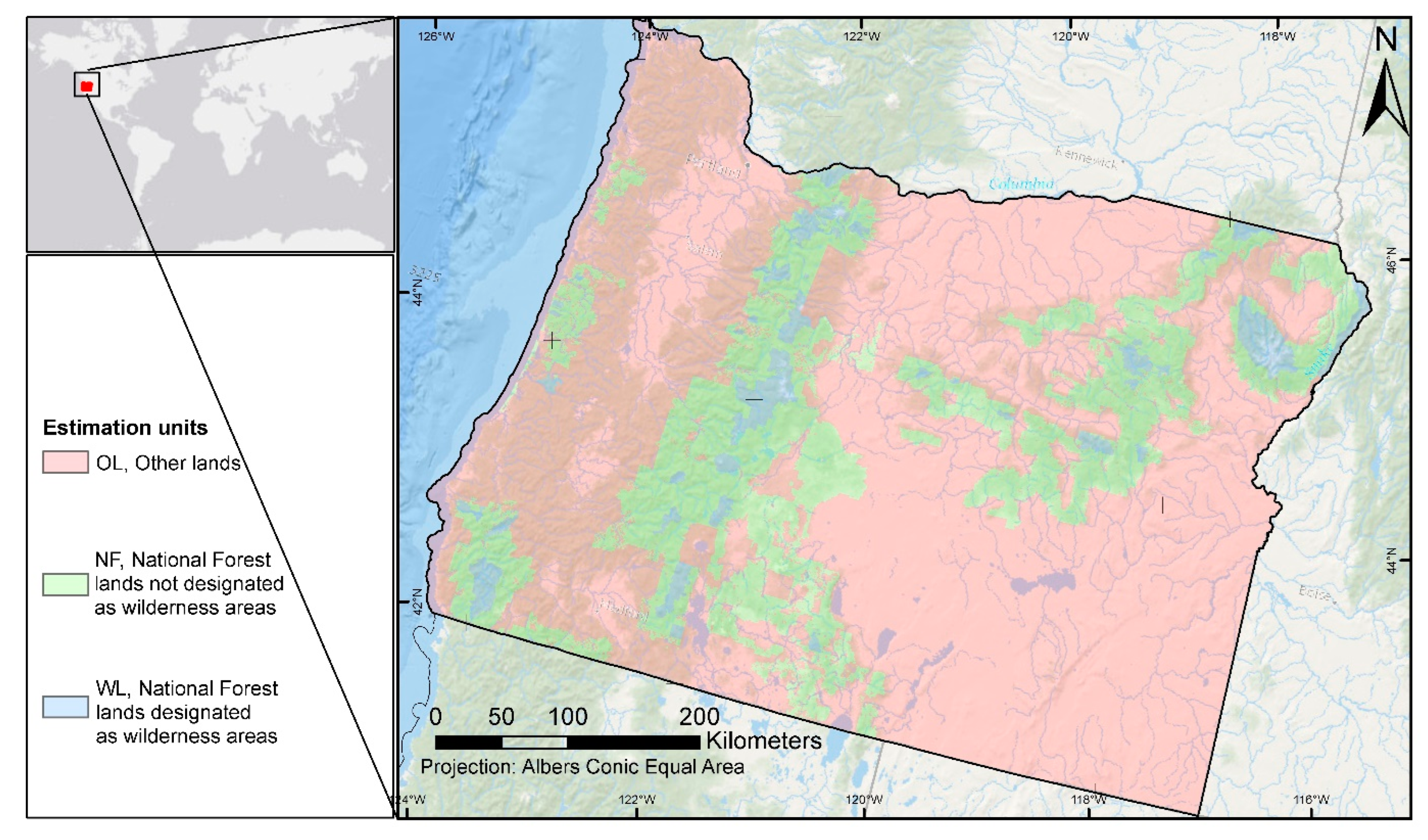
2.1. Study Area

This study was developed using the US state of Oregon as a testing area (Figure 1). Oregon is included in the PNW-FIA region, and its size, geographic position, and diversity make it well-suited for testing purposes. Oregon is 247,963 Km2 in size, and 48.4% is forested land, of which 64% is publicly owned [15]. Oregon has very strong west-to-east environmental gradients. The area west of the Cascade Range is moist and mild, with forest dominated by Douglas-fir, Pseudostuga menziesii (Mirbel) Franco, red alder, Alnus rubra Bong, western hemlock and Tsuga heterophylla (Raf.) Sarg. Areas east of the Cascade Range have a dry, continental climate, and the forests are dominated by ponderosa pine, Pinus ponderosa Lawson & C. Lawson, lodgepole pine, Pinus contorta Douglas ex Loudon, and western juniper, Juniperus occidentalis Hook.

2.2. Auxiliary Information

After the initial literature review, we compiled a set of auxiliary variables available for the PNW-FIA region that were potentially correlated with Δ A G B . This database contained proxies for potential forest AGB productivity, disturbances and AGB removals, and forest management regimes. All auxiliary variables were rasterized using a common 30 × 30 m grid using the NAD83 2011 reference system with conic Albers equal area projection to ensure that pixel counts can be directly translated to areas. Auxiliary variables contained variables considered static (i.e., did not change over time) and variables considered dynamic. For example, all proxies for potential AGB productivity, such as climate or topographic position, are not expected to change substantially within the period considered in this study and, therefore, were considered static. Proxies for management regimes were based on ownership maps. Ownership can change over time; however, in our analyses, we only considered extensive ownership categories that are not expected to have major changes within the study period. Thus, ownership was also considered a static variable. Proxies for disturbance and AGB removals and the annual CMS AGB maps were all dynamic and their preprocessing focused on obtaining variables that referred to 10-year periods matching the PNW-FIA panel design. For auxiliary variables computed as changes in land cover maps and changes in the annual CMS AGB map, it was impossible to calculate values for some of the 10-year periods considered in the analysis. In those cases, we allowed small temporal mismatches of up to two years with respect to the 10-year cycle under consideration. Finally, some auxiliary variables were categorical, and some were continuous. In Supplementary S1 of the supplementary material, we describe in detail: (1) the processing steps necessary to include each dataset in the database, (2) the derived auxiliary variables, (3) their categorical/continuous nature, and (4) whether they were considered as static or dynamic variables. This information is summarized in Table 1.

2.3. Estimation Framework

2.3.1. Population

We considered a finite population approach for estimation purposes. For the 10-year period starting year t , the set of all 30 m × 30 m spatial pixels in the state of Oregon was considered as a finite population of interest, U . The base grid of the auxiliary information database is itself the sampling frame and does not change over time. Finally, pixels are considered population units and are indexed by i = 1 , 2 , N , where N is the total number of pixels for the state. For the 10-year period starting in year t , every population unit i (i.e., pixel) has an associated q-dimensional vector of auxiliary variables denoted as x i t = x i 1 t , x i 2 t , , x i q t t . This vector contains all auxiliary variables for the 10-year period starting in year t . Every unit i also has associated values Δ A G B for the period, but those changes are unknown except for the locations that were measured, according to the panel design, at the beginning and end of the period (see Section 2.3.3).

2.3.2. Target Parameter

PNW-FIA considers changes corresponding to 25 possible combinations of conditions at times t and t + 10 . Still, some of these combinations correspond to unsampled areas at time one, time two, or both times or to sampled areas outside of the reporting scope of PNW-FIA. We focused our analysis on changes in areas that were forest at times t and t + 10 . The response for a population unit i in the decade starting in year t is denoted in the remaining sections as Δ A G B i t and is the annualized forest change of AGB per unit area.
Δ A G B i t = 1 10 ( A G B i t + 10 A G B i t )
A G B i t and A G B i t + 10 represent the AGB for areas that are forest at years t and t + 10 in unit i divided by the unit’s area. For non-forested units A G B i t , A G B i t + 10 and Δ A G B i t equal zero.
We defined the target parameter for the 10-year period starting on year t as the mean of Δ A G B i t
Δ A G B ¯ t = 1 10 N i = 1 N A G B i t + 10 i = 1 N A G B i t = 1 N i = 1 N Δ A G B i t .
We expressed the target parameter as a mean value per year and unit area change; however, converting this value to totals only requires multiplying Δ A G B ¯ t by the state’s known area and by 10 years.
We also considered estimating running means covering the periods   t 0 to t 0 + 10 through t 0 + a to t 0 + a + 10 . The target parameter in the case of a running mean covering the periods t 0 to t 0 + 10 to t 0 + a to t 0 + a + 10 is
Δ A G B ¯ t 0 , t 0 + a = 1 a t = t 0 t = t 0 + a 1 N i = 1 N Δ A G B i t

2.3.3. PNW-FIA Sampling Design and Sample

The sampling design used by PNW-FIA combines the general 2402.62 ha [17,18] FIA hexagonal grid with a 10-year rotating panel [15]. The result is a near systematic sampling design where one-tenth of the plots covering the entire state (i.e., a panel) are measured every year. In the PNW-FIA region, the sampling design was intensified on all National Forest Lands that were not designated Wilderness areas. Additional locations were selected for areas subject to intensification, which resulted in a field plot density 3.2 times higher than in non-intensified areas subject to the standard FIA design. Each of these new locations was assigned to one panel. The assignment to panels was done using a method that preserved the spatial balance of the sample within the intensified areas and provided an approximately constant number of intensification locations per panel [19].
All locations were initially inspected using orthophotos and GIS layers, and only those locations for which there was very strong evidence that they did not sustain any forest, i.e., urban areas, open farmland, or desertic areas, were labeled as non-forest [18]. All the remaining locations (including disturbed areas that currently had no live trees) were visited and measured by field crews that established plots and monumented the plot center to facilitate subsequent re-measurements (see [18] for a description of FIA measurement protocols).
For stratification purposes, three areas called estimation units, EU, are defined for each state in the PNW region. These areas are National Forest lands not designated as wilderness areas, NF, National Forest lands designated as wilderness areas, WL, and other lands, OL (Figure 1). Stratifications in the PNW region are developed in a way that ensures that a given stratum can only be present in a single EU. A layer with the delineation of the EUs was included in the auxiliary information database, and all EPS were developed respecting the constraint that no stratum can be present in more than one EU.
We considered that field plots for which less than 75% of the plot area was measured in both the first and second rounds of measurements were missing data. In addition, we also excluded plots for which the second measurement year was not 10 years after the first one (Table 2). Plots in which the first and second measurements were respectively taken in years t and t + 10 form the sample, s t , for that 10-year period. Note that extreme cases include plots for which the first and second measurements can be close to 9 or 11 years apart (e.g., a lag between measurements close to 9 years occurs when the first measurement is taken at the end of year t the second measurement at the beginning of year t + 10 ). Moreover, note that, as indicated in Section 2.3.1, for many plots, the value of the response is zero because they are in non-forested areas. The sample for estimation of running means, Equation (3), is the union of all the samples for the periods considered in the running mean, i.e., s t 0 t 0 + a = U t = t 0 t = t 0 + a s t . Finally, we used the criteria in [4,20] and assigned each field plot measurement to the pixel that contained the center of the plot.

2.4. Development of Models for EPS

Estimators under consideration used assisting models for which the expected value of Δ A G B i t equals
E Δ A G B i t = β t t   f x i t = β t t   z i t ,
where: x i t , is the q dimensional vector that contains the auxiliary variables in the spatial database for unit i , z i t results from applying to x i t a function f that maps vectors from the auxiliary variables space to a space that contains p -dimensional indicator vectors z i t providing the stratum membership for each unit. All entries in z i t are zero except for the one corresponding to the stratum where unit i is assigned to z i t k (i.e., the k t h entry of z i t , equals 1 if unit i belongs to the k t h stratum during the period starting year t and zero otherwise). The dimension p provides the number of strata and varies depending on the EPS estimator. The term β t is a vector of coefficients, and super index t is the transpose operator. Both f and β t need to be determined. The function f is linked to the type of EPS, and model coefficients β t need to be estimated using the sample data. Finally, for the assisting models, the variance of Δ A G B i t is a constant for each stratum k
V Δ A G B i t = σ k 2 ,   i f   i   s t r a t u m   k

2.4.1. General Model Selection Considerations

The number of variables in the auxiliary information database is large, and model selection steps were necessary to identify the function f used in each model-assisted estimator. All model selection steps were carried out to ensure that the final strata did not cut across EUs. Plots in areas classified as open-water, NLCD code 11, in all the NLCD land-cover maps were excluded from the model selection stage (Table 2). Model selection steps differed between estimators, and specific details for each estimator are provided in Section 2.4.2, Section 2.4.3, Section 2.4.4. Common steps related to the model selection processes were:
First, all model selection steps were done with the datasets that combined the eight 10-year periods under consideration. This allowed identifying unique models for all 10-year periods. All 10-year periods were represented in approximately equal proportions in the combined datasets used for model selection, ensuring that no 10-year interval received more weight than the others.
Second, the model selection steps were only used to identify f and the variables included in each assisting model. For a given 10-year period, final model coefficients were estimated using the field sample corresponding to the panel for the period under consideration, and for multiple 10-year periods, coefficients were estimated using the field sample of the corresponding panels.

2.4.2. GREG-EPS

In GREG-EPS, f uses dummy variables resulting from the interaction of E C O , O W N , C A T P C P I , C A T A C D I S T t , M A X F S E V t , and Δ N L C D t . There were 4700 combinations of values of these variables, and most combinations had such a small areal representation that they could not be directly considered potential strata. These interactions were collapsed into groups with an average area for which the expected number of plots per year was four or more. For each EU, the original combinations of categorical variables were collapsed using an algorithm that:
  • First, arranged all combinations on a tree that was constructed using the variables C A T A C D I S T t , E C O and O W N . Branches in the first level of the tree were defined using C A T A C D I S T t , and branches for the second and third levels were based on E C O and O W N , respectively. Each combination of E C O ,   O W N ,   C A T P C P I , C A T A C D I S T t , C A T P C P I , M A X F S E V t , and Δ N L C D t , resulted in a leaf that was placed in its corresponding branch depending on C A T A C D I S T t , E C O and O W N .
  • Leaves with four plots per year or more were set as fixed leaves. The remaining leaves were merged with other leaves (fixed or not) in the same branch. The merging process ran separately in each branch and started with the leaf with a smaller area in the branch. The selected leaf was merged with the closest leaf in the same branch. The Gower distance [21], computed with all categorical variables, was used to determine which leaf was the closest to the selected leaf. This distance was selected because it allows treating differently categorical variables with an implicit ordering (i.e., all categorical variables derived from a continuous one) and categorical variables without an implicit ordering (e.g., O W N ) . The two leaves were merged into a single leaf, and the expected number of plots per year was recomputed based on the area of the group resulting from the merge. If the expected number of plots per year of the resulting leaf was four or more, or if the small leaf was merged to a fixed leaf, the result was tagged as fixed, and it was not considered as a target for further merging steps.
  • Step 2 was repeated until all the resulting leaves in a branch had an expected number of four plots per year or all leaves in one branch were merged into a single leaf.
  • When merging all leaves in one branch did not yield an area from which to expect four plots per year, the merging process continued but considered merging groups from branches of the previous level of the tree (i.e., the algorithm continued with branches defined by C A T A C D I S T t and E C O first, and then with branches defined by C A T A C D I S T t only).
This collapsing procedure is analogous to the one used by FIA for PS. Its result was a set of 223 groups, and each of those groups was a potential post-stratum. The number of potential post-strata was still large, and we used the elastic net implementation from the R package glmnet [22] to determine which ones could be considered as final strata. Groups with non-zero coefficients were considered as final strata, and groups with zero coefficients were assigned to selected strata by first tagging the former as fixed and then applying steps 1 to 4 to the groups with zero coefficients but setting an area threshold larger than the state’s area to ensure that groups with zero coefficients were merged to groups with non-zero coefficients. The resulting groups formed the final set of post-strata, and each pixel of the auxiliary information database was assigned to its corresponding group. This resulted in the final PS maps for GREG-EPS.
It is important to note that the combinations of auxiliary variables that give rise to strata are defined using dynamic variables that change over time. To compute the expected sample size per year, we used the average area of each combination of categorical variables over the 8 periods considered in this analysis. This implies that the possibility of having unsampled strata for a particular 10-year period is significantly reduced but not eliminated. After testing with different area thresholds, an average expected sample size of four plots per year was selected, as it maintained the area of the unsampled micro-strata below 2.5% of the total area.
To assess the improvement in the estimation of Δ A G B when the auxiliary variables included the multiyear remote sensing CMS AGB map from [8], we repeated this process, adding C A T Δ C M S t to the pool of auxiliary variables. The branches of the tree for the collapsing process were defined with the same variables ( C A T A C D I S T t , E C O and O W N ). The elastic net model selection, final collapsing and strata mapping steps were repeated, and the result was an alternative EPS. We will refer to this EPS as GREG-EPS-CMS.

2.4.3. GL-EPS

The GL-EPS estimator proposed by Breidt and Opsomer [11] is developed based on a response that is selected as a PS variable. In our case, the PS variable is Δ A G B i t itself. A set of intervals is defined a-priori by the modeler on the range of the PS variable, and each one of those intervals will result in a final post-stratum. For example, an over-simplified set of intervals for Δ A G B i t could be , 0 and 0 , , i.e., losses and gains of forest AGB. Once the intervals for the PS variable are defined, GL-EPS estimators are obtained assuming that the PS variable can be predicted using a function, h , of a linear combination, γ t x t i , of the auxiliary information available
Δ A G B ^ i t = h γ ^ t x i t
The function h only needs to be a strictly monotone function [11] to ensure consistency of the GL-EPS estimator, which allows for very flexible specifications of h . In our study, we considered the simplest case and h was the identity function. To form the linear predictor, we considered all the categorical variables that were not derived from a continuous one (e.g., C A T P C P I was not considered because it was derived from the continuous variable P C P I ), all continuous variables, and all their pairwise interactions. The total number of variables and pairwise interactions present in the sample was 279. A model selection step was performed using the elastic-net regularization criteria [4] to reduce the number of coefficients in the linear predictor.
The intervals for Δ A G B i t were defined using the values reported for this variable by [16] in Panther Creek, western Oregon. This study provides a good reference for large values of AGB growth because the study site is located in one of the most productive areas of the state. Thresholds were defined using the following criteria:
  • The maximum value of Δ A G B i t reported by [16] was 8.75 Mg ha−1 year−1. Based on this value, we defined the following five positive intervals 0 , 2 ,   2 , 4 , 4 , 6   6 , 8 , and 8 , .
  • For disturbances causing losses in forest AGB with magnitudes comparable to growth, we used the thresholds used for growth but with negative signs. The last interval ( , 8 accommodates large and negative values of Δ A G B i t occurring after stand-replacing disturbances such as clear cuts.
Once models were selected, the non-zero coefficients γ ^ t were used to obtain predictions Δ A G B i t ^ for each population unit. These predictions were reclassified according to the defined threshold to obtain the corresponding stratum membership vectors z i t associated with each population unit and 10-year period. The model selection and mapping of strata was repeated, including Δ C M S t in the pool of auxiliary variables. We will refer to the EPS using Δ C M S t as GL-EPS-CMS.

2.4.4. TREE-EPS

For TREE-EPS, we applied the method proposed by McConville and Toth [14]. One partitioning tree was identified in the model selection stage for each EU. These trees were found using the rpms R package [23] that implements the partitioning algorithm described in [24]. All auxiliary variables, except Δ C M S t and those categorical variables derived from a continuous one, were used to find partitioning trees for each EU. Trees were used for each 10-year period to assign pixels and field plots to strata. This process was repeated including Δ C M S t in the pool of auxiliary variables to assess the improvement in the estimation of forest AGB derived from the use of this auxiliary variable. We will refer to the EPS based on tree models using Δ C M S t as TREE-EPS-CMS.

2.5. Estimators of Δ A G B and Variance Estimators

The three EPS variants were compared to the exogenous PS estimators currently used by PNW-FIA, FIA-PS, hereafter, and to the well-known HT estimator. As target parameters, we considered means and running means of forest AGB. Estimators are described in detail for the base case where the target parameter is the mean Δ A G B for a single 10-year period. For running means, we present the modifications with respect to the base case that is needed. For both single 10-year periods or running means of more than one 10-year period, the possibility of having unsampled strata exists. This can cause differences in the areas used to make comparisons between methods. In order to overcome this problem, the presence of unsampled strata was addressed by merging all unsampled strata in a given EU to the sampled strata with the largest area in the EU.

2.5.1. Approximation to Sampling Design Weights and Point and Variance Estimators

All estimators under consideration are design-based estimators. Their expressions and associated variance estimators require knowing first and second-order inclusion probabilities. Due to many factors, such as denial of access or hazardous plot locations, the number of plots measured in the field does not match that planned in the design. In order to account for this fact, inclusion probabilities are empirically adjusted based on the sample size and the total number of pixels in the stratum of the plot. This adjustment implies the assumption that plots are missing at random within strata. For plot i measured in the period t to t + 10 in stratum k , the adjusted inclusion probability used in the further analysis was
π i t = n t   k N k     ,
where n t k and N k are the number of plots and pixels in the stratum that contains i . When estimating running means, the sample size and number of pixels within each stratum were the sum of the sample sizes and the number of pixels for the periods considered in the running mean.
We assumed that the selection of FIA plots happened independently and computed pairwise inclusion probabilities for two elements, i j in the sample as
π i j t = π i t π j t
When i = j then π i i t = π i t . The total number of FIA plots, and the number of intensification plots for each 10-year period are provided in Table 2.

2.5.2. Point and Variance Estimators

PS and EPS estimators are obtained from the general formula for a GREG estimator
Δ A G B ¯ ^ t = 1 N i = 1 N β ^ t t z i t + 1 N i s t Δ A G B i t β ^ t t   z i t π i t   ,
The first summand in Equation (9) provides the mean value of Δ A G B predicted by the assisting model and the second summand is a bias correction factor that accounts for possible misspecifications of the assisting model. For PS and EPS models verifying Equations (4) and (5), the second summand equals zero, and the estimator of Δ A G B for the state can be simplified to
Δ A G B ¯ ^ t = k = 1 p W k t β ^ k t
where W k t = N k t N is the k t h stratum weight, with N k t the number of units in the population mapped by f to stratum k in the considered period. The coefficients β ^ k t are the Hajek estimators of the stratum means of Δ A G B for the decade extending from year t to year t + 10 .
β ^ k t = Δ A G B ^ k t N ^ k t .
The numerator in Equation (11) is
Δ A G B ^ k t = i s t Δ A G B i t π i t z i k t ,
the HT estimator of the total Δ A G B for the 10-year period in the k t h stratum. The denominator of Equation (11) is
N ^ k t = i s t 1 π i t z i k t
is the HT estimator of the stratum size.
A Taylor approximation for the variance of the estimator in Equation (10) is
V Δ A G B ¯ ^ t = 1 N 2 i U j U Δ i j t e i t 0 e j t 0 π i t π j t
where e i t 0 = Δ A G B i t β ^ 0 t t z i t , and β ^ 0 t t z i t is the prediction of Δ A G B i t if the assisting model was fit using the data for the entire population [7] p. 237. The variance in Equation (14) can be estimated using the variance estimator
V ^ Δ A G B ¯ ^ t = 1 N 2 i ϵ s t j ϵ s t π i j t π i t π j t π i j t g i t e i t π i t g j t e j t π j t
where e i t = Δ A G B i t β ^ t t z i t and g i t = N g t N ^ g t [7] p. 264. From Equation (8), we obtain π i j t π i t π j t = 0 , if i j and Equation (15) reduces to:
V ^ Δ A G B ¯ ^ t = 1 N 2 i ϵ s t 1 π i t N k t e i t N ^ k t π i t 2
Estimates of the running mean for the periods t 0 to t 0 + 10 through t 0 + a to t 0 + a + 10 and their associated variances were obtained by extending the sums in Equations (12), (13), (16), (17), and (18) to the elements of s t 0 t 0 + a and replacing N by a N .

2.5.3. Comparison to Current PNW-FIA Estimators and Horvitz-Thompson Estimators

Improvements in precision with respect to the current PNW-FIA practices were assessed by comparing the EPS estimators developed in this study to those resulting from FIA-PS. PS and EPS estimators differ in how the post-strata are obtained, but once the post-strata are created, Formulas (9) though (18) are used for both types of stratifications. To analyze improvements in precision with respect to a situation in which no auxiliary information is available, we compared the developed EPS estimators and FIA-PS estimators to the HT estimator
Δ A G B ¯ ^ π t = 1 N i s t Δ A G B i t π i t
In this case, no strata were used, and adjustments of inclusion probabilities were performed at the EU level. Thus, π i t were computed as π i t = n t   E U N E U with N E U and n t   E U the number of pixels and sample size in the EU where unit i is located. The variance of the HT estimator was computed as
V ^ Δ A G B ¯ ^ π t = 1 N 2 i ϵ s t 1 π i t Δ A G B i t π i t 2
For a given PS or EPS estimator, M , where M can be GREG-EPS, GREG-EPS-CMS, GL-EPS, GL-EPS-CMS, TREE-EPS, TREE-EPS-CMS and FIA-PS, the relative efficiency for the period starting year t was computed as
Δ V ^ M t = 1 V ^ Δ A G B ¯ ^ M t V ^ Δ A G B ¯ ^ π t
This metric provides an estimate of the reduction in the variance that the estimator M produces with respect to the HT estimator in terms relative to the variance of the latter. Comparisons with FIA-PS were analyzed by observing the differences between Δ V ^ M t   and Δ V ^ F I A P S t .

3. Results

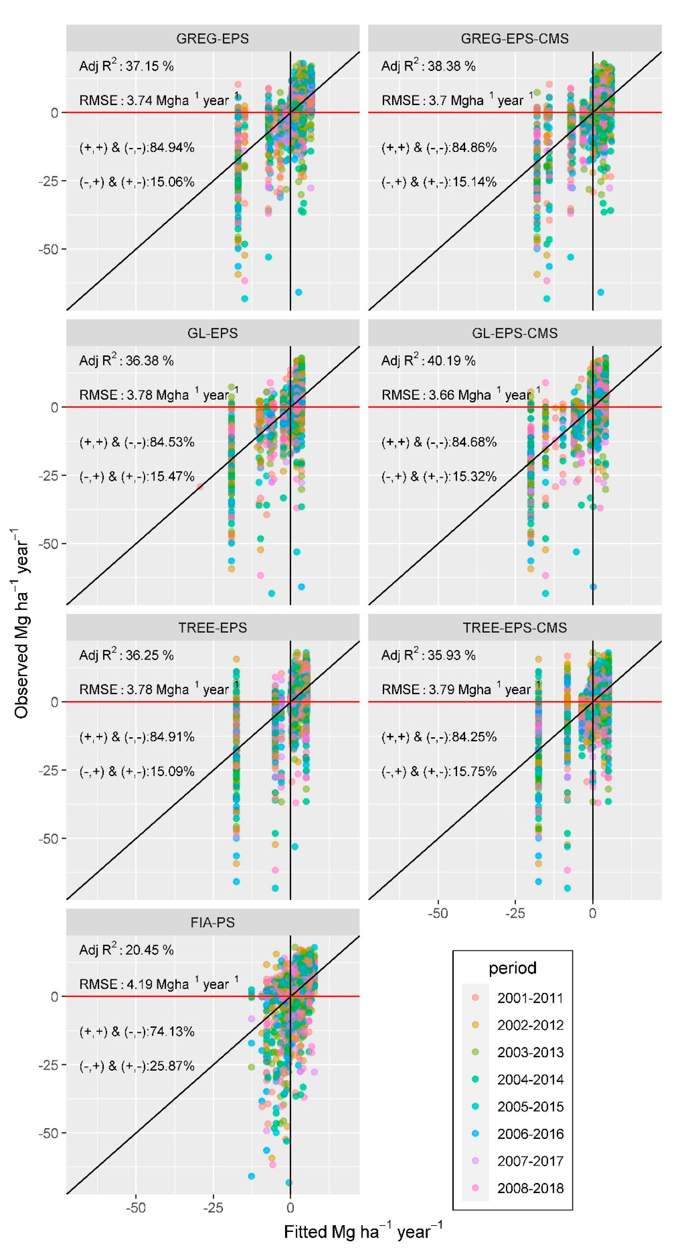
3.1. EPS and PS Assisting Models and Summaries

The most important differences between EPS methods and FIA-PS were that EPS methods tended to explain a larger amount of the variance of Δ A G B , but created a smaller number of strata (Figure 2). Adjusted coefficients of determination, Adj-R2, for the assisting models for EPS methods ranged between 35.93% to 40.19%, while R2 for FIA-PS was 20.45%. Root mean squared errors, RMSE, for the assisting models ranged from 3.66 Mg ha−1 year−1 to 3.19 Mg ha−1 year−1 for EPS methods, while RMSE for FIA-PS was 4.19 Mg ha−1 year−1. The proportion of plots with observed and predicted values of Δ A G B with the same sign (i.e., positive changes predicted as positive and negative changes predicted as negative changes) ranged from 84.25% to 84.94% for EPS methods. For FIA-PS, this percentage was 74.13%. These results indicate that the EPS variants analyzed in this study can improve the precision of the current estimates of Δ A G B . GL-EPS was the method that experienced the largest improvements in terms of Adj-R2 when Δ C M S t was added to the stack of auxiliary variables, Adj-R2 was 36.38% for GL-EPS and 40.19% for GL-EPS CMS. Adding Δ C M S t to the pool of auxiliary variables had a minor effect on GREG-EPS (i.e., Adj-R2 was 37.15% for GREG-EPS and 38.38% for GREG-EPS-CMS). The model for TREE-EPS had an Adj-R2 of 36.25% and explained slightly more variance than the model for TREE-EPS-CMS, with an Adj-R2 of 35.93%.
Assisting models for EPS methods were substantially more parsimonious than the region’s current PS. The EPS model with the most strata was the model for GREG-EPS-CMS. This model created 97 strata, approximately one-half of the number of strata of FIA-PS (Table 3). The most important similarities between the spatial representation of the EPS developed in this study were that: (1) strata close to the coast, and Willamette valley were the ones that had larger and positive stratum means, (2) strata with large negative changes appeared scattered on the western third of the state (west of the cascades mountains) where most intense industrial forest practices occur and (3) the eastern side of the state was characterized by stratum means that were close to zero, with the exception of the areas on the Ochoco National Forest and the Blue and Wallowa mountains located in northeast Oregon. The most important differences between EPS methods are derived from the number of strata they generated (Table 3). GREG-EPS and GREG-EPS-CMS were the methods that resulted in more strata, and associated strata maps provided a finer-grained representation of the variability of Δ A G B (Figure 3). GL-EPS and GL-EPS-CMS were the most parsimonious EPS models, and the resulting strata maps captured large-scale trends but showed low variability at local scales (Figure 3). Finally, TREE-EPS and TREE-EPS-CMS resulted in stratifications with an intermediate level of detail (Figure 3).
EPS models used both static and dynamic auxiliary variables. The collapsing steps for GREG-EPS and GREG-EPS-CMS were driven by the variables C A T A C D I S T t , E C O and O W N . However, these variables alone do not justify the final number of strata which indicates that other variables play a role in the stratification. The model for GL-EPS used the variables E L E V and P C P I , A C D I S T t and Δ N L C D t , and the model for GL-EP-CMS used E L E V , P C P I , A C D I S T t and Δ C M S t . All variables except M A X F S E V t , were used to form at least one node of the partitioning tree of TREE-EPS, but the variables Δ N L C D t and A C D I S T t determined the majority of the splits. For TREE-EPS-CMS, all variables except A C D I S T t and M A X F S E V t appeared in at least one split of the partitioning tree (see supplementary material Supplementary S2). Δ C M S t and Δ N L C D t determined most of the splits in the binary tree with Δ C M S t playing a role such as that played by A C D I S T t in TREE-EPS. The partitioning tree for EU WL was the same for TREE-EPS and TREE-EPS-CMS. The only variable that was never used in the models for TREE-EPS, TREE-EPS-CMS, GL-EPS or GL-EPS-CMS was M A X F S E V t which indicates that it provides information that is redundant with A C D I S T t and Δ C M S t , the other auxiliary variables derived from spectral data from Landsat images.
GREG-EPS, GREG-EPS-CMS, GL-EPS, GL-EPS-CMS, and FIA-PS resulted in micro-strata with a minimal presence in the territory and that were not sampled. This problem was most relevant for FIA-PS, where the proportion of area corresponding to unsampled strata ranged from 2.3% to 4.6% (Table 3). The collapsing process minimized but did not eliminate the problem of creating empty strata for GREG-EPS and GREG-EPS-CMS, where the area of the unsampled strata reached 0.2% and 0.9%, respectively (Table 3). For GL-EPS and GL-EPS-CMS, unsampled strata appeared in all EUs. Their area representation was less than 0.6% and 0.9% of the total area, respectively (Table 3). The recursive partitioning algorithm of TREE-EPS avoids creating empty strata and incorporates a tuning parameter that ensures that strata have a minimum sample size specified by the modeler. A minimal fraction of area corresponding with no-data values in some of the auxiliary variables used for TREE-EPS and TREE-EPS-CMS resulted in areas without stratum assignments. However, the proportion of those areas was less than 0.001% of the total area (Table 3). The areal extent of the unsampled strata decreased when considering multiple periods for running means. All strata were sampled for all methods except GL-EPS and GL-EPS-CMS when considering the eight periods combined. For GL-EPS and GL-EPS-CMS, the area that the unsampled strata represented in the territory was reduced to less than 0.05%.

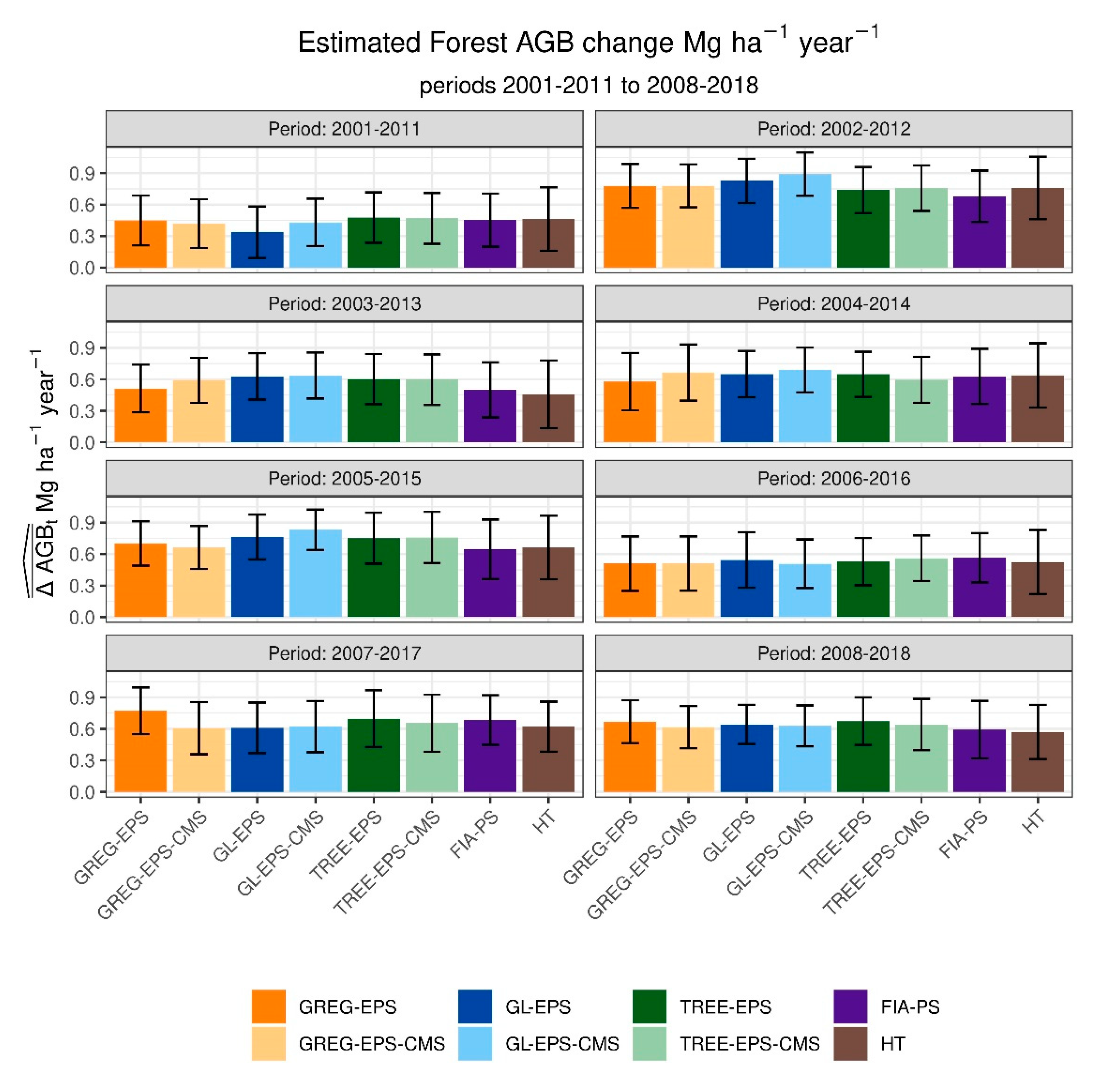
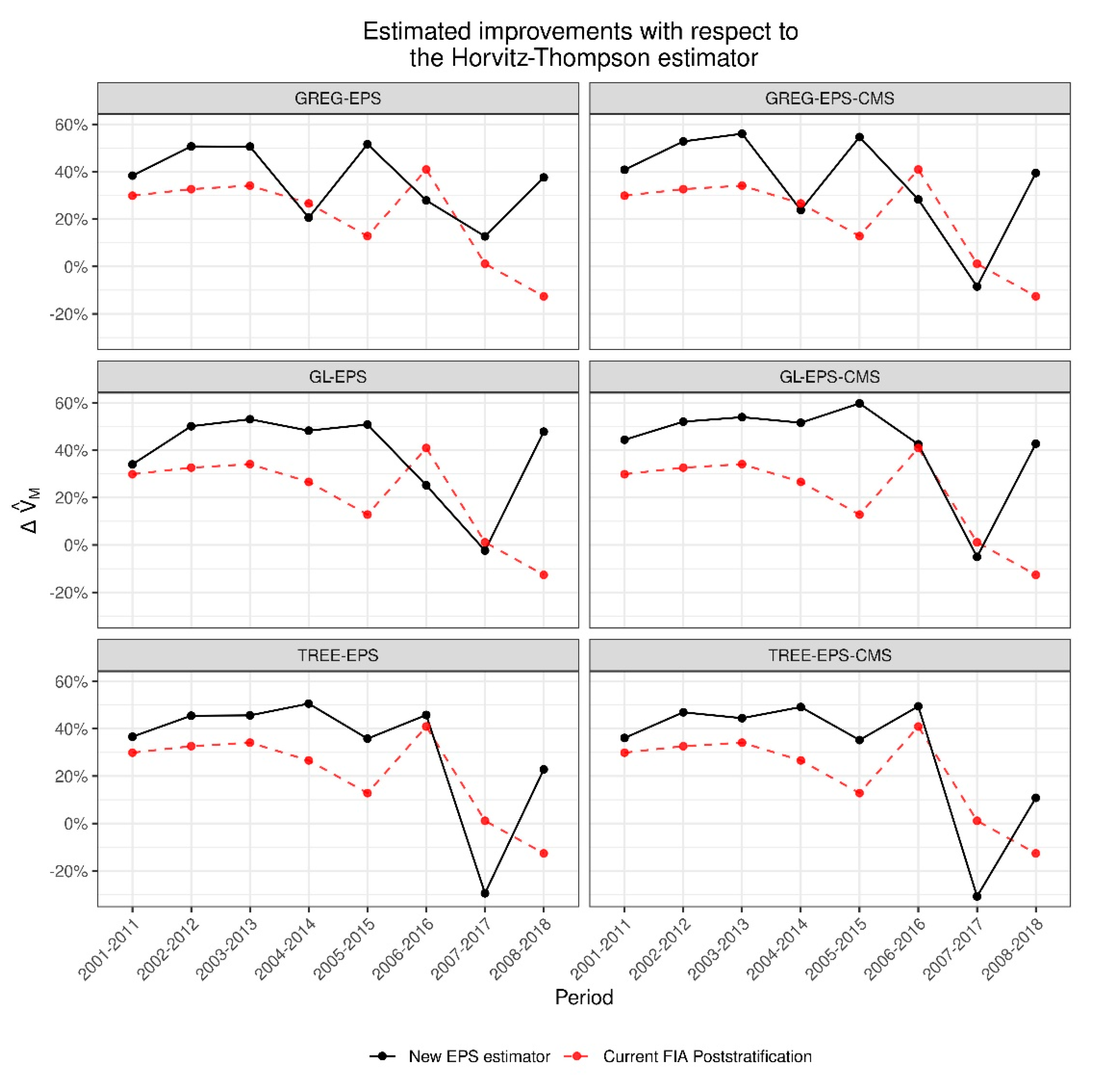
3.2. Estimates of Changes for the State for Specific 10-Year Periods

All methods, including the HT estimator and the FIA-PS, estimated that total Δ A G B (per unit area and year) for all periods under consideration was positive (Figure 4). This clearly indicates a steady increase in forest AGB in the region. Estimated change ranged from 0.33 Mg ha−1 year−1 to 0.88 Mg ha−1 year−1 depending on the 10-year period and estimator. Differences between estimated totals for different periods tended to be of larger magnitude than differences between methods for a given period (Figure 4).
Estimated improvements in precision with respect to the HT estimator, Δ V ^ M , varied across model-assisted estimators and also across periods; however, some general trends were observed. All model-assisted estimators, including the PS currently used by PNW-FIA, consistently improved the precision of the HT estimator (Figure 5). The only exception to this trend was 2007–2017 for all EPS variants except for GREG-EPS and the periods 2007–2017 and 2008–2018 for FIA-PS. The low value of Δ V ^ M for 2007–2017 that was obtained for all EPS methods and FIA-PS is due to an unusually low variance of the HT estimator for this period.
The median improvement obtained by the EPS and PS estimators with respect to the HT estimator indicated that GL-EPS-CMS and GL-EPS produced larger gains in precision than other EPS methods. The median improvement for GL-EPS-CMS and GL-EPS was 48.02% and 47.99%. These methods were followed by GREG-EPS-CMS and GREG-EPS, TREE-EPS-CMS, and TREE-EPS, with improvements in the efficiency of around 40%. FIA-PS produced a median improvement with respect to the HT estimator of 28.24%. EPS variants were generally more efficient than FIA-PS (Table 4), but FIA-PS outperformed EPS methods in at least one of the 10-year periods (Figure 5).

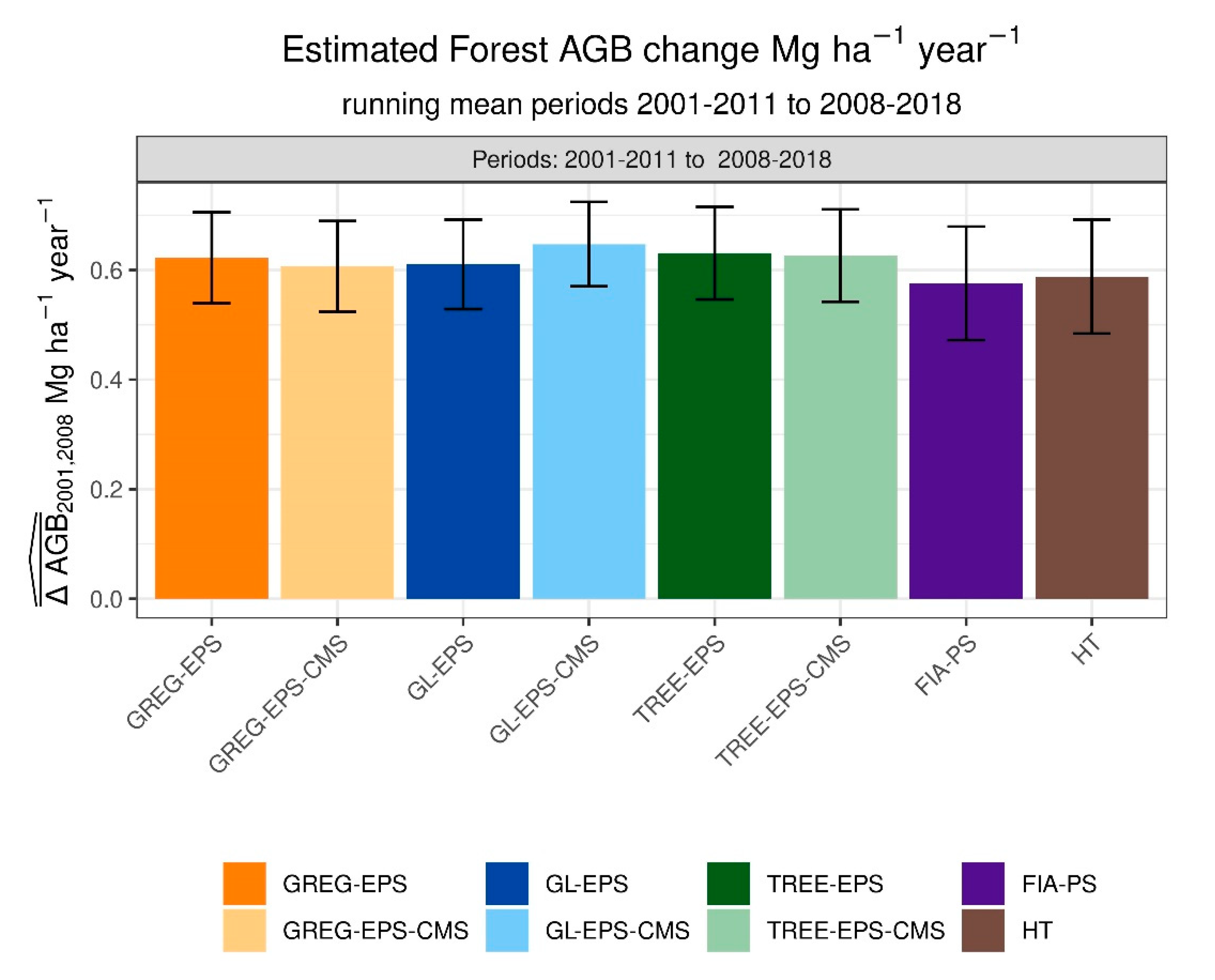
3.3. Estimators of Running Means

When considering running means of more than one 10-year period, the patterns we observed were similar to those observed for single 10-year periods (Figure 6). All methods consistently estimated positive values of Δ A G B and EPS methods and FIA-PS resulted in gains in performance with respect to the HT estimator. With only a few exceptions, EPS methods also resulted in gains in performance with respect to FIA-PS (Figure 6). As expected, when increasing the number of 10-year periods included in the running means, differences between the estimates and associated uncertainties provided by the tested methods decreased at a rate that was approximately inversely proportional to the square root of the combined sample size. Running means for the eight 10-year periods ranged between 0.58 Mg ha−1 year−1 and 0.65 Mg ha−1 year−1, and confidence intervals for the estimates provided by any method contained the estimates provided by the other methods (Figure 7). For the running means of eight 10-year periods, adding Δ C M S t to the pool of auxiliary variables consistently resulted in values of Δ V ^ M larger than those obtained by EPS models not using this auxiliary variable. Differences between GL-EPS and GL-EPS-CMS were largest at 6.7%, i.e., 38.3% vs. 45.0%, and differences between GREG-EPS and GREG-EPS-CMS and TREE-EPS and TREE-EPS-CMS were of small magnitude < 1%, i.e., 36.1% vs. 36.23% and 33.95 vs. 34.2%, respectively.

4. Discussion

4.1. Similarities between Model-Assisted Estimators

All methods estimated increases in forest AGB for the periods 2001–2011 to 2008–2018 (Figure 4). This indicates that despite increasing large-scale wildland fires and insect outbreaks (i.e., bark beetle) events over the last two decades, there is a net accumulation of forest AGB in the region. Depending on the method, the average estimated change over the eight 10--year periods analyzed in this study ranged between 0.58 Mg ha−1 year−1 and 0.65 Mg ha−1 year−1. These results indicate a consistent increase in forest AGB in the study area but do not inform about the type of changes that are occurring. The accumulation of forest AGB can result from many processes of a very different nature and with very different ecological implications. For example, both: (1) increases in the amount of land sustaining mature forest structures with larger trees and more fire resilient structures, and (2) increases in the amount of young and dense forest structures resulting from fire suppression efforts contribute to total forest AGB accumulation. The ecological implications of each type of increase mentioned above are very different and could be evaluated by a more detailed analysis of the field-measured plot data. However, PS and EPS allow constructing additive tables for non-overlapping categories in a straightforward manner. Thus, these methods can be used to derive estimates of change by typologies.
EPS estimators developed in this study use a method closely related to the direct approach proposed by McRoberts et al. (2015) because Δ A G B is the modeled variable. However, small differences with the direct approach exist due to the inclusion of static auxiliary variables. Estimators developed in this study or using direct approaches [20,25,26,27] are typically preferred over indirect methods where assisting models are developed for A G B and then estimates for time 2 and time 1 are differenced. Direct methods offer a more straightforward way of modeling change; however, because a different response is modeled and different auxiliary variables are used, the estimated changes from a direct estimator would not match the difference between the AGB totals for time 2 minus those for time 1 of an indirect estimator.

4.2. Model Selection

Models were selected with a dataset that combined all the 10-year periods under consideration. Once models were selected, they were re-fitted with the data for a specific 10-year interval or intervals in the case of running means. This implies trade-offs between consistency, performance, and operationality, which can be summarized in the following remarks. Identifying unique models for all 10-year periods combined is operationally simpler than developing models for each period separately, but the resulting models are not necessarily optimal for any particular 10-year interval. Although this lack of optimality can certainly occur, all model-assisted estimators outperformed the HT and the PS estimators currently used by PNW-FIA. When the model selection is developed with the combined sample of eight 10-year periods, estimating Δ A G B for a specific 10-year interval is similar to obtaining estimates for a subpopulation of a larger one, the one resulting from the union of the populations of the eight 10-year periods. Differences in the relationships between auxiliary variables and Δ A G B are not expected to vary substantially across periods, and obtaining stratum-specific means and variances for each 10-year period separately should minimize potential bias problems.

4.3. Differences between Model-Assisted Estimators

In terms of performance, EPS methods exceed the HT estimator and FIA-PS. The development of a model-assisted estimator for an NFI implies evaluating the estimator’s performance but also several factors related to their practical implementation. We found that differences in performance between EPS methods were small and decreased when considering running means. Thus, we envision that operational constraints will likely outweigh performance considerations when selecting an EPS method to produce official stratification tables. One factor that we found especially challenging for the development of EPS was that the chances of finding micro-strata that need to be collapsed increased very rapidly when adding auxiliary variables. Model selection methods such as elastic net facilitated EPS development and reduced the need for strata-collapsing processes. However, the application of these methods, except for TREE-EPS, was far from being completely automatic.
For GREG-EPS, directly performing a model selection step on a saturated model, including all categorical variables and their interactions, produced a very large number of strata, many of them with a very small or zero sample size. It was necessary to perform an initial pre-collapsing stage that grouped similar interactions. These groups were considered in the elastic-net selection procedure, and the resulting models required a final collapsing of groups discarded by the elastic-net method. The need for collapsing steps for this method can be considered its main disadvantage. The way in which categorial variables are defined (i.e., the number of categories per variable) and the number of auxiliary variables need to be carefully considered as the number of initial groups that need to be collapsed grows very quickly. This task involves decisions by the modeler and involves some degree of subjectivity. In addition, a direct consequence of the need for a collapsing step is that interpretability of the generated strata is less straightforward than for TREE-EPS or GL-EPS. After the collapsing process, strata can be interpreted as groups of pixels with similar auxiliary information. Still, these groups are likely to have some internal variability, and producing a full description of the strata requires backtracking a large number of initial combinations of categorical variables that were merged during the collapsing process.
The definition of strata for GL-EPS is relatively straightforward, and the strata themselves have a meaningful interpretation, which is an advantage of this method. An important difficulty of GL-EPS was finding meaningful thresholds of the variable of interest that ensured that no empty strata were created. This problem was discussed by [12] and is accentuated when strata are forced to belong to only one EU. We used broad categories of Δ A G B , and still some strata were unsampled for specific 10-year periods. The areal representation of unsampled strata was small, below 1% in all considered periods, but remained even when considering the running mean of all the 10-year periods (Table 3). Unsampled strata tended to correspond with the extreme intervals defined for Δ A G B and could be merged to the neighboring strata. However, this solution implies that the final thresholds that give rise to the final strata are not defined a priori, which is the case considered in the definition of GL-EPS [11].
The simple GL-EPS version used in this study uses the identity function for h , which explains why observed improvements in performance when adding Δ C M S t were larger for this method than for the other EPS variants. Using the identity function for h makes GL-EPS utterly reliant on the linear predictor γ t t x t i . The auxiliary variable Δ C M S t was computed from validated AGB predictions and its association with Δ A G B improves the linear predictor. Other EPS variants experienced small or negligible improvements when using Δ C M S t . Because of their greater ability to model nonlinear relationships, they were able to find associations in the auxiliary information database that explained most of the variability explained by Δ C M S t . The design consistency of EPS estimators, similar to GL-EPS in their construction, but using non-parametric models instead of a linear predictor γ t t x t i has been proven [12]. Further research must explore these non-parametric versions of GL-EPS estimators because more flexible model specifications will likely capture non-linear relationships between auxiliary information and Δ A G B . The simple specification used for GL-EPS is not necessary a disadvantage. The linear predictor provides pixel level predictions γ t t x t i of Δ A G B and this intermediate output is interesting on its own. It provides a 30 m resolution map of Δ A G B that can be used for multiple purposes, including the computation of GREG estimators similar to those in [6,20,28].
Finally, TREE-EPS clearly outperformed all other alternatives for PS when considering easiness of practical implementation. By design, the recursive partitioning algorithm from Toth and Eltinge (2011) ensured that no empty strata were created. The implementation of this method in the rpms R package [23] allows setting minimum sample sizes for the final strata, which allows for fine-tuning of the PS process and minimizes the chances of obtaining unsampled strata in specific 10-year intervals. Furthermore, TREE-EPS can model non-linear relationships, eliminating over-smoothing problems observed for GL-EPS. In addition, it easily accommodates large numbers of auxiliary variables of mixed type (i.e., continuous and categorical), and the assisting model itself is a binary classification tree with a straightforward interpretation (see supplementary material Supplementary S2).

4.4. Other Considerations of Practical Importance

4.4.1. Estimation of Variance and Estimation of Change for Periods Not Matching the PNW-FIA Panel Frequency

PNW-FIA, and most NFI globally, rely on systematic or near-systematic sampling designs that make it impossible to obtain unbiased variance estimators [29,30]. The standard procedure is to either treat systematic samples using formulas for simple random sampling or treat the elements in the sample as if they proceeded from independent draws, as we did in this study. Computing variances in any of these ways can lead to bias problems, especially when the response shows strong trends. A priori, this problem is less important for model-assisted estimators that explain a significant portion of the response variability because weaker trends should be present in the model residuals needed for variance estimation (e.g., Equation (15)). Nevertheless, the problem is not eliminated, and alternative variance estimators have been proposed to account for spatial correlations when estimating variances from systematic samples [31,32,33]. Recent studies have shown that using these estimators with FIA data can improve the efficiency when estimating variances of spatially correlated attributes, even after post-stratification [34].
Estimation of change for periods that do not match the panel cycle is another topic that deserves attention (e.g., estimation of changes for 3-year period). One feature of the rotating panel design of FIA is that panels do not overlap. This enforces the change estimation for lags that are not multiples of the rotating panel period to rely on differencing estimators of A G B totals for state at times 1 and 2. If A G B ¯ ^ t 1 , and A G B ¯ ^ t 2 are the estimators for the totals at time t1 and t2, with the difference between t1 and t2 not a multiple of the panel period, then the estimated change is Δ A G B ¯ ^ t 1 , t 2 = A G B ¯ ^ t 2 A G B ¯ ^ t 1 , and its variance is
V Δ A G B ¯ ^ t 1 , t 2 = V A G B ¯ ^ t 2 + V A G B ¯ ^ t 1 2 C o v A G B ¯ ^ t 2 ,   A G B ¯ ^ t 1
From Equation (20), one can clearly see that a way to obtain more reliable estimators of change for a lag that is not a multiple of the rotating panel period is to minimize V A G B ¯ ^ t 1 and V A G B ¯ ^ t 2 [35]. This can be achieved by applying the techniques that we used for Δ A G B to A G B : however, applying different models for different times can result in strata with cumbersome interpretations. Variance estimators for V Δ A G B ¯ ^ t 1 , t 2 involve assumptions similar to those previously discussed. In particular, the estimation of V A G B ¯ ^ t 1 and V A G B ¯ ^ t 2 are instances of the same problem, and the same unknowns and potential solutions apply to them. Methods to provide spatially balanced samples with a time overlap have been proposed [36] and could be used to estimate 2 C o v A G B ¯ ^ t 2 ,   A G B ¯ ^ t 1 . However, the implementation of those solutions would require prohibitively costly and deep modifications of the FIA sampling design.

4.4.2. Auxiliary Variables

Finally, one of the most time-consuming steps of this study was compiling a database with auxiliary variables potentially correlated with changes in forest AGB. This step was critical as model-assisted estimators’ performance improvements are directly related to the strength of the correlation between response and auxiliary variables. This study was developed using the state of Oregon as a relatively data-rich test area, but several questions regarding the development of a similar auxiliary information database need to be considered if similar estimators are to be developed in other regions. Static auxiliary variables such as climate normals or topographic indexes are not expected to change substantially over time, and suitable replacements exist for most of these datasets in other areas of the world. Dynamic auxiliary variables require more careful attention. The independence of Δ C M S t and C A T Δ C M S t of the FIA sampling design makes these datasets very appealing for FIA and can enhance estimates of biomass change or simplify model fitting processes. In general, dynamic auxiliary variables are expected to have increasing relevance in NFIs as new multitemporal datasets become available. Thus, the maintenance of these datasets will be a critical factor in ensuring that NFIs can derive official tables periodically.

5. Conclusions

The main conclusions of this study can be summarized as follows:
EPS methods allowed accommodating static and dynamic auxiliary variables and showed their potential to improve PS methods currently used in FIA for the estimation of Δ A G B .
All EPS methods had operational advantages and disadvantages, and issues related to implementation, generation of unsampled strata, or interpretability of the generated strata might outweigh performance considerations.
GL-EPS relied on the construction of a linear predictor and adding Δ C M S t to the pool of auxiliary variables produced substantial performance improvements. This indicates that Δ C M S t can help in the estimation of Δ A G B . TREE-EPS and GREG-EPS were able to model non-linear relationships that explained most of the variability explained by Δ C M S t .
Changes in Δ A G B in the study were always positive, even when considering running means of multiple 10-year periods. Estimated changes provide average values of change but do not inform about the nature and type of change. However, the generated strata correctly identified known features in the landscape, which indicates that these EPS can play an important role in studies disaggregating Δ A G B by typologies.

Supplementary Materials

The following supporting information can be downloaded at: https://www.mdpi.com/article/10.3390/rs14236024/s1, Supplementary S1. Construction of the auxiliary information spatial database [8,9,37,38,39,40,41,42,43,44,45,46,47,48,49,50]; Supplementary S2. Summary TREE-EPS and TREE-EPS-CMS.

Author Contributions

F.M., V.J.M., A.N.G., O.K. and H.T. conceived the analysis. F.M. performed the computations, data curation, and analysis and wrote the first version of the manuscript. A.T.H., P.A.F. and Z.Y., created and interpreted the auxiliary maps and critically reviewed the manuscript, and provided feedback. All authors have read and agreed to the published version of the manuscript.

Funding

This work was supported by the Joint Venture Agreement 18-JV-11261959-049 between Oregon State University and the USDA Forest Service Pacific Northwest Region and by a NASA Carbon Monitoring System Program award (80HQTR20T0002) through a Joint Venture Agreement (20-JV-11221633-112) between the USDA Forest Service Rocky Mountain Research Station and Oregon State University. This research was supported by the USDA Forest Service, Rocky Mountain Research Station. The findings and conclusions in this publication are those of the authors and should not be construed to represent any official USDA or U.S. Government determination or policy.

Conflicts of Interest

The authors declare that the research was conducted in the absence of any commercial or financial relationships that could be construed as a potential conflict of interest.

References

  1. Breidenbach, J.; Granhus, A.; Hylen, G.; Eriksen, R.; Astrup, R. A Century of National Forest Inventory in Norway–Informing Past, Present, and Future Decisions. For. Ecosyst. 2020, 7, 46. [Google Scholar] [CrossRef] [PubMed]
  2. Kovac, M.; Gasparini, P.; Notarangelo, M.; Rizzo, M.; Cañellas, I.; Fernández-de-Uña, L.; Alberdi, I. Towards a Set of National Forest Inventory Indicators to Be Used for Assessing the Conservation Status of the Habitats Directive Forest Habitat Types. J. Nat. Conserv. 2020, 53, 125747. [Google Scholar] [CrossRef]
  3. Tomppo, E.; Gschwantner, T.; Lawrence, M.; McRoberts, R.E.; Gabler, K.; Schadauer, K.; Vidal, C.; Lanz, A.; Ståhl, G.; Cienciala, E. National Forest Inventories. Pathw. Common Report. Eur. Sci. Found. 2010, 1, 541–553. [Google Scholar]
  4. McConville, K.S.; Moisen, G.G.; Frescino, T.S. A Tutorial on Model-Assisted Estimation with Application to Forest Inventory. Forests 2020, 11, 244. [Google Scholar] [CrossRef] [Green Version]
  5. Lawrence, M.; McRoberts, R.E.; Tomppo, E.; Gschwantner, T.; Gabler, K. Comparisons of National Forest Inventories. In National Forest Inventories; Springer: Berlin/Heidelberg, Germany, 2010; pp. 19–32. [Google Scholar]
  6. Breidenbach, J.; Astrup, R. Small Area Estimation of Forest Attributes in the Norwegian National Forest Inventory. Eur. J. For. Res. 2012, 131, 1255–1267. [Google Scholar] [CrossRef]
  7. Särndal, C.-E.; Swensson, B.; Wretman, J. Model Assisted Survey Sampling (Springer Series in Statistics); Springer Science & Business Media: Berlin/Heidelberg, Germany, 2003. [Google Scholar]
  8. Fekety, P.A.; Hudak, A.T. Annual Aboveground Biomass Maps for Forests in the Northwestern USA, 2000–2016; ORNL DAAC: Oak Ridge, TN, USA, 2019. [Google Scholar] [CrossRef]
  9. Hudak, A.T.; Fekety, P.A.; Kane, V.R.; Kennedy, R.E.; Filippelli, S.K.; Falkowski, M.J.; Tinkham, W.T.; Smith, A.M.S.; Crookston, N.L.; Domke, G.M.; et al. A Carbon Monitoring System for Mapping Regional, Annual Aboveground Biomass across the Northwestern USA. Environ. Res. Lett. 2020, 15, 095003. [Google Scholar] [CrossRef]
  10. Stanke, H.; Finley, A.O.; Weed, A.S.; Walters, B.F.; Domke, G.M. RFIA: An R Package for Estimation of Forest Attributes with the US Forest Inventory and Analysis Database. Environ. Model. Softw. 2020, 127, 104664. [Google Scholar] [CrossRef]
  11. Breidt, F.J.; Opsomer, J.D. Endogenous Post-Stratification in Surveys: Classifying with a Sample-Fitted Model. Ann. Stat. 2008, 36, 403–427. [Google Scholar] [CrossRef]
  12. Dahlke, M.; Breidt, F.J.; Opsomer, J.D.; Van Keilegom, I. Nonparametric endogenous post-stratification estimation. Stat. Sin. 2013, 23, 189–211. [Google Scholar] [CrossRef]
  13. McConville, K.S.; Breidt, F.J.; Lee, T.C.M.; Moisen, G. Model-Assisted Survey Regression Estimation with the Lasso. J. Surv. Stat. Methodol. 2017, 5, 131–158. [Google Scholar] [CrossRef]
  14. McConville, K.S.; Toth, D. Automated Selection of Post-strata Using a Model-assisted Regression Tree Estimator. Scand. J. Stat. 2019, 46, 389–413. [Google Scholar] [CrossRef] [Green Version]
  15. Palmer, M.; Christensen, G.; Kuegler, O.; Chase, J.; Fried, J.; Jovan, S.; Mercer, K.; Gray, D.; Loreno, S.; Morgan, T. Oregon’s Forest Resources, 2006–2015: Ten-Year Forest Inventory and Analysis Report; U.S. Department of Agriculture, Forest Service, Pacific Northwest Research Station: Portland, OR, USA, 2018.
  16. Poudel, P.K.; Flewelling, J.W.; Temesgen, H. Predicting Volume and Biomass Change from Multi-Temporal Lidar Sampling and Remeasured Field Inventory Data in Panther Creek Watershed, Oregon, USA. Forests 2018, 9, 28. [Google Scholar] [CrossRef] [Green Version]
  17. McRoberts, R.E.; Hansen, M.H.; Smith, W.B. United States of America (USA). In National Forest Inventories; Springer: Berlin/Heidelberg, Germany, 2010; pp. 185–206. [Google Scholar]
  18. Bechtold, W.A.; Patterson, P.L. The Enhanced Forest Inventory and Analysis Program: National Sampling Design and Estimation Procedures; U.S. Department of Agriculture Forest Service, Southern Research Station Asheville, North Carolina: Asheville, NC, USA, 2005; p. 85.
  19. Blackard, J.A.; Patterson, P.L. National FIA plot intensification procedure report. In General Technical Report (GTR) RMRS-GTR-329; US Department of Agriculture, Forest Service, Rocky Mountain Research Station: Fort Collins, CO, USA, 2014; 63p. [Google Scholar]
  20. Puliti, S.; Breidenbach, J.; Schumacher, J.; Hauglin, M.; Klingenberg, T.F.; Astrup, R. Above-Ground Biomass Change Estimation Using National Forest Inventory Data with Sentinel-2 and Landsat. Remote Sens. Environ. 2021, 265, 112644. [Google Scholar] [CrossRef]
  21. Gower, J.C. A General Coefficient of Similarity and Some of Its Properties. Biometrics 1971, 27, 857–871. [Google Scholar] [CrossRef]
  22. Friedman, J.H.; Hastie, T.; Tibshirani, R. Regularization Paths for Generalized Linear Models via Coordinate Descent. J. Stat. Softw. Artic. 2010, 33, 1–22. [Google Scholar] [CrossRef] [Green Version]
  23. Toth, D. Rpms: Recursive Partitioning for Modeling Survey Data. 2019. Available online: https://cran.r-project.org/web/packages/rpms/index.html (accessed on 13 October 2022).
  24. Toth, D.; Eltinge, J.L. Building Consistent Regression Trees From Complex Sample Data. J. Am. Stat. Assoc. 2011, 106, 1626–1636. [Google Scholar] [CrossRef] [Green Version]
  25. McRoberts, R.E.; Næsset, E.; Gobakken, T.; Bollandsås, O.M. Indirect and Direct Estimation of Forest Biomass Change Using Forest Inventory and Airborne Laser Scanning Data. Remote Sens. Environ. 2015, 164, 36–42. [Google Scholar] [CrossRef]
  26. Bollandsås, O.M.; Gregoire, T.G.; Næsset, E.; Øyen, B.-H. Detection of Biomass Change in a Norwegian Mountain Forest Area Using Small Footprint Airborne Laser Scanner Data. Stat. Methods Appl. 2013, 22, 113–129. [Google Scholar] [CrossRef]
  27. Skowronski, N.S.; Clark, K.L.; Gallagher, M.; Birdsey, R.A.; Hom, J.L. Airborne Laser Scanner-Assisted Estimation of Aboveground Biomass Change in a Temperate Oak–Pine Forest. Remote Sens. Environ. 2014, 151, 166–174. [Google Scholar] [CrossRef]
  28. McRoberts, R.E.; Næsset, E.; Gobakken, T. Comparing the Stock-Change and Gain–Loss Approaches for Estimating Forest Carbon Emissions for the Aboveground Biomass Pool. Can. J. For. Res. 2018, 48, 1535–1542. [Google Scholar] [CrossRef]
  29. Babcock, C.; Finley, A.O.; Gregoire, T.G.; Andersen, H.-E. Remote Sensing to Reduce the Effects of Spatial Autocorrelation on Design-Based Inference for Forest Inventory Using Systematic Samples. arXiv 2018, arXiv:1810.08588. [Google Scholar]
  30. Fuller, W.A. Probability Sampling from a Finite Universe. In Sampling Statistics; John Wiley & Sons, Inc.: Hoboken, NJ, USA, 2009; pp. 1–93. ISBN 978-0-470-52355-1. [Google Scholar]
  31. D’Orazio, M. Estimating the Variance of the Sample Mean in Two-Dimensional Systematic Sampling. J. Agric. Biol. Environ. Stat. 2003, 8, 280. [Google Scholar] [CrossRef]
  32. Stevens Jr, D.L.; Olsen, A.R. Variance Estimation for Spatially Balanced Samples of Environmental Resources. Environmetrics 2003, 14, 593–610. [Google Scholar] [CrossRef]
  33. Matérn, B. Spatial Variation, 2nd ed.; Lecture Notes in Statistics; Springer: New York, NY, USA, 1986; ISBN 978-0-387-96365-5. [Google Scholar]
  34. Frank, B.; Monleon, V.J. Comparison of Variance Estimators for Systematic Environmental Sample Surveys: Considerations for Post-Stratified Estimation. Forests 2021, 12, 772. [Google Scholar] [CrossRef]
  35. Zhao, X.; Grafström, A. A Sample Coordination Method to Monitor Totals of Environmental Variables. Environmetrics 2020, 31, e2625. [Google Scholar] [CrossRef]
  36. Grafström, A.; Matei, A. Spatially Balanced Sampling of Continuous Populations. Scand. J. Stat. 2018, 45, 792–805. [Google Scholar] [CrossRef]
  37. PRISM Climate Group, Oregon State University Parameter-Elevation Regressions on Independent Slopes Model, PRISM, 800m Resolution 30-Year Normals. 2019. Available online: https://prism.oregonstate.edu/ (accessed on 13 October 2022).
  38. McNab, W.H.; Cleland, D.T.; Freeouf, J.A.; Keys, J.; Nowacki, G.; Carpenter, C. Description of Ecological Subregions: Sections of the Conterminous United States; General Technical Report WO-76B 76; U.S. Department of Agriculture, Forest Service: Washington, DC, USA, 2007; Volume 76, pp. 1–82.
  39. Gorelick, N.; Hancher, M.; Dixon, M.; Ilyushchenko, S.; Thau, D.; Moore, R. Google Earth Engine: Planetary-Scale Geospatial Analysis for Everyone. Remote Sens. Environ. 2017, 255. [Google Scholar] [CrossRef]
  40. Rodman, H. Forest Soils and Topography: Decoding the Influence of Physical Site Characteristics on Soil Water and Forest Productivity in Oregon’s Coast Ranges; Oregon State University: Corvallis, OR, USA, 2016; Available online: https://ir.library.oregonstate.edu/concern/graduate_thesis_or_dissertations/p2677094w (accessed on 13 October 2022).
  41. Stage, A.R. An Expression for the Effect of Aspect, Slope, and Habitat Type on Tree Growth. For. Sci. 1976, 22, 457–460. [Google Scholar]
  42. Benavides, R.; Roig, S.; Osoro, K. Potential Productivity of Forested Areas Based on a Biophysical Model. A Case Study of a Mountainous Region in Northern Spain. Ann. For. Sci. 2009, 66, 108. [Google Scholar] [CrossRef] [Green Version]
  43. Körner, C. Treelines Will Be Understood Once the Functional Difference between a Tree and a Shrub Is. Ambio 2012, 41 (Suppl. 3), 197–206. [Google Scholar] [CrossRef] [Green Version]
  44. ESRI ArcGIS Desktop: Release 10.6; Environmental Systems Research Institute: Redlands, CA, USA, 2017.
  45. Cleland, D.T.; Freeouf, J.A.; Keys, J.E.; Nowacki, G.J.; Carpenter, C.A.; McNab, W.H. Ecological268 Subregions: Sections and Subsections for the Conterminous United States; General Technical Report WO-76B; U.S. Department of Agriculture, Forest Service: Washington, DC, USA, 2007; Volume 76.
  46. McCarley, T.R.; Hudak, A.T.; Sparks, A.M.; Vaillant, N.M.; Meddens, A.J.H.; Trader, L.; Mauro, F.; Kreitler, J.; Boschetti, L. Estimating Wildfire Fuel Consumption with Multitemporal Airborne Laser Scanning Data and Demonstrating Linkage with MODIS-Derived Fire Radiative Energy. Remote Sens. Environ. 2020, 251, 112114. [Google Scholar] [CrossRef]
  47. Picotte, J.J.; Bhattarai, K.; Howard, D.; Lecker, J.; Epting, J.; Quayle, B.; Benson, N.; Nelson, K. Changes to the Monitoring Trends in Burn Severity Program Mapping Production Procedures and Data Products. Fire Ecol. 2020, 16, 16. [Google Scholar] [CrossRef]
  48. Freeman, E.A.; Moisen, G. PresenceAbsence: An R Package for Presence Absence Analysis. J. Stat. Softw. 2008, 23, 1–31. [Google Scholar] [CrossRef] [Green Version]
  49. Jin, S.; Homer, C.; Yang, L.; Danielson, P.; Dewitz, J.; Li, C.; Zhu, Z.; Xian, G.; Howard, D. Overall280 Methodology Design for the United States National Land Cover Database 2016 Products. Remote Sens. 2019, 11, 2971. [Google Scholar] [CrossRef]
  50. Fekety, P.A.; Hudak, A.T.; Bright, B.C. Tree and Stand Attributes for “A Carbon Monitoring System for Mapping Regional, Annual Aboveground Biomass across the Northwestern USA”. For. Serv. Res. Data Arch. 2020. Available online: https://www.fs.usda.gov/rds/archive/catalog/RDS-2020-0026 (accessed on 13 October 2022).
Figure 1. Location of the study area, outlined in black, and Estimation Units, EU, defined by the US Forest Service Forest Inventory and Analysis program in Oregon. OL, Other lands, NF, National Forest, lands not designated as wilderness areas (intensified sample), and WL, National Forest lands designated as wilderness areas.
Remotesensing 14 06024 g001
Figure 2. Observed versus predicted plots for the models used to derive EPS estimators and the PS model of PNW-FIA. Predicted values were obtained using the models fitted to the sample of the eight 10-year periods used in the model selection. The adjusted coefficient of determination (Adj-R2), root mean squared error (RMSE), (+,+) & (−,−) indicate the percentage of ground plots where the observed value had the same sign as the predicted value (i.e., positive changes predicted as positive changes and vice versa), (−,+) & (+,−), percentage of ground observations with positive changes of AGB but negative predicted values of change, and vice versa.
Remotesensing 14 06024 g002
Figure 3. Maps depicting the change in above-ground biomass (AGB) were created using different EPS estimators for the period 2004–2014. Stratum colors were assigned based on the estimated stratum means. Red colors correspond to negative changes in stratum means (i.e., losses in AGB). In addition, green colors correspond to positive changes in stratum means (i.e., gains in AGB).
Remotesensing 14 06024 g003
Figure 4. Estimated change and estimated 95% confidence intervals were computed as Δ A G B ¯ ^ t ± 1.96 V ^ M Δ A G B ¯ ^ t for the periods 2001–2011 to 2008–2018 for all methods under analysis, including the Horvitz-Thompson estimator and the post-stratification estimators currently used by PNW-FIA.
Remotesensing 14 06024 g004
Figure 5. Estimated increases in performance, Δ V ^ M , with respect to the Horvitz Thompson, HT, of FIA-PS and EPS estimators. Δ V ^ M is 1 minus the ratio of the variance of the FIA-PS or EPS estimator to the variance of the HT estimator.
Remotesensing 14 06024 g005
Figure 6. Estimated change for all periods considered in the study (left). Estimated improvements with respect to the Horvitz-Thompson estimator (middle) and estimated improvements of endogenous poststratification methods with respect to the poststratification currently used (right). Note that single 10-year periods appear in the diagonal.
Remotesensing 14 06024 g006
Figure 7. Estimated change and estimated 95% confidence intervals were computed as Δ A G B ¯ ^ 2001 ,   2018 ± 1.96 V ^ M Δ A G B ¯ ^ 2001 , 2018 for the running mean for the periods 2001–2011 to 2008–2018 for all methods under analysis, including the Horvitz-Thompson estimator and the post-stratification estimators currently used by PNW-FIA.
Remotesensing 14 06024 g007
Table 1. Auxiliary information database summary. Categorical variables (Ca), Continuous variables (Co). Categorical variables derived from continuous ones are marked with an asterisk (i.e., *Ca).
TypeSourceVariables, AcronymPre-ProcessingVariable TypeTemporal
Proxies for potential forest AGB productivity1 Arc second Shuttle Radar Topography Mission, SRTM, Google earth engineElevation, E L E V Resampling bilinear interpolationCoStatic
Elevation categories, C A T E L E V Division in 3 elevation categories of equal area*Ca
Slope, S L P Computed from E L E V Co
Heat load index, H T L Computed from E L E V Co
800 m resolution PRISM 30-year normals & Sun hours from SRTMPaterson climate productivity index, P C P I Resampling bilinear interpolation.Solar radiation ArcGIS toolCo
Categories Paterson climate productivity index, C A T P C P I Division in 3 categories of equal area*Ca
US Forest ServiceCleland’s level 3 ecoregions, E C O RasterizationCa
OwnershipBureau of land management, BLMOwnership, O W N Rasterization & reclassificationCa
Proxies for disturbanceMonitoring trends in burn severity, MTBS.Fire severity, M A X F S E V t Maximum fire severity for 10-year periods. Resampling nearest neighborsCaDynamic
Landscape Change Monitoring System, LCMS.Disturbances, A C D I S T t Computation of accumulated disturbances for 10-year periodsCo
MTBS- LCMSDisturbance-categories, C A T A C D I S T t Reclassification of M A X F S E V t and thresholds for A C D I S T t *Ca
MRLC National Land Cover Database, NLCD.Land cover change, Δ N L C D t Resampling nearest-neighbor. Reclassification and computation of changeCa
Change in multi-year CMS AGB mapFekety and Hudak, (2019) & Hudak et al., (2020) [8,9]Independent prediction of Δ A G B derived from Fekety and Hudak, (2019) [8] predictions of AGB for multiple years, Δ C M S t Resampling with bilinear interpolation. Computation of differences in predicted forest AGB between years.Co
Categories of Δ A G B change derived from independent predictions of AGB for multiple years, C A T Δ C M S t Reclassification of Δ C M S t based on intervals defined from values reported by [16]*Ca
Table 2. The total number of FIA plots used in model fitting was reported by time period and Estimation Units (EU). The number of excluded plots, which were classified as water in all NLCD maps, are also reported. Estimation units were: National Forest lands not designated as wilderness areas (NF), National Forest lands designated as wilderness areas (WL), and other lands (OL).
PeriodTotal Number of PlotsNumber of Plots by EUExcluded Plots
NFOLWL
2001–201113106755922815
2002–201214126816822920
2003–201314026876562930
2004–201414187036712915
2005–201514207046623321
2006–201613486806232223
2007–201713316506451818
2008–201813406746162525
Table 3. Total number of strata, number of sampled strata, and proportion of area sampled by 10-year periods and for all 10-year periods combined.
2001–20112002–20122003–20132004–20142005–20152006–20162007–20172008–2018All
Periods
GREG-EPSTotal # of strata84
Sampled strata848483848384848484
% area sampled100.00100.0099.89100.0099.80100.00100.00100.00100.00
GREG-EPS-CMSTotal # of strata97
Sampled strata959797979797949597
% area sampled99.47100.00100.00100.00100.00100.0099.0799.51100.00
GL-EPSTotal # of strata30
Sampled strata212019212018182027
% area sampled99.7599.8799.8099.8599.7499.8399.5699.78100.00
GL-EPS-CMSTotal # of strata30
Sampled strata272324242321232530
% area sampled99.6599.3099.6099.7699.6099.7799.5399.71100.00
TREE-EPSTotal # of strata44
Sampled strata444444444444444444
% area sampled100.00100.00100.00100.00100.00100.00100.00100.00100.00
TREE-EPS-CMSTotal # of strata34
Sampled strata343434343434343434
% area sampled100.00100.00100.00100.00100.00100.00100.00100.00100.00
FIA-PSTotal # of strata191
Sampled strata167173175177171166163167191
% area sampled96.7997.6897.6497.4397.5096.6195.4096.92100.00
Table 4. Median and mean improvement of EPS and PS estimators for the HT estimator.
Method Median   of   Δ V ^ M for 10-Year Periods Mean   of   Δ V ^ M for 10-Year Periods
GREG-EPS 37.95%36.25%
GREG-EPS-CMS 40.13%35.91%
GL-EPS 48.02%38.36%
GL-EPS-CMS 47.99%42.27%
TREE-EPS 41.05%31.66%
TREE-EPS-CMS 40.27%30.16%
FIA-PS28.24%20.68%
Publisher’s Note: MDPI stays neutral with regard to jurisdictional claims in published maps and institutional affiliations.

