Article

Large-Scale Semantic Scene Understanding with Cross-Correction Representation

1
School of Electronics and Information Engineering, Hebei University of Technology, Tianjin 300401, China
2
Institute of Automation of Chinese Academy of Sciences, Beijing 100090, China
3
School of Artificial Intelligence, Beijing University of Posts and Telecommunications, Beijing 100876, China
*
Authors to whom correspondence should be addressed.
Remote Sens. 2022, 14(23), 6022; https://doi.org/10.3390/rs14236022
Submission received: 8 October 2022 / Revised: 19 November 2022 / Accepted: 23 November 2022 / Published: 28 November 2022

Abstract

:
Real-time large-scale point cloud segmentation is an important but challenging task for practical applications such as remote sensing and robotics. Existing real-time methods have achieved acceptable performance by aggregating local information. However, most of them only exploit local spatial geometric or semantic information dependently, few considering the complementarity of both. In this paper, we propose a model named Spatial–Semantic Incorporation Network (SSI-Net) for real-time large-scale point cloud segmentation. A Spatial-Semantic Cross-correction (SSC) module is introduced in SSI-Net as a basic unit. High-quality contextual features can be learned through SSC by correcting and updating high-level semantic information using spatial geometric cues and vice versa. Adopting the plug-and-play SSC module, we design SSI-Net as an encoder–decoder architecture. To ensure efficiency, it also adopts a random sample-based hierarchical network structure. Extensive experiments on several prevalent indoor and outdoor datasets for point cloud semantic segmentation demonstrate that the proposed approach can achieve state-of-the-art performance.

Graphical Abstract

1. Introduction

Recently, high-quality 3D scanners and depth sensors are available to many agents such as self-driving cars and robots, making it possible to utilize the point cloud data collected from these sensors to assist many downstream tasks. Among these downstream tasks, point cloud segmentation that predicts a classification score for each point has attracted significant research interests, mainly because the segmentation result plays a basic and critical role in providing self-driving cars or robots with scene-level understandings such as urban remote sensing information from a LiDAR point cloud.
In recent years, researchers [1,2,3,4,5,6,7,8] have shown great success in terms of semantic segmentation using deep learning models. Early works [3,4,5,6,7] focus on researching how to segment small-scale point clouds such as object surfaces sampled from CAD models. Although having achieved promising results, they are not suitable for large-scale point clouds collected from in-the-wild scene by advanced sensors due to both poor effectiveness and poor efficiency. Loic Landrieu et al. [9] presenting a efficient structure called Superpoint graph (SPG) is a pioneering work that tailored large-scale point cloud segmentation. However, it would cause huge computational cost, making it impossible to achieve real-time performance. Therefore, RandLANet [10] is proposed. This method suggests randomly downsampling the point cloud at each layer to ensure the efficiency of the model, and the segmentation accuracy is kept by leaning powerful contextual local features using some delicately designed local feature aggregation modules. However, it neglects the complementarity between spatial information and semantic information, i.e, it only exploits local spatial information or local semantic information dependently. Therefore, the model would always predict wrong segmentation results at some ambiguous regions or lose local details, as shown in Figure 1.
To tackle the above-mentioned problems, this paper proposes a novel model Spatial–Semantic Incorporation Network (SSI-Net) for real-time large-scale point cloud segmentation. SSI-Net aims at a robust non-local features for point cloud semantic segmentation via subtly relating spatial geometric and high-level semantic information. To better incorporate these two kinds of information, we inspect two questions: (1) how to augment geometric patterns with the guidance of semantic information, and (2) how can spatial geometric be used to aggregate most positive semantic information in turn. To this end, a Spatial–Semantic Cross-correction (SSC) module is introduced in SSI-Net as a basic unit. High-quality contextual features can be learned through SSC by correcting and updating semantic features using spatial cues and vice verse. More specifically, to learn discriminative non-local features for semantic segmentation, both branches first perform the nearest neighboring algorithm locally to find K candidate neighbors and form fundamental clusters where each cluster is constructed with the K neighbors, center points and the differences between the neighbors and the corresponding center point. Then, a constraint condition is generated in one branch to append on the other to refine its representation so that the spatial geometric and high-level semantics can be well acquired. Finally, the outputs of the two branches are updated by a feature aggregation operation to obtain the cross-promoted features. Adopting the plug-and-play SSC module, we design SSI-Net as an encoder–decoder architecture. We also adopt the random sampling strategy to ensure run-time efficiency, so that our model can achieve real-time performance. We conduct extensive experiments on several public datasets, and experiments show our model can achieve state-of-the-art performance in terms of both segmentation accuracy and running time efficiency. Our main contributions are:
  • We propose a novel model named SSI-Net that can be appropriate for both indoor and outdoor point cloud semantic segmentation to implement real-time scene perception guidance. SSI-Net highly aggregates high-level semantic information and spatial geometric patterns to enhance the descriptor’s representation ability. Thus, robust non-local features of indoor and outdoor scenes can be obtained to improve the precision of semantic segmentation on point clouds.
  • We propose the Spatial–Semantic Cross-correction (SSC) module, which can delicately interconnect high-level semantic and spatial geometric features in the latent space through two intersecting point cloud nearest neighbor clustering branches. Specifically, the constraints of high-level semantic information reduce the error rate of geometric expression, and conversely, spatial features can expand the scope of high-level semantic information. As a consequence, the mutual promotion and fusion provide more sufficient context information for point cloud semantic segmentation.
  • Being computationally efficient, SSI-Net meets the needs of large-scale scenes. Results on several indoor and outdoor public datasets for point cloud segmentation demonstrate the state-of-the-art power of our proposed method in terms of Intersection-over-Union and overall accuracy for large-scale processing.

2. Related Work

This part makes a simple list of the point cloud analysis development mainly based on deep learning methods. We emphasize some work that is related to large-scale point cloud clouds.

2.1. Deep Learning on Point Cloud Segmentation

Deep learning has immensely promoted the progress of 2D and 3D computer vision. This segment presents a brief introduction of the four following main deep learning approaches to point clouds.
Multiview-based methods: Deep learning methods first designed for image processing cannot be directly applied to point clouds. As the early way, multiview-based methods reduce the data dimension and represent 3D data by a set of rendered views on 2D images to allow the direct application of 2D CNNs. SnapNet [11] is one example that uses a multiview-based method to deal with 3D semantic segmentation. Approaches in this category can deal with unstructured problems related to point clouds; however, the transformation process leads to geometrical information loss (i.e., 2D images cannot fully express the 3D structures). When it comes to large-scale tasks, covering an entire scene with a number of virtual viewpoints is not easy. As a result, multiview-based deep learning architectures are seldom used for semantic segmentation.
Voxel-based methods: Voxel-based methods intend to address unordered and unstructured problems simultaneously via transforming the point cloud into voxel grid and applying 3D CNNs directly. One well-known voxel-based deep learning architecture for semantic segmentation is SegCloud [12], which utilizes a preprocessing step to voxelize point clouds to adapt the 3D fully convolutional neural network. Other works such as [13,14,15] also propose some typical networks for semantic segmentation. Unfortunately, this kind of approach will introduce information loss, and the storage scheme lacks efficiency in terms of computation and memory usage. PCSCNet [16] tries to fix this problem and suggests a fast voxel-based semantic segmentation model using Point Convolution and 3D Sparse Convolution, which outperforms at both high and low resolution and accelerates the feature propagation.
Pointwise MLP methods: As the first job to process point clouds without any formal transformation, PointNet [17] takes advantage of some symmetric operations, i.e., max-pooling and Multi-Layer Perceptrons (MLPs), to learn point features individually, which guarantees the fundamental properties of point clouds. However, such a brilliant idea at that time does not capture the contextual features from the local neighborhood. To further improve their research, Qi et al. propose PointNet++ [18] to perform mini-pointnet in groups. At the same period, methods [19,20,21] spring up to specify features of each point based on a local neighboring connection for better representation. Inspired by the non-local operation, PointASNL [22] proposes a local–non-local module to further capture the neighbor and long-range dependencies of the sampled point. Ref. [23] selectively performs the neighborhood feature aggregation with dynamic pooling and an attention mechanism. Although a large amount of approaches have been proposed, the idea of PointNet [17] remains the standard. Moreover, ref. [24] employs a two-layer MLP to realize a binary segmentation module and reach comparable detection with the help of semantics.
Graph-based methods: The advances and difficulties of current research inspire the combination of a graph concept and point cloud analysis. Approaches of this category first build graphs G ( V , E ) and then conduct convolution on graphs that have been proven to be suitable for non-Euclidean data. For example, to realize deep graph convolutional networks (GCNs), Li et al. [7] utilize residual/dense connections and dilated convolutions, which breaks the bottleneck that GCNs are limited to very shallow models due to the vanishing gradient problem. Ref. [25] improves point representations and local neighborhood graph construction within the general framework of graph neural networks by a 9D local geometric representation and a locality adaptive graph construction algorithm.

2.2. Large-Scale Point Cloud Semantic Segmentation

A large proportion of the above approaches aims at partial segmentation or small scene segmentation. In recent years, more and more scene perception tasks, for example autonomous driving and remote sensing, require large-scale processing techniques. To meet the demand, some approaches [9,10,26,27] have explored large-scale point cloud analysis. SPG [9] uses a superpoint graph structure to tackle the challenge of semantic segmentation of millions of points. In addition to this structured format of point clouds, voxel-based representation has been applied to some networks [26,27] for large-scale semantic segmentation. However, these representations require a huge amount of computation. The recent RandLA-Net [10] built by point representation learning with MLPs reaches considerable performances. However, it encodes local features simply with Euclidean distance-based K nearest neighbors, neglecting the interaction between geometric and semantic context, which may limit the capability in capturing more positive representation. MVP-Net [28] proposes an end-to-end network to realize a novel neighbor searching for pointwise point cloud semantic segmentation. With current development in sensors and tasks, there are increasingly high-precision requirements for semantic prediction. Nevertheless, current research is far from enough. To explore high-quality contextual features for semantic segmentation and use these results to represent scenes more effectively, this work puts effort into these problems and proposes a cross-promoted method.

3. Proposed Method

As an important data source, one of the overwhelming traits of a point cloud is its adequate position information. Thus, the spatial geometric relationship has been targeted as the major element to encode local features. Some work about 2D semantic segmentation emphasizes the role of semantic context. Based on this observation, this article proposes the Semantic–Spatial Cross-correction (SSC) module to improve the feature representation not only with the spatial geometric but also the high-level semantic information.

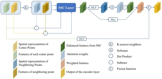
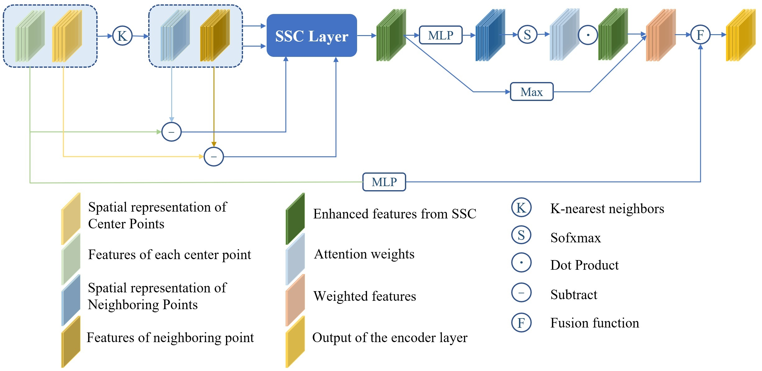
3.1. Spatial-Semantic Cross-Correction Module

Figure 2 shows the structure of our SSC module which can be decomposed into two parts: a semantic-aware spatial block to encode spatial geometric features and an attention block to extract high-level semantic information. Each block first aggregates nearest neighbors to acquire preliminary spatial geometric and semantics. The neighboring information clustered based on single criterion can introduce outliers or redundancies to some extent. Here, we associate the two branches together. The spatial geometric is rectified with position offsets inferred from semantics and vice versa. With such an in-depth feature learning style, the representation ability of the descriptor will be improved, and robust non-local features can finally be extracted to realize high-precision semantic segmentation.

3.1.1. Semantic-Aware Spatial Block

Given a point cloud with n points, their coordinates and acquired features can be denoted as P = { p 1 , , p i , , p n } R 3 and F = { f 1 , , f i , , f n } R N , respectively. As shown in Figure 2, we firstly perform k-nearest neighboring (kNN) to search K candidate neighborhoods denoted as { p i 1 , , p i k , , p i K } and { f i 1 , , f i k , , f i K } . Neighbors only based on Euclidean distance may bring in noisy points, so we affiliate with semantic information to revise the neighboring points. Then, the K neighbors and its center points construct a cluster to describe the local geometry. The elements of the cluster consist of four parts: point-wise distance-based neighbors p i k , neighbors rectified with semantic information h i k , the relative coordinates r i k and distances d i k . The cluster characteristics are fed into a shared MLP to generate feature map G = { g 1 , g 2 , , g K } to represent the geometric information.
The graphical representation of our semantic-aware spatial block is shown in Figure 2 (blue part). Three-dimensional (3D) x-y-z coordinates are natural elements for point clouds. This block encodes local spatial structures with a geometrical relationship from both distance and semantic approximable neighbors. We have demonstrated its effect in ablation study.

3.1.2. Attention Block

We have investigated two questions in Section 1, and this part is the solution to the second one. Our modified attention block is designed to better refine semantic information for local feature learning. The attention mechanism can help update point representation by assigning weights to different neighbors. To capture local representation, feature difference is taken as a constraint to select key information. However, only considering the feature difference as the criterion will introduce redundancy, and the spatial geometric relationship should play a role in correcting neighboring features.
Here, we combine this idea with point-wise based methods. Different from the previous feature difference, this paper appends the distance factor by calculating a distance-aware semantic deformation to refine the weight constraint:
Δ f i k = M f { ( p i p i k ) , p i p i k , ( p i h i k ) , p i h i k } ,
where Δ f i k represents the semantic deformation, and M f is a shared MLP.
Then, the deformable neighboring feature can be denoted as ν i k = f i k + Δ f i k , and the attention weight of each neighboring point is computed as follows:
α i k = M α { M g 1 ( f i , f i k ) , M g 2 ( f i , ν i k ) } ,
where M g i ( . , . ) are mapping functions to assess the effects of neighbors, and M α is the softmax function.
After the above operations, the feature of each neighboring point is recounted as follows:
f ˜ i k = α i k · ( M g { f i k , ν i k } ) ,
where M g performs an MLP operation with a ReLU activation. The output of the semantic context encoding is the new set of high-level neighboring features, which softly selects the positive information by a set of adaptive attention weights controlled by the modified feature difference.
The encoding procedures of spatial location and semantic context are not isolated in this Spatial–Semantic Cross-correction module. In this way, geometric and semantic information can be sufficiently exploited to acquire improved local feature representation.

3.2. Feature Aggregation

The SSC module explores correlation to represent scenes more effectively with augmented spatial geometric patterns and high-level semantic information. Given the feature maps of geometric representation G = { g 1 , , g k , , g K } and semantic context F ˜ i = { f ˜ i 1 , f ˜ i 2 , , f ˜ i k , , f ˜ i K } generated by the SSC module in Section 3.1, we use a feature fusion strategy to aggregate them:
Φ i = ψ ( f ˜ i k , r i k ) ,
where ψ represents concatenate operation.
Once the aggregated features Φ i = { φ i 1 , , φ i k , , φ i K } are obtained, we firstly perform a vector max operator to collect the most prominent neighbors,
Φ m a x = M A X ( Φ i ) .
Considering max-pooling operation tends to save features in a hard way, we insistently borrow an attention mechanism to obtain useful features abandoned by max-pooling. The attention weights can be calculated by a specific function i ( . , . ) where the learned attention scores play the role of a soft mask to automatically focus on the important features, and these neighboring features are summed in the following way:
Φ a t t = i = k K i ( φ i k , W ) · φ i k ,
where i ( , . , ) consists of a shared MLP followed by softmax, and W is the learnable weights of the shared MLP.
Then, the maximum and attentive features are combined,
Φ c o m = M L P s { Φ m a x , Φ a t t } ,
Finally inspired by the idea of ResNet [29], skip connection is added to implement the cross-promotion features:
Φ ˜ i = η ( F i ) + Φ c o m ,
where η is the function consisting of a shared MLP to improve F i and guarantee the same dimension with Φ c o m .

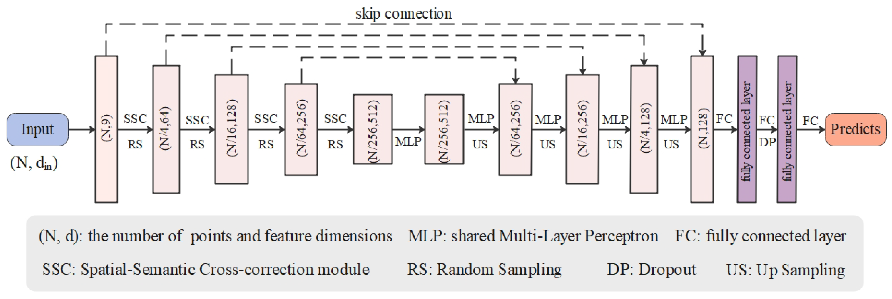
3.3. Our Network Architecture

This paper concentrates on improving the representation ability of the descriptor. We adopt the described module to construct the SSI-Net, shown in Figure 3, which follows the encoder–decoder structure to acquire multiple-scale features. The input of this network is a large-scale point cloud with a dimension of N × d i n where N is the number of points, and d i n is the feature dimension of each input point represented by its 3D coordinates and color information. The input is first fed into a fully connected layer to extract per-point features, and then, several encoding layers and decoding layers are used to learn rich feature representation. Finally, three fully connected layers and a dropout layer are appended to predict the semantic labels of the input.
The structure settings refer to the work [10] as follows:
Encoding layer: Each encoding layer adopts a given sampling ratio ((4, 4, 4, 4, 2) for S3DIS, and (4, 4, 4, 4) for SemanticKITTI) to gradually reduce the point size, and the output dimensions of each layer are ( 16 , 64 , 128 , 256 , 512 ) and ( 16 , 64 , 128 , 256 ) accordingly.
Decoding layer: The decoding layer used after the encoding layer is to restore the size of the input point cloud via a hierarchical propagation. Each decoding layer uses skip connection to help facilitate the feature extraction which concatenates the interpolated features with the features from the set abstraction layer to reduce information loss.
Semantic prediction: Semantic segmentation generates one label for each point of the input point cloud. After restoring to the original size, three fully connected layers followed by one dropout layer with a drop ratio of 0.5 are joined to predict the final semantic labels.

4. Experiments

In this section, we demonstrate how our method can be trained to perform semantic segmentation on point clouds and divide experimental descriptions into three parts. First, some necessary settings about our experiments are provided for comparison with the state-of-the-art. Second, detailed quantitative and qualitative results on different datasets are shown to illustrate the performance. Finally, ablation studies are performed to explain the selection of our network design.

4.1. Experimental Settings

Evaluation Metrics: The mean Intersection-over-Union (mIoU), the average value of Intersection over Union (IoU) for each semantic class, the overall accuracy (OA), and the average class accuracy (mAcc) are common standard scores to evaluate the semantic segmentation performance.
Datasets: This work targets an accurate semantic segmentation on large-scale point cloud scenes. To validate the proposed SSI-Net, we conduct experiments on some indoor and outdoor datasets.
1. Evaluation on S3DIS: The Stanford Large-Scale 3D Indoor Spaces (S3DIS) dataset is derived from real 3D scans and extensively used by lots of jobs. The S3DIS dataset includes 271 rooms from six areas containing 13 classes of objects typically encountered in an indoor scene: ceiling, floor, wall, beam, column, window, door, table, chair, sofa, bookcase, board, and clutter. Points in this dataset provide both 3D coordinates and color information. In the experiment, the number of input points on this dataset is set as 4096 10 . To evaluate the semantic segmentation results on S3DIS, we provide evaluation on Area 5 and 6-fold cross-validation results to compare the performances with certain state-of-the-art networks. The mACC, OA, and mIoU of the overall classes are compared in this paper.
2. Evaluation on SemanticKITTI: SemanticKITTI is a large-scale outdoor scene dataset which is based on the KITTI odometry dataset showing inner city traffic and residential areas but also highway scenes and countryside roads. There are 22 sequences ( 00 10 as the training set, and 11 21 as the test set) which are annotated in 19 semantic classes: road, sidewalk, parking, other-ground, building, car, truck, bicycle, motorcycle, other-vehicle, vegetation, trunk, terrain, person, bicyclist, motorcyclist, fence, pole, and traffic-sign. The raw point cloud contains 3D coordinates information. The number of input points is set as 4096 11 in the experiment. For this dataset, the mIoU and IoU of each class are taken as the evaluation metrics.
Training Settings: Our experiments have been performed with Python 3.6, Tensorflow 1.12 GPU version and trained for 100 epochs. During training, the batch size is set as 4, and the Adam optimizer is used. The initial learning rate is 0.01 and decays with a rate of 0.5 after every 10 epochs.

4.2. Performance Comparison

4.2.1. Results of S3DIS

This part shows the results on the S3DIS compared with different methods under the two evaluation modes mentioned in Section 4.1. Table 1 presents the results tested on Area 5. Our SSI-Net achieves the best performance in terms of mACC  ( 73.2 % ) and mIoU ( 65.1 % ) compared to these methods that supply evaluation on Area 5. The mIoU has improved by 3.7 % relative to the latest BoundaryAwareGEM [30], and the mACC has increased by 6.2 % over PointWeb [20]. The OA value of SSI-Net is 0.1 % lower than ELGS [31] which builds a more complex structure with graph attention block, the spatial-wise and channel-wise attention and is designed for small-scale point cloud processing. Moreover, most of the compared methods in the table prefer the farthest point sampling (FPS) as it leads to less information loss in comparison to random sampling. For better comparison, Table 2 shows the IoU value of each class of S3DIS on Area 5 from which one can see that our SSI-Net achieves the best performance on some complex structures such as a table, sofa, and bookcase.
Table 3 gives the results on the 6-fold cross-validation compared with PointNet [17], RSNet [36], 3P-RNN [37], PointCNN [32], ShellNet [38], PointWeb [20], KPConv r i g i d [39], KPConv d e f o r m [39], PointASNL [22], and RandLA [10]. Approaches [10,17,20,22,38] are classified into point-based methods. Other researchers such as [32,39] utilize convolution-like operation to improve feature representation. The mACC of SSI-Net rises to 82.3 % and surpasses the listed results in this test mode. However, the scores of OA and mIoU are slightly inferior to PointASNL [22] and KPConv d e f o r m [39], respectively. Most of the methods return similarly high IoU values for simple classes. Significant differences distribute in classes with complex structures such as table, chair and sofa.
Detailed semantic segmentation results for each area on the S3DIS dataset with 6-fold cross-validation are shown in Table 4 to better represent the performance of our approach.

4.2.2. Results of SemanticKITTI

SemanticKITTI is a challenging dataset. Table 5 reports the quantitative results of SSI-Net on this dataset compared with some representative methods. The mIoU of our method achieves the best value of 55.4 % , which surpasses most point-based methods [9,10,18,22,40,41] by a large margin. From Table 4, one can see that the projection-based methods [42,43,44,45] are superior to the point-based methods on the whole. However, our SSI-Net also outperforms these mentioned projection-based methods. For example, the mIoU value increases by 1.1 % compared to the best projection-based method [45]. It obtains the maximum mIoU in 11 out of the 19 categories: particularly the values of the truck and motorcycle, which are much higher than the second ones. We attribute this to the active cross-correction of the spatial and semantic information developed by our SSC module.
Figure 4, Figure 5 and Figure 6 present concerned illustrations of the SemanticKITTI dataset. Figure 4 shows some qualitative results on the validation set. SemanticKITTI provides an unprecedented number of scans covering the full 360 degree field-of-view of the employed automotive LiDAR, and we choose four scans from sequence 08 to reveal a contrast of segmentation results. Pictures in the first row are the ground truths, and these in the second row are the outputs of SSI-Net. Figure 5 shows the inference time on sequence 08 of SemanticKITTI and the overall mIoU to demonstrate the efficiency of the proposed method.
Sequences 11∼21 are used as a test set showing a large variety of challenging traffic situations and environment types. Figure 6 exhibits some qualitative results of online test (sequences 11∼21) in 2D panorama views.

4.3. Ablation Studies

Effect of each unit: To demonstrate the effect of each component: semantic-aware spatial location encoding, attentional semantic encoding, and feature aggregation block, we perform the following ablation studies on Area 5 of the S3DIS dataset and SemanticKITTI datset:
(1)
Removing the semantic-aware information of spatial location encoding: this part aims to encode more detailed local geometry with position and high-level information;
(2)
Replacing the attentional semantic encoding by general MLP layers;
(3)
Aggregating local features only by max operation.
Results of this part are shown in Table 6: (1) The encoder with our full units reaches the best mIoU; (2) The greatest impact on mIoU is caused by the removing of an attentional semantic block probably because attention mechanism and neighboring deformation can help aggregate key semantic information discarded by random sampling.
Selection of spatial encoding block: As described in Section 3.1.1, the semantic-aware spatial block can be expressed as follows:
g i k = M s { p i k , h i k , ( p i p i k ) , p i p i k , ( p i h i k ) , p i h i k } .
We perform other experiments for the selection of this module:
(1)
Encoding the neighboring points p i k and deformable neighboring points h i k ;
(2)
Encoding the relative position: p i p i k and p i h i k , and corresponding Euclidean distance: p i p i k and p i h i k ;
(3)
Encoding the point p i , the relative position: p i p i k and p i h i k , and Euclidean distance: p i p i k and p i h i k ;
(4)
Encoding the neighboring points: p i k and h i k , the relative position: p i p i k and p i h i k , and the Euclidean distance: p i p i k and p i h i k .
Table 7 compares the mIoU values with different selections: (1) encoding the neighboring points, the relative position and the Euclidean distance outputs the highest mIoU; (2) the neighboring points play an important role in our spatial location encoding block.
FPS vs. RS: We compare the mIoU and IoU value of each class in this part, Table 8. The mIoU value of RS is only lower than FPS by 0.1 % ; however, as we know, the FPS is much less efficient than RS. Thus, we choose random sampling in our design.

5. Conclusions

This paper pays attention to large-scale semantic segmentation on point clouds to provide reliable information for indoor and outdoor semantic understanding such as autonomous vehicles that need detailed objects mapping in urban roads. Specifically, our proposed architecture SSI-Net is built on an SSC module that focuses on a more effective feature description via a spatial and semantic cross-correction manner. By mutually revising the neighboring information, robust representation can be obtained to support our work. Experimental results on S3DIS and SemanticKITTI datasets achieve the state-of-the-art performance compared to relevant methods. However, this work also has its limitations. We only consider simple characteristics of point clouds (i.e., distance and relative position), which may face ambiguities of feature representation in more complex scenes. For instance, this kind of geometric representation cannot well handle the situation where different objects are cluttered closely in a table. In future work, we will focus on these problems by improving boundary information or acquiring more semantic expression with cross-modality segmentation et al., and we will further promote its combination with more 3D tasks such as 3D reconstruction, real-time localization and point cloud pose estimation.

Author Contributions

Y.Z. made substantial contributions to the conception, design of the work, and the analysis of the performance; J.Z. played an important role in revising the manuscript critically; J.M. and S.X. directed the main work. All authors have read and agreed to the published version of the manuscript.

Funding

This research was funded by the Hebei Natural Science Foundation (Grant number [F2020202045]), in part by the National Natural Science Foundation of China (Nos. U21A20515, 62271074, 61972459, 61971418, U2003109, 62171321, 62071157, 62162044 and 32271983) and in part by the Open Research Fund of Key Laboratory of Space Utilization, Chinese Academy of Sciences (No. LSU-KFJJ-2021-05), and this work was supported by the Open Projects Program of National Laboratory of Pattern Recognition.

Institutional Review Board Statement

Not applicable.

Informed Consent Statement

Not applicable.

Data Availability Statement

The data presented in this study are available on request from the corresponding author.

Conflicts of Interest

The authors declare no conflict of interest. This work has not been published elsewhere in any form or language. The results presented in this article are clear and honest.

References

  1. Sun, W.; Zhang, Z.; Huang, J. RobNet: Real-time road-object 3D point cloud segmentation based on SqueezeNet and cyclic CRF. Soft Comput. 2020, 24, 5805–5818. [Google Scholar] [CrossRef]
  2. Hao, F.; Li, J.; Song, R.; Li, Y.; Cao, K. Mixed Feature Prediction on Boundary Learning for Point Cloud Semantic Segmentation. Remote Sens. 2022, 14, 4757. [Google Scholar] [CrossRef]
  3. Lan, S.; Yu, R.; Yu, G.; Davis, L.S. Modeling local geometric structure of 3d point clouds using geo-cnn. In Proceedings of the IEEE Conference on Computer Vision and Pattern Recognition, Long Beach, CA, USA, 15–20 June 2019. [Google Scholar]
  4. Wu, W.; Qi, Z.; Fuxin, L. Pointconv: Deep convolutional networks on 3d point clouds. In Proceedings of the IEEE Conference on Computer Vision and Pattern Recognition, Long Beach, CA, USA, 15–20 June 2019. [Google Scholar]
  5. He, T.; Shen, C.; Hengel, A. Dynamic Convolution for 3D Point Cloud Instance Segmentation. arXiv 2021, arXiv:2107.08392. [Google Scholar] [CrossRef] [PubMed]
  6. Wang, Y.; Sun, Y.; Liu, Z.; Sarma, S.E.; Bronstein, M.M.; Solomon, J.M. Dynamic graph cnn for learning on point clouds. ACM Trans. Graph. (TOG) 2019, 38, 1–12. [Google Scholar] [CrossRef] [Green Version]
  7. Li, G.; Muller, M.; Thabet, A.; Ghanem, B. DeepGCNs: Can gcns go as deep as cnns? In Proceedings of the IEEE/CVF International Conference on Computer Vision, Seoul, Korea, 27 October–2 November 2019. [Google Scholar]
  8. Wang, L.; Huang, Y.; Hou, Y.; Zhang, S.; Shan, J. Graph attention convolution for point cloud semantic segmentation. In Proceedings of the IEEE Conference on Computer Vision and Pattern Recognition, Long Beach, CA, USA, 15–20 June 2019. [Google Scholar]
  9. Landrieu, L.; Simonovsky, M. Large-scale point cloud semantic segmentation with superpoint graphs. In Proceedings of the IEEE Conference on Computer Vision and Pattern Recognition, Salt Lake City, UT, USA, 18–23 June 2018. [Google Scholar]
  10. Hu, Q.; Yang, B.; Xie, L.; Rosa, S.; Guo, Y.; Wang, Z.; Trigoni, N.; Markham, A. Learning Semantic Segmentation of Large-Scale Point Clouds with Random Sampling. IEEE Trans. Pattern Anal. Mach. Intell. 2021, 44, 8338–8354. [Google Scholar] [CrossRef] [PubMed]
  11. Boulch, A.; Guerry, J.; Le Saux, B.; Audebert, N. Snapnet: 3d point cloud semantic labeling with 2d deep segmentation networks. Comput. Graph. 2018, 71, 189–198. [Google Scholar] [CrossRef]
  12. Tchapmi, L.; Choy, C.; Armeni, I.; Gwak, J.; Savarese, S. Segcloud: Semantic segmentation of 3d point clouds. In Proceedings of the 2017 International Conference on 3D Vision, Qingdao, China, 10 October 2017; pp. 537–547. [Google Scholar]
  13. Wang, P.S.; Liu, Y.; Guo, Y.X.; Sun, C.Y.; Tong, X. O-cnn: Octree-based convolutional neural networks for 3d shape analysis. ACM Trans. Graph. (TOG) 2017, 36, 1–11. [Google Scholar] [CrossRef] [Green Version]
  14. Meng, H.Y.; Gao, L.; Lai, Y.K.; Manocha, D. Vv-net: Voxel vae net with group convolutions for point cloud segmentation. In Proceedings of the IEEE/CVF International Conference on Computer Vision, Seoul, Korea, 27 October–2 November 2019. [Google Scholar]
  15. Riegler, G.; Osman Ulusoy, A.; Geiger, A. Octnet: Learning deep 3d representations at high resolutions. In Proceedings of the IEEE Conference on Computer Vision and Pattern Recognition, Honolulu, HI, USA, 21–26 July 2017; 2017. [Google Scholar]
  16. Park, J.; Kim, C.; Jo, K. PCSCNet: Fast 3D Semantic Segmentation of LiDAR Point Cloud for Autonomous Car using Point Convolution and Sparse Convolution Network. arXiv 2022, arXiv:2202.10047. [Google Scholar] [CrossRef]
  17. Qi, C.R.; Su, H.; Mo, K.; Guibas, L.J. Pointnet: Deep Learning on Point Sets for 3D Classification and Segmentation. In Proceedings of the IEEE Conference on Computer Vision and Pattern Recognition, Honolulu, HI, USA, 21–26 July 2017; pp. 652–660. [Google Scholar]
  18. Qi, C.R.; Yi, L.; Su, H.; Guibas, L.J. PointNet++: Deep hierarchical feature learning on point sets in a metric space. In Proceedings of the 2017 Conference on Neural Information Processing Systems, Long Beach, CA, USA, 4–9 December 2017. [Google Scholar]
  19. Zhang, D.; He, F.; Tu, Z.; Zou, L.; Hen, Y. Pointwise geometric and semantic learning network on 3D point clouds. Integr.-Comput.-Aided Eng. 2020, 27, 57–75. [Google Scholar] [CrossRef]
  20. Zhao, H.; Jiang, L.; Fu, C.W.; Jia, J. Pointweb: Enhancing local neighborhood features for point cloud processing. In Proceedings of the IEEE Conference on Computer Vision and Pattern Recognition, Long Beach, CA, USA, 15–20 June 2019. [Google Scholar]
  21. Han, W.; Wen, C.; Wang, C.; Li, X.; Li, Q. Point2Node: Correlation learning of dynamic-node for point cloud feature modeling. Proc. AAAI Conf. Artif. Intell. 2020, 34, 10925–10932. [Google Scholar] [CrossRef]
  22. Yan, X.; Zheng, C.; Li, Z.; Wang, S.; Cui, S. PointASNL: Robust point clouds processing using nonlocal neural networks with adaptive sampling. In Proceedings of the 2020 IEEE/CVF Conference on Computer Vision and Pattern Recognition, Seoul, Korea, 14–19 June 2020. [Google Scholar]
  23. Chen, J.; Kakillioglu, B.; Velipasalar, S. Background-Aware 3D Point Cloud Segmentation with Dynamic Point Feature Aggregation. arXiv 2021, arXiv:2111.07248. [Google Scholar]
  24. Chen, C.; Chen, Z.; Zhang, J.; Tao, D. SASA: Semantics-Augmented Set Abstraction for Point-based 3D Object Detection. arXiv 2022, arXiv:2201.01976. [Google Scholar] [CrossRef]
  25. Srivastava, S.; Sharma, G. Exploiting local geometry for feature and graph construction for better 3d point cloud processing with graph neural networks. In Proceedings of the IEEE International Conference on Robotics and Automation (ICRA), Xi’an, China, 5 June 2021. [Google Scholar]
  26. Rethage, D.; Wald, J.; Sturm, J.; Navab, N.; Tombari, F. Fully-convolutional point networks for large-scale point clouds. In Proceedings of the 15th European Conference on Computer Vision, Munich, Germany, 8–14 September 2018. [Google Scholar]
  27. Chen, S.; Niu, S.; Lan, T.; Liu, B. PCT: Large-scale 3D point cloud representations via graph inception networks with applications to autonomous driving. In Proceedings of the 26th IEEE International Conference on Image Processing (ICIP), Taipei, Taiwan, 22–25 September 2019. [Google Scholar]
  28. Luo, C.; Li, X.; Cheng, N.; Li, H.; Lei, S.; Li, P. MVP-Net: Multiple View Pointwise Semantic Segmentation of Large-Scale Point Clouds. arXiv 2022, arXiv:2201.12769. [Google Scholar]
  29. He, K.; Zhang, X.; Ren, S.; Sun, J. Deep residual learning for image recognition. In Proceedings of the IEEE Conference on Computer Vision and Pattern Recognition, Las Vegas, NV, USA, 27–30 June 2018. [Google Scholar]
  30. Gong, J.; Xu, J.; Tan, X.; Zhou, J.; Qu, Y.; Xie, Y.; Ma, L. Boundary-aware geometric encoding for semantic segmentation of point clouds. arXiv 2021, arXiv:2101.02381. [Google Scholar] [CrossRef]
  31. Wang, X.; He, J.; Ma, L. Exploiting local and global structure for point cloud semantic segmentation with contextual point representations. Adv. Neural Inf. Process. Syst. 2019, 32, 4571–4581. [Google Scholar]
  32. Li, Y.; Bu, R.; Sun, M.; Wu, W.; Di, X.; Chen, B. Pointcnn: Convolution on X-transformed points. In Proceedings of the 2018 Conference on Neural Information Processing Systems, Montreal, QC, Canada, 3–8 December 2018. [Google Scholar]
  33. Wang, S.; Suo, S.; Ma, W.; Pokrovsky, A.; Urtasun, R. Deep parametric continuous convolutional neural networks. In Proceedings of the IEEE Conference on Computer Vision and Pattern Recognition, Salt Lake City, UT, USA, 18–23 June 2018. [Google Scholar]
  34. Choy, C.; Gwak, J.; Savarese, S. 4d spatio-temporal convnets: Minkowski convolutional neural networks. In Proceedings of the IEEE Conference on Computer Vision and Pattern Recognition, Long Beach, CA, USA, 15–20 June 2019. [Google Scholar]
  35. Liu, Y.; Hu, Q.; Lei, Y.; Xu, K.; Li, J.; Guo, Y. Box2Seg: Learning Semantics of 3D Point Clouds with Box-Level Supervision. arXiv 2022, arXiv:2201.02963. [Google Scholar]
  36. Huang, Q.; Wang, W.; Neumann, U. Recurrent slice networks for 3d segmentation of point clouds. In Proceedings of the IEEE Conference on Computer Vision and Pattern Recognition, Salt Lake City, UT, USA, 18–23 June2018. [Google Scholar]
  37. Ye, X.; Li, J.; Huang, H.; Du, L.; Zhang, X. 3D recurrent neural networks with context fusion for point cloud semantic segmentation. In Proceedings of the 15th European Conference on Computer Vision, Munich, Germany, 8–14 September 2018. [Google Scholar]
  38. Zhang, Z.; Hua, B.S.; Yeung, S.K. Shellnet: Efficient point cloud convolutional neural networks using concentric shells statistics. In Proceedings of the IEEE Conference on Computer Vision and Pattern Recognition, Long Beach, CA, USA, 15–20 June 2019. [Google Scholar]
  39. Thomas, H.; Qi, C.R.; Deschaud, J.; Marcotegui, B.; Goulette, F.; Guibas, L.J. Kpconv: Flexible and deformable convolution for point clouds. In Proceedings of the IEEE/CVF International Conference on Computer Vision, Seoul, Korea, 27 October–2 November 2019. [Google Scholar]
  40. Su, H.; Jampani, V.; Sun, D.; Maji, S.; Kalogerakis, E.; Yang, M.; Kautz, J. SPLATNet: Sparse lattice networks for point cloud processing. In Proceedings of the IEEE Conference on Computer Vision and Pattern Recognition, Salt Lake City, UT, USA, 18–23 June 2018. [Google Scholar]
  41. Tatarchenko, M.; Park, J.; Koltun, V.; Zhou, Q. Tangent convolutions for dense prediction in 3D. In Proceedings of the IEEE Conference on Computer Vision and Pattern Recognition, Salt Lake City, UT, USA, 18–23 June 2018. [Google Scholar]
  42. Wu, B.; Wan, A.; Yue, X.; Keutzer, K. Squeezeseg: Convolutional neural nets with recurrent crf for real-time road-object segmentation from 3D lidar point cloud. In Proceedings of the 2018 IEEE International Conference on Robotics and Automation (ICRA), Brisbane, Australia, 21–25 May 2018. [Google Scholar]
  43. Wu, B.; Zhou, X.; Zhao, S.; Yue, X.; Keutzer, K. Squeezesegv2: Improved model structure and unsupervised domain adaptation for road-object segmentation from a lidar point cloud. In Proceedings of the International Conference on Robotics and Automation (ICRA), Montreal, QC, Canada, 20–24 May 2019. [Google Scholar]
  44. Behley, J.; Garbade, M.; Milioto, A.; Quenzel, J.; Behnke, S.; Stachniss, C.; Gall, J. SemanticKITTI: A dataset for semantic scene understanding of lidar sequences. In Proceedings of the IEEE/CVF International Conference on Computer Vision, Seoul, Korea, 27 October–2 November 2019. [Google Scholar]
  45. Zhang, Y.; Zhou, Z.; David, P.; Yue, X.; Xi, Z.; Gong, B.; Foroosh, H. Polarnet: An 10 improved grid representation for online lidar point clouds semantic segmentation. In Proceedings of the IEEE/CVF Conference on Computer Vision and Pattern Recognition, Seattle, WA, USA, 13–19 June 2020. [Google Scholar]
  46. Milioto, A.; Vizzo, I.; Behley, J.; Stachniss, C. RangeNet++: Fast and accurate lidar semantic segmentation. In Proceedings of the 2019 IEEE/RSJ International Conference on Intelligent Robots and Systems (IROS), Macao, China, 3–8 November 2019. [Google Scholar]
  47. Cortinhal, T.; Tzelepis, G.; Aksoy, E.E. SalsaNext: Fast semantic segmentation of lidar point clouds for autonomous driving. arXiv 2020, arXiv:2003.03653. [Google Scholar]
  48. Rosu, R.A.; Sch¨utt, P.; Quenzel, J.; Behnke, S. LatticeNet: Fast point cloud segmentation using permutohedral lattices. arXiv 2019, arXiv:1912.05905. [Google Scholar]
Figure 1. Semantic predictions of LiDAR scans. From left to right are the results of SPG [9], RandLA [10], SSI-Net, and ground truth.
Remotesensing 14 06022 g001
Figure 2. Structure of the proposed Spatial–Semantic Cross-correction module.
Remotesensing 14 06022 g002
Figure 3. Structure of the proposed Spatial–Semantic Cross-correction module.
Remotesensing 14 06022 g003
Figure 4. Qualitative results of our SSI-Net on the validation set of SemanticKITTI. Red rectangles represent the failure cases.
Remotesensing 14 06022 g004
Figure 5. Inference time comparison on sequence 08 of SemanticKITTI and mIoU of SemanticKITTI of PointNet [17], PointNet++ [18], SPG [9], RandLA [10] and SSI-Net (ours).
Remotesensing 14 06022 g005
Figure 6. Qualitative results of online test on sequence 11 21 .
Remotesensing 14 06022 g006
Table 1. Results (%) on S3DIS evaluated on Area 5.
MethodsOAmACCmIoU
PointNet [17]-49.041.1
SegCloud [12]-57.448.9
PointCNN [32]85.963.957.3
SPG [9]86.466.558.0
PCCN [33]-67.058.3
PointWeb [20]86.966.660.3
ELGS [31]88.4-60.1
MinkowskiNet20 [34]-62.669.6
MinkowskiNet32 [34]-65.471.7
BoundaryAwareGEM [30]--61.4
DPFA [23]87.4-53.0
DPFA+BF Reg [23]88.0-55.2
3D GrabCut [35]--57.7
Box2Seg (AST) [35]--60.4
SSI-Net88.373.265.1
Table 2. IoU (%) of each class of S3DIS evaluated on Area 5.
MethodsCeil.FloorWallBeamCol.Wind.DoorTableChairSofaBook.BoardClut.
PointNet [17]88.897.369.80.053.946.310.852.658.940.35.926.433.2
SegCloud [12]90.196.169.90.018.438.423.175.970.458.440.913.041.6
PointCNN [32]92.398.279.40.017.622.862.174.480.631.766.762.156.7
SPG [9]89.496.978.10.042.848.961.684.775.469.852.62.152.2
PCCN [32]92.396.275.90.35.9869.563.566.965.647.368.959.146.2
PointWeb [20]92.098.579.40.021.159.934.876.388.346.969.364.952.5
3D GrabCut [35]80.388.769.60.028.861.035.266.571.769.269.761.748.2
Box2Seg (AST) [35]82.092.070.80.028.861.938.171.485.374.368.463.648.0
DPFA [23]93.798.775.50.014.550.131.873.773.413.755.557.151.2
DPFA+BF Reg [23]93.098.680.20.014.755.842.872.373.527.355.953.050.5
SSI-Net93.197.781.70.024.561.954.279.487.767.070.472.056.0
Table 3. Results (%) on S3DIS dataset with 6-fold cross-validation.
MethodsOAmACCmIoUCeil.FloorWallBeamCol.Wind.DoorTableChairSofaBook.BoardClut.
PointNet [17]78.666.247.688.088.769.342.423.147.551.654.142.09.638.229.435.2
RSNet [36]-66.556.592.592.878.632.834.451.668.159.760.116.450.244.952.0
3P-RNN [37]86.9-56.392.993.873.142.525.947.659.260.466.724.857.036.751.6
PointCNN [32]88.175.665.494.897.375.863.351.758.457.271.669.139.161.252.258.6
ShellNet [38]87.1-66.890.293.679.960.444.164.952.971.684.753.864.648.659.4
PointWeb [20]87.376.266.793.594.280.852.441.364.968.171.467.150.362.762.258.5
KPConv r i g i d [39]-78.169.693.792.082.562.549.565.777.357.864.068.871.760.159.6
KPConv d e f o r m [39]-79.170.693.692.483.163.954.366.176.657.864.069.374.961.360.3
PointASNL [22]88.879.068.795.397.981.947.048.067.370.571.377.850.760.463.062.8
RandLA [10]88.082.070.093.196.180.662.448.064.469.469.476.460.064.265.960.1
SSI-Net88.082.370.593.796.880.161.944.065.069.772.874.667.663.266.060.6
Table 4. Detailed results (%) for each area on S3DIS dataset with 6-fold cross-validation.
Testing AreaOAmACCmIoUCeil.FloorWallBeamCol.Wind.DoorTableChairSofaBook.BoardClut.
Area189.275.787.696.395.177.154.351.980.183.473.381.476.562.870.467.7
Area284.255.470.889.095.576.821.426.652.264.649.860.356.050.028.349.8
Area391.179.289.495.798.281.470.233.382.188.574.784.885.074.588.673.0
Area485.162.176.694.197.077.839.948.831.860.568.677.765.546.139.760.0
Area588.365.173.293.197.781.70.024.561.954.279.487.767.070.472.056.0
Area691.980.092.296.797.584.482.072.080.986.475.984.262.172.475.170.8
Table 5. Semantic segmentation results (%) on the SemanticKITTI dataset.
MethodsmIoURoadSidewalkParkingOther-groundBuildingCarTruckBicycleMotorcycleOther-VehicleVegetationTrunkTerrainPersonBicyclistMotorcyclistFencePoleTraffic-sign
PointNet [17]14.661.635.715.81.441.446.30.11.30.30.831.04.617.60.20.20.012.92.43.7
SPG [9]17.445.028.50.60.664.349.30.10.20.20.848.927.224.60.32.70.120.815.90.8
SPLATNet [40]18.464.639.10.40.058.358.20.00.00.00.071.19.919.30.00.00.023.15.60.0
PointNet++ [18]20.172.041.818.75.662.353.70.91.90.20.246.513.830.00.91.00.016.96.08.9
TangentConv [41]40.983.963.933.415.483.490.815.22.716.512.179.549.358.123.028.48.149.035.828.5
SqueezeSeg [42]29.585.454.326.94.557.468.83.316.04.13.660.024.353.712.913.10.929.917.524.5
SqueezeSegV2 [43]39.788.667.645.817.773.781.813.418.517.914.071.835.860.220.125.13.941.120.236.3
DarkNet21Seg [44]47.491.474.057.026.481.985.418.626.226.515.677.648.463.631.833.64.052.336.050.0
DarkNet53Seg [44]49.991.874.664.827.984.186.425.524.532.722.678.350.164.036.233.64.755.038.952.2
RangeNet53++ [46]52.291.875.265.027.887.491.425.725.734.423.080.555.164.638.338.84.858.647.955.9
SalsaNext [47]54.590.974.058.127.887.990.921.736.429.519.981.861.766.352.052.716.058.251.758.0
LatticeNet [48]52.288.873.864.625.686.988.643.412.020.824.876.457.954.734.239.960.955.241.542.7
PointASNL [22]46.887.474.324.31.883.187.939.00.025.129.284.152.270.634.257.60.043.957.836.9
RandLA-Net [10]53.990.773.760.320.486.994.240.126.025.838.981.461.366.849.248.27.256.349.247.7
PolarNet [45]54.390.874.461.721.790.093.822.940.330.128.584.065.567.843.240.25.667.851.857.5
MVP-Net [28]53.991.475.961.425.685.892.720.237.217.713.883.264.569.350.055.812.955.251.859.2
SSI-Net55.492.212.936.972.027.855.066.40.092.942.279.60.889.554.286.866.076.158.641.9
Table 6. Ablation studies on Area 5 of S3DIS and SemanticKITTI (%).
S3DISSemanticKITTI
MethodsOAmACCmIoUmIoU
Removing semantic-aware information86.172.263.653.8
Removing attentional semantic block85.271.861.951.7
Max operation86.773.063.152.9
With full units88.373.265.155.4
Table 7. Selection for spatial location encoding test on Area 5 of S3DIS and SemanticKITTI (%).
S3DISSemanticKITTI
MethodsmIoUmIoU
(1) { p i k , h i k } 63.552.0
(2) { ( p i p i k ) , p i p i k , ( p i h i k ) , p i h i k } 65.053.1
(3) { p i , ( p i p i k ) , p i p i k , ( p i h i k ) , p i h i k } 63.454.0
(4) { p i k , h i k , ( p i p i k ) , p i p i k , ( p i h i k ) , p i h i k } 65.155.4
Table 8. Effect of different sampling strategies (%).
SamplingsmIoUCeil.FloorWallBeamCol.Wind.DoorTableChairSofaBook.BoardClut.
Farthest Point Sampling (FPS)65.293.997.582.00.030.262.248.980.487.462.572.472.557.4
Random Sampling (RS)65.193.197.781.70.024.561.954.279.487.767.070.472.056.0
Publisher’s Note: MDPI stays neutral with regard to jurisdictional claims in published maps and institutional affiliations.

