Article

The Grain for Green Program Enhanced Synergies between Ecosystem Regulating Services in Loess Plateau, China

1
Key Laboratory of Land Surface Pattern and Simulation, Institute of Geographic Science and Natural Resources Research, Chinese Academy of Sciences, Beijing 100101, China
2
Faculty of Science and Engineering, The University of Nottingham Ningbo China, Ningbo 315100, China
*
Author to whom correspondence should be addressed.
Remote Sens. 2022, 14(23), 5940; https://doi.org/10.3390/rs14235940
Submission received: 17 October 2022 / Revised: 18 November 2022 / Accepted: 21 November 2022 / Published: 24 November 2022

Abstract

:
Decades of reckless deforestation have caused serious soil erosion and land desertification issues in the Loess Plateau (LP). “Grain for Green” Program (GFGP), one of the world’s largest ecological restoration projects, is crucial to improve the ecological environment. Previous studies have demonstrated that GFGP lowers soil erosion in the LP. However, there are trade-offs and synergies between ecological services. Does strengthening soil conservation prevent enhancing other ecosystem services? Consequently, can the GFGP improve many ecological services simultaneously? This study compares changes in NDVI prior to and following the implementation of the GFGP in LP to the enhancement of ecosystem services. During the research period, the LP’s overall vegetation cover rose significantly, particularly in the GFGP’s major counties. Significant improvements were made to ecosystem services such as carbon sequestration, soil conservation, and habitat quality. The GFGP enhanced the synergistic linkages between ecological services. The implementation of the GFGP decreased water yield, suggesting trade-offs with other ecosystem services. Additionally, we investigate regional trade-offs/synergies between ecosystem services and their influencing factors, which were influenced by topographic and climatic variables. To maximize the benefits of ecological restoration efforts, we need a deeper understanding of the relationships between ecosystem services and the mechanisms that drive them. Thus, policymakers can scientifically exert control over local influences on ecosystem services, either by boosting the provision of specific services or by limiting specific influences in order to maintain ecosystem stability.

1. Introduction

Ecosystem services (ESs) are commonly defined as natural ecosystems and the species that make up the system providing well-being to humans in order to meet the needs of human life [1]. ESs include not only the food and fresh water provided for human life, but more importantly, they support and maintain the diversity of biological species and purify the environment [2]. These provide the essential foundation for human survival and development. Human actions have harmed and degraded the ecosystem [3,4]. According to the United Nations Millennium Ecosystem Assessment report, 15 of the 24 ecological services [5], i.e., 60% of global ESs, are in danger of being degraded, owing to high population pressure and overexploitation of natural resources as a result of increasing urbanization [5]. Thus, such a decline in the capacity of ecosystems to provide services poses a significant threat to human well-being [6].
Ecosystem degradation could be observed at global and regional scales [7,8]. With rapid urbanization, the proportion of the global population living in urban areas is expected to reach 70% by 2050. Thus, urban areas are expanding while forest areas are shrinking, which has a negative impact on ecosystems [9,10,11]. Moreover, the rapid economic boom has progressively degraded ecosystem in China [12]. China has a diverse natural environment and ecosystem types [13]. So, there are challenges in solving ecosystem degradation in China. In recent decades, rapid urbanization and dramatic impacts of human activities have exacerbated ecological and environmental issues, including water shortage, soil erosion, land degradation, and reduced biodiversity [14]. For example, about 5.392 million km2 of land were deteriorated as a result of unreasonable human activity and adverse natural events, or nearly 56% of China’s land area [15,16]. Large-scale deforestation and land clearance have exacerbated soil erosion, severe land degradation, frequent droughts and floods, and a rapid deterioration of the biological ecosystem [17]. China’s soil erosion impacts 3.56 km2, or 37.1% of the country’s land area, according to the government’s second national remote sensing assessment on soil erosion, and the country loses nearly 5 billion tons of soil each year [18]. The natural ecology of the western region is deteriorating, primarily due to a shortage of available water. Desertification is increasing year by year and expanding to the east [17]. This has a detrimental effect on the western region’s economic growth and development, as well as on neighboring villages. Enhancing the ecological environment is a crucial issue that must be explored and resolved prior to the expansion and development of the western region. Thus, the scientific research focus has turned to the long-term viability of ESs.
Sustainable ecosystem services can be maintained by integrating ecological restoration projects into natural resource management at the local, regional, and global levels [19,20]. Ecological restoration efforts contribute to the enhancement of ESs by reversing environmental degradation due to human activity [21]. Thus, assessing ecological restoration projects’ contribution to ESs is critical for ensuring a sustainable supply of ecosystem services. To ensure the country’s ecological security and to attain carbon neutrality, the Chinese government has been implementing the world’s largest ecological restoration project, the “Grain for Green” Program (GFGP) [22]. The GFGP has designated the Loess Plateau (LP) as a priority pilot area [23]. The region has long been plagued by significant soil erosion and is regarded one of the world’s most degraded locations [24]. The LP’s ecosystem deterioration has resulted in a reduction in ESs as well as the ability to support human activities and long-term regional development. Increased forest land can improve ecosystem services such as sustained biodiversity, soil conservation, water balance, and socio-economic benefits [25]. In order to promote GFGP systematically and strengthen ecological construction and environmental protection, the government of the first round of GFGP selected key counties in each province with serious soil erosion and wind and sand disasters. By significantly increasing plant cover, minimizing water surface runoff and soil erosion, and sustaining soil fertility, the GFGP has made a considerable contribution to the improvement of the ecological environment and different ESs [26,27,28]. From the beginning of the project to the end of 2006, nearly 9 million ha of cropland were converted to forest/grassland [29]. However, there are trade-offs/synergies between the various ESs that are relevant. Moreover, there are potential conflicts between regional ecosystem services and human needs. There is a possibility that some ESs are increased at the expense of others, which can also lead to the decline of many other ESs [30]. For example, large-scale cropland has been afforested, and too much food has been traded for green [31]. While vegetation cover rises substantially, the food provisioning functions may be jeopardized. This further stimulates a potential conflict between human food demand and ecosystem function. Additionally, while mass planting of non-native monoculture tree species expands the size of the forest and grassland, it also uses more water. It may have a detrimental effect on how well ESs produce water [32]. This shows that it is uncertain if GFGP will enhance ESs and enhance human wellbeing. Large-scale ecological restoration initiatives have unanticipated ecological effects despite being beneficial to ecosystem services and the ecological environment. It is therefore vital to measure the contribution of GFGP to ESs both before and after its implementation. It is also difficult to identify the trade-offs and synergies between various ESs for the long-term stability of ecosystems and the benefit of human existence. This will assure the long-term viability of ESs and the efficacy of ecological restoration projects.
Most previous studies have confirmed that GFGP facilitates the improvement of ESs. Different studies have assessed ESs changes in the LP after GFGP, mainly using GIS and remote sensing approaches. For instance, most previous research that used long-term NDVI data came to the conclusion that the plant cover of the LP grew by 25% in the ten years after the implementation of the GFGP [33]. In addition to the vegetation cover, previous studies also focused on soil loss. Satellite imagery and the Universal Soil Loss Equation (USLE) were used to assess changes in soil conservation services in the LP between 2000 and 2008. The findings indicated that this ecosystem service has enhanced significantly as a result of revegetation [34]. The findings highlight the benefits of ecological restoration efforts as well as the need for adaptive management. Therefore, the improvement cannot be judged solely by the GFGP solely under the increase in vegetation cover or the overall improved trend of ESs. Based on the NDVI annual trend, several necessary ESs representing the LP were selected. In order to quantify the contribution made by GFGP to the restoration of the ecological environment, this study mainly selected the ecological regulation services in carbon sequestration, soil conservation, and water yield at the sub-watershed scale. With the sharp decline in biodiversity due to ecosystem degradation, this paper also supplements the consideration of ecosystem-supporting services: habitat quality [35]. Additionally, ecosystem services are not independent. Instead, they interact with each other, and there are trade-offs or synergistic relationships [36]. The blind pursuit of maximizing the benefits of a particular ecosystem service can compromise the benefits of other ecosystem supplies [37]. So, to better understand the contribution of GFGP to improving ecosystem services, it is vital to understand the trade-offs /synergies between ESs. However, the impact of GFGP on multiple ecosystem service alterations varies, and there is a lack of research on trade-offs/synergies between ESs. Additionally, the trade-offs and synergies between ESs vary by geography. Natural, anthropogenic, climatic, and socioeconomic variables will impact the ecosystem’s inherent changes, which are complicated. This study needs to assess the spatial heterogeneity of this underlying relationship in order to properly appreciate the tradeoffs/synergies amongst ESs across the LP. To explore the tradeoff/synergy interactions affecting ESs, the vast majority of prior research employed traditional linear regressions, such as spatially weighted regressions [38,39,40]. However, traditional linear regression does not require covariance between independent variables, ignoring certain affecting aspects and resulting in less comprehensive research results. To circumvent this restriction, this study employs a geographic detector. It examines spatial heterogeneity and finds the level of influence factors and their interaction, hence facilitating the sub-regional ecological restoration project. This will also aid in the development of more extensive ecological restoration programs and the provision of stable and sustainable ecosystem services.
Using geographical analysis and model simulation, this study investigates the effects of these modifications on ESs and the trade-offs/synergies between ESs both before and after the introduction of GFGP in the LP. (1) Evaluate trends in vegetation dynamics using NDVI as a proxy for plant cover in the LP before and after the adoption of the GFGP from 1990 to 2015. (2) To measure and compare the contribution to changes in ESs prior to and after the implementation of the GFGP ecological project. (3) To assess the trade-offs/synergies between ESs and to identify the primary effect factors of their spatiotemporal heterogeneity. (4) Scientific and practical implications of the findings are discussed for the integrated management of ecosystem services and ecological restoration in the LP.

2. Materials and Methods

2.1. Study Area

The LP is the third-largest plateau in China, covering over 640,000 km2. It stretches from 104°54′E to 114°33′E, and from 33°43′N to 41°16′N, in the middle reaches of the Yellow River, Northwestern China. It includes Shanxi, Shannxi, Henan, Ningxia, Gansu, Qinghai, and Inner Mongolia (Figure 1). The LP has an arid and semi-arid climate with annual precipitation ranging from 200 to 700 mm and an annual temperature of about 6 to 14 °C [41,42]. About 60–70% of heavy precipitation occurs in summer from June to September [43]. A highly erosive nature characterizes the LP, one of the highest levels of soil erosion globally [44]. As a result of severe soil erosion over a long period, the LP forms tens of millions of gullies and complex topography. Vegetation includes agricultural vegetation, forests, pastures, shrubs, and grasslands. The impact of human activities has been intensifying, and land degradation, mainly the intensive exploitation of cropland, leads to the loss of vegetation [45]. Soil erosion has worsened due to the low surface vegetation cover and the prevalence of the gully landform type. Furthermore, the LP is under tremendous population pressure to support 6.8% of China’s total population [46]. Continued population growth along with rapid urbanization, increased agricultural intensity. The unsustainable exploitation of natural resources poses enormous challenges to restoring the degraded ecosystem.
Previous studies classified the Loess Plateau into ecological zones based on regional characteristics and variances in natural circumstances, erosion management approaches, and patterns [47,48], i.e., the loess sorghum gully region (A), the loess hilly and gully region (B), the sandy land and agricultural irrigation region (C), the earth-rocky mountainous region, and the river valley plain region (D). The loess sorghum gully and the loess hilly and gully regions are divided into two sub-regions [49].

2.2. Methodology

2.2.1. NDVI Interannual Variations at a Pixel Scale

With long-term remotely sensed normalized vegetation index (GIMMS NDVI) datasets, we quantified vegetation changes on the LP over the past twenty-five years (1990–2015), including the period before the launch of China’s GFGP (1990–2000) and after the GFGP (2000–2015).
Each pixel in the gridded dataset corresponds to a different NDVI value. Furthermore, this study utilizes the slope of the fitted trend line to represent the interannual rate of change in NDVI on the LP, and the mathematical expression can refer to the Supplementary Materials [50].

2.2.2. Land Use Change

The first round of GFGP started in 1999. In this study, land use data in 1990 was selected to represent the situation before the GFGP. The land use in 2000 represented the land use at the beginning of the GFGP. The land use in 2015 represented the land use after implementing the GFGP project. The land use types were classified into six categories: cropland, forest, grassland, water, built-up land, and unused land. Land use data from every two years were used to detect the GFGP area and generate a land use transfer matrix [51].

2.2.3. Quantifying Ecosystem Services

For quantifying the improvement of ecosystem services after the implementation of GFGP, the Integrated Valuation of Ecosystem Services and Tradeoffs (InVEST) model was selected [52]. This model is used to calculate the changes in various ESs, during 1990–2015, including water yield (WY), soil conservation (SC), habitat quality (HQ), and carbon storage (CS). To compare the effects of GFGP on maintaining ecosystem services and the trade-offs/synergies between ESs, we divided the pan-period into two subperiods: i.e., 1990–2000 and 2000–2015. The mathematical expressions for the quantification of each ecosystem service are shown in the Table 1. For detailed calculations, we refer to the supplementary materials.

2.2.4. The Geographical Detector Technique

Factor Detector

After the implementation of GFGP, the geographical detector can better portray geographic heterogeneity in trade-offs/synergies between ESs. Each factor’s influence on trade-offs/synergies between ESs was expressed spatially. We can also determine the strength of inter-factor interactions. ESs’ trade-offs/synergies may be influenced by vegetation, geomorphology, climate, and socio-economic variables. Thus, these variables were selected as the X-independent variables of the geographical detector [53].
In this study, the annual average NDVI (NDVI) reflects vegetation cover. We use DEM data for geomorphology. This study selects annual precipitation (PER) and potential evapotranspiration (PET) representing climate. Population density (POP) and GDP density (GDP) are the socio-economic indicators. This work inputs the trade-offs/synergies between ESs at the watershed scale. The geographical detector can assess each influencing factor’s ability to explain trade-offs/synergies between ESs. We can also investigate whether there are substantial changes in the effects of different driving factors on the trade-offs/synergies between ESs. After implementing GFGP, this study will determine the mechanisms that drive geographical heterogeneity in trade-offs/synergies of ESs. The complex mathematical expression of the procedure might refer to the supplemental materials.

Interaction Detector

Interaction detection assesses the combined effect and respective impact on the trade-offs/synergies relationship by identifying the interactions between the influencing factors. The q-values of the influence factors on the trade-offs/synergies between ESs are first calculated: q (X1) and q (X2), and when they interact: q (X1 ∩ X2), and q (X1), q (X2) and q (X1 ∩ X2) are compared to derive the type of interaction [54].

2.2.5. Trade-Offs/Synergies between Ecosystem Services

This study selects the correlation analysis to determine the trade-offs/synergies between each pair of ESs [55]. By calculating the Pearson correlation coefficient between each pair of ESs, the positive results represent synergies, while the negative results denote trade-offs. The magnitude of the coefficients indicates the intensity of trade-offs/synergies. To avoid the influence of measurement units for each ecosystem service, each ecosystem service is first normalized. However, the magnitude of the correlation coefficient alone ignores the geospatial differences. This study uses root mean square error to quantify the trade-offs/synergies between ESs [56]. The detailed calculation process can be found in the Supplementary Materials.

2.3. Data Sources

This study uses meteorological data, NDVI data, topographic data, soil property data, land use data, and socioeconomic data. The data details applied in this study are shown in Table 2 below.

3. Results

3.1. Spatiotemporal NDVI Trends in the LP

From the NDVI trend changes, most regions gradually showed a greening trend after implementing GFGP (Figure 2), especially in key counties. The NDVI values decreased from the southeast to the northwest of the LP. In 1990–2000, when it was at the early stage of GFGP implementation, the areas that became significantly greener were mainly concentrated in the southern part. This was especially the case in ecological zone D, where the forest and grassland abundantly dominated. From 2000 to 2015, the LP exists in an increasing range of areas with greening trends. In 2015, the LP areas with high vegetation cover were distributed in the southeast and south. In general, the high NDVI values are mainly distributed in the forest and grassland in the southeast and southwest. The greening of the LP has gradually expanded since implementing the GFGP, from the most densely distributed areas in the southeastern to the once sparse central part in the northwestern, such as the Ordos in Inner Mongolia, Yinchuan, and the northern part of Shaanxi. These areas are primarily sandy and agricultural irrigation areas. After the implementation of GFGP, the vegetation covers also gradually increased. These changes indicate that the GFGP contributes to the vegetation cover in most areas.

3.2. Land Use Change during, before, and after GFGP

During 1990–2000, there is variation in the land use area. In 1990, the main land use type was cropland, accounting for 33% of the total area (Figure S1). The forest only accounted for 14% of the total area (Table S1). This shows that most forests transferred to other lands, which led to the deteriorating natural environment in the western region. China started implementing GFGP in 1999 to prevent further ecological degradation, mainly focusing on over-cultivated cropland in the LP. From 1990 to 2000, the grassland increased by 1867.32 km2 (+0.69%). The grassland accounted for 41% of the total area and became the most dominant land use type in 2000. Most of the increased grassland was transferred from cropland. The second dominant land use type in the LP is cropland, which decreased by 1946.48 km2 but still accounted for 33% of the total area in 2000. According to the land transfer matrix results, the main reason for the loss of cropland is the return of cropland to forest. The cropland decreased in this period, but the magnitude was not significant (−0.9%). The constant expansion of grain output in China and the high level of grain stocks set the groundwork for forest fallowing. In 2000, the main land use type was grassland, followed by cropland and forest. The area of cropland converted to forest land slightly increased in 2000. The most significant change in land use type was built-up land, with 1247.33 km2 of built-up land decreasing (−7.75%), far more than other land use types. Most of the transferred built-up land was converted to cropland, with 1.044 × 10 8 km2. In addition, the area of unused land (+1.66%) and water (+2.45%) both increased.
During 2000–2015, the built-up land continued to decrease significantly (−34.33%), in which 6584.85 km2 of built-up land was converted to cropland. In implementing cropland conversion, the population has been growing and several stable and high-yielding primary ration fields were built in various regions to meet the food demand. In addition to the decrease in built-up land during this period, there was also a slight decrease in the forest (−3.2%), with most of the decrease being transferred to cropland and grassland. Compared to the period before implementing GFGP, the forest still increased significantly in 2015. Unlike built-up land and forest, the area of all other land use types increased to varying degrees: unused land (+6.49%), cropland (+4.10%), water (+2.55%), and grassland (+0.07%). In 2015, after the end of the first round of GFGP, grassland (41%), cropland (33%), and forest (15%) remained the primary land use types in the LP. Especially in key counties, forest area has increased significantly.

3.3. Variations of Ecosystem Services

3.3.1. Carbon Storage Changes

Both spatially and numerically, carbon sequestration in the LP has continuously increased from 1990 to 2015 (Figure 3). The total carbon sequestration in the LP increased from 2.379 × 10 9 Mg/ha to 2.384 × 10 9 Mg/ha. The increase in carbon sequestration indicated that GFGP significantly enhanced carbon sequestration capacity in the LP. The spatial distribution of carbon sinks in 1990 shows that when implementing the GFGP, the southeastern part of the LP had a more substantial capacity for carbon sinks, distributed in Shanxi Province and the area east of the Taihang Mountains. These regions with higher carbon sequestration stocks also had higher vegetation cover, and most of the land use types were forest and grasslands. These areas are distributed in the earth and rock and river valley areas by ecological zones. In contrast, the carbon sequestration stock is lower in the sandy and agricultural irrigation areas. Most of the land use types are unused land and built-up land. By 2000, when full implementation of the GFGP was underway, the north’s carbon sequestration capacity had improved. The range of areas with higher carbon sequestration capacity has also gradually expanded. In 2015, the carbon sink of the LP increased by 0.2% compared with that before the implementation of the GFGP. The regions with high carbon sequestration capacity have been concentrated in two land use types: forest and grassland. Spatially, it also shows a gradual increase in carbon sequestration in the soil and rocky mountain and river valley plain ecological zones. The carbon sequestration in the loess hills and valleys was small before the implementation of GFGP. However, after the implementation of GFGP, the forest land with high carbon sequestration capacity increased, and the land for built-up and unused land decreased, so the carbon sequestration amount increased significantly. During the GFGP period, more than 70% of the LP showed an increase in carbon sequestration. Thus, the GFGP has contributed to improving the carbon sequestration capacity of the LP.

3.3.2. Water Yield Changes

From 1990 to 2015, unlike other ESs, the total water production of the LP has been decreasing. The increased plant cover has a positive effect on preventing soil erosion. In a semiarid environment such as the Loess Plateau, however, extensive afforestation may exacerbate water constraints. Additionally, previous research has demonstrated that the Loess Plateau’s reforestation reduces annual water production [57]. Forest plantations may consume more water. Ecological restoration initiatives have improved most ESs except for the water yield. The additional water required for vegetation regeneration has significantly reduced water yield. The GFGP had a detrimental impact on water yield over the research period. Therefore, it is possible that there are trade-offs between the water yield and other ecosystem services. In 1990, LP produced a total of 3.384 × 10 12 m3 of water, which reduced to 2.510 × 10 12 m3 in 2000. In 2015, the total water production of LP continued to decline to 2.478 × 10 12 m3, but the decline was not statistically significant; the difference between the total water yield in 2000 and 2015 was 1.2%. The general spatial distribution pattern of total water yield in the LP is characterized by a high southeast and a low northwest. After the implementation of GFGP in 1999, total water production decreased. In the majority of regions where total water output dropped, forest cover rose, as seen in Figure 4. As a result of the increase in vegetation cover and water consumption caused by vegetation restoration, water production decreased significantly. However, some low water yield regions, such as Linxia Hui Autonomous Prefecture in Gansu Province and Yangquan City in Shanxi Province, were the lowest total water yield regions in 1990, although they grew in 2000. As GFGP progressed, the LP regions methodically transformed crops on steep slopes into woods. After the first GFGP round concluded in 2015, the water yield difference across the LP tended to diminish. Although there are provincial and municipal locations with high values of total water output in each ecological subdistrict, the soil and stone mountainous regions and river valley plain regions have a greater average water yield. The average water yield is lowest in sandy, irrigated agricultural regions.

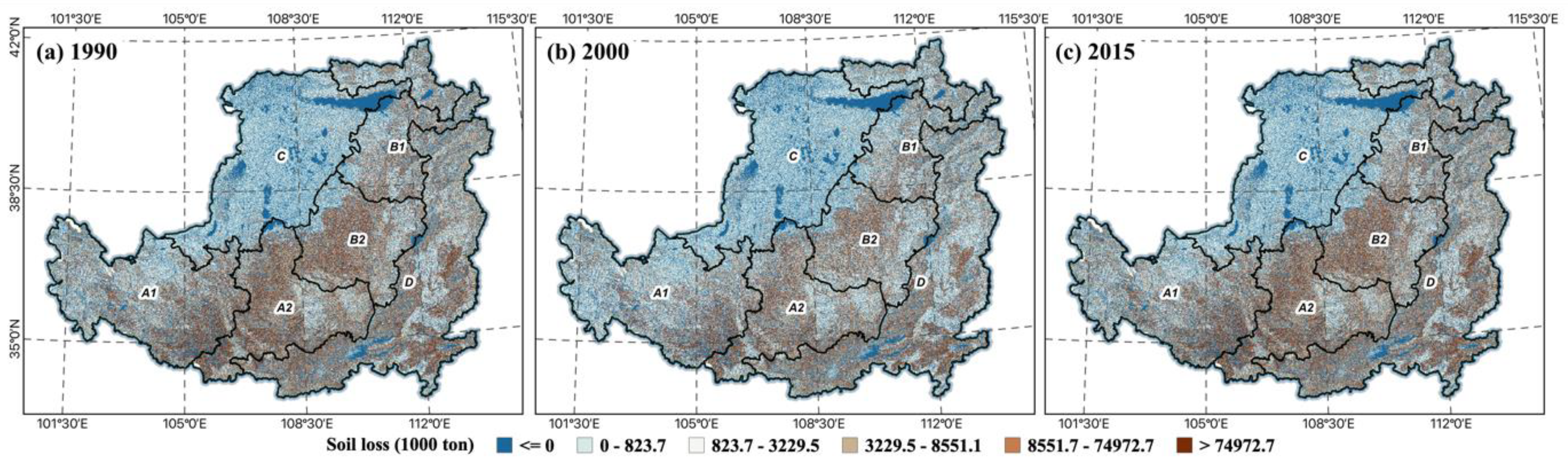
3.3.3. Soil Conservation Changes

The Loess Plateau was, at one point, the most severely eroded region in China due to its loose soil and heavy rainfall. Both soil loss and water yield exhibited comparable geographical trends. The soil loss and water yield increased gradually from the northwest to the southeast. In the northern and southwestern regions, soil losses increased, followed by a substantial decline in water yield. From 1990 to 2015, the total potential soil loss was reduced by approximately 41.3%, from 2.890 × 10 16   tons to 1.692 × 10 16 tons. Due to the regrowth of vegetation, soil and water conservation from 2000 to 2015 has improved greatly compared to 1990. During the period from 1990 to 2015, the spatial pattern was typically low in the north and high in the south. This suggests that the function of soil conservation is well-developed in regions with dense plant cover. In the eastern portion of Gansu Province, Northern Shaanxi Province, and Southern Ningxia Hui Autonomous Region, soil erosion was especially severe. In regions with less vegetation cover, the erosion problem is more significant. China had a population growth in the 1990s. To supply the need for food in Western China, massive deforestation and sloping land led to significant soil erosion in the Loess Plateau. Significant watersheds in China endured catastrophic floods in 1998, resulting in substantial human and monetary losses. As a result of this catastrophe, soil erosion has reached unparalleled levels of severity. In terms of ecological zones, soil erosion is most severe in the ditch areas of the Loess Hills (Figure 5). In addition, there are substantial variances in the soil conservation capacities of various land use types. Geographically, the possibility for total soil loss is greater in regions where farmland is concentrated. As a result of the execution of the GFGP, some agricultural land was turned into forest, resulting in a vastly increased capacity for soil conservation. In 2015, the overall potential soil loss has decreased in the majority of regions due to enhanced soil and water conservation capability.

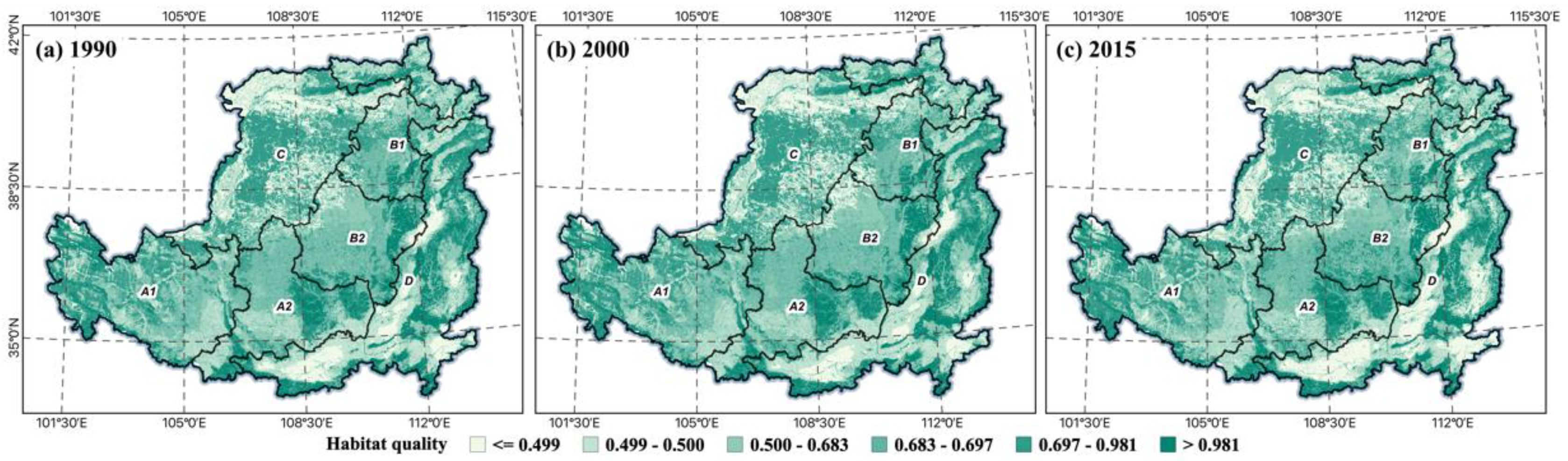
3.3.4. Habitat Quality Changes

Since the adoption of the GFGP in 1990, the average habitat quality in approximately 4.2% of cities and counties in the LP has increased between 1990 and 2015. In regions where soil loss is more severe, soil organic matter reduces concurrently with soil loss, biodiversity declines, and habitat quality worsens [58]. The results of habitat quality and land use have comparable spatial patterns throughout the LP (Figure 6). Forests and grasslands are primarily found in the southeast, where habitat quality is superior. In contrast, the majority of land use types in sandy and irrigated agricultural regions consist of underutilized and developed land with poorer habitat quality. Therefore, increased plant cover through the adoption of the GFGP may enhance habitat quality. The habitat quality of loess hills and ravines improved between 1990 and 2000. Additionally, the average habitat quality improved in the central region, where forest cover expanded. However, as a result of economic development and increased urbanization, built-up and undeveloped land areas in ecological zone D are expanding, resulting in a decline in habitat quality. The rise in habitat quality values generated by the expansion of forest and grassland areas as a result of the GFGP is somewhat compensated by the decline in habitat quality resulting from urbanization. Consequently, the average habitat quality in the LP changed somewhat between 2000 and 2015. In contrast, considerable changes occurred in regions where land use types altered. Forests and grasslands are the predominant habitat types with acceptable qualities. In contrast, the habitat quality of developed and undeveloped areas has diminished.

3.4. Trade-Offs/Synergies between ESs

Changes in correlations between ESs before and after the implementation of the GFGP were analyzed at the watershed scale in the LP from 1990 to 2015. Significant trade-offs/synergies relationships existed between each pair of ESs. Significant synergistic relationships existed between carbon storage, habitat quality, and soil conservation prior to GFGP implementation. Significant trade-offs also existed between water yield and other ESs (Table 3). The trade-off/synergy relationships between ESs have been strengthened after the GFGP implementation. For example, the Pearson coefficient between carbon storage and habitat quality increased from 0.741 in 1990 to 0.744 in 2015. Pearson coefficients between other ESs have increased to varying degrees. In addition to this, the negative correlation between water yield and each ES is increasing.
Spatially, this study used the root mean square error (RMSE) to express the trade-offs/synergies relationship between each pair of ESs at the spatial watershed scale (Figure 7). As seen in the figure, most pairs of ESs’ synergistic relationships in the LP have been strengthened after implementing the GFGP. The spatial characteristics are more evident for the three pairs of ESs, HQ and CS, HQ and WY, and HQ and SC. These three pairs of ecosystem trade-offs generally show lower values in the northern and southern parts and higher in the central part. The areas with high synergistic values are also where forest land is concentrated. As the area of forested land increases, the synergistic values of these pairs of ecosystem services also become more prominent. Thus, the correlation coefficient results and the spatial RMSE results show that the GFGP strengthens the synergy between most pairs of ESs.
This study counted the trade-offs/synergies relationships between each pair of ESs based on ecological zones. The results showed that after implementing GFGP, most of the synergistic relationships were enhanced, including HQ and SC, CS and HQ, CS and SC, SC and WY, and HQ and WY (Figure S2). Only one pair of ESs, the trade-off relationships between CS and WY had enhanced. The trade-offs/synergies relationships of HQ and SC results showed that the trade-off relationships of ESs in ecoregion A1 and A2 were enhanced in 2015. The rest pairs of the ESs in the ecological partitions showed enhanced synergistic relationships. The synergistic relationships between ESs in CS and HQ were increasing in all ecological partitions. Most of the ecological partitions in CS and SC showed enhanced synergistic relationships. Only B1 showed a slight enhancement in trade-off relationships between CS and SC. SC and WY was consistent with CS and SC results, which also showed enhanced trade-off relationships in ecological partition B1. HQ and WY showed little change in trade-offs/synergies relationships between ESs after implementing GFGP, and most of them were also synergistically enhanced. In contrast, the trade-off relationships between CS and WY had enhanced in all ecological zones in 2015.

3.5. Factors Influencing ESs Synergy

This study used a geographical detector to explore the spatial heterogeneity of trade-offs/synergies between ESs on the LP following the implementation of the GFGP, and the driving factors affecting them. The influence of each driver on the ESs trade-offs/synergies was determined by calculating the q-value of each driving factor (Table S3). The results indicate that topography and climate are important determinant variables explaining the synergetic relationships between ESs, while the influence of socioeconomic factors is relatively weak. According to the q-value results, for CS and HQ, CS and WY, and HQ and, DEM significantly explains these three pairs of ESs trade-offs/synergies relationships compared to other aspects. Their q-values were 0.114, 0.009, and 0.122, respectively, while the other three pairs of ecosystem services’ trade-offs/synergies were mainly influenced by rainfall, which affected their spatial distribution. The mean annual rainfall mainly explained the CS and SC, HQ and SC, and SC and WY trade-offs/synergies relationships. Their q-values are 0.041, 0.028, and 0.043, respectively. Heavy rainfall accelerates soil erosion and affects soil conservation as an ecosystem service function.
The geographical detector can also identify the interactions among the driving factors to assess a few factors. First, whether the driving factors, when acting together, increase or decrease the explanatory power of the trade-offs/synergies between ESs alternatively. Second, whether the effects of these driving factors on the trade-offs/synergies between ES are independent. The type of interaction was determined based on the q-value of the driver and interaction [59]. The results showed that the interaction factors of the dominant factors had interactive effects on the trade-offs between ESs, which showed non-linear enhancement and two-factor enhancement (Table 4). For CS and HQ and CS and WY, topography and rainfall interacted to produce non-linear enhancement effects. The interaction between rainfall and vegetation cover for HQ and SC also produced a non-linear enhancement effect. In addition, for CS and SC, HQ and WY, and SC and WY, the interaction of topography and rainfall factors produced a two-factor enhancement effect. In summary, the effects of each driver on ESs are not just a single independent superposition but a bi-factorial or non-linear enhancement effect.

4. Discussions

4.1. Implications

The results of NDVI trends in the LP during 1990–2015 show that the GFGP has changed the vegetation dynamics of the LP to a large extent. The greening areas of the LP have gradually expanded, especially in key counties, since the GFGP was implemented, from the initially densely distributed southeastern part to the northwestern part to the central part, such as Yulin City in Shaanxi Province. The vegetation cover of sandy and agricultural irrigation areas, where NDVI was relatively low, also gradually increased. Overall, the vegetation cover in most areas of the LP has been improved, and the ecological environment has been improved. These results are also consistent with the conclusions obtained from some previous studies. However, NDVI only reflects the dynamic changes in vegetation in general. NDVI changes are influenced by GFGP and natural factors, including rainfall and temperature, socio-economic factors including population growth, and specific errors in remote sensing images, all of which can lead to changes in NDVI. Therefore, it is not very comprehensive to measure the improvement of the GFGP on the ecosystem by only taking the change in one indicator of NDVI. We can consider the changes in various ESs in the LP before and after the implementation of GFGP to comprehensively analyze the contribution of GFGP to ecosystem restoration.
The majority of previous studies have also indicated that the execution of ecological restoration programs impacts ecosystem services. Most study scales concentrate on specific regions. To comprehend the intrinsic relationships between ecosystem services, however, it is inappropriate to generalize our conclusions to urban or county scales. Therefore, we must scale down to sub-watersheds. The results indicate that the implementation of GFGP has improved the LP’s ESs and has responded well to ecological degradation. Firstly, it changed the land use cover type, which may indirectly affect the ecological environment. After implementing GFGP, the cropland area decreased by 1946.48 km2, the forested increased by 113.45 km2, and the grassland increased by 1867.32 km2. These three categories are also the most dominant land use types in the LP. The area of forest land and grassland after the performance of GFGP far exceeds the amount before the implementation of GFGP. The GFGP can enhance ecosystem services by controlling trends in plant cover in land use. For instance, forest land is advantageous for the storage of carbon and the conservation of soil and water [60]. However, increased water use might also be a result of vegetation cover. The GFGP has increased vegetation cover, reduced surface runoff, and improved the physical properties of the soil. These changes have helped reduce soil erosion and maintain soil fertility after implementing the GFGP. Consequently, grassland can enhance other ecological functions while continuing to use less water [61]. Therefore, essentially the GFGP exerted positive effects on the ESs. Various ESs of the LP has been improved accordingly, and soil erosion has been slowed down. However, achieving synergies between ESs is a necessity for the success of future GFGP. The study results demonstrate the influence of ecological restoration projects on the trade-offs/synergies between ESs. Thus, we found out the enhancement of ecosystem services on the Loess Plateau, a crucial GFGP region. In addition, this can give decision-makers with policy suggestions for ecological restoration that are more supported by scientific evidence.
Most ESs have synergistic relationships with one another. From 1990 to 2015, the implementation of the GFGP compensated for the negative effects of external environmental pressures on CS, HQ, and SC, and greatly enhanced CS, HQ, and SC. This enhancement, however, came at the sacrifice of WY. The results of the geographical detector indicate enhanced interactive effects of climate and topography on trade-offs/synergies between ESs. If the benefits of one ecosystem service are maximized, this can lead to a significant decline in other ESs. Therefore, to better exploit the benefits of ESs, this study analyzed the relationships between pairs of ESs. Specifically, the results showed that the forest, and grassland increased significantly, and the vegetation cover increased after implementing GFGP compared with 1990. The associated carbon storage, habitat quality, and soil conservation ESs significantly increased in most areas of the LP. This suggests a synergistic relationship between them, and the implementation of GFGP has promoted this synergy. However, water consumption and evapotranspiration increased significantly due to the extensive planting of non-native monoculture vegetation in the GFGP areas [62]. Our results also showed that GFGP had a significant negative impact on water yield, so there may be a direct trade-off between regional water production and vegetation cover. This study confirms that GFGP brings ecological benefits while exacerbating regional water stress. Therefore, the improvement in soil erosion in the LP mainly results from the increased soil retention capacity and carbon sequestration.
The study results showed a significant increase in carbon sequestration and soil retention in most areas, indicating a synergistic relationship between these ESs. Contrary to previous studies, these studies concluded that trade-offs exist between ESs for the most part [63]. In order to restore the ecology and promote sustainable development, analysis to understand the relationship between ESs is essential for the future implementation of GFGP to protect the ecosystem. After the GFGP was implemented on the LP in 1999, the recovery of vegetation and the measurement of ESs indicate that the GFGP has effectively prevented further ecological degradation. The ultimate goal of policymakers has always been to maximize the benefits of ESs through effective policies [64]. Thus, the successful implementation of GFGP is an important guide for the scientific management of ecosystems and the improvement of ESs in developing countries and globally. However, as human activities intensify and ESs interact with each other, there is still some uncertainty about the future sustainability of the GFGP. It is essential to ensure that the food needs of the LP region can be secured and to do so in a planned manner to return cropland to forests. Moreover, the government should also focus on the shortage of water resources in the LP in implementing the GFGP. Therefore, without destroying vegetation and causing new soil erosion, the government needs to comprehensively consider the scope and intensity of the future GFGP and determine reasonable planting species.

4.2. Limitations

Most previous studies have relied only on single indicators to assess the effect of GFGP on ecosystem restoration, such as NDVI, NPP, or soil and water conservation. This study has extended the assessment of single indicators to a comprehensive evaluation using multiple ecosystem service functions representative of the study area and their trade-offs/synergies relationships, etc. However, ecosystems are complex internally. The improvement of ESs may be influenced by multiple aspects [8]. Understanding the connections between environmental services and influencing factors is essential for developing and enhancing ecosystem management methods. The intensity of human activity can alter land use patterns, hence influencing synergistic interactions between ecosystem services. In terms of natural conditions, vegetation recovery is frequently exposed to climate change pressures. Therefore, we can refine the various aspects of the factors that influence the interaction between ecosystem services in future research. By regulating the influencing factors or encouraging a specific service based on local conditions, managers can boost the production of numerous services and enhance the sustainability of development in this manner. So, it is challenging to measure the improvement of ESs comprehensively. Moreover, the process of ecological restoration requires long-term observation. There are data and spatial resolution limitations due to the data before the implementation of GFGP. Due to the limitation of remote sensing image acquisition, the data before the implementation of ecological restoration projects are difficult to obtain in high resolution. Therefore, it is difficult to compare the ecosystem services earlier with post-implementation of GFGP. The GFGP requires large amounts of money to compensate local farmers. This leads to overpayment for ESs regarding social costs. Therefore, as a next step, this study can take into account the quantitative assessment of this high economic input to ecological conservation. In addition to this, we can raise the awareness of farmers to protect the ecosystem through the local government’s publicity and then and then combine local field survey data and socio-economic factors before assessing their contribution to the ecological environment more comprehensively.

5. Conclusions

In this paper, we assessed the contribution of GFGP to ESs in the LP by analyzing the spatial and temporal changes in vegetation cover, land use changes, and improvements in ESs before and after the implementation of GFGP. In addition, we analyzed the trade-offs/synergies between ESs and the influencing factors. The main findings are as follows: the GFGP has resulted in a significant expansion of vegetation restoration in the LP, including an increase in the area of forest and grassland. Moreover, ESs were significantly improved after the implementation of GFGP. Carbon storage, habitat quality, and soil conservation showed synergistic relationships. Moreover, water yield showed a trade-off relationship with other ESs. Topography and climate are the two major factors affecting the degree of trade-offs/synergies between ESs. Therefore, analyzing the relationship between ESs can help develop sustainable ecological restoration projects.

Supplementary Materials

The following supporting information can be downloaded at: https://www.mdpi.com/article/10.3390/rs14235940/s1, Figure S1: Cropland use/cover change in the LP, 1990-2000 (a), 2000-2015 (b); Figure S2: Trade-offs/synergies change between ecosystem services in the LP, 1990, 2000 and 2015. Note: (a) HQ & SC; (b) CS & HQ; (c) CS & WY; (d) CS & SC; (e) SC & WY; (f) HQ & WY; Table S1: Land use transfer matrix in the LP, 1990-2000, 2000-2015 (Unit: km2); Table S2: The power of q for the 6 factors explaining the trade-offs/synergies between ecosystem services in the LP, 2015; Table S3: Interaction detection between ecosystem services in the LP, 2015. References [65,66,67,68,69,70,71,72] are cited in the supplementary materials.

Author Contributions

Conceptualization, X.D., A.C. and Z.Y.; methodology, Z.Y.; software, Z.Y.; validation, Z.Y.; formal analysis, Z.Y.; investigation, Z.Y..; resources, X.D.; data curation, Z.Y.; writing—original draft preparation, Z.Y.; writing—review and editing, A.C.; visualization, Z.Y.; supervision, X.D. and A.C.; funding acquisition, X.D. All authors have read and agreed to the published version of the manuscript.

Funding

This research was funded by the Strategic Priority Research Program of the Chinese Academy of Sciences (grant number XDA23070400).

Data Availability Statement

The data that support the findings of this study are available from the corresponding author, upon reasonable request.

Conflicts of Interest

The authors declare no conflict of interest.

References

  1. Daily, G.C. Introduction: What Are Ecosystem Services. In Nature’s Services: Societal Dependence on Natural Ecosystems; Island Press: Washington, DC, USA, 1997; p. 1. [Google Scholar]
  2. Bennett, E.M.; Peterson, G.D.; Gordon, L.J. Understanding relationships among multiple ecosystem services. Ecol. Lett. 2009, 12, 1394–1404. [Google Scholar] [CrossRef] [PubMed]
  3. Foley, J.A.; DeFries, R.; Asner, G.P.; Barford, C.; Bonan, G.; Carpenter, S.R.; Chapin, F.S.; Coe, M.T.; Daily, G.C.; Gibbs, H.K.; et al. Global Consequences of Land Use. Science 2005, 309, 570–574. [Google Scholar] [CrossRef] [Green Version]
  4. Fisher, B.; Turner, R.K.; Morling, P. Defining and classifying ecosystem services for decision making. Ecol. Econ. 2009, 68, 643–653. [Google Scholar] [CrossRef] [Green Version]
  5. Millennium Ecosystem Assessment. Ecosystems and Human Well-Being: Wetlands and Water; World Resources Institute: Washington, DC, USA, 2005. [Google Scholar]
  6. DeFries, R.S.; Ellis, E.C.; Chapin, F.S., III; Matson, P.A.; Turner, B.L., II; Agrawal, A.; Crutzen, P.J.; Field, C.; Gleick, P.; Kareiva, P.M.; et al. Planetary Opportunities: A Social Contract for Global Change Science to Contribute to a Sustainable Future. BioScience 2012, 62, 603–606. [Google Scholar] [CrossRef] [Green Version]
  7. Costanza, R.; D’Arge, R.; De Groot, R.; Farber, S.; Grasso, M.; Hannon, B.; Limburg, K.; Naeem, S.; O’Neill, R.V.; Paruelo, J.; et al. The value of the world’s ecosystem services and natural capital. Nature 1997, 387, 253–260. [Google Scholar] [CrossRef]
  8. Costanza, R.; de Groot, R.; Braat, L.; Kubiszewski, I.; Fioramonti, L.; Sutton, P.; Farber, S.; Grasso, M. Twenty years of ecosystem services: How far have we come and how far do we still need to go? Ecosyst. Serv. 2017, 28, 1–16. [Google Scholar] [CrossRef]
  9. Bai, Y.; Deng, X.; Jiang, S.; Zhang, Q.; Wang, Z. Exploring the relationship between urbanization and urban eco-efficiency: Evidence from prefecture-level cities in China. J. Clean. Prod. 2018, 195, 1487–1496. [Google Scholar] [CrossRef]
  10. Liu, X.; Wang, S.; Wu, P.; Feng, K.; Hubacek, K.; Li, X.; Sun, L. Impacts of Urban Expansion on Terrestrial Carbon Storage in China. Environ. Sci. Technol. 2019, 53, 6834–6844. [Google Scholar] [CrossRef]
  11. Wang, G.; Shi, R.; Mi, L.; Hu, J. Agricultural Eco-Efficiency: Challenges and Progress. Sustainability 2022, 14, 1051. [Google Scholar] [CrossRef]
  12. Ouyang, Z.; Zheng, H.; Xiao, Y.; Polasky, S.; Liu, J.; Xu, W.; Wang, Q.; Zhang, L.; Xiao, Y.; Rao, E.; et al. Improvements in ecosystem services from investments in natural capital. Science 2016, 352, 1455–1459. [Google Scholar] [CrossRef] [PubMed]
  13. Chen, Z.; Zhang, X. Value of ecosystem services in China. Chin. Sci. Bull. 2000, 45, 870–876. [Google Scholar] [CrossRef]
  14. Zhang, B.; Li, W.; Xie, G. Ecosystem services research in China: Progress and perspective. Ecol. Econ. 2010, 69, 1389–1395. [Google Scholar] [CrossRef]
  15. Deng, X.; Li, Z. Economics of land degradation in China. In Economics of Land Degradation and Improvement—A Global Assessment for Sustainable Development; Springer: Cham, Switzerland, 2016; pp. 385–399. [Google Scholar]
  16. Yu, Z.; Deng, X. Assessment of land degradation in the North China Plain driven by food security goals. Ecol. Eng. 2022, 183, 106766. [Google Scholar] [CrossRef]
  17. Zhao, X.; Wu, P.; Gao, X.; Persaud, N. Soil Quality Indicators in Relation to Land Use and Topography in a Small Catchment on the Loess Plateau of China. Land Degrad. Dev. 2015, 26, 54–61. [Google Scholar] [CrossRef]
  18. Ren, H.; Shen, W.J.; Lu, H.F.; Wen, X.Y.; Jian, S.G. Degraded ecosystems in China: Status, causes, and restoration efforts. Landsc. Ecol. Eng. 2007, 3, 1–13. [Google Scholar] [CrossRef]
  19. Zhang, L.; Wang, M.H.; Hu, J.; Ho, Y.S. A review of published wetland research, 1991–2008: Ecological engineering and ecosystem restoration. Ecol. Eng. 2010, 36, 973–980. [Google Scholar] [CrossRef]
  20. Wortley, L.; Hero, J.-M.; Howes, M. Evaluating Ecological Restoration Success: A Review of the Literature. Restor. Ecol. 2013, 21, 537–543. [Google Scholar] [CrossRef]
  21. Benayas, J.M.R.; Newton, A.C.; Diaz, A.; Bullock, J.M. Enhancement of Biodiversity and Ecosystem Services by Ecological Restoration: A Meta-Analysis. Science 2009, 325, 1121–1124. [Google Scholar] [CrossRef]
  22. Hua, F.; Wang, X.; Zheng, X.; Fisher, B.; Wang, L.; Zhu, J.; Tang, Y.; Yu, D.W.; Wilcove, D.S. Opportunities for biodiversity gains under the world’s largest reforestation programme. Nat. Commun. 2016, 7, 12717. [Google Scholar] [CrossRef] [Green Version]
  23. Geng, Q.; Ren, Q.; Yan, H.; Li, L.; Zhao, X.; Mu, X.; Wu, P.; Yu, Q. Target areas for harmonizing the Grain for Green Programme in China’s Loess Plateau. Land Degrad. Dev. 2020, 31, 325–333. [Google Scholar] [CrossRef]
  24. Shi, H.; Shao, M. Soil and water loss from the Loess Plateau in China. J. Arid. Environ. 2000, 45, 9–20. [Google Scholar] [CrossRef] [Green Version]
  25. Paoletti, E.; Schaub, M.; Matyssek, R.; Wieser, G.; Augustaitis, A.; Bastrup-Birk, A.M.; Bytnerowicz, A.; Günthardt-Goerg, M.; Müller-Starck, G.; Serengil, Y. Advances of air pollution science: From forest decline to multiple-stress effects on forest ecosystem services. Environ. Pollut. 2010, 158, 1986–1989. [Google Scholar] [CrossRef]
  26. Wang, J.; Peng, J.; Zhao, M.; Liu, Y.; Chen, Y. Significant trade-off for the impact of Grain-for-Green Programme on ecosystem services in North-western Yunnan, China. Sci. Total Environ. 2017, 574, 57–64. [Google Scholar] [CrossRef] [PubMed]
  27. Wu, X.; Wang, S.; Fu, B.; Liu, Y.; Zhu, Y. Land use optimization based on ecosystem service assessment: A case study in the Yanhe watershed. Land Use Policy 2018, 72, 303–312. [Google Scholar] [CrossRef]
  28. He, J.; Shi, X.; Fu, Y.; Yuan, Y. Evaluation and simulation of the impact of land use change on ecosystem services trade-offs in ecological restoration areas, China. Land Use Policy 2020, 99, 105020. [Google Scholar] [CrossRef]
  29. Liu, J.; Li, S.; Ouyang, Z.; Tam, C.; Chen, X. Ecological and socioeconomic effects of China’s policies for ecosystem services. Proc. Natl. Acad. Sci. USA 2008, 105, 9477–9482. [Google Scholar] [CrossRef] [Green Version]
  30. Deng, X.; Li, Z.; Gibson, J. A review on trade-off analysis of ecosystem services for sustainable land-use management. J. Geogr. Sci. 2016, 26, 953–968. [Google Scholar] [CrossRef] [Green Version]
  31. Chen, Y.; Wang, K.; Lin, Y.; Shi, W.; Song, Y.; He, X. Balancing green and grain trade. Nat. Geosci. 2015, 8, 739–741. [Google Scholar] [CrossRef]
  32. Wen, X.; Théau, J. Spatiotemporal analysis of water-related ecosystem services under ecological restoration scenarios: A case study in northern Shaanxi, China. Sci. Total Environ. 2020, 720, 137477. [Google Scholar] [CrossRef]
  33. Li, G.; Sun, S.B.; Han, J.C.; Yan, J.W.; Liu, W.B.; Wei, Y.; Lu, N.; Sun, Y.Y. Impacts of Chinese Grain for Green program and climate change on vegetation in the Loess Plateau during 1982–2015. Sci. Total Environ. 2019, 660, 177–187. [Google Scholar] [CrossRef] [PubMed]
  34. Fu, B.; Liu, Y.; Lü, Y.; He, C.; Zeng, Y.; Wu, B. Assessing the soil erosion control service of ecosystems change in the Loess Plateau of China. Ecol. Complex. 2011, 8, 284–293. [Google Scholar] [CrossRef]
  35. Eldridge, D.J.; Delgado-Baquerizo, M. Continental-scale Impacts of Livestock Grazing on Ecosystem Supporting and Regulating Services. Land Degrad. Dev. 2017, 28, 1473–1481. [Google Scholar] [CrossRef]
  36. Rodríguez, J.P.; Beard, T.D., Jr.; Bennett, E.M.; Cumming, G.S.; Cork, S.J.; Agard, J.; Dobson, A.P.; Peterson, G.D. Trade-offs across Space, Time, and Ecosystem Services. Ecol. Soc. 2006, 11, 28. [Google Scholar] [CrossRef] [Green Version]
  37. Zuo, L.; Gao, J. Investigating the compounding effects of environmental factors on ecosystem services relationships for Ecological Conservation Red Line areas. Land Degrad. Dev. 2021, 32, 4609–4623. [Google Scholar] [CrossRef]
  38. Roche, P.K.; Campagne, C.S. Are expert-based ecosystem services scores related to biophysical quantitative estimates? Ecol. Indic. 2019, 106, 105421. [Google Scholar] [CrossRef]
  39. Yang, M.; Gao, X.; Zhao, X.; Wu, P. Scale effect and spatially explicit drivers of interactions between ecosystem services—A case study from the Loess Plateau. Sci. Total Environ. 2021, 785, 147389. [Google Scholar] [CrossRef]
  40. Zhu, C.; Zhang, X.; Zhou, M.; He, S.; Gan, M.; Yang, L.; Wang, K. Impacts of urbanization and landscape pattern on habitat quality using OLS and GWR models in Hangzhou, China. Ecol. Indic. 2020, 117, 106654. [Google Scholar] [CrossRef]
  41. Wang, J.F.; Li, X.H.; Christakos, G.; Liao, Y.L.; Zhang, T.; Gu, X.; Zheng, X.Y. Geographical detectors-based health risk assessment and its application in the neural tube defects study of the Heshun region, China. Int. J. Geogr. Inf. Sci. 2010, 24, 107–127. [Google Scholar] [CrossRef]
  42. Zhang, Y.; Huang, M.; Lian, J. Spatial distributions of optimal plant coverage for the dominant tree and shrub species along a precipitation gradient on the central Loess Plateau. Agric. For. Meteorol. 2015, 206, 69–84. [Google Scholar] [CrossRef]
  43. Li, Z.; Zheng, F.L.; Liu, W.Z.; Jiang, D.J. Spatially downscaling GCMs outputs to project changes in extreme precipitation and temperature events on the Loess Plateau of China during the 21st Century. Glob. Planet. Chang. 2012, 82, 65–73. [Google Scholar] [CrossRef]
  44. Zhang, B.; Wu, P.; Zhao, X.; Wang, Y.; Gao, X. Changes in vegetation condition in areas with different gradients (1980–2010) on the Loess Plateau, China. Environ. Earth Sci. 2013, 68, 2427–2438. [Google Scholar] [CrossRef]
  45. Su, C.; Fu, B. Evolution of ecosystem services in the Chinese Loess Plateau under climatic and land use changes. Glob. Planet. Chang. 2013, 101, 119–128. [Google Scholar] [CrossRef]
  46. Li, J.; Ren, Z.; Zhou, Z. Quantitative analysis of the dynamic change and spatial differences of the ecological security: A case study of Loess Plateau in northern Shaanxi Province. J. Geogr. Sci. 2006, 16, 251–256. [Google Scholar] [CrossRef]
  47. Fu, B.; Chen, L. Agricultural landscape spatial pattern analysis in the semi-arid hill area of the Loess Plateau, China. J. Arid. Environ. 2000, 44, 291–303. [Google Scholar] [CrossRef] [Green Version]
  48. Sun, W.; Shao, Q.; Liu, J. Soil erosion and its response to the changes of precipitation and vegetation cover on the Loess Plateau. J. Geogr. Sci. 2013, 23, 1091–1106. [Google Scholar] [CrossRef]
  49. Yang, Y.F.; Wang, B.; Wang, G.L.; Li, Z.S. Ecological regionalization and overview of the Loess Plateau. Acta Ecol. Sin. 2019, 39, 7389–7397. [Google Scholar]
  50. Han, Z.; Song, W.; Deng, X.; Xu, X. Grassland ecosystem responses to climate change and human activities within the Three-River Headwaters region of China. Sci. Rep. 2018, 8, 9079. [Google Scholar] [CrossRef] [Green Version]
  51. Guan, D.; Gao, W.; Watari, K.; Fukahori, H. Land use change of Kitakyushu based on landscape ecology and Markov model. J. Geogr. Sci. 2008, 18, 455–468. [Google Scholar] [CrossRef]
  52. Wang, J.F.; Zhang, T.L.; Fu, B.J. A measure of spatial stratified heterogeneity. Ecol. Indic. 2016, 67, 250–256. [Google Scholar] [CrossRef]
  53. Wang, Y.; Wang, S.; Li, G.; Zhang, H.; Jin, L.; Su, Y.; Wu, K. Identifying the determinants of housing prices in China using spatial regression and the geographical detector technique. Appl. Geogr. 2017, 79, 26–36. [Google Scholar] [CrossRef]
  54. Egoh, B.; Reyers, B.; Rouget, M.; Richardson, D.M.; Le Maitre, D.C.; van Jaarsveld, A.S. Mapping ecosystem services for planning and management. Agric. Ecosyst. Environ. 2008, 127, 135–140. [Google Scholar] [CrossRef]
  55. Lu, N.; Fu, B.; Jin, T.; Chang, R. Trade-off analyses of multiple ecosystem services by plantations along a precipitation gradient across Loess Plateau landscapes. Landsc. Ecol. 2014, 29, 1697–1708. [Google Scholar] [CrossRef]
  56. Feng, X.M.; Sun, G.; Fu, B.J.; Su, C.H.; Liu, Y.; Lamparski, H. Regional effects of vegetation restoration on water yield across the Loess Plateau, China. Hydrol. Earth Syst. Sci. 2012, 16, 2617–2628. [Google Scholar] [CrossRef] [Green Version]
  57. Pimentel, D.; Harvey, C.; Resosudarmo, P.; Sinclair, K.; Kurz, D.; McNair, M.; Crist, S.; Shpritz, L.; Fitton, L.; Saffouri, R.; et al. Environmental and economic costs of soil erosion and conservation benefits. Science 1995, 267, 1117–1123. [Google Scholar] [CrossRef] [Green Version]
  58. Ju, H.; Zhang, Z.; Zuo, L.; Wang, J.; Zhang, S.; Wang, X.; Zhao, X. Driving forces and their interactions of built-up land expansion based on the geographical detector—A case study of Beijing, China. Int. J. Geogr. Inf. Sci. 2016, 30, 2188–2207. [Google Scholar] [CrossRef]
  59. Luo, Y.; Lü, Y.; Fu, B.; Zhang, Q.; Li, T.; Hu, W.; Comber, A. Half century change of interactions among ecosystem services driven by ecological restoration: Quantification and policy implications at a watershed scale in the Chinese Loess Plateau. Sci. Total Environ. 2019, 651, 2546–2557. [Google Scholar] [CrossRef] [PubMed] [Green Version]
  60. Feng, Q.; Zhao, W.; Hu, X.; Liu, Y.; Daryanto, S.; Cherubini, F. Trading-off ecosystem services for better ecological restoration: A case study in the Loess Plateau of China. J. Clean. Prod. 2020, 257, 120469. [Google Scholar] [CrossRef]
  61. Liu, B.; Xie, Y.; Li, Z.; Liang, Y.; Zhang, W.; Fu, S.; Yin, S.; Wei, X.; Zhang, K.; Wang, Z.; et al. The assessment of soil loss by water erosion in China. Int. Soil Water Conserv. Res. 2020, 8, 430–439. [Google Scholar] [CrossRef]
  62. Hu, Y.; Gao, M.; Batunacu. Evaluations of water yield and soil erosion in the Shaanxi-Gansu Loess Plateau under different land use and climate change scenarios. Environ. Dev. 2020, 34, 100488. [Google Scholar] [CrossRef]
  63. Xiao, Y.; Ouyang, Z.; Xu, W.; Xiao, Y.; Zheng, H.; Xian, C. Optimizing hotspot areas for ecological planning and management based on biodiversity and ecosystem services. Chin. Geogr. Sci. 2016, 26, 256–269. [Google Scholar] [CrossRef] [Green Version]
  64. Zhou, W.; Liu, G.; Pan, J.; Feng, X. Distribution of available soil water capacity in China. J. Geogr. Sci. 2005, 15, 3–12. [Google Scholar] [CrossRef]
  65. Gao, X.; Zhao, Q.; Zhao, X.; Wu, P.; Pan, W.; Gao, X.; Sun, M. Temporal and spatial evolution of the standardized precipitation evapotranspiration index (SPEI) in the Loess Plateau under climate change from 2001 to 2050. Sci. Total Environ. 2017, 595, 191–200. [Google Scholar] [CrossRef]
  66. Williams, J.R.; Greenwood, D.J.; Nye, P.H.; Walker, A. The erosion-productivity impact calculator (EPIC) model: A case history. Philos. Trans. R. Soc. London. Ser. B Biol. Sci. 1990, 329, 421–428. [Google Scholar] [CrossRef]
  67. Desmet, P.J.J.; Govers, G. A GIS procedure for automatically calculating the USLE LS factor on topographically complex landscape units. J. Soil Water Conserv. 1996, 51, 427. [Google Scholar]
  68. Chu, L.; Sun, T.; Wang, T.; Li, Z.; Cai, C. Evolution and Prediction of Landscape Pattern and Habitat Quality Based on CA-Markov and InVEST Model in Hubei Section of Three Gorges Reservoir Area (TGRA). Sustainability 2018, 10, 3854. [Google Scholar] [CrossRef] [Green Version]
  69. Tang, X.; Song, N.; Chen, Z.; Wang, J.; He, J. Estimating the potential yield and ETc of winter wheat across Huang-Huai-Hai Plain in the future with the modified DSSAT model. Sci. Rep. 2018, 8, 15370. [Google Scholar] [CrossRef] [PubMed] [Green Version]
  70. Liang, Y.; Hashimoto, S.; Liu, L. Integrated assessment of land-use/land-cover dynamics on carbon storage services in the Loess Plateau of China from 1995 to 2050. Ecol. Indic. 2021, 120, 106939. [Google Scholar] [CrossRef]
  71. Sun, X.; Lu, Z.; Li, F.; Crittenden, J.C. Analyzing spatio-temporal changes and trade-offs to support the supply of multiple ecosystem services in Beijing, China. Ecol. Indic. 2018, 94, 117–129. [Google Scholar] [CrossRef]
  72. Sharp, R.; Tallis, H.T.; Ricketts, T.; Guerry, A.D.; Wood, S.A.; Chaplin-Kramer, R.; Nelson, E.; Ennaanay, D.; Wolny, S.; Olwero, N.; et al. InVEST 3.8. 0 User’s Guide. In The Natural Capital Project; Stanford University: Stanford, CA, USA; University of Minnesota: Minneapolis, MN, USA; The Nature Conservancy: Arlington, VA, USA; World Wildlife Fund: Gland, Switzerland, 2020. [Google Scholar]
Figure 1. The land use map of the study area (a) and its location in China (b). Note: loess sorghum gully region A1; loess sorghum gully region A2; loess hilly and gully region B1; loess hilly and gully region B2; sandy land and agricultural irrigation region C; earth-rocky mountainous, and river valley plain region D. The key counties data were offered by the local government.
Remotesensing 14 05940 g001
Figure 2. Annual NDVI trend in the LP, 1990–2015 (a), 1990–2000 (b), 2000–2015 (c).
Remotesensing 14 05940 g002
Figure 3. Carbon storage change in the LP, 1990 (a), 2000 (b), 2015 (c).
Remotesensing 14 05940 g003
Figure 4. Water yield change in the LP, 1990 (a), 2000 (b), 2015 (c).
Remotesensing 14 05940 g004
Figure 5. Soil loss change in the LP, 1990 (a), 2000 (b), 2015 (c).
Remotesensing 14 05940 g005
Figure 6. Habit quality change in the LP, 1990 (a), 2000 (b), 2015 (c).
Remotesensing 14 05940 g006
Figure 7. Trade-offs/synergies change between ecosystem services in the LP, 1990, 2000, and 2015. Trade-offs/synergies between HQ & SC in 1990 (a), HQ & WY in 1990 (b), CS & HQ in 1990 (c), CS & WY in 1990 (d), CS & SC in 1990 (e), SC & WY in 1990 (f), HQ & SC in 2000 (g), HQ & WY in 2000 (h), CS & HQ in 2000 (i), CS & WY in 2000 (j), CS & SC in 2000 (k), SC & WY in 2000 (l), HQ & SC in 2015 (m), HQ & WY in 2015 (n), CS & HQ in 2015 (o), CS & WY in 2015 (p), CS & SC in 2015 (q), SC & WY in 2015 (r).
Remotesensing 14 05940 g007
Table 1. Methods for quantifying ecosystem services.
Ecosystem ServiceMathematical Expression
Water Yield Y ( x ) = { 1 A E T ( x ) P ( x ) } × P ( x )
Soil Conservation U S L E x = R x × K x × L S x × C x × P x
Habitat Quality Q x j = H x j × [ 1 ( D x j 2 D x j 2 + k 2 ) ]
Carbon Storage v a l u e _ s e q x = V s x q p t = 0 q p 1 1 ( 1 + r 100 ) t ( 1 + c 100 ) t
Table 2. Data sources and their spatial and temporal resolution.
DataData SourcesSpatial ResolutionTime Range
Land use mapsChinese Academy of Sciences Resource and Environmental Science Data Center (http://www.resdc.cn/ (accessed on 14 January 2022))1000 m1990–2015
Meteorological dataThe China Meteorological Sharing Service System (http://cdc.cma.gov.cn/ (accessed on 14 January 2022))1000 m1990–2015
Digital Elevation Model (DEM)Chinese Academy of Sciences Resource and Environmental Science Data Center (http://www.resdc.cn/ (accessed on 14 January 2022))30 m1990–2015
Soil propertyHarmonized World Soil Database (HWSD)1000 m1990–2015
GIMMS dataset (GIMMS3g) NDVIthe National Oceanic and Atmospheric Administration (NOAA) Advanced Very High-Resolution Radiometer (AVHRR)8000 m1990–2015
GDP (gross output
value/km2)
Chinese Academy of Sciences Resource and Environmental Science Data Center (http://www.resdc.cn/ (accessed on 14 January 2022))1000 m2015
Population pressure (Number/area)Chinese Academy of Sciences Resource and Environmental Science Data Center (http://www.resdc.cn/ (accessed on 14 January 2022))1000 m2015
Standardized Precipitation EvapotranspirationStandardized Precipitation Evapotranspiration Index (SPEI)1000 m2000–2015
Restricted soil root depth datathe World Soil Database and UNAOC (http://www.fao.org/3/X0490E/x0490e0b.htm (accessed on 14 January 2022))1000 m2015
Table 3. Pearson’s correlation coefficient between ecosystem services in the LP, 1990, 2000, 2015.
CS1990HQ1990SC1990WY1990
CS19901
HQ19900.741 **1
SC19900.864 **0.819 **1
WY1990−0.856 **−0.723 **−0.880 **1
CS2015HQ2015SC2015WY2015
CS20151
HQ20150.744 **1
SC20150.867 **0.824 **1
WY2015−0.871 **−0.723 **−0.895 **1
Note: ** Correlation is significant at the 0.01 level (2-tailed).
Table 4. Interaction detection between ecosystem services in the LP, 2015.
Pair of Ecosystem ServicesDominant FactorqDominant Interaction Factorq
CS and HQDEM0.114(PER) ∩ (CS and HQ)0.1471
CS and SCPER0.041(DEM) ∩ (CS and SC)0.0705
CS and WYDEM0.009(PER) ∩ (CS and WY)0.0259
HQ and SCPER0.028(NDVI) ∩ (HQ and SC)0.0461
HQ and WYDEM0.122(DEM) ∩ (HQ and WY)0.1502
SC and WYPER0.043(DEM) ∩ (SC and WY)0.0787
Publisher’s Note: MDPI stays neutral with regard to jurisdictional claims in published maps and institutional affiliations.

