

A VGGNet-Based Method for Refined Bathymetry from Satellite Altimetry to Reduce Errors
Abstract
:1. Introduction
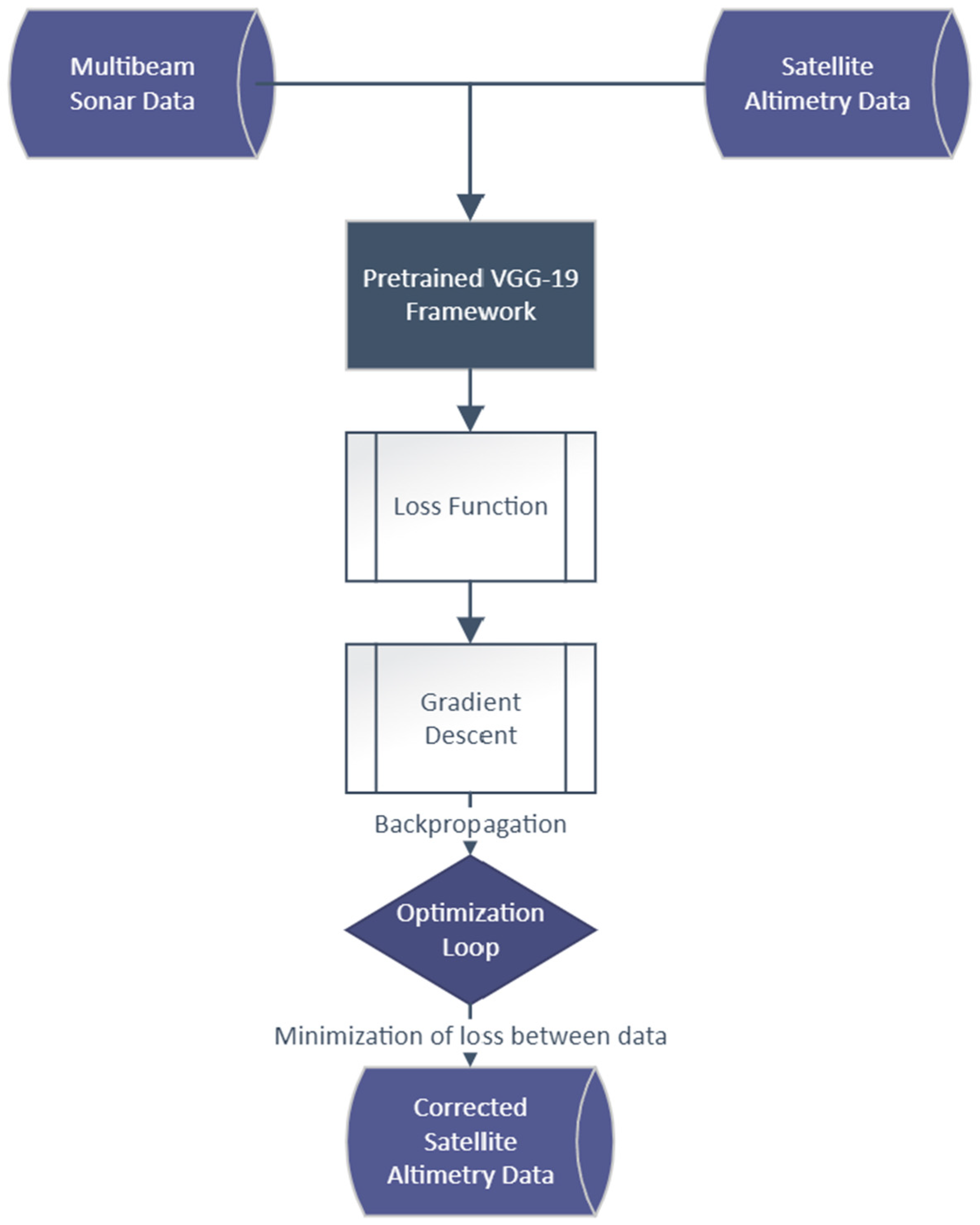
- A combination of high-spatial-resolution multibeam sonar-derived bathymetry (truth data) and high-coverage satellite altimetry-derived bathymetry (to-be-corrected data). This information is synthesized to obtain a corrected version of the latter, with the advantage of both.
- A convolutional neural network (CNN)-based VGGNet algorithm is for the first time proposed to compute the distance (loss) between the two inputs-to-be-corrected data and truth data, where the former is transformed by minimizing the distance between them with backpropagation, generating an image that best matches the latter.
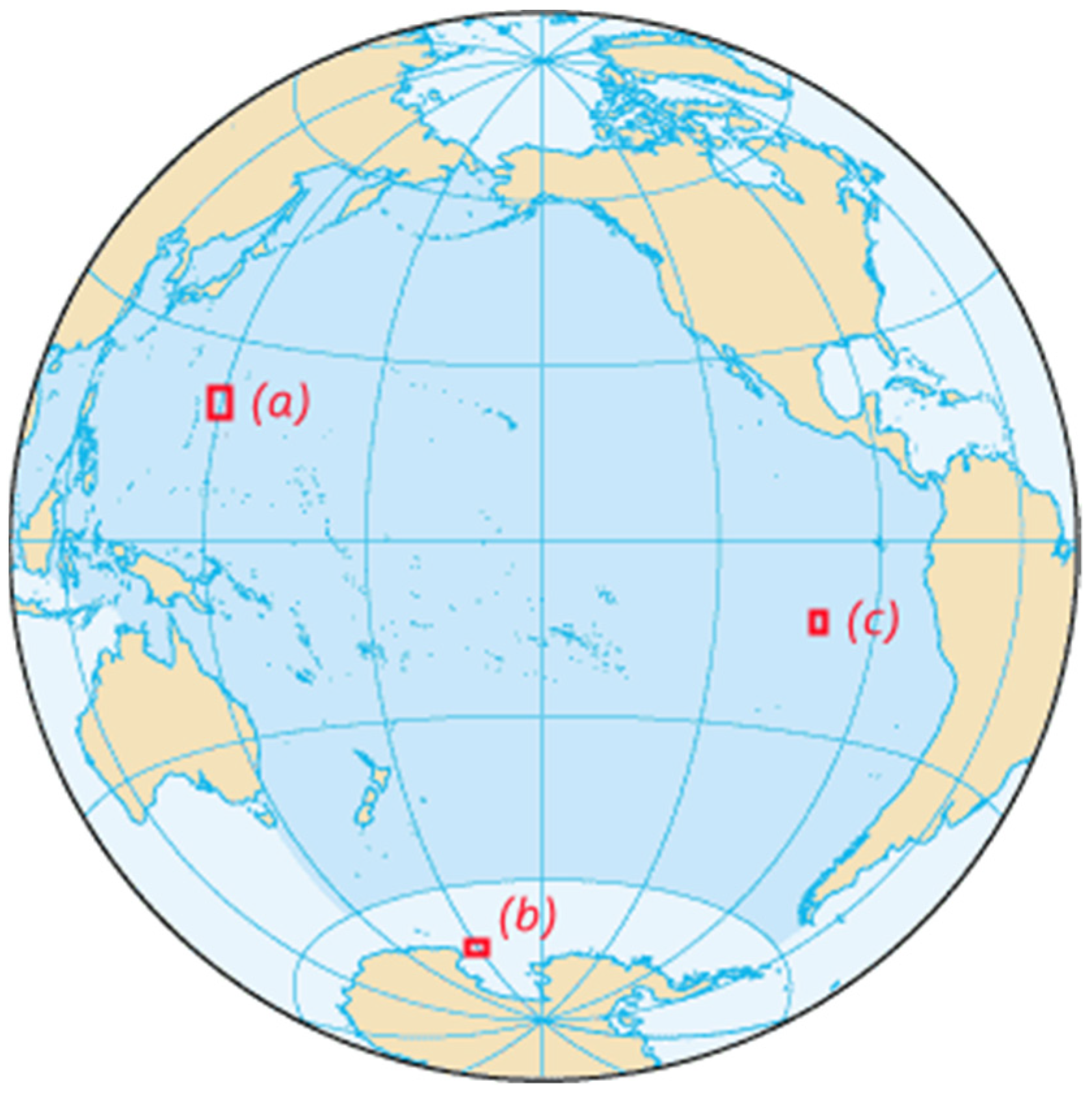
- Experiments are conducted in the West Pacific, Southern Ocean, and East Pacific, to test the algorithm’s performance, with the results showing that the improvement in computational precision can reach over 17% compared with previous research as far as we conclude.
2. Methodology and Data
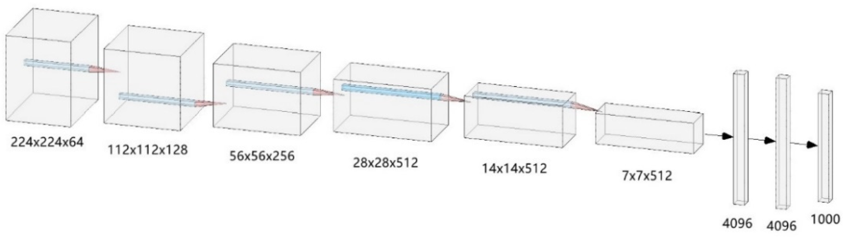
2.1. Framework of VGGNet
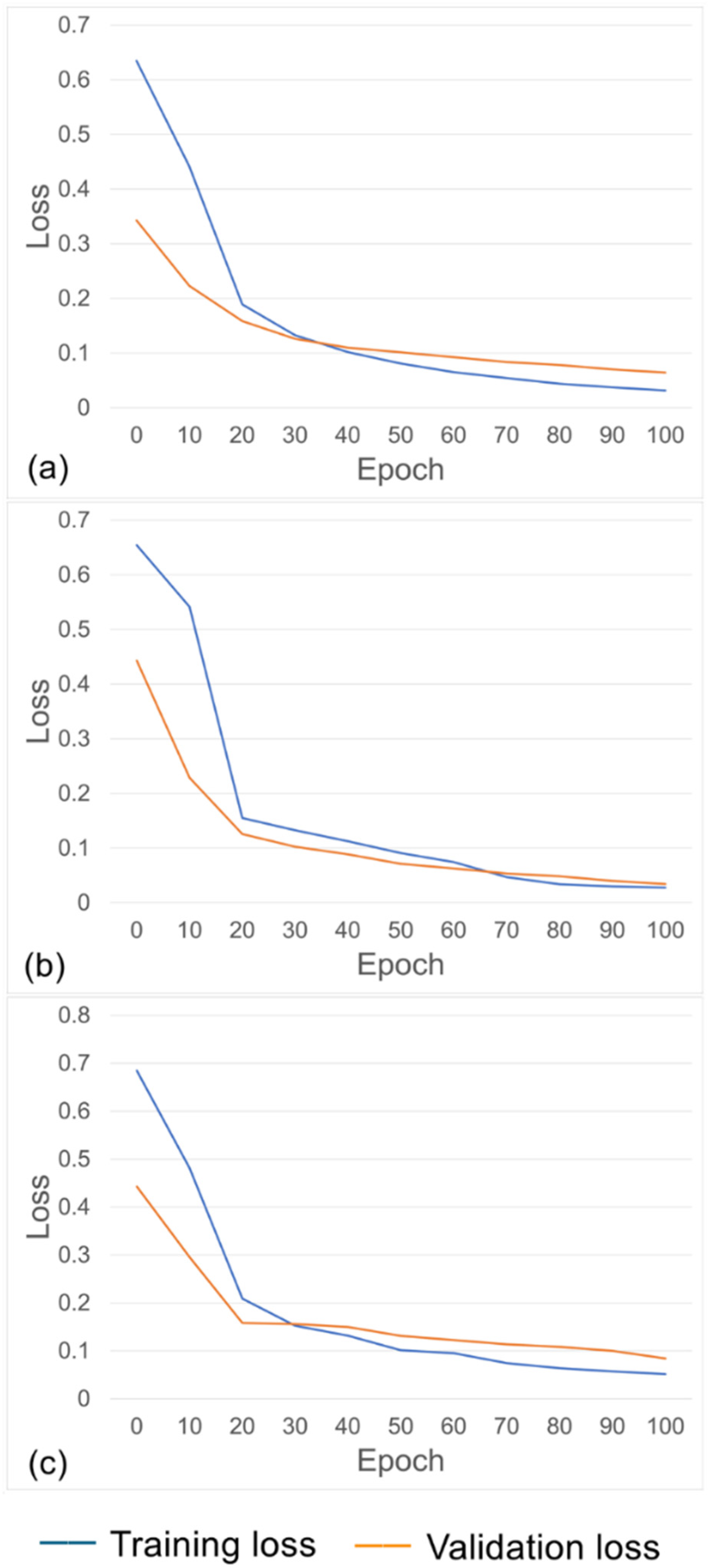
2.2. Model Training Steps
2.3. Experiment Data
3. Analysis of Results
4. Conclusions
Author Contributions
Funding
Data Availability Statement
Conflicts of Interest
References
- Fox, C.G.; Chadwick, W.W., Jr.; Embley, R.W. Detection of changes in ridge-crest morphology using repeated multibeam sonar surveys. J. Geophys. Res. Solid Earth 1992, 97, 11149–11162. [Google Scholar] [CrossRef]
- Wu, Y. A Study on Multi-Beam Sounding System Seafloor Tracking & Data Processing Techniques. Ph.D. Thesis, Harbin Engineering University, Harbin, China, 2001. [Google Scholar]
- Schimel, A.C.G.; Ierodiaconou, D.; Hulands, L.; Kennedy, D.M. Accounting for uncertainty in volumes of seabed change measured with repeat multibeam sonar surveys. Cont. Shelf Res. 2015, 111, 52–68. [Google Scholar] [CrossRef]
- Ma, J.; Jin, J.; Liu, Q. Multibeam Echosounder Versus Side Scan Object Detection: A Comparative Analysis. Hydrograph 2006, 26, 10–12. [Google Scholar] [CrossRef]
- Ji, X. Classification of Seabed Sediment and Terrain Complexity Based on Multibeam Data. Master’s Thesis, First Institute of Oceanography, Ministry of Natural Resources, Beijing, China, 2017. [Google Scholar]
- Pike, S.; Traganos, D.; Poursanidis, D.; Williams, J.; Medcalf, K.; Reinartz, P.; Chrysoulakis, N. Leveraging Commercial High-Resolution Multispectral Satellite and Multibeam Sonar Data to Estimate Bathymetry: The Case Study of the Caribbean Sea. Remote Sens. 2019, 11, 1830. [Google Scholar] [CrossRef] [Green Version]
- Cooper, I.; Hotchkiss, R.H.; Williams, G.P. Extending Multi-Beam Sonar with Structure from Motion Data of Shorelines for Complete Pool Bathymetry of Reservoirs. Remote Sens. 2021, 13, 35. [Google Scholar] [CrossRef]
- Pydyn, A.; Popek, M.; Kubacka, M.; Janowski, Ł. Exploration and reconstruction of a medieval harbour using hydroacoustics, 3-D shallow seismic and underwater photogrammetry: A case study from Puck, southern Baltic Sea. Archaeol. Prospect. 2021, 28, 527–542. [Google Scholar] [CrossRef]
- Li, J. Multibeam Survey Principles, Techniques and Methods; Ocean Press: Beijing, China, 1999. [Google Scholar]
- Coley, K. A Global Ocean Map is Not an Ambition, but a Necessity to Support the Ocean Decade. Mar. Technol. Soc. J. 2022, 56, 9–12. [Google Scholar] [CrossRef]
- Agrafiotis, P.; Karantzalos, K.; Georgopoulos, A.; Skarlatos, D. Correcting Image Refraction: Towards Accurate Aerial Image-Based Bathymetry Mapping in Shallow Waters. Remote Sens. 2020, 12, 322. [Google Scholar] [CrossRef] [Green Version]
- Liu, Y.M.; Deng, R.R.; Qin, Y.; Liang, Y.H. Data processing methods and applications of airborne LiDAR bathymetry. J. Remote Sens. 2017, 21, 982–995. [Google Scholar] [CrossRef]
- Parker, R.L. The Rapid Calculation of Potential Anomalies. Geophys. J. Int. 1972, 31, 447–455. [Google Scholar] [CrossRef]
- Dixon, T.H.; Naraghi, M.; McNutt, M.K.; Smith, S.M. Bathymetric prediction from Seasat altimeter data. J. Geophys. Res. Oceans 1983, 88, 1563–1571. [Google Scholar] [CrossRef]
- Smith, W.H.F.; Sandwell, D.T. Bathymetric prediction from dense satellite altimetry and sparse shipboard bathymetry. J. Geophys. Res. Solid Earth 1994, 99, 21803–21824. [Google Scholar] [CrossRef]
- Ramillien, G.; Cazenave, A. Global bathymetry derived from altimeter data of the ERS-1 geodetic mission. J. Geodyn. 1997, 23, 129–149. [Google Scholar] [CrossRef]
- Arabelos, D. On The Possibility to Estimate Ocean Bottom Topography from Marine Gravity and Satellite Altimeter Data Using Collocation. In Geodesy on the Move; Forsberg, R., Feissel, M., Dietrich, R., Eds.; Springer: Berlin/Heidelberg, Germany, 1998; Volume 117, pp. 105–112. [Google Scholar] [CrossRef]
- Calmant, S.; Baudry, N. Modelling bathymetry by inverting satellite altimetry data: A review. Mar. Geophys. Res. 1996, 18, 123–134. [Google Scholar] [CrossRef]
- Yeu, Y.; Yee, J.-J.; Yun, H.S.; Kim, K.B. Evaluation of the Accuracy of Bathymetry on the Nearshore Coastlines of Western Korea from Satellite Altimetry, Multi-Beam, and Airborne Bathymetric LiDAR. Sensors 2018, 18, 2926. [Google Scholar] [CrossRef] [PubMed] [Green Version]
- Brêda, J.P.L.F.; Paiva, R.C.D.; Bravo, J.M.; Passaia, O.A.; Moreira, D.M. Assimilation of Satellite Altimetry Data for Effective River Bathymetry. Water Resour. Res. 2019, 55, 7441–7463. [Google Scholar] [CrossRef]
- Wölfl, A.-C.; Snaith, H.; Amirebrahimi, S.; Devey, C.W.; Dorschel, B.; Ferrini, V.; Huvenne, V.A.I.; Jakobsson, M.; Jencks, J.; Johnston, G.; et al. Seafloor Mapping—The Challenge of a Truly Global Ocean Bathymetry. Front. Mar. Sci. 2019, 6, 283. [Google Scholar] [CrossRef] [Green Version]
- Sepúlveda, I.; Tozer, B.; Haase, J.S.; Liu, P.L.-F.; Grigoriu, M. Modeling Uncertainties of Bathymetry Predicted with Satellite Altimetry Data and Application to Tsunami Hazard Assessments. J. Geophys. Res. Solid Earth 2020, 125, 9. [Google Scholar] [CrossRef]
- Dierssen, H.M.; Theberge, A.E. Bathymetry: Assessment. In Coastal and Marine Environments, 2nd ed.; CRC Press: Boca Raton, FL, USA, 2020; pp. 175–184. [Google Scholar]
- Dettmering, D.; Ellenbeck, L.; Scherer, D.; Schwatke, C.; Niemann, C. Potential and Limitations of Satellite Altimetry Constellations for Monitoring Surface Water Storage Changes—A Case Study in the Mississippi Basin. Remote Sens. 2020, 12, 3320. [Google Scholar] [CrossRef]
- Wu, Z.; Yang, F.; Tang, Y. High-Resolution Seafloor Survey and Applications; Science Press: Beijing, China, 2021. [Google Scholar]
- Zhang, B.; Chen, Y.; Yuan, Y. PPP-RTK based on undifferenced and uncombined observations: Theoretical and practical aspects. J. Geod. 2019, 93, 1011–1024. [Google Scholar] [CrossRef]
- Zhang, B.; Hou, P.; Zha, J.; Liu, T. Integer-estimable FDMA model as an enabler of GLONASS PPP-RTK. J. Geod. 2021, 95, 91. [Google Scholar] [CrossRef]
- Mou, L.; Ghamisi, P.; Zhu, X.X. Deep Recurrent Neural Networks for Hyperspectral Image Classification. IEEE Trans. Geosci. Remote Sens. 2017, 55, 3639–3655. [Google Scholar] [CrossRef] [Green Version]
- Li, S.; Song, W.; Fang, L.; Chen, Y.; Ghamisi, P.; Benediktsson, J.A. Deep Learning for Hyperspectral Image Classification: An Overview. IEEE Trans. Geosci. Remote Sens. 2019, 57, 6690–6709. [Google Scholar] [CrossRef] [Green Version]
- Hong, D.; Gao, L.; Yao, J.; Zhang, B.; Plaza, A.; Chanussot, J. Graph Convolutional Networks for Hyperspectral Image Classification. IEEE Trans. Geosci. Remote Sens. 2021, 59, 5966–5978. [Google Scholar] [CrossRef]
- Girshick, R.; Donahue, J.; Darrell, T.; Malik, J. Rich Feature Hierarchies for Accurate Object Detection and Semantic Segmentation. In Proceedings of the 2014 IEEE Conference on Computer Vision and Pattern Recognition, Columbus, OH, USA, 24–27 June 2014. [Google Scholar] [CrossRef] [Green Version]
- Evans, M.C.; Ruf, C.S. Toward the Detection and Imaging of Ocean Microplastics with a Spaceborne Radar. IEEE Trans. Geosci. Remote Sens. 2022, 60, 4202709. [Google Scholar] [CrossRef]
- Gatys, L.A.; Ecker, A.S.; Bethge, M. A Neural Algorithm of Artistic Style. J. Vis. 2015, 16, 326. [Google Scholar] [CrossRef]
- Gatys, L.A.; Ecker, A.S.; Bethge, M.; Hertzmann, A.; Shechtman, E. Controlling Perceptual Factors in Neural Style Transfer. In Proceedings of the IEEE Conference on Computer Vision and Pattern Recognition, Honolulu, HI, USA, 22–25 July 2017. [Google Scholar] [CrossRef] [Green Version]
- Jena, B.; Kurian, P.J.; Swain, D.; Tyagi, A.; Ravindra, R. Prediction of bathymetry from satellite altimeter based gravity in the Arabian Sea: Mapping of two unnamed deep seamounts. Int. J. Appl. Earth Obs. Geoinf. 2012, 16, 1–4. [Google Scholar] [CrossRef]
- Jha, S.K.; Mariethoz, G.; Kelly, B.F.J. Bathymetry fusion using multiple-point geostatistics: Novelty and challenges in representing non-stationary bedforms. Environ. Model. Softw. 2013, 50, 66–76. [Google Scholar] [CrossRef]
- Moran, N.P. Machine Learning Model Selection for Predicting Global Bathymetry. Master’s Thesis, University of New Orleans, New Orleans, LA, USA, 2020. [Google Scholar]
- Ghorbanidehno, H.; Lee, J.; Farthing, M.; Tyler, H.; Darve, E.F.; Kitanidis, P.K. Deep learning technique for fast inference of large-scale riverine bathymetry. Adv. Water Resour. 2021, 147, 103715. [Google Scholar] [CrossRef]
- Krizhevsky, A.; Sutskever, I.; Hinton, G.E. ImageNet Classification with Deep Convolutional Neural Networks. In Proceedings of the 25th International Conference on Neural Information Processing Systems, Lake Tahoe, NV, USA, 3–6 December 2012. [Google Scholar] [CrossRef] [Green Version]
- Jia, Y.; Shelhamer, E.; Donahue, J.; Karayev, S.; Long, J.; Girshick, R.; Guadarrama, S.; Darrell, T. Caffe: Convolutional Architecture for Fast Feature Embedding. In Proceedings of the 22nd ACM International Conference, Orlando, FL, USA, 3–7 November 2014. [Google Scholar] [CrossRef]
- Simonyan, K.; Zisserman, A. Very Deep Convolutional Networks for Large-Scale Image Recognition. In Proceedings of the 3rd International Conference on Learning Representations, San Diego, CA, USA, 7–9 May 2015. [Google Scholar]
- Huo, G.; Wu, Z.; Li, J. Underwater Object Classification in Sidescan Sonar Images Using Deep Transfer Learning and Semisynthetic Training Data. IEEE Access 2020, 8, 47407–47418. [Google Scholar] [CrossRef]
- Islam, M.J.; Xia, Y.; Sattar, J. Fast Underwater Image Enhancement for Improved Visual Perception. IEEE Robot. Autom. Lett. 2020, 5, 3227–3234. [Google Scholar] [CrossRef] [Green Version]
- Schulz, M.-A.; Yeo, B.T.T.; Vogelstein, J.T.; Mourao-Miranada, J.; Kather, J.N.; Kording, K.; Richards, B.; Bzdok, D. Different scaling of linear models and deep learning in UKBiobank brain images versus machine-learning datasets. Nat. Commun. 2020, 11, 4238. [Google Scholar] [CrossRef] [PubMed]
- NOAA National Centers for Environmental Information: Multibeam Bathymetry Database (MBBDB). Available online: https://www.ncei.noaa.gov/access/metadata/landing-page/bin/iso?id=gov.noaa.ngdc:G01034 (accessed on 6 December 2021).
- NOAA National Geophysical Data Center: ETOPO1 1 Arc-Minute Global Relief Model. Available online: http://www.ncei.noaa.gov/access/metadata/landing-page/bin/iso?id=gov.noaa.ngdc.mgg.dem:316 (accessed on 6 December 2021).
- Reddi, S.J.; Kale, S.; Kumar, S. On the Convergence of Adam and Beyond. In Proceedings of the 6th International Conference on Learning Representations, Vancouver, BC, Canada, 30 April–3 May 2018. [Google Scholar]


| Coordinates of Center Point | Grid Resolution (m) | Data Size | Area (km2) | Depth Range (m) | |
|---|---|---|---|---|---|
| West Pacific | 19°N, 144°E | 103 | 12,624,868 | 133,937 | −8987–−369 |
| Southern Ocean | 71°S, 173°E | 93 | 5,097,104 | 43,700 | −4077–−211 |
| East Pacific | 27°S, 109°W | 93 | 9,135,007 | 78,318 | −3921–−1266 |
| Hyperparameters | Settings |
|---|---|
| Content layer | ‘conv4_2’ |
| Style layers | ‘conv1_1’, ‘conv2_1’, ‘conv3_1’, ‘conv4_1’, ‘conv5_1’ |
| Weights of loss at content layer | 1 |
| Weights of loss at style layers | 1, 1, 1, 1 |
| Weights among content, style, and total variation loss | 1 × 10⁻⁴, 1, 1 × 10⁻⁵ |
| Learning rate | starts at 10, linear decay over 100 iterations to 1 |
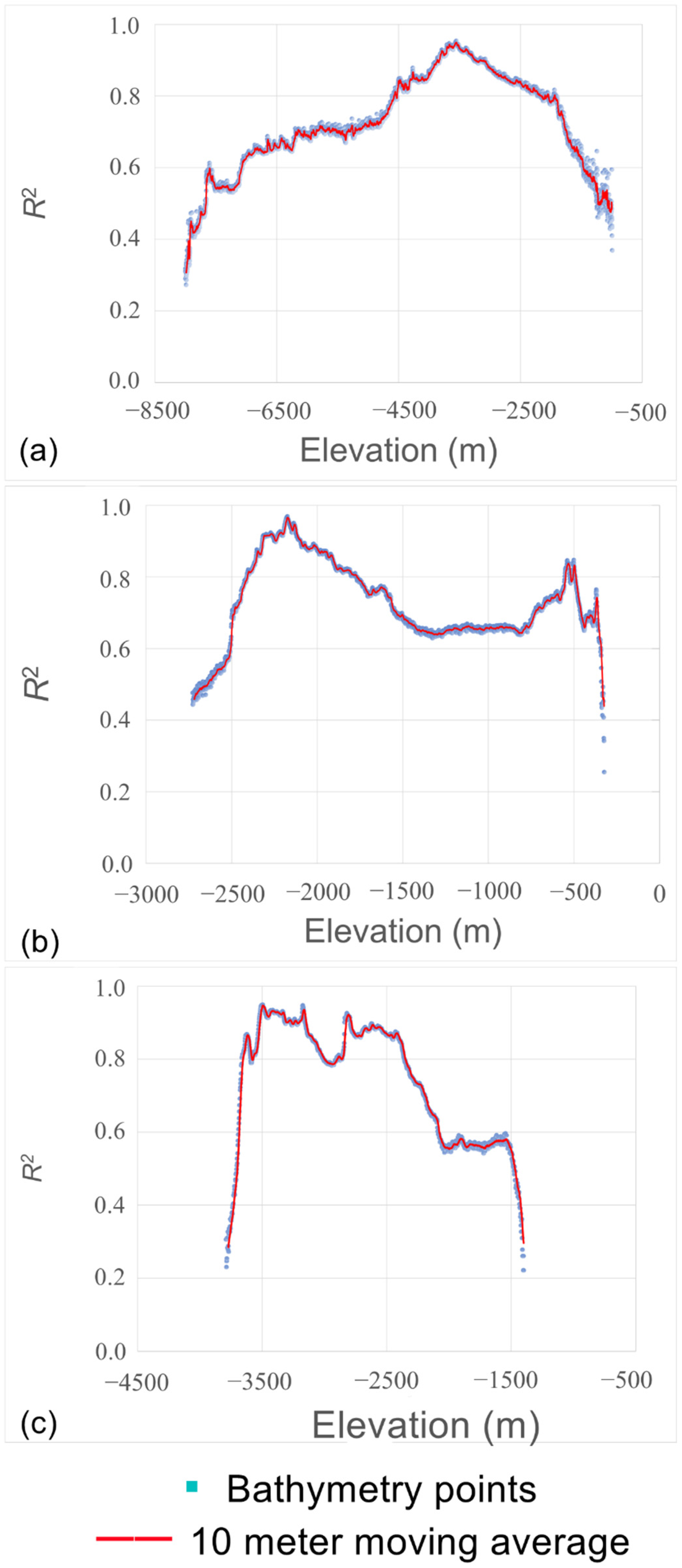
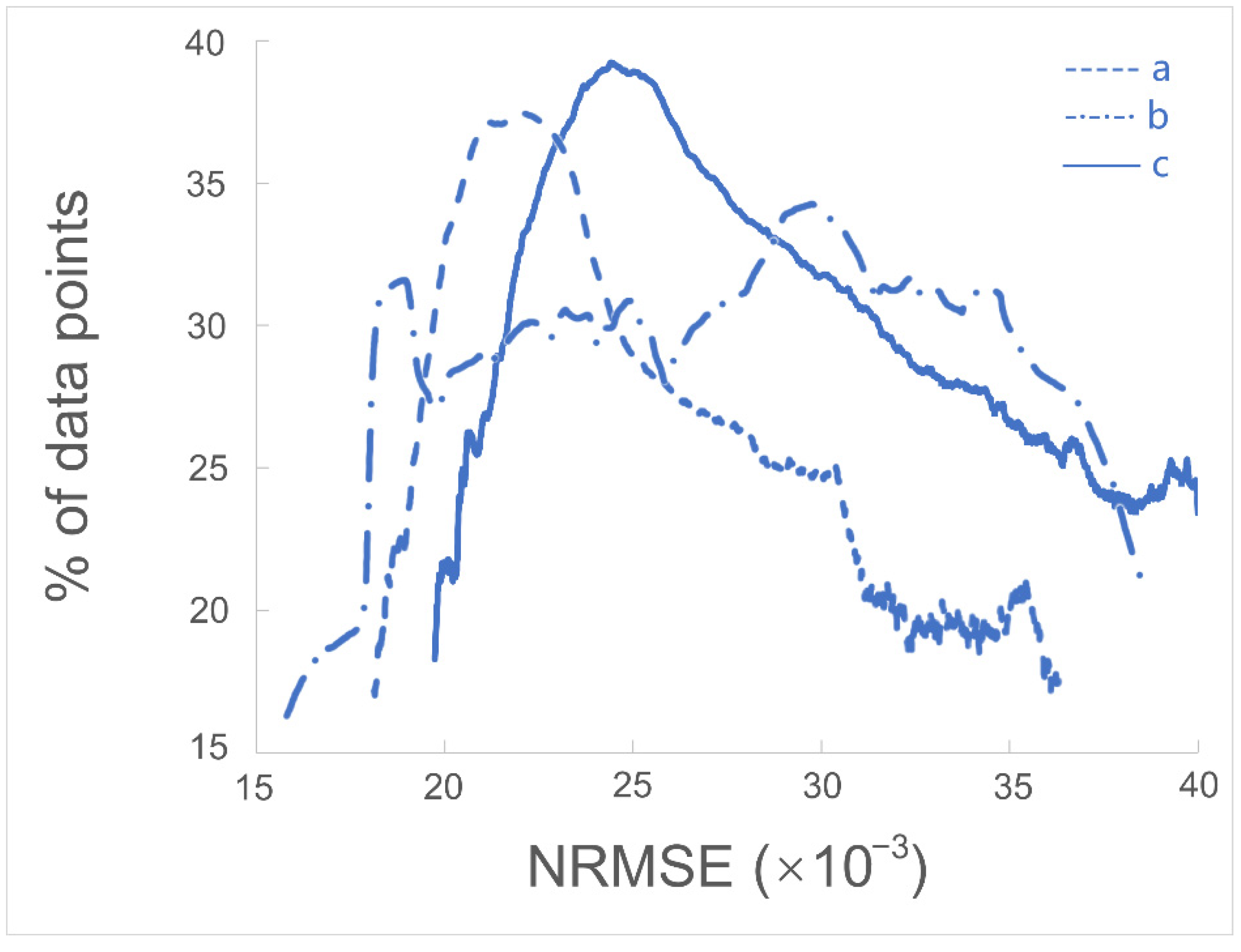
| R2 | RMSE (m) | NRMSE | |
|---|---|---|---|
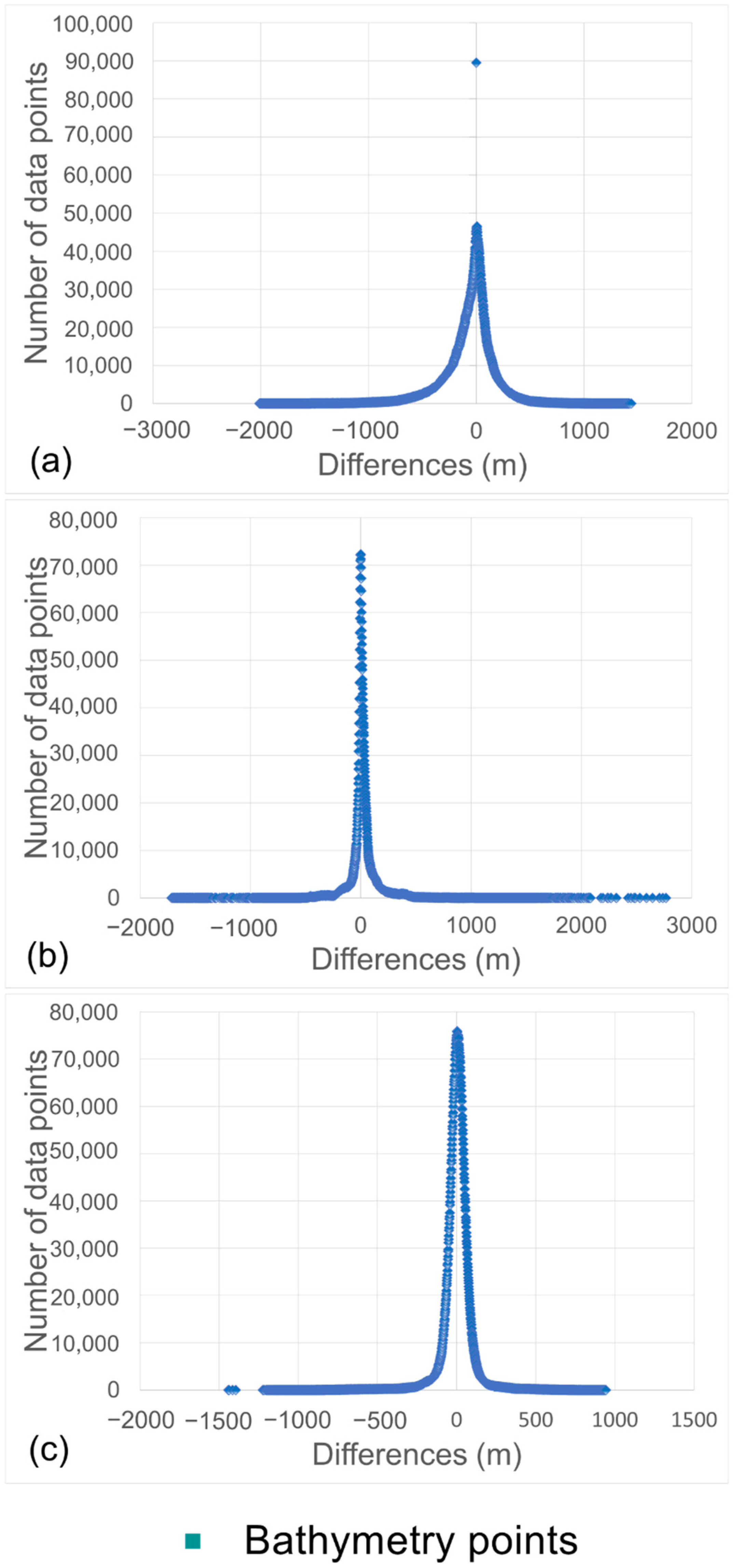
| West Pacific | 0.80 | 267 | 0.031 |
| Southern Ocean | 0.81 | 102 | 0.026 |
| East Pacific | 0.77 | 87 | 0.033 |
| 2% of Depth (%) | 1% of Depth (%) | |
|---|---|---|
| West Pacific | 67.25 | 45.73 |
| Southern Ocean | 76.19 | 60.34 |
| East Pacific | 68.30 | 41.55 |
Publisher’s Note: MDPI stays neutral with regard to jurisdictional claims in published maps and institutional affiliations. |
© 2022 by the authors. Licensee MDPI, Basel, Switzerland. This article is an open access article distributed under the terms and conditions of the Creative Commons Attribution (CC BY) license (https://creativecommons.org/licenses/by/4.0/).
Share and Cite
Chen, X.; Luo, X.; Wu, Z.; Qin, X.; Shang, J.; Li, B.; Wang, M.; Wan, H. A VGGNet-Based Method for Refined Bathymetry from Satellite Altimetry to Reduce Errors. Remote Sens. 2022, 14, 5939. https://doi.org/10.3390/rs14235939
Chen X, Luo X, Wu Z, Qin X, Shang J, Li B, Wang M, Wan H. A VGGNet-Based Method for Refined Bathymetry from Satellite Altimetry to Reduce Errors. Remote Sensing. 2022; 14(23):5939. https://doi.org/10.3390/rs14235939
Chicago/Turabian StyleChen, Xiaolun, Xiaowen Luo, Ziyin Wu, Xiaoming Qin, Jihong Shang, Bin Li, Mingwei Wang, and Hongyang Wan. 2022. "A VGGNet-Based Method for Refined Bathymetry from Satellite Altimetry to Reduce Errors" Remote Sensing 14, no. 23: 5939. https://doi.org/10.3390/rs14235939