Article

Temporal Subset SBAS InSAR Approach for Tropical Peatland Surface Deformation Monitoring Using Sentinel-1 Data

1
Faculty of Science and Engineering, Muroran Institute of Technology, Hokkaido 050-8585, Japan
2
Institute of Industrial Science, The University of Tokyo, Tokyo 153-8505, Japan
3
Research Organization of Aeronautics and Space, National Research and Innovation Agency (BRIN), Jakarta 10340, Indonesia
4
Research Organization for Earth Sciences and Maritime, National Research and Innovation Agency (BRIN), Jakarta 10340, Indonesia
5
Geospatial Information Agency (BIG), Bogor 16911, Indonesia
6
Center of Disaster Monitoring and Earth Observation, Universitas Negeri Padang, Padang 25173, Indonesia
7
Center for Environmental Remote Sensing, Chiba University, Chiba 263-8522, Japan
*
Author to whom correspondence should be addressed.
Remote Sens. 2022, 14(22), 5825; https://doi.org/10.3390/rs14225825
Submission received: 21 September 2022 / Revised: 7 November 2022 / Accepted: 7 November 2022 / Published: 17 November 2022
(This article belongs to the Special Issue Advances of SAR Data Applications)

Abstract

:
Tropical peatland in Southeast Asia has undergone rapid degradation and shows large subsidence due to oxidation and peat shrinkage. The measurement of those deformations is thus valuable for evaluating the peat condition and assessing peat restoration. The time series interferometric synthetic aperture radar (TInSAR), especially with the small baseline subsets (SBAS) method, is capable of measuring long-term deformation. However, the dynamic surface scatterers often change in tropical peatland, which degrades the coherent scatterer (CS) distribution density. This article presents a simple and efficient TInSAR approach that enhances the CS density under such dynamic surface scatter variation based on the SBAS method. In the presented approach, a long-time series of single-look complex images is separated into subsets, and deformation estimation is performed for each subset. The effectiveness of this simple solution was investigated by InSAR simulation and validated using SAR observation data. We applied the subset SBAS approach to the three-year Sentinel-1A C-band SAR dataset acquired over tropical peatland in Indonesia. The analyses showed an improved number of CSs for the introduced subset approach. We further introduce the color representation of CS temporal behavior per subset for visual interpretation of scatterer change.

1. Introduction

Peatland plays a critical role in carbon cycling, hydrology, and biodiversity and contributes to terrestrial carbon storage [1]. However, tropical peatland in Southeast Asia has undergone rapid degradation due to land conversion to agriculture, such as commercial oil palm and paper pulp tree plantations, since the 1970s [2,3]. Because deforestation associated with land transformation raises soil temperature and increases the number of drainage canals, a large area of tropical peatland has been drained, resulting in a decrease in the groundwater level (GWL) [4]. Such degradation accelerates peat microorganism oxidation (microbial decomposition) due to the increase in temperature and aeration together with a massive release of CO2 into the air and increasing peat fire risk. As the GWL decreases, tropical peatland subsides due to oxidation and peat shrinkage (consolidation and compaction). The peat subsidence associated with oxidation shows irreversible long-term behavior that usually continues for decades [5]. Moreover, peat shows short-term reversible deformation (peat oscillation) in response to climatic variations (i.e., changes in GWL) [6]. Therefore, measurement of both long-term and short-term peat surface deformation is valuable for evaluating the peat condition and assess peatland restoration [5].
Spaceborne synthetic aperture radar (SAR) is capable of regional-scale and regular data collection for surface deformation measurement and can reveal long-term dynamics using time-series interferometric SAR (TInSAR) [7]. TInSAR is a powerful geodetic technique to derive the temporal evolution of surface deformation. A series of repeated SAR images are taken into account in order to enable TInSAR to reduce atmospheric noise, orbital error, and spatio-temporal decorrelation. Some studies have used the TInSAR technique to monitor tropical peatland subsidence. Zhou et al. prepared a subsidence map for central Kalimantan in Indonesia derived from L-band ALOS PALSAR data and revealed restoration effects in the subsidence results [8]. Furthermore, Hoyt et al. computed large-scale (2.7-Mha) subsidence across Southeast Asian peatland from 2007 to 2011 with ALOS PALSAR data and quantified the widespread peat carbon loss due to oxidation [9]. The research in [10,11] revealed subsidence over peat-dominated Bengkalis Island in Indonesia using ALOS-2 PALSAR-2 data. Sentinel-1 C-band SAR data can also allow mapping of subsidence and were applied to tropical peatland in [10,12,13].
A number of TInSAR algorithms are available [7], and they can be categorized into three groups [14]. The first group is the persistent (point) scatterer (PS) approach that exploits continuously phased stable scatterers, usually corresponding most often to one dominant scatterer in the resolution cell [15,16]. The PS approach is therefore well suited for man-made targets in urban areas. The second one is the distributed scatterer (DS) approach, which relaxes the strict limit on the PS approach and treats a sufficiently large group of adjacent pixels sharing the same scattering mechanism using a redundant network of interferograms [14]. The DS approach can be applied to distributed natural areas, which are generally affected by high temporal decorrelation due to vegetation. The third one is a hybrid approach that accounts for both PS and DS [17,18].
Due to the great demand for deformation monitoring over natural distributed terrain, many DS approaches have been proposed so far, which can be categorized based on the interferogram network for deformation inversion. The first one uses all possible interferograms of employed SAR single-look complex (SLC) images (full network approach) [19] and estimates the deformation by the maximum likelihood estimator [18] or eigenvalue decomposition of the covariance matrix [20,21]. The second one uses part of all possible interferograms characterized by small spatio-temporal baselines, called small baseline subsets (SBAS), and estimates phase time series by least-squares (LS) estimation of a series of unwrapped phases [22,23]. Compared with the full interferogram network approach, SBAS is considered an efficient method for fast decorrelated pixels [24].
The adaptivity and accuracy of the TInSAR approach highly depend on the application and targets. When we aim to measure surface deformation over vegetated terrain, the SBAS seems to be one of the best solutions. Yunjun et al. proposed a new SBAS routine workflow with two improved phase unwrapping error correction algorithms [24]. This workflow selects coherent scatterers (CS) based on temporal coherence as a reliability measure to include not only decorrelation noise but also possible phase unwrapping errors. It was implemented as open-source software, named Miami InSAR time-series software in Python (MintPy) [24].
Here, we address monitoring peatland surface deformation in high temporal sampling. For this reason, we employed the Sentinel-1 C-band SAR satellite using the SBAS method. However, due to the dynamic surface scatterer changes, a direct adaptation of SBAS to tropical peatland is problematic. One example of the cause of such surface scatterer changes is a peat forest fire that transforms dense vegetation to bare ground or sparse vegetation. Such an event leads to an abrupt change in the scatterers. Other examples are farming or small-holder and industrial-plantation (e.g., oil palm and pulp tree) areas that exhibit a growth cycle, leading to evolutionary changes in vegetation scattering mechanisms.
As the duration of InSAR observations has increased over tropical peatland areas, some interferograms may suffer from the effects of inevitable surface scatterer changes. The abrupt and evolutionary changes in scatterers lead to decorrelation, systematically decreasing the number of CSs. Those scatterers may exhibit reasonable coherence during part of the time series. Such scatterers are referred to as temporary coherent scatterers (TCSs) [25]. The change time detection methods can identify coherent intervals. A number of methods have been proposed in the literature to statistically detect TCSs and identify coherent intervals [26,27,28,29,30]. Those TCS detection approaches were recently extended to the PS interferometry (PSI) framework. Hu et al. proposed a PSI method incorporating TCS [25]. Following this work, Nils et al. proposed integrating TCS into a PSI with iterative parameter estimation and phase unwrapping approaches. Although those developed algorithms provide an adaptive solution to scatterer change timing detection, it is computationally inefficient to process a large number of SLC images in deformation monitoring and is not tailored for the SBAS method. In addition, evolutional changes that occur in vegetated areas were not taken into account because previous studies considered only abrupt changes.
In the present work, we developed a simple and efficient approach based on SBAS to increase the density of CSs for tropical peatland deformation monitoring. The approach separates a long-time series of SAR images into several subsets. To our knowledge, incorporating the TCS concept into SBAS has not been discussed in any publications. Our intent is, therefore, to demonstrate the effectiveness of the temporal subset concept for SBAS and the applicability of the simple yearly based subset strategy based on the knowledge of seasonal and evolutional scatterer change. The solution was investigated by InSAR simulation and validated with tropical peatlands in Indonesia. We estimated a three-year tropical peatland surface deformation time series in the late 2010s (January 2018–January 2021) by our approach using Sentinel-1 C-band SAR data.

2. Dynamic Scatterer Changes in Tropical Peatland

2.1. Study Area

We measured peatland deformation in seven Sentinel-1A frames over Kalimantan (Indonesian part of Borneo Island) and Sumatra (Indonesia) from January 2018 until January 2021, as depicted by black rectangles in Figure 1. Those seven frames overwrap six Indonesian provinces: (1) Central Kalimantan, (2) South Kalimantan, (3) West Kalimantan, (4) Riau, (5) Jambi, and (6) South Sumatra. Peatlands on both islands are generally dome-shaped and restricted to lowlands, with elevations of less than 50 m above sea level [31], distributed over coastal regions. For the purpose of visualizing the study area, we display Landsat 8 true color optical images (RGB: bands 4, 3, and 2) of each frame in Figure 2, where those are the median images of two-year composite data (January 2018–January 2020) processed on Google Earth Engine (GEE).
The precipitation variability in Indonesian peatland is strongly affected by the El Niño–Southern Oscillation [32] and Indian-Ocean dipole (IOD) [33]. El Niño (warmer sea surface temperature in the Eastern Equatorial Pacific) and positive IOD (warmer sea surface temperature in the western Indian Ocean) events cause rain deficits during the dry season in Indonesia from May until October, leading to a decrease in GWL and an increase in forest fires, followed by haze pollution, carbon emissions, and subsidence. A positive IOD began around May 2019 and peaked around October 2019 during the observation period [34].
Figure 3a reveals the time series of rainfall and GWL at Palangka Raya city within Frame 1. We display the estimated GWL based on the procedure proposed by Takeuchi et al. [35,36]. The GWL is estimated by a modified Keetch-Byram drought index using satellite-based remote sensing products, including the Global Satellite Map of Precipitation (GSMaP), for daily rainfall r day (mm/day) and annual rainfall r year (mm/year), as well as the Advanced Himawari-8 Imager for maximum daily land surface temperature ( L S T max ). The rainfall time series in Figure 3a is derived from GSMaP products. In addition, we display in Figure 3b the number of fire hotspots per day produced by the MODIS Collection 6 active fire/thermal hotspot products, which were downloaded from NASA’s Fire Information for Resource Management System. We only use the fire hotspot data with a confidence level of 80% distributed across Indonesia. Figure 3 indicates that the GWL decrease during the dry season in 2019 was more severe and shows the highest number of fire hotspots during this time due to the positive IOD. Figure 3 also shows the clear seasonal temporal trend of GWL (rainfall) and fire hotspots in Indonesia.

2.2. Dynamic Scatterer Changes

The massive fire events in Figure 3b in the study area modified the peat surface conditions. As an example of surface change by fire in 2019, we show normalized difference vegetation index (NDVI) images of the east part of Jambi city within Frame 6 (latitude/longitude: −1.63/103.94) for 2018, 2019, and 2020 in Figure 4a–c, where the NDVI shows a higher value for dense vegetation cover. Each NDVI is computed using a mean of the yearly composite of Sentinel-2 optical images to mitigate cloud effects as much as possible, and processed on GEE. Figure 4a–c show a significant decrease in the NDVI from 2019 to 2020, which was caused by vegetation loss due to fire events during the dry season in 2019. The mean values of the NDVI within the red polygons in Figure 4a–c are 0.56, 0.56, and 0.39 for 2018, 2019, and 2020, respectively.
We further investigated the temporal SAR phase response in the fire-burned area of the red polygons in Figure 4c. To quantify the temporal phase stability (signal similarity between adjacent SLC images in the temporal domain), we measured spatial coherence, because it shows good correlation with NDVI [37], defined as
γ sp = s j s j + 1 * s j s j * s j + 1 s j + 1 * , j = 1 , , N 1
where s j (reference image) and s j + 1 (secondary image) are complex values corresponding to the same pixel forming an interferogram and indicates the ensemble averaging with the assumptions of stationarity and the ergodicity performed by spatial averaging. In Figure 5a, we show the spatial coherence time series derived by the adjacent co-registered SLC images (e.g., the result on 17 January is estimated by images observed on 5 January and 17 January with a shortest temporal baseline of 12 days). Those values are averaged over the red polygons shown in Figure 4a–c. Figure 5a clearly shows an abrupt coherence increase from around Sepetember 2019. Derived mean coherence values for each year are 0.69, 0.74, and 0.93 for 2018, 2019, and 2020, respectively. In the C band, high temporal decorrelation is expected over the vegetation area due to the higher variation in the motion of vegetation [38]. The abrupt coherence changes in Figure 5a indicate that the fire event in Jambi modified surface scatterers from vegetation to bare peatland. Note that a coherence fluctuation given in the results might be caused by a surface reflectance difference between two SAR images due to rainfall.
Oil palm plantation fields in West Kalimantan (latitude/longitude: −0.10/10.73) are another example of a change in scattering phenomena during observation. Figure 4d–f shows the yearly NDVI images for palm plantations of West Kalimantan in Frame 4. Mean NDVI values computed for the red polygons in Figure 4d–f are 0.50, 0.60, and 0.65 for 2018, 2019, and 2020, respectively. As mean NDVI values show an increasing trend, the growth of oil palm plantations and physical morphology changes in height and leaf structure are expected. The spatial coherence temporal behavior was also investigated and shown in Figure 5b, where those values are averaged over the red polygons in Figure 4d–f. The result reveals a decreased evolutional coherence trend, where the coherence drops from January 2019 and becomes gradual from January 2020. Consequently, the mean coherence in 2020 is 0.46, while those in 2018 and 2019 show high and moderate coherence values of 0.84 and 0.68, respectively.

3. Methodology

3.1. Time Series InSAR Processing

We processed three years of Sentinel-1A SLC data (C-band center frequency: 5.405 GHz) from January 2018 to January 2021 with 12-day intervals. The observation mode was an interferometric wide swath mode achieved by terrain observation by progressive scan [39]. We used vertical-vertical polarization in this study. To generate co-registered and phase-unwrapped interferogram stacks, we employed the stack sentinel processor in ISCE2 (https://github.com/isce-framework/isce2 (accessed on 2 August 2021)) [40]. A network-based enhanced spectral diversity approach was applied to Sentinel-1A images in ISCE2 for high-precision co-registration of SLC images [40]. For interferogram generation, we used a sequential interferogram network that pairs interferograms with their three nearest neighbors forward in time. An example of an interferogram network for Frame 3 is shown in Figure 6. Although this network with three nearest neighbors results in a 36-day maximum temporal baseline for a 12-day interval, some of our interferograms are paired with a 48-day temporal baseline due to missing SLC images.
We then performed multi-looking for each interferogram by 23 in the range (~100-m resolution) and 7 in the azimuth direction (~100 m resolution), and applied the Goldstein filter with a strength of 0.5. At the last stage of the stack sentinel processor, the SNAPHU algorithm was applied for phase unwrapping [41]. MintPy further processed a stack of phase-unwrapped interferograms generated by ISCE2 to produce a deformation time series.
For our processing, a reference point (point with known deformation) was set at Global Navigation Satellite System (GNSS) observation positions installed by the Geospatial Information Agency (BIG) of Indonesia [42]. The positions of this GNSS station are displayed as white circles in Figure 1. Therefore, all deformation values are referenced to a selected GNSS location. When a small deformation was found at some GNSS sensors, we subtracted the deformation at the GNSS sensor from the estimated time series deformation values of the corresponding InSAR frame. Because Frame 2 does not contain a GNSS station, we set a reference point at Sampit city (latitude/longitude: −2.54/112.96) in Central Kalimantan for Frame 2, assuming no deformation at Sampit city during the observation period.
Considering that M interferograms are generated by N SAR images, the i-th generated phase-unwrapped interferogram for each pixel can be modeled as
Δ ϕ i = Δ ϕ defo i + Δ ϕ APS i + Δ ϕ topo i + Δ ϕ res i + 2 π n amb i ,   i = 1 , . , M  
where Δ ϕ defo i denotes the phase difference due to deformation, Δ ϕ APS i denotes the atmospheric phase screen (APS) caused by temporal changes in tropospheric refractivity, Δ ϕ topo i denotes the residual topographic phase due to digital elevation model error, Δ ϕ res i denotes decorrelation phase noise, and n amb i denotes the integer phase ambiguity due to phase unwrapping error. MintPy further corrected the phase unwrapping error, atmospheric phase Δ ϕ APS i , and topographic phase error Δ ϕ topo i to precisely estimate the deformation phase term.
For spatio-temporal phase unwrapping, we applied two types of methods in MintPy: (1) the bridging method and (2) the phase closure method, both proposed in [24]. The bridging algorithm aims to estimate the integer phase ambiguity between “reliable regions” (one of the outcomes from SNAPHU [41]), which are a group of pixels believed to be free of relative local unwrapping errors [24]. This algorithm spatially corrects phase unwrap error based on the assumption that the phase difference between two reliable regions is less than π rad. In the temporal domain, the phase closure method estimates the integer phase offset based on the consistency of triplets of the interferometric phase.
After phase unwrap error correction, the interferometric phase in matrix form for each pixel can be given as
Δ ϕ = A · ϕ + Δ ϕ res ,  
where Δ ϕ is the [M × 1] vector of the interferometric phase, A is the [M × ( N-1)] design matrix, ϕ is [(N-1) × 1] vector of raw phase ( ϕ 2 ,   ϕ 3 , . , ϕ N ), and Δ ϕ res is the [M × 1] vector of the residual phase. Note that the initial phase ϕ 1 is removed from the system in (3) so that all raw phase values become relative measures referenced to ϕ 1 . The system in (3) is solved by weighted least-squares (WLS) solution, and the raw phase time series can be given by
ϕ ^ = A T · W · A 1 A T · W · Δ ϕ ,  
where W is an [M × M] square diagonal matrix that contains the inverse of the phase variance W = diag 1 / σ Δ ϕ 1 2 , 1 / σ Δ ϕ 2 2 , . . , 1 / σ Δ ϕ M 2 [43]. The quality of the inverted phase is then evaluated by the temporal coherence lying in the interval (0, 1) defined in each pixel as
γ tp = 1 M I T e j Δ ϕ A ϕ ^ ,  
where I is an [M × 1] identity matrix. Note that the decorrelation noise, residual phase unwrapping error, and phase contribution due to changes in scatterer properties (e.g., soil moisture) will degrade the γ tp . The pixels with γ tp higher than the predefined threshold of 0.65 were selected as CSs in our processing. Note that this threshold value was empirically determined in this study.
The nuisance terms of atmospheric phase error and topographic phase error are included in the derived raw phase time series in (4), which need further compensation. Global Atmospheric Models were used to estimate the atmospheric phase delay using re-analysis ERA5 data [44]. The residual topographic phase was corrected by the method in [45]. Once those nuisance terms were corrected, we obtained compensated raw phase time series vector ϕ ^ comp , which is expressed as the sum of the deformation phase vector ϕ defo and residual phase error vector ϕ res .
Finally, line-of-sight (LOS) deformation d LOS was converted into vertical deformation d v by d v = d LOS cos θ inc , where d LOS = λ 4 π ϕ ^ comp and θ inc denotes the incidence angle.

3.2. Temporal Subset SBAS Processing

We found a dynamic change in surface scatterers over the study area, mainly due to seasonal massive fire events and vegetation growth. As the observation period progresses, inevitable changes in scatterers are likely included in a series of SAR images. Such scatterer changes modify the noise level; hence, both decorrelated and less-decorrelated terms exist during the observation period, showing limited intervals of phase stability. In this case, although high phase stability was found in a specific period, the part of the data with high decorrelation would have degraded the overall γ tp . Consequently, such pixels were often rejected as CS when the whole datasets were simultaneously processed, leading to a spatially sparse density of deformation monitoring. The possible solution to this problem is to separate a series of SAR data into decorrelated and less-decorrelated periods, followed by evaluating γ tp for each separate data series. The timing of separation and the number of subsets highly depend on the pixels. A pixel-based adaptive approach can be considered; however, it carries a high computational burden because it evaluates each pixel. In this study, we applied the same data separation criterion to all the pixels, that is, the subset separation timing and the number of subsets were identical for all pixels.
After subset separation, interferograms were formed by SLC images of the corresponding subset through a sequential network. In our case, a stack of co-registered unwrapped interferograms was first generated, then the interferograms corresponding to the subset’s SLC images were extracted. Figure 6 schematically demonstrates this approach in the case of subsets divided by year. Subsequently, the WLS inversion was repeated for each subset. The temporal coherence of the k-th subset is given as
γ tp k = 1 M Ω I k T e j Δ ϕ k A k ϕ k ^ ,   k = 1 ,   2 ,   . ,   K  
where Ω is the set of SLC images corresponding to the k-th subset and M Ω denotes the number of interferograms formed by Ω . The deformation time series is then estimated at selected CSs with atmospheric phase and topographic phase error corrections.
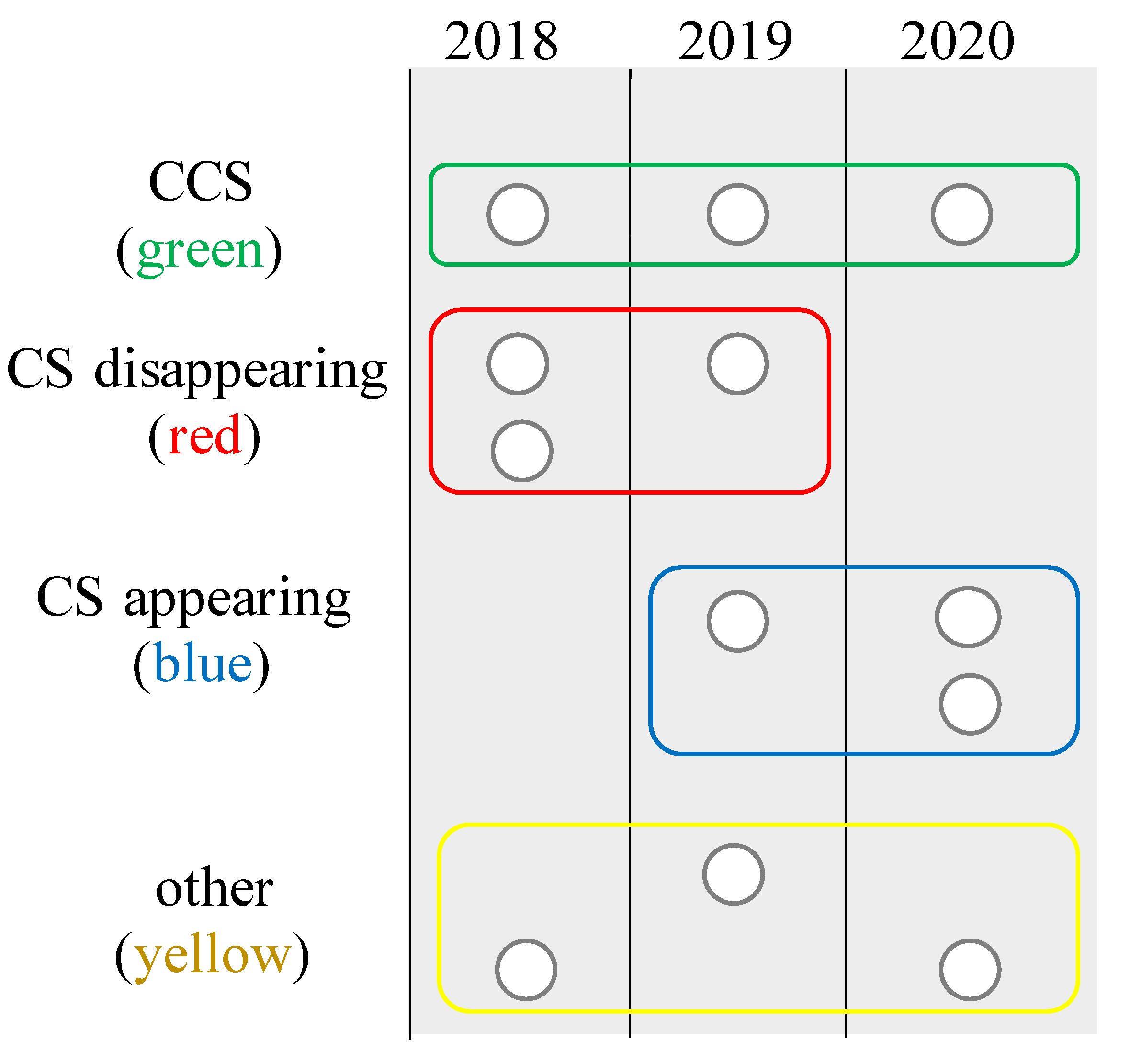
Consequently, we obtained a different number of CSs for each subset. The pixels that show CSs from the first to last subset are referred to as “continuous CS (CCS),” while the pixels that show CSs for only part of subsets are referred to as “TCS” in our approach. To distinguish this approach from the conventional method that has no subset separation, hereafter, the proposed temporal subset SBAS approach is referred to as SUBSET, while the conventional method is referred to as WHOLE.

3.3. Evaluation of SUBSET with a Simulated Environment

The impacts of the subset separation timing and the number of subsets K for the SUBSET approach were investigated with a simulated environment. We simulated a stack of interferometric phase images ( 50 × 50 pixels) with a temporal decorrelation model. The temporal coherence γ tp was computed for both WHOLE and SUBSET. The simulation was conducted by the following procedure:
  • Noise-free raw phase series are first simulated based on an arbitrary deformation phase model ϕ sim = 4 π d sim / λ . We adopt linear subsidence with a yearly trend model by d sim = 100 1092 t + 10 sin 2 π t 365 in millimeters, where t denotes the number of days from the initial date.
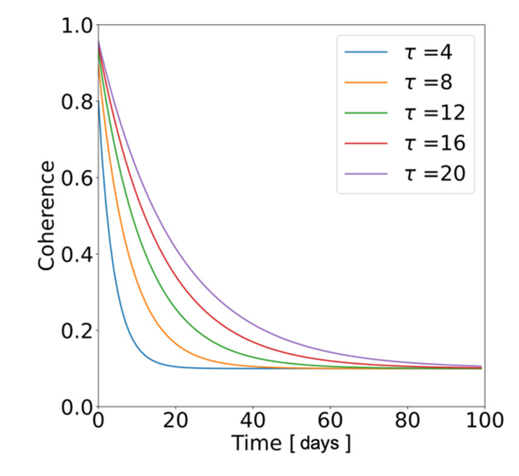
  • Spatial coherence is computed based on the temporal decorrelation model with exponential decay [38],
    γ decorr = 1 γ e t τ + γ ,  
    where γ accounts for the infinite value of coherence and τ is the time for the coherence to drop to 1 / e   of its initial value. Figure 7 shows examples of the temporal decorrelation model for several τ values from 4 to 20 with γ = 0.1 . Note that other decorrelation sources that exist in actual data, such as geometric decorrelation, doppler centroid decorrelation, volume decorrelation, thermal or system noise decorrelation, and processing-induced decorrelation [46], were omitted from this simulation for simplicity.
    Figure 7. Temporal decorrelation model employed in the simulation. τ is varied from 4 to 20 with γ = 0.1 .
    Figure 7. Temporal decorrelation model employed in the simulation. τ is varied from 4 to 20 with γ = 0.1 .
    Remotesensing 14 05825 g007
  • Interferometric phase noises are statistically simulated based on the following probability density function (pdf) [43],
    p d f Δ ϕ = 1 γ decorr 2 L 2 π Γ 2 L 1 Γ L 2 2 2 L 1 × 2 L 1 β 1 β 2 L + 1 2 π 2 + arcsin β + 1 1 β 2 L + 1 2 L 1 r = 0 L 2 Γ L 1 2 Γ L 1 2 r Γ L 1 r Γ L 1 1 + 2 r + 1 β 2 1 β 2 r + 2 ,  
    with β = γ decorr cos Δ ϕ Δ ϕ 0 where Δ ϕ 0 is the expected interferometric phase E Δ ϕ , Γ · is the gamma function, and L denotes the number of looks. We set Δ ϕ 0 and L as 0 and 25, respectively, in this simulation. Phase noises are generated by a normalized cumulative sum of the pdf. Finally, generated interferometric phase noises are added to the noise-free phase generated in step 1.
  • Phase variance σ Δ ϕ i 2 for each interferogram and pixel is calculated by a 5 × 5 moving spatial window on the interferogram images generated in step 3. Spatial coherence is then estimated by the relationship γ sp = 1 / 1 + 2 L σ Δ ϕ i 2 .
  • Raw phase time series are estimated by a WLS solution using the derived phase variances. Finally, the temporal coherence γ tp is computed based on (6). Note that γ tp derived in this simulation was expected to be lower than that in real cases because it does not account for possible phase unwrapping errors and other decorrelation sources.
In total, 267 interferograms ( 50 × 50 pixels) were simulated. Those were formed by 91 simulated raw phase images using the sequential network with three nearest-neighbor connections where the observation time of the raw phase series is the same as that of the Frame 3 data. Under this simulation, we performed three types of analysis, as described below.
First, we investigated the γ tp dependency on the decorrelation models. We varied τ from 4 to 20 days with γ = 0.1   and calculated γ tp for both SUBSET and WHOLE. SUBSET with 
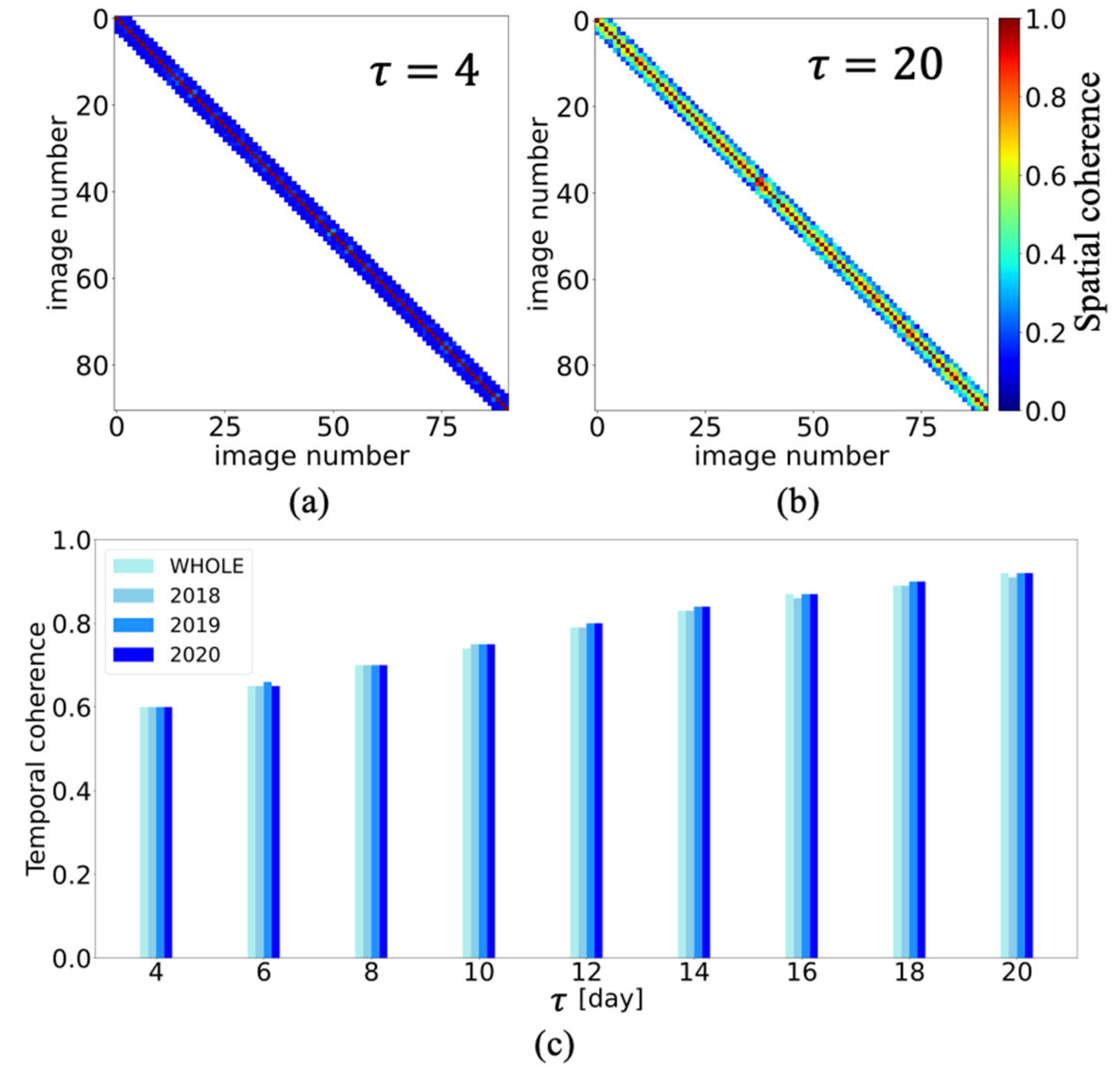
K=3 separated by equal intervals was evaluated in this simulation, that is, data were separated by year. The generated three subsets are 2018, 2019, and 2020, respectively. The spatial coherence matrices of WHOLE for τ = 4 and τ = 20 are shown as examples in Figure 8a,b. Those spatial coherence matrices show higher spatial coherence for higher τ value. A bar plot of the resulting γ tp is shown in Figure 8c. Figure 8c shows an increasing trend of γ tp from 0.6 to 0.92 as τ increases. Figure 8c also reveals similar values for SUBSET (2018, 2019, and 2020) and WHOLE because we applied the same decorrelation model to all the periods. Therefore, it is shown that the data separation done in SUBSET does not alter the γ tp under the uniform decorrelation model.
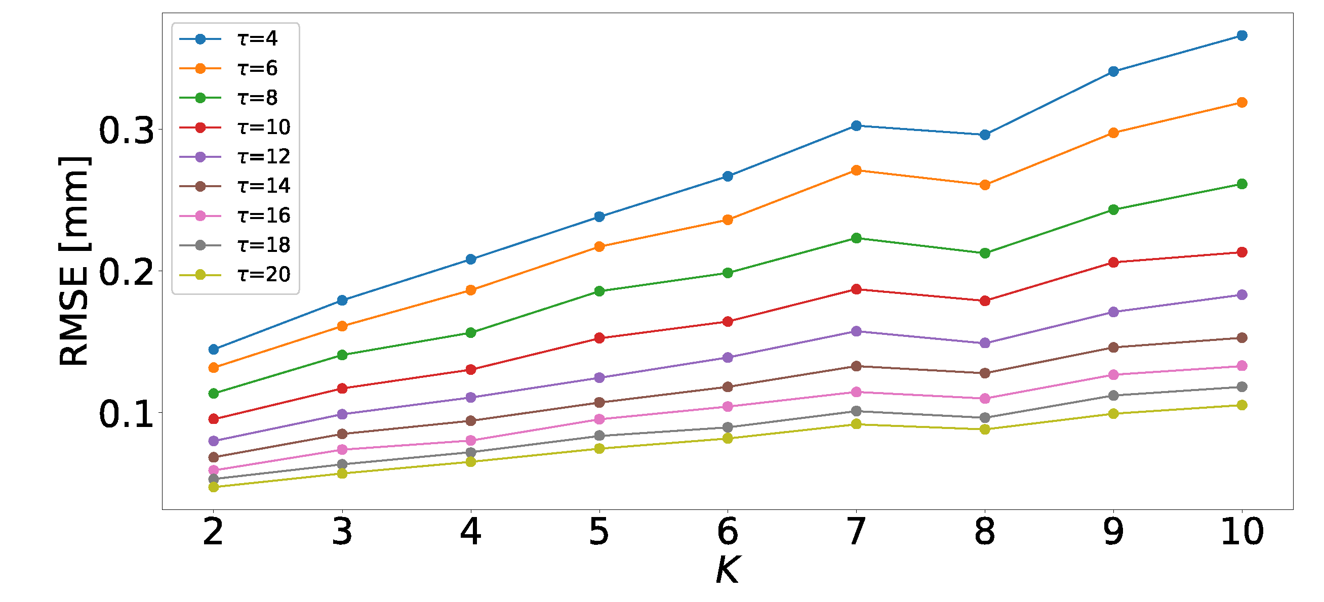
Increasing the number of subsets K is a reasonable strategy for isolating the decorrelated period, and it yields subsets with less decorrelation noise. However, the accuracy of deformation retrieval is expected to be degraded as the number of SLC images in each subset decreases. Thus, we investigated the relationship between the estimated deformation accuracy and the number of subsets K as the second analysis. For this analysis, we varied K from 2 to 10. For SUBSET, the simulated phase series was separated by equal intervals. In this analysis, the τ of the temporal decorrelation model was also varied. We evaluated the estimation accuracy using a root mean square error (RMSE), given by
R M S E = 1 N 1 j = 1 N ϕ ^ j ϕ j sim 2 ,
where ϕ j sim denotes j-th simulated phase value at simulation step 1. The simulation results are summarized in Figure 9 for different τ values. Figure 9 shows an increase in RMSE value as K increases, as well as when τ decreases. In addition, results with lower τ indicate steeper increases in the RMSE with respect to K.
The third analysis considered a non-uniform decorrelation model case, simulating the scatter change within the three-year observation period. For this purpose, we prepared two decorrelation models: (1) vegetation model with τ = 12 and γ = 0.1 and (2) bare surface model with τ = 50 and γ = 0.4 . The decorrelation model was interchanged when scatterers were modified. Vegetation loss was simulated by interchanging from vegetation to bare surface decorrelation models. In this simulation, we tested several decorrelation model transition timings for a variety of situations by testing five timing cases: (1) 1 July 2018, (2) 1 January 2019, (3) 1 July 2019, (4) 1 January 2020, and (5) 1 July 2020. The spatial coherence matrices corresponding to each timing are given in Figure 10a–e, showing distinct patterns of spatial coherence before and after the interchange as the noise level changes. SUBSET with K = 3 separated by equal intervals was evaluated in this simulation. The γ tp values of both methods are shown in Figure 10f. The obtained γ tp reveals different values for SUBSET and WHOLE, with a maximum difference of 0.2. Based on the result in Figure 10f, subsets that avoid the vegetation model always give higher γ tp than that of WHOLE. The amount of decorrelation noise in the subset highly depends on the timing of the scatterer change, meaning that the subset separation timing is considered a key factor for SUBSET.
From the second and third analyses, it is shown that SUBSET enhances the γ tp and RMSE when the optimal subset timing and lower K are appropriately applied.

4. Results

This section provides deformation velocity results by both the SUBSET and WHOLE methods. For SUBSET, we adopted a separation of the equal interval with K = 3, and applied it to the three-year SAR dataset (from January 2018 to January 2021). Therefore, each subset accounts for data of 2018, 2019, and 2020, and a deformation result was obtained for each subset. Under this analysis, we compared the deformation result performance between SUBSET and WHOLE. In addition, a new representation to visualize temporal CS behavior is demonstrated in this section. Interpretations of the results are given in Section 5.

4.1. Results Comparison of the SUBSET and WHOLE Methods

The deformation time series over the seven Sentinel-1A frames in Kalimantan and Sumatra were estimated. The obtained vertical deformation velocity images are shown in Figure 11, where the areas with gray hatched line correspond to the peatland distribution. Only the selected CSs are shown in the velocity images; specifically, pixels with γ tp < 0.65 were masked in our processing. Note that a positive sign of the presented deformation corresponds to the direction from the target to the SAR sensor.
The estimated deformation velocity results show overall subsidence in peatland areas. The larger subsidence of 2019 is found in Figure 11, signifying the effect of severe drought recorded this year due to the positive IOD. Accelerated peat oxidation and peat shrinkage because of a decrease in GWL are considered to be the main reasons for the larger subsidence in 2019.
A number of CSs were used for performance comparison between the SUBSET and the WHOLE. The comparison result for each frame is shown in Figure 12. Note that SUBSET uses the number of CSs in the union of three sets of CSs for 2018, 2019, and 2020 ( C 2018 , C 2019 , and C 2020 ), that is, C = C 2018 C 2019 C 2020 . The comparison results in Figure 12 reveal a higher number of CSs for SUBSET than for WHOLE in all frames. In particular, SUBSET yields more than double the number of CSs for Frames 3, 4, 5, 6, and 7.

4.2. Color Representation

The temporal subset SBAS method can yield a different number of CSs for each subset, as shown in Figure 11. In particular, the areas indicated by dashed white rectangles in Figure 11e,o show significant changes in the CS distribution and density among subsets. The SUBSET approach allows us to characterize this temporal CS behavior. Four classes are considered in the case of SUBSET with K = 3: (1) CS disappearing (TCS), (2) CS appearing (TCS), (3) CCS, and (4) other (CS appears or disappears only in the middle of subsets). Those class types are demonstrated in Figure 13.
To visualize those classes, we assigned red, blue, green, and yellow colors to the four classes: CS disappearing, CS appearing, CCS, and other, respectively. The resulting color representation images for seven Sentinel-1A frames are shown in the first column of Figure 14. The results show that the east parts of Frame 5 (Figure 14g) and Frame 6 (Figure 14j) have blue areas (CS appearing), which might be caused by vegetation clearance due to massive fires. Moreover, large red areas (CS disappearing) are found in the east parts of Frame 4 (Figure 14d) and Frame 5 (Figure 14g), and the northeast part of Frame 7 (Figure 14m). We expect that such red areas suffer from a coherence decrease due to vegetation growth, as we have demonstrated the evolutional coherence decrease over the oil palm plantation area of Frame 4 in Figure 5b. Further discussion on interpreting the results in Figure 14 is given in Section 5.

5. Discussion

The proposed SUBSET method shows a higher number of CSs than that of the WHOLE method for all frames, as shown in Figure 12. When high decorrelation noise is involved during a certain period, subsets that avoid such decorrelations give higher γ tp values than WHOLE according to the third simulation in 
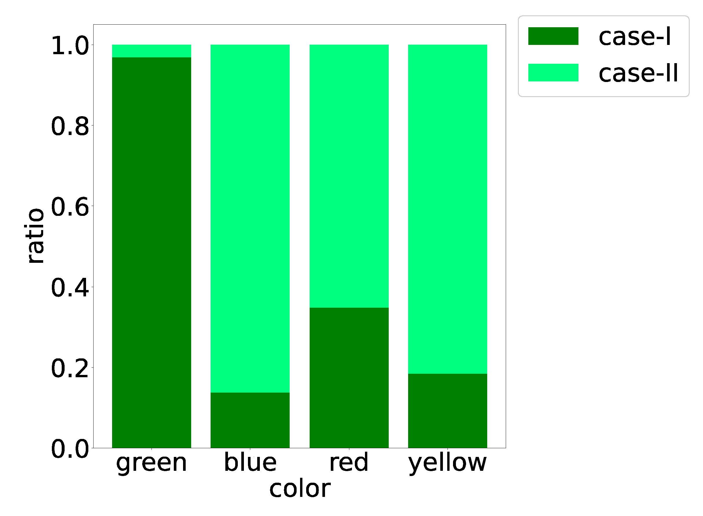
Section 3.3, resulting in a different number of CSs between SUBSET and WHOLE. We herein investigate what kind of CSs are selected by SUBSET but not by WHOLE. For this purpose, two cases of CS are considered: case I, where CSs are selected by SUBSET and WHOLE, and case II, where CSs are selected only by SUBSET. We computed the ratio of two cases for each color, as shown in Figure 15. The result shows that most of the green CCSs are selected by WHOLE. In contrast, red, blue, and yellow reveal a higher ratio in case II, meaning that most of the TCSs are not selected by WHOLE. Therefore, the proposed SUBSET method can enhance the CS density in the areas that show dynamic surface scatterer changes. In particular, significant differences in the CS distribution are found in the regions marked by white dashed rectangles in Figure 11, which correspond to vegetation loss and growth revealed in Figure 4.
We further investigated the causes of the scatterer modification that resulted in TCSs in SUBSET. Scatterer modification within a tropical region is assumed to be predominantly caused by vegetation loss or growth. Investigation of NDVI values gives us a straightforward interpretation of the vegetation condition, namely the amount of vegetation. To check the vegetation change within the observation period, we computed the NDVI for each year in the same way demonstrated in Section 2. The differential images of NDVI computed by N D V I diff = N D V I 2020 N D V I 2018 , where N D V I 2018 and N D V I 2020 represent NDVI values of 2018 and 2020, respectively, are displayed in the second column of Figure 14. Note that the positive and negative values account for vegetation growth and decrease, respectively. The given color maps seem to be related to N D V I diff . For quantitative analysis, Figure 16 shows N D V I diff averaged over the CS corresponding to each color. From the result, the highest positive N D V I diff is found in red, revealing that a disappearing CS is caused by a vegetation increase. In addition, Figure 16 reveals the negative value in blue; hence, the CS appearance is predominantly caused by a vegetation decrease.
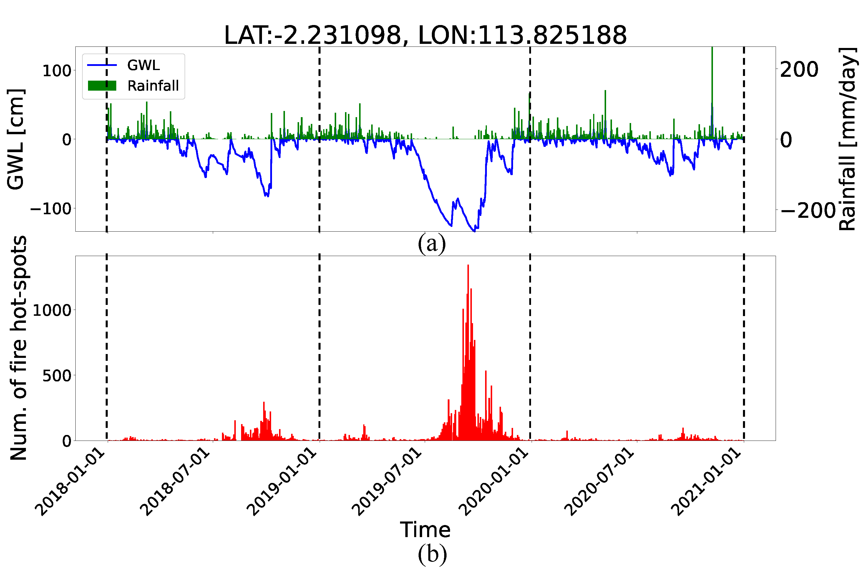
Fires are considered to be one of the reasons for vegetation loss. To investigate the fire effect, we computed the number of fire hotspots by the MODIS Collection 6 active fire/thermal hotspot products for each color and year, as shown in Figure 17. Figure 17 reveals that a significant number of fire hotspots is found in blue pixels, especially for 2019. According to the results in Figure 16 and Figure 17, peat fire is assumed to be the main cause of the CSs appearing.
Furthermore, to demonstrate the relationship between given color maps and land cover classes, we show the 2015 land cover map in the third column of Figure 14. We employed the land cover map produced by Miettinen et al. based on the semi-automated classification of MODIS data supported by various auxiliary data sets [47]. In this study, we updated the oil palm plantation class from Miettinen’s map based on the 2019 oil palm plantation map in [48]. To demonstrate the relationship, the ratio of eight land cover classes for each color is shown in Figure 18. Blue shows the highest ratio of “regrowth/plantation,” indicating that CSs appeared mostly in vegetated areas due to the vegetation clearance and replanting. The result for the blue also indicates a lower ratio of “lowland open” than that of other colors, revealing a lower probability of coherence increase in such open areas. In contrast, the result for red shows the dominance of “lowland open” and “regrowth/plantation” land covers. In addition, red reveals the highest “palm plantation” ratio with respect to other colors. Vegetation growth in such land covers leads to a decrease of spatial coherence with increasing decorrelation noise, resulting in CSs disappearing.

6. Conclusions

The present work investigated an efficient and simple TInSAR approach that accounts for dynamic surface scatterer variation caused by vegetation loss and growth based on the SBAS method. For this, a temporal subset approach was proposed to enhance the number of CSs, leading to a precise investigation of deformation phenomena that occurred on tropical peatland. The scheme of the subset approach was evaluated by InSAR simulation. The simulation investigated the impact of the subset separation timing and the number of subsets in the proposed approach.
We employed Sentinel-1A C-band SAR data to measure deformation with high temporal sampling of tropical peatland in Indonesia and applied the proposed approach. This study adopted the year-based subset strategy for the three-year SAR dataset. Compared with the conventional approach, the proposed approach yielded an improved CS density, especially for areas experiencing vegetation loss or growth. Therefore, the proposed approach gives us a deformation time series that cannot be explored in a conventional way. The SUBSET approach with Sentinel-1 data thus contributes to revealing a more detailed progression of surface deformation occurring in tropical peatland, even short-term deformation (peat oscillation) in response to climatic variations (i.e., changes in GWL). Such monitoring is valuable for evaluating the peat condition and assessing peat restoration.
The CS distribution obtained from three subsets were used to demonstrate a color representation that visually illustrates the CS disappearing and appearing behavior. This distribution was compared with NDVI values and land cover of the study area, revealing a strong relationship between temporal CS behavior and vegetation dynamics.
The length of the time series is expected to continue increasing, as Sentinel-1 has continuously provided images for seven years up to now. The number of TCSs is assumed to increase as the length of the time series increases. Therefore, incorporating the TCS concept in the TInSAR framework is necessary for all kinds of land surface types in the big data era of SAR satellite observations. Future plans include the development of an adaptive solution that efficiently determines the subset timing for the land types in natural areas.

Author Contributions

Conceptualization, Y.I. and W.T.; methodology, Y.I.; software, Y.I.; validation, Y.I.; formal analysis, Y.I. and W.T.; investigation, J.W, A.S., and A.A. (Awaluddin Awaluddin); resources, P.R. and T.A.; data curation, Y.I., W.T., J.W., A.S., A.A. (Awaluddin Awaluddin), and A.A. (Arif Aditiya); writing—original draft preparation, Y.I.; writing—review and editing, Y.I.; visualization, Y.I.; supervision, W.T. and J.T.S.S.; project administration, Y.I.; funding acquisition, Y.I. All authors have read and agreed to the published version of the manuscript.

Funding

This research was funded by the Grand-in-Aid for Research Fellows from the Japan Society for the Promotion of Science, Grant No. 21J00915.

Data Availability Statement

The Sentinel-1 SAR data are publicly available through the Alaska Satellite Facility data portal at https://search.asf.alaska.edu/#/ (accessed on 2 August 2021). MODIS Collection 6 active fire/thermal hotspot products were downloaded from NASA’s Fire Information for Resource Management System at https://firms.modaps.eosdis.nasa.gov/ (accessed on 2 August 2021). The MintPy and InSAR Computing Environment software are open-source and available at https://github.com/insarlab/MintPy (accessed on 2 August 2021) and https://github.com/isce-framework/isce2 (accessed on 2 August 2021), respectively.

Acknowledgments

The authors would like to thank Jukka Miettinen and Soo Chin Liew for providing the 2015 land cover map of Southeast Asia. The authors would also like to thank the Geospatial Information Agency of Indonesia (BIG) for providing GNSS data.

Conflicts of Interest

The authors declare no conflict of interest.

References

  1. Osaki, M.; Kato, T.; Kohyama, T.; Takahashi, H.; Haraguchi, A.; Yabe, K.; Tsuji, N.; Shiodera, S.; Rahajoe, J.S.; Atikah, T.D.; et al. Basic Information about Tropical Peatland Ecosystems BT—Tropical Peatland Eco-Management; Osaki, M., Tsuji, N., Foead, N., Rieley, J., Eds.; Springer Singapore: Singapore, 2021; pp. 3–62. ISBN 9789813346543. [Google Scholar]
  2. Hooijer, A.; Silvius, M.; Woesten, H.; Page, S. PEAT-CO2 Assessment of CO2 Emissions from Drained Peatlands in SE Asia; Delft Hydraulics: Delft, The Netherlands, 2006. [Google Scholar]
  3. Langner, A.; Miettinen, J.; Siegert, F. Land Cover Change 2002–2005 in Borneo and the Role of Fire Derived from MODIS Imagery. Glob. Chang. Biol. 2007, 13, 2329–2340. [Google Scholar] [CrossRef]
  4. Hirano, T.; Kusin, K.; Limin, S.; Osaki, M. Carbon Dioxide Emissions through Oxidative Peat Decomposition on a Burnt Tropical Peatland. Glob. Chang. Biol. 2014, 20, 555–565. [Google Scholar] [CrossRef] [PubMed]
  5. Evans, C.D.; Callaghan, N.; Jaya, A.; Grinham, A.; Sjogersten, S.; Page, S.E.; Harrison, M.E.; Kusin, K.; Kho, L.K.; Ledger, M.; et al. A Novel Low-Cost, High-Resolution Camera System for Measuring Peat Subsidence and Water Table Dynamics. Front. Environ. Sci. 2021, 9, 33. [Google Scholar] [CrossRef]
  6. Howie, S.A.; Hebda, R.J. Bog Surface Oscillation (Mire Breathing): A Useful Measure in Raised Bog Restoration. Hydrol. Process. 2018, 32, 1518–1530. [Google Scholar] [CrossRef]
  7. Osmanoğlu, B.; Sunar, F.; Wdowinski, S.; Cabral-Cano, E. Time Series Analysis of InSAR Data: Methods and Trends. ISPRS J. Photogramm. Remote Sens. 2016, 115, 90–102. [Google Scholar] [CrossRef]
  8. Zhou, Z.; Li, Z.; Waldron, S.; Tanaka, A. InSAR Time Series Analysis of L-Band Data for Understanding Tropical Peatland Degradation and Restoration. Remote Sens. 2019, 11, 2592. [Google Scholar] [CrossRef] [Green Version]
  9. Hoyt, A.M.; Chaussard, E.; Seppalainen, S.S.; Harvey, C.F. Widespread Subsidence and Carbon Emissions across Southeast Asian Peatlands. Nat. Geosci. 2020, 13, 435–440. [Google Scholar] [CrossRef]
  10. Umarhadi, D.A.; Avtar, R.; Widyatmanti, W.; Johnson, B.A.; Yunus, A.P.; Khedher, K.M.; Singh, G. Use of Multifrequency (C-Band and L-Band) SAR Data to Monitor Peat Subsidence Based on Time-Series SBAS InSAR Technique. L. Degrad. Dev. 2021, 32, 4779–4794. [Google Scholar] [CrossRef]
  11. Umarhadi, D.A.; Widyatmanti, W.; Kumar, P.; Yunus, A.P.; Khedher, K.M.; Kharrazi, A.; Avtar, R. Tropical Peat Subsidence Rates Are Related to Decadal LULC Changes: Insights from InSAR Analysis. Sci. Total Environ. 2021, 816, 151561. [Google Scholar] [CrossRef]
  12. Khakim, M.Y.N.; Bama, A.A.; Yustian, I.; Poerwono, P.; Tsuji, T.; Matsuoka, T. Peatland Subsidence and Vegetation Cover Degradation as Impacts of the 2015 El Niño Event Revealed by Sentinel-1A SAR Data. Int. J. Appl. Earth Obs. Geoinf. 2020, 84, 101953. [Google Scholar] [CrossRef]
  13. Marshall, C.; Large, D.J.; Athab, A.; Evers, S.L.; Sowter, A.; Marsh, S.; Sjögersten, S. Monitoring Tropical Peat Related Settlement Using ISBAS InSAR, Kuala Lumpur International Airport (KLIA). Eng. Geol. 2018, 244, 57–65. [Google Scholar] [CrossRef]
  14. Even, M.; Schulz, K. InSAR Deformation Analysis with Distributed Scatterers: A Review Complemented by New Advances. Remote Sens. 2018, 10, 744. [Google Scholar] [CrossRef] [Green Version]
  15. Ferretti, A.; Prati, C.; Rocca, F. Permanent Scatterers in SAR Interferometry. IEEE Trans. Geosci. Remote Sens. 1999, 39, 1528–1530. [Google Scholar] [CrossRef]
  16. Ferretti, A.; Prati, C.; Rocca, F. Nonlinear Subsidence Rate Estimation Using Permanent Scatterers in Differential SAR Interferometry. IEEE Trans. Geosci. Remote Sens. 2000, 38, 2202–2212. [Google Scholar] [CrossRef] [Green Version]
  17. Hooper, A.J. A Multi-Temporal InSAR Method Incorporating Both Persistent Scatterer and Small Baseline Approaches. Geophys. Res. Lett. 2008, 35, 34654. [Google Scholar] [CrossRef] [Green Version]
  18. Ferretti, A.; Fumagalli, A.; Novali, F.; Prati, C.; Rocca, F.; Rucci, A. A New Algorithm for Processing Interferometric Data-Stacks: SqueeSAR. IEEE Trans. Geosci. Remote Sens. 2011, 49, 3460–3470. [Google Scholar] [CrossRef]
  19. Fornaro, G.; Verde, S.; Reale, D.; Pauciullo, A. CAESAR: An Approach Based on Covariance Matrix Decomposition to Improve Multibaseline–Multitemporal Interferometric SAR Processing. IEEE Trans. Geosci. Remote Sens. 2015, 53, 2050–2065. [Google Scholar] [CrossRef]
  20. Ansari, H.; De Zan, F.; Bamler, R. Efficient Phase Estimation for Interferogram Stacks. IEEE Trans. Geosci. Remote Sens. 2018, 56, 4109–4125. [Google Scholar] [CrossRef]
  21. Samiei-Esfahany, S.; Martins, J.E.; van Leijen, F.; Hanssen, R.F. Phase Estimation for Distributed Scatterers in InSAR Stacks Using Integer Least Squares Estimation. IEEE Trans. Geosci. Remote Sens. 2016, 54, 5671–5687. [Google Scholar] [CrossRef] [Green Version]
  22. Berardino, P.; Fornaro, G.; Lanari, R.; Sansosti, E. A New Algorithm for Surface Deformation Monitoring Based on Small Baseline Differential SAR Interferograms. IEEE Trans. Geosci. Remote Sens. 2002, 40, 2375–2383. [Google Scholar] [CrossRef]
  23. Li, S.; Xu, W.; Li, Z. Review of the SBAS InSAR Time-Series Algorithms, Applications, and Challenges. Geod. Geodyn. 2022, 13, 114–126. [Google Scholar] [CrossRef]
  24. Yunjun, Z.; Fattahi, H.; Amelung, F. Small Baseline InSAR Time Series Analysis: Unwrapping Error Correction and Noise Reduction. Comput. Geosci. 2019, 133, 104331. [Google Scholar] [CrossRef] [Green Version]
  25. Hu, F.; Wu, J.; Chang, L.; Hanssen, R.F. Incorporating Temporary Coherent Scatterers in Multi-Temporal InSAR Using Adaptive Temporal Subsets. IEEE Trans. Geosci. Remote Sens. 2019, 57, 7658–7670. [Google Scholar] [CrossRef] [Green Version]
  26. Ferretti, A.; Colesanti, C.; Perissin, D.; Prati, C.; Rocca, F. Evaluating the Effect of the Observation Time on the Distribution of SAR Permanent Scatterers. In Proceedings of the 3rd International Workshop ERS SAR Interferometry (FRINGE), Frascati, Italy, 1–5 December 2003; pp. 1–5. [Google Scholar]
  27. Dogan, O.; Perissin, D. Detection of Multitransition Abrupt Changes in Multitemporal SAR Images. IEEE J. Sel. Top. Appl. Earth Obs. Remote Sens. 2014, 7, 3239–3247. [Google Scholar] [CrossRef]
  28. Brcic, R.; Adam, N. Detecting Changes in Persistent Scatterers. In Proceedings of the 2013 IEEE International Geoscience and Remote Sensing Symposium—IGARSS, Melbourne, Australia, 21–26 July 2013; pp. 117–120. [Google Scholar]
  29. Ansari, H.; Adam, N.; Brcic, R. Amplitude Time Series Analysis in Detection of Persistent and Temporal Coherent Scatterers. In Proceedings of the 2014 IEEE Geoscience and Remote Sensing Symposium, Quebec City, QC, Canada, 3–18 July 2014; pp. 2213–2216. [Google Scholar]
  30. Monti-Guarnieri, A.V.; Brovelli, M.A.; Manzoni, M.; d’Alessandro, M.M.; Molinari, M.E.; Oxoli, D. Coherent Change Detection for Multipass SAR. IEEE Trans. Geosci. Remote Sens. 2018, 56, 6811–6822. [Google Scholar] [CrossRef]
  31. Dommain, R.; Couwenberg, J.; Glaser, P.H.; Joosten, H.; Suryadiputra, I.N.N. Carbon Storage and Release in Indonesian Peatlands since the Last Deglaciation. Quat. Sci. Rev. 2014, 97, 1–32. [Google Scholar] [CrossRef]
  32. Hendon, H.H. Indonesian Rainfall Variability: Impacts of ENSO and Local Air–Sea Interaction. J. Clim. 2003, 16, 1775–1790. [Google Scholar] [CrossRef]
  33. Saji, N.H.; Goswami, B.N.; Vinayachandran, P.N.; Yamagata, T. A Dipole Mode in the Tropical Indian Ocean. Nature 1999, 401, 360–363. [Google Scholar] [CrossRef]
  34. Yamanaka, M.D. Global and Indonesian Climate in 2019. In Toward the Regeneration of Tropical Peatmland Societies; Newsletter; Tropical Peatland Society Project at Research Institute for Humanity and Nature: Kyoto, Japan, 2020; Volume 8, pp. 6–7. [Google Scholar]
  35. Takeuchi, W.; Hirano, T.; Roswintiarti, O. Estimation Model of Ground Water Table at Peatland in Central Kalimantan, Indonesia. In Tropical Peatland Ecosystems; Springer: Tokyo, Japan, 2016; pp. 445–453. [Google Scholar] [CrossRef]
  36. Park, H.; Takeuchi, W.; Ichii, K. Satellite-Based Estimation of Carbon Dioxide Budget in Tropical Peatland Ecosystems. Remote Sens. 2020, 12, 250. [Google Scholar] [CrossRef]
  37. Villarroya-Carpio, A.; Lopez-Sanchez, J.M.; Engdahl, M.E. Sentinel-1 Interferometric Coherence as a Vegetation Index for Agriculture. Remote Sens. Environ. 2022, 280, 113208. [Google Scholar] [CrossRef]
  38. Morishita, Y.; Hanssen, R.F. Temporal Decorrelation in L-, C-, and X-Band Satellite Radar Interferometry for Pasture on Drained Peat Soils. IEEE Trans. Geosci. Remote Sens. 2015, 53, 1096–1104. [Google Scholar] [CrossRef]
  39. De Zan, F.; Guarnieri, A.M. TOPSAR: Terrain Observation by Progressive Scans. IEEE Trans. Geosci. Remote Sens. 2006, 44, 2352–2360. [Google Scholar] [CrossRef]
  40. Fattahi, H.; Agram, P.; Simons, M. A Network-Based Enhanced Spectral Diversity Approach for TOPS Time-Series Analysis. IEEE Trans. Geosci. Remote Sens. 2017, 55, 777–786. [Google Scholar] [CrossRef] [Green Version]
  41. Chen, C.W.; Zebker, H.A. Phase Unwrapping for Large SAR Interferograms: Statistical Segmentation and Generalized Network Models. IEEE Trans. Geosci. Remote Sens. 2002, 40, 1709–1719. [Google Scholar] [CrossRef] [Green Version]
  42. Aditiya, A.; Efendi, J.; Arief Syafii, M. InaCORS: Infrastructure of GNSS CORS in Indonesia. In Proceedings of the FIG Congress 2014, Kuala Lumpur, Malaysia, 16–21 June 2014. [Google Scholar]
  43. Tough, J.A.; Blacknell, D.; Quegan, S. A Statistical Description of Polarimetric and Interferometric Synthetic Aperture Radar Data. Proc. R. Soc. London. Ser. A Math. Phys. Sci. 1995, 449, 567–589. [Google Scholar] [CrossRef]
  44. Jolivet, R.; Grandin, R.; Lasserre, C.; Doin, M.P.; Peltzer, G. Systematic InSAR Tropospheric Phase Delay Corrections from Global Meteorological Reanalysis Data. Geophys. Res. Lett. 2011, 38. [Google Scholar] [CrossRef] [Green Version]
  45. Fattahi, H.; Amelung, F. DEM Error Correction in InSAR Time Series. IEEE Trans. Geosci. Remote Sens. 2013, 51, 4249–4259. [Google Scholar] [CrossRef]
  46. Hanssen, R.F. Radar Interferometry: Data Interpretation and Error Analysis; Kluwer: Dordrecht, The Netherlands, 2001; ISBN 9780792369455. [Google Scholar]
  47. Miettinen, J.; Shi, C.; Liew, S.C. 2015 Land Cover Map of Southeast Asia at 250 m Spatial Resolution. Remote Sens. Lett. 2016, 7, 701–710. [Google Scholar] [CrossRef]
  48. Descals, A.; Wich, S.; Meijaard, E.; Gaveau, D.L.A.; Peedell, S.; Szantoi, Z. High-Resolution Global Map of Smallholder and Industrial Closed-Canopy Oil Palm Plantations. Earth Syst. Sci. Data 2021, 13, 1211–1231. [Google Scholar] [CrossRef]
Figure 1. Study area over Kalimantan and Sumatra in Indonesia. Black rectangles indicate the Sentinel-1A frames processed in this study. The reddish-brown areas represent peatlands.
Remotesensing 14 05825 g001
Figure 2. Landsat 8 true color images of each frame (RGB: bands 4, 3, and 2). (a) Frames 1, 2, and 3. (b) Frame 4. (c) Frame 5. (d) Frames 6 and 7.
Remotesensing 14 05825 g002
Figure 3. Time series of rainfall, GWL, and the number of fire hotspots from January 2018 to December 2020. (a) Rainfall and estimated GWL at a single point (latitude/longitude: −2.23/113.825) near Palangka Raya city within Frame 1. (b) Number of daily fire hotspots over the study area during the investigated period.
Remotesensing 14 05825 g003
Figure 4. Yearly NDVI images for 2018, 2019, and 2020 in the study areas. (a) Jambi in 2018. (b) Jambi in 2019. (c) Jambi in 2020. (d) West Kalimantan in 2018. (e) West Kalimantan in 2019. (f) West Kalimantan in 2020.
Remotesensing 14 05825 g004
Figure 5. Time series of average spatial coherence. (a) Spatial coherence averaged over the red polygons in Figure 4a–c. (b) Spatial coherence averaged over the red polygons in Figure 4d–f.
Remotesensing 14 05825 g005
Figure 6. Process flow in the SUBSET method. In this example, the three-year time series SAR dataset is separated into three single-year datasets (2018, 2019, and 2020). The interferograms are formed by SLC images corresponding to each subset through a sequential network. This figure uses the perpendicular baseline and observation date of Frame 3 as an example.
Remotesensing 14 05825 g006
Figure 8. Simulation results of varying τ from 4 to 20 days with γ = 0.1 for SUBSET and WHOLE. (a) Spatial coherence matrix with τ = 4 . (b) Spatial coherence matrix with τ = 20 . (c) Temporal coherence bar plot for SUBSET and WHOLE.
Remotesensing 14 05825 g008
Figure 9. RMSE variation with respect to K for different τ values.
Remotesensing 14 05825 g009
Figure 10. Simulation results of two decorrelation models. (a)–(e) Spatial coherence matrix for each model transition timing. (a) 1 July 2018. (b) 1 January 2019. (c) 1 July 2019. (d) 1 January 2020. (e) 1 July 2020. (f) Temporal coherence bar plot for both SUBSET and WHOLE.
Remotesensing 14 05825 g010
Figure 11. Vertical deformation velocity images for seven Sentinel-1A frames derived by SUBSET and WHOLE. (a) SUBSET 2018 result for Frames 1,2, and 3. (b) SUBSET 2019 result for Frames 1,2, and 3. (c) SUBSET 2020 result for Frames 1,2, and 3. (d) WHOLE result for Frames 1,2, and 3. (e) SUBSET 2018 result for Frame 4. (f) SUBSET 2019 result for Frame 4. (g) SUBSET 2020 result for Frame 4. (h) WHOLE result for Frame 4. (i) SUBSET 2018 result for Frame 5. (j) SUBSET 2019 result for Frame 5. (k) SUBSET 2020 result for Frame 5. (l) WHOLE result for Frame 5. (m) SUBSET 2018 result for Frame 6. (n) SUBSET 2019 result for Frame 6. (o) SUBSET 2020 result for Frame 6. (p) WHOLE result for Frame 6. (q) SUBSET 2018 result for Frame 7. (r) SUBSET 2019 result for Frame 7. (s) SUBSET 2020 result for Frame 7. (t) WHOLE result for Frame 7.
Remotesensing 14 05825 g011
Figure 12. Number of CSs achieved by SUBSET and WHOLE for the seven investigated frames.
Remotesensing 14 05825 g012
Figure 13. Schematic demonstration of class types in color representation. White circles indicate the existence of CSs.
Remotesensing 14 05825 g013
Figure 14. Results of processing and Land cover maps. (a) Color map for Frames 1, 2, and 3. (b) N D V I diff for Frames 1, 2, and 3. (c) Land cover map for Frames 1, 2, and 3. (d) Color map for Frame 4. (e) N D V I diff for Frame 4. (f) Land cover map for Frame 4. (g) Color map for Frame 5. (h) N D V I diff for Frame 5. (i) Land cover map for Frame 5. (j) Color map for Frame 6. (k) N D V I diff for Frame 6. (l) Land cover map for Frame 6. (m) Color map for Frame 7. (n) N D V I diff for Frame 7. (o) Land cover map for Frame 7.
Remotesensing 14 05825 g014
Figure 15. Ratio of case I to case II for each color.
Remotesensing 14 05825 g015
Figure 16. Average N D V I diff values over the CSs corresponding to each color.
Remotesensing 14 05825 g016
Figure 17. Total number of fire hotspots summed over the pixels corresponding to each color.
Remotesensing 14 05825 g017
Figure 18. Ratio of eight land cover classes for each color.
Remotesensing 14 05825 g018
Publisher’s Note: MDPI stays neutral with regard to jurisdictional claims in published maps and institutional affiliations.

