
Noise-Robust ISAR Translational Motion Compensation via HLPT-GSCFT

Abstract
:1. Introduction
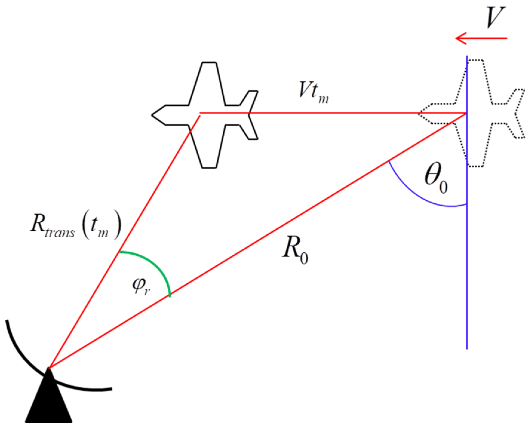
2. Signal Model
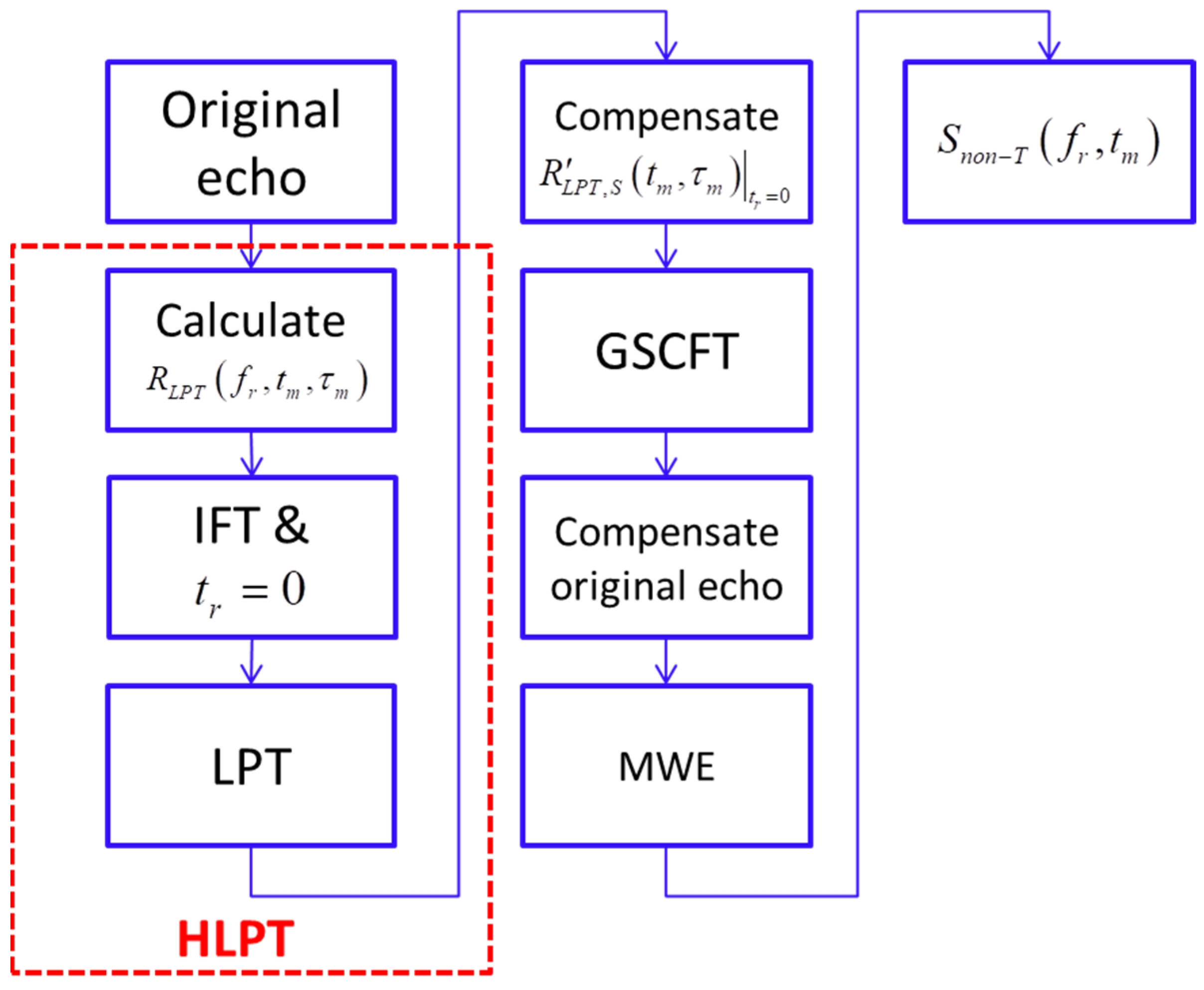
3. Translational Parameter Estimation Based on HLPT-GSCFT
4. Translational Motion Compensation
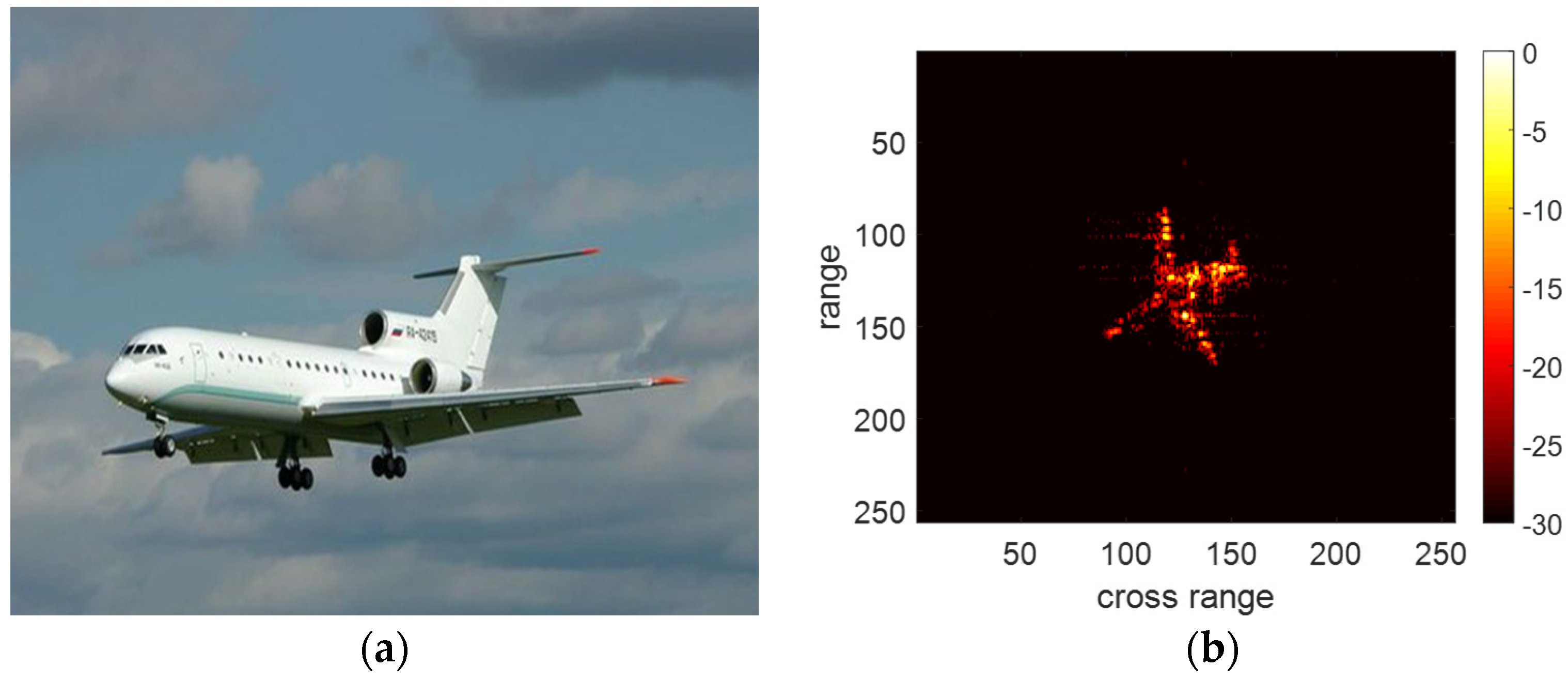
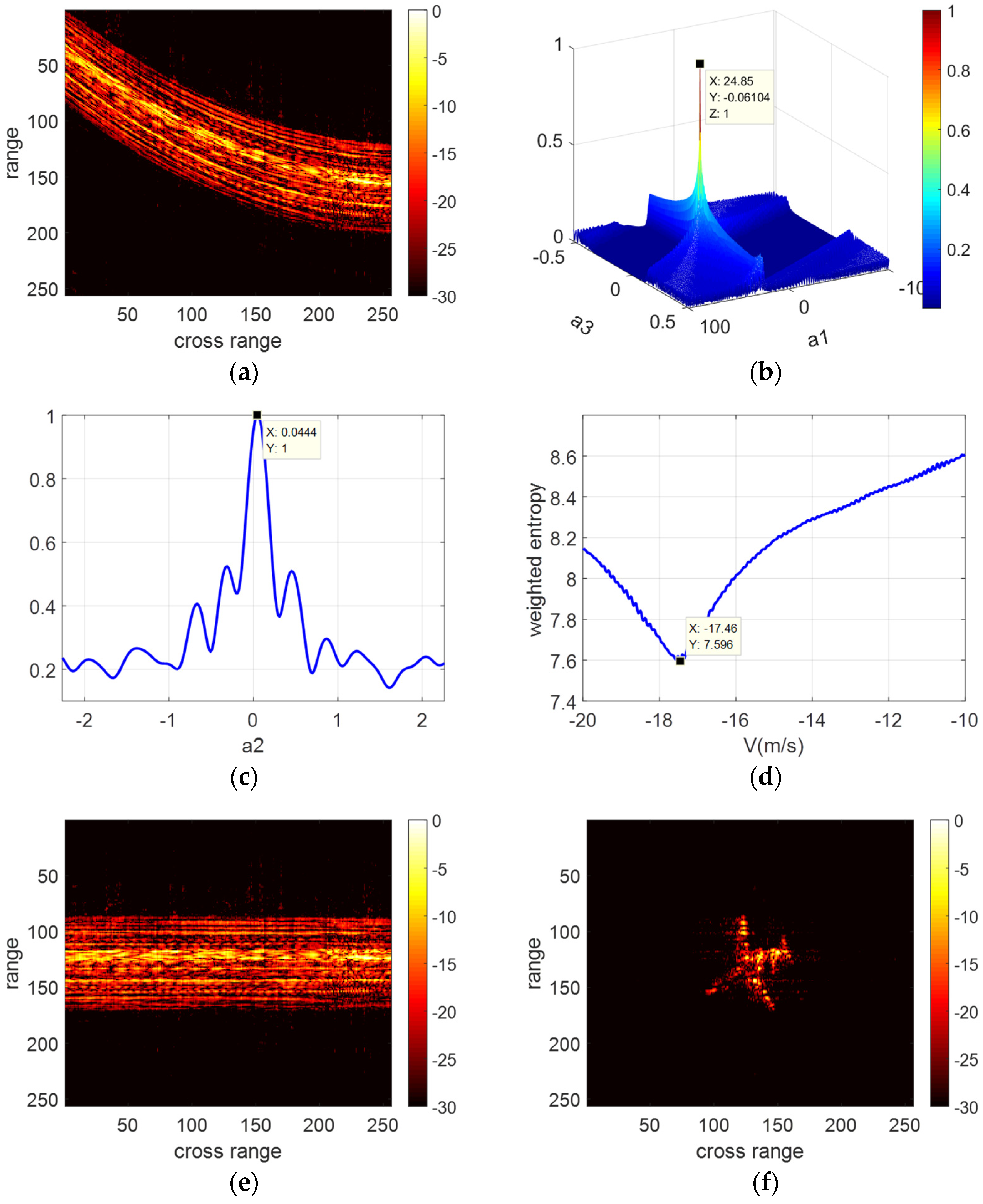
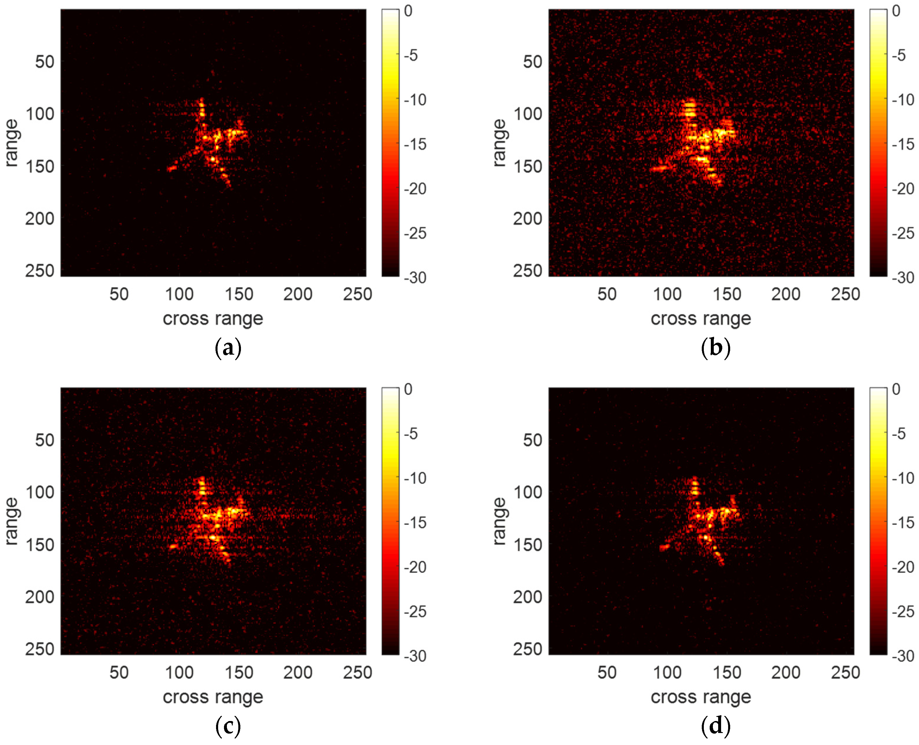
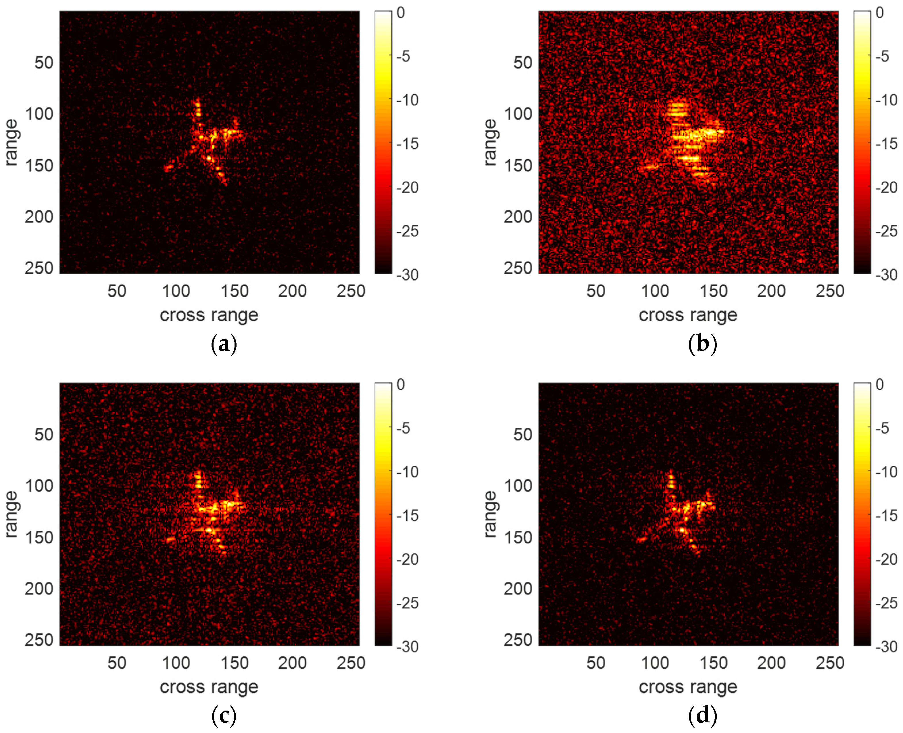
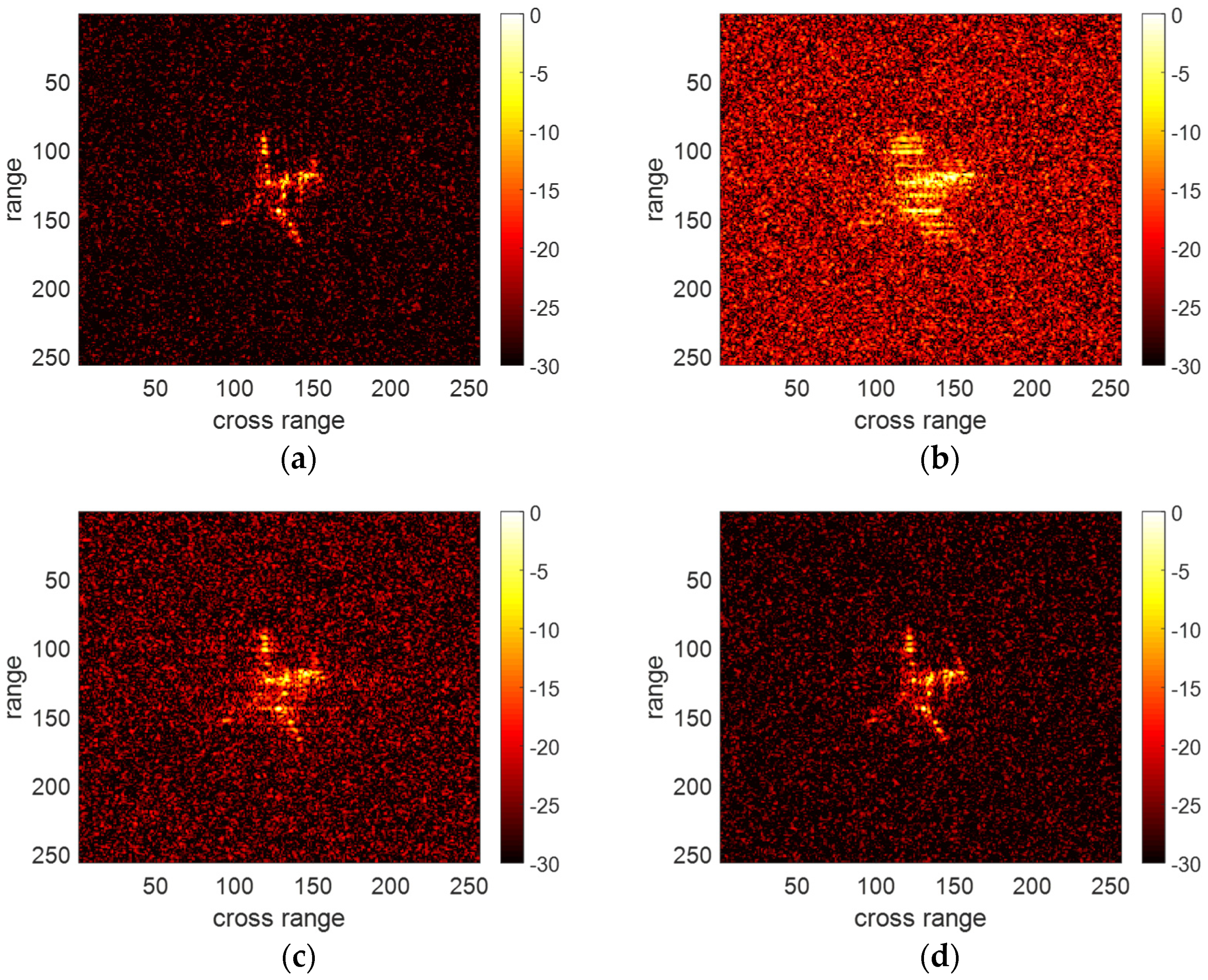
5. Experiment of Yak-42 Measured Dataset
6. Conclusions
Author Contributions
Funding
Data Availability Statement
Acknowledgments
Conflicts of Interest
References
- Chen, C.C.; Andrews, H.C. Target-motion-induced radar imaging. IEEE Trans. Aerosp. Electron. Syst. 1980, 16, 2–14. [Google Scholar] [CrossRef]
- Zhu, D.; Wang, L.; Yu, Y. Robust ISAR range alignment ia minimizing the entropy of the average range profile. IEEE Geosci. Remote Sens. Lett. 2009, 6, 204–208. [Google Scholar]
- Sauer, T.; Schroth, A. Robust range alignment algorithm via Hough transform in an ISAR imaging system. IEEE Trans. Aerosp. Electron. Syst. 1995, 31, 1173–1177. [Google Scholar] [CrossRef]
- Lee, S.-H.; Bae, J.-H.; Kang, M.-S.; Kim, C.-H.; Kim, K.-T. ISAR autofocus by minimizing entropy of eigenimages. In Proceedings of the 2016 IEEE Radar Conference (RadarConf), Philadelphia, PA, USA, 2–6 May 2016. [Google Scholar]
- Xu, J.; Cai, J.; Sun, Y.; Xia, X.-G.; Farina, A.; Long, T. Efficient ISAR Phase Autofocus Based on Eigenvalue Decomposition. IEEE Geosci. Remote Sens. Lett. 2017, 14, 2195–2199. [Google Scholar] [CrossRef]
- Cao, P.; Xing, M.; Sun, G.; Li, Y.; Bao, Z. Minimum Entropy via Subspace for ISAR Autofocus. IEEE Geosci. Remote Sens. Lett. 2009, 7, 205–209. [Google Scholar] [CrossRef]
- Cai, J.-J.; Xu, J.; Wang, G.; Xia, X.-G.; Long, T.; Bian, M.-M. An effective ISAR autofocus algorithm based on single eigenvector. In Proceedings of the 2016 CIE International Conference on Radar (RADAR), Guangzhou, China, 10–13 October 2016; pp. 1–5. [Google Scholar] [CrossRef]
- Ye, W.; Yeo, T.S.; Bao, Z. Weighted least-squares estimation of phase errors for SAR/ISAR autofocus. IEEE Trans. Geosci. Remote Sens. 1999, 37, 2487–2494. [Google Scholar] [CrossRef] [Green Version]
- Wahl, D.; Eichel, P.; Ghiglia, D.; Jakowatz, C. Phase gradient autofocus-a robust tool for high resolution SAR phase correction. IEEE Trans. Aerosp. Electron. Syst. 1994, 30, 827–835. [Google Scholar] [CrossRef] [Green Version]
- Chan, H.; Yeo, T.S. Comments on “Non-iterative quality phase-gradient autofocus (QPGA) algorithm for spotlight SAR imagery”. IEEE Trans. Geosci. Remote Sens. 2002, 40, 2517. [Google Scholar] [CrossRef]
- Cai, J.; Martorella, M.; Chang, S.; Liu, Q.; Ding, Z.; Long, T. Efficient Nonparametric ISAR Autofocus Algorithm Based on Contrast Maximization and Newton’s Method. IEEE Sens. J. 2020, 21, 4474–4487. [Google Scholar] [CrossRef]
- Chen, J.; Xing, M.; Yu, H.; Liang, B.; Peng, J.; Sun, G.-C. Motion Compensation/Autofocus in Airborne Synthetic Aperture Radar: A Review. IEEE Geosci. Remote Sens. Mag. 2021, 10, 185–206. [Google Scholar] [CrossRef]
- Marston, T.M.; Plotnick, D.S. Semiparametric Statistical Stripmap Synthetic Aperture Autofocusing. IEEE Trans. Geosci. Remote Sens. 2014, 53, 2086–2095. [Google Scholar] [CrossRef]
- Chen, J.; Zhang, J.; Jin, Y.; Yu, H.; Liang, B.; Yang, D.-G. Real-Time Processing of Spaceborne SAR Data With Nonlinear Trajectory Based on Variable PRF. IEEE Trans. Geosci. Remote Sens. 2021, 60, 1–12. [Google Scholar] [CrossRef]
- Li, X.; Kong, L.; Cui, G.; Yi, W.; Yang, Y. ISAR imaging of maneuvering target with complex motions based on ACCF–LVD. Digit. Signal Process. 2015, 46, 191–200. [Google Scholar] [CrossRef]
- Yuan, Y.; Luo, Y.; Kang, L.; Ni, J.; Zhang, Q. Range Alignment in ISAR Imaging Based on Deep Recurrent Neural Network. IEEE Geosci. Remote Sens. Lett. 2022, 19, 1–5. [Google Scholar] [CrossRef]
- Li, X.; Bai, X.; Zhou, F. High-Resolution ISAR Imaging and Autofocusing via 2D-ADMM-Net. Remote Sens. 2021, 13, 2326. [Google Scholar] [CrossRef]
- Wei, S.; Liang, J.; Wang, M.; Shi, J.; Zhang, X.; Ran, J. AF-AMPNet: A Deep Learning Approach for Sparse Aperture ISAR Imaging and Autofocusing. IEEE Trans. Geosci. Remote Sens. 2021, 60, 1–14. [Google Scholar] [CrossRef]
- Gao, Y.; Xing, M.; Li, Y.; Sun, W.; Zhang, Z. Joint Translational Motion Compensation Method for ISAR Imagery Under Low SNR Condition Using Dynamic Image Sharpness Metric Optimization. IEEE Trans. Geosci. Remote Sens. 2021, 60, 1–15. [Google Scholar] [CrossRef]
- Shao, S.; Zhang, L.; Liu, H.; Zhou, Y. Accelerated translational motion compensation with contrast maximization optimization algorithm for inverse synthetic aperture radar imaging. IET Radar Sonar Navig. 2018, 13, 316–325. [Google Scholar] [CrossRef]
- Fu, J.; Xing, M.; Amin, M.; Sun, G. ISAR Translational Motion Compensation with Simultaneous Range Alignment and Phase Adjustment in Low SNR Environments. In Proceedings of the 2021 IEEE Radar Conference (RadarConf21), Atlanta, GA, USA, 7–14 May 2021; pp. 1–6. [Google Scholar] [CrossRef]
- Zhang, L.; Sheng, J.-L.; Duan, J.; Xing, M.-D.; Qiao, Z.-J.; Bao, Z. Translational motion compensation for ISAR imaging under low SNR by minimum entropy. EURASIP J. Adv. Signal Process. 2013, 2013, 33. [Google Scholar] [CrossRef]
- Ustun, D.; Toktas, A. Translational Motion Compensation for ISAR Images Through a Multicriteria Decision Using Surrogate-Based Optimization. IEEE Trans. Geosci. Remote Sens. 2020, 58, 4365–4374. [Google Scholar] [CrossRef]
- Liu, L.; Zhou, F.; Tao, M.; Sun, P.; Zhang, Z. Adaptive Translational Motion Compensation Method for ISAR Imaging Under Low SNR Based on Particle Swarm Optimization. IEEE J. Sel. Top. Appl. Earth Obs. Remote Sens. 2015, 8, 5146–5157. [Google Scholar] [CrossRef]
- Peng, S.B.; Xu, J.; Peng, Y.N. Parametric inverse synthetic aperture radar manoeuvring target motion compensation based on particle swarm optimizer. IET Radar Sonar Navig. 2011, 5, 305–314. [Google Scholar] [CrossRef]
- Li, D.; Zhan, M.; Liu, H.; Liao, Y.; Liao, G. A Robust Translational Motion Compensation Method for ISAR Imaging Based on Keystone Transform and Fractional Fourier Transform Under Low SNR Environment. IEEE Trans. Aerosp. Electron. Syst. 2017, 53, 2140–2156. [Google Scholar] [CrossRef]
- Zhuo, Z.; Du, L.; Lu, X.; Ren, K.; Li, L. Ambiguity Function based High-Order Translational Motion Compensation. IEEE Trans. Aerosp. Electron. Syst. 2022, 1–8, early access. [Google Scholar] [CrossRef]
- Xing, M.; Wu, R.; Lan, J.; Bao, Z. Migration Through Resolution Cell Compensation in ISAR Imaging. IEEE Geosci. Remote Sens. Lett. 2004, 1, 141–144. [Google Scholar] [CrossRef]
- Ljubiša, S. Local polynomial Wigner distribution. Signal Process. 1997, 59, 123–128. [Google Scholar]
- Wang, Y.; Kang, J.; Jiang, Y. ISAR Imaging of Maneuvering Target Based on the Local Polynomial Wigner Distribution and Integrated High-Order Ambiguity Function for Cubic Phase Signal Model. IEEE J. Sel. Top. Appl. Earth Obs. Remote Sens. 2014, 7, 2971–2991. [Google Scholar] [CrossRef]
- Liu, F.; Feng, C.; Huang, D.; Guo, X. Fast ISAR imaging method for complex manoeuvring target based on local polynomial transform-fast chirp Fourier transform. IET Radar Sonar Navig. 2021, 15, 666–676. [Google Scholar] [CrossRef]
- Lv, Q.; Su, T.; He, X. An ISAR Imaging Algorithm for Nonuniformly Rotating Targets With Low SNR Based on Modified Bilinear Parameter Estimation of Cubic Phase Signal. IEEE Trans. Aerosp. Electron. Syst. 2018, 54, 3108–3124. [Google Scholar] [CrossRef]
- Zheng, J.; Su, T.; Zhu, W.; Zhang, L.; Liu, Z.; Liu, Q.H. ISAR Imaging of Nonuniformly Rotating Target Based on a Fast Parameter Estimation Algorithm of Cubic Phase Signal. IEEE Trans. Geosci. Remote Sens. 2015, 53, 4727–4740. [Google Scholar] [CrossRef]


| Ideal Result | PSO | PD-KT-FrFT | Proposed Method | |
|---|---|---|---|---|
| SNR = −0 dB | 8.2354 | 8.4554 | 8.3455 | 8.2651 |
| SNR = −3 dB | 9.5212 | 9.8930 | 9.6251 | 9.5321 |
| SNR = −6 dB | 10.4501 | 10.6651 | 10.5021 | 10.4589 |
| v | a1 | a2 | a3 | |
|---|---|---|---|---|
| SNR = −9 dB | −17.43 | 24.85 | 0.0444 | −0.061 |
| SNR = −10 dB | −17.48 | 24.85 | 0.0444 | −0.061 |
| SNR = −11 dB | −17.46 | 25.13 | 0.0421 | −0.064 |
| SNR = −12 dB | −17.55 | 25.72 | 0.0457 | −0.057 |
Publisher’s Note: MDPI stays neutral with regard to jurisdictional claims in published maps and institutional affiliations. |
© 2022 by the authors. Licensee MDPI, Basel, Switzerland. This article is an open access article distributed under the terms and conditions of the Creative Commons Attribution (CC BY) license (https://creativecommons.org/licenses/by/4.0/).
Share and Cite
Liu, F.; Huang, D.; Guo, X.; Feng, C. Noise-Robust ISAR Translational Motion Compensation via HLPT-GSCFT. Remote Sens. 2022, 14, 6201. https://doi.org/10.3390/rs14246201
Liu F, Huang D, Guo X, Feng C. Noise-Robust ISAR Translational Motion Compensation via HLPT-GSCFT. Remote Sensing. 2022; 14(24):6201. https://doi.org/10.3390/rs14246201
Chicago/Turabian StyleLiu, Fengkai, Darong Huang, Xinrong Guo, and Cunqian Feng. 2022. "Noise-Robust ISAR Translational Motion Compensation via HLPT-GSCFT" Remote Sensing 14, no. 24: 6201. https://doi.org/10.3390/rs14246201