Article

Focus Improvement of Spaceborne-Missile Bistatic SAR Data Using the Modified NLCS Algorithm Based on the Method of Series Reversion

China Academy of Space Technology (Xi’an), Xi’an 710100, China
*
Author to whom correspondence should be addressed.
Remote Sens. 2022, 14(22), 5770; https://doi.org/10.3390/rs14225770
Submission received: 7 September 2022 / Revised: 23 October 2022 / Accepted: 11 November 2022 / Published: 15 November 2022

Abstract

:
The speed and direction of a missile shifts sharply in the dive phase, making the azimuth frequency modulation (FM) rate change with the azimuthal position, leading to azimuth ambiguities and image distortion. To solve this problem, a modified nonlinear chirp scaling (NLCS) algorithm was adopted to compensate for the azimuth FM rate. First, the geometric configuration and echo signal model of the spaceborne missile bistatic synthetic aperture radar (SAR) were built, and then the Doppler frequency correction was performed, and the 2-D spectrum of the signal was derived by the method of series reversion. Next, range migration correction and range compression were finished in the 2-D frequency domain. Following this, a modified NLCS algorithm was proposed to solve the space variance of Doppler phase problem. After compensating for the azimuth FM rate, the azimuth compression focusing was completed and the imaging result was obtained. Finally, by comparing the calculation amount, imaging effect, and performance index with the traditional NLCS algorithm, it can be concluded that the algorithm reduced the calculation amount by 1.0128 × 10⁸ floating point operations per second (FLOPs) compared with the traditional NLCS algorithm, and the azimuth focusing effect of the edge point was greatly improved. Its resolution, peak sidelobe ratio (PSLR), and integrated sidelobe ratio (ISLR) were improved by 0.87 m, 3.32 dB, and 1.79 dB, respectively, which proved the effectiveness and feasibility of this method.

1. Introduction

The synthetic aperture radar (SAR) can penetrate through all weather conditions and can operate all day long [1,2]. It has been widely used in combat and geological surveys [3,4]. Compared with the traditional monostatic SAR, the new bistatic SAR has the advantages of strong concealment, rich information acquisition, and forward-looking imaging [5]. As the transmitting source, the satellite operates at a certain orbital altitude, with strong anti-strike capability and wide beam coverage [6]. As the receiver, the missile has the advantage of high resolution [7]. The new system of spaceborne missile bistatic SAR can combine the advantages of spaceborne SAR and missile-borne SAR. It can combine the large-scale coverage and high security of spaceborne SAR with the high resolution and high mobility of missile-borne SAR, effectively obtaining scene targets including background, improving the ability to strike targets, and realizing the integration of observation and attack [8,9,10].
Although there are many advantages in the special geometry configuration, it also brings about two challenges in applying the algorithm to processing the echo signal data. First, it is difficult to obtain an accurate expression of the 2-D spectrum for spaceborne missile bistatic SAR, which is the basis of the imaging algorithm. In a bistatic system, the range history is the sum of two hyperbolic range equations, and therefore there is a double square root term in the range history [11], which makes it difficult to solve the 2-D spectrum analytically by directly applying the stationary phase principle [12,13,14,15]. The derivations about the spectrum of the bistatic SAR were completed in [16]. However, these derivations only apply to some special geometric configurations (azimuth-invariant or parallel) that do not directly obtain the analytical solution of the bistatic stationary phase leading to a significant decrease in accuracy. For the flexible spaceborne missile bistatic system, these approaches in [16] cannot be applied to handle it. To solve the accuracy issue, the Legendre expansion [17] and orthogonal expansion [18] methods have been preliminarily studied, but solving a higher-order 2-D spectrum is challenging. The 2-D spectrum was derived in [19] using the Lagrange inversion theorem (LIT). The bistatic stationary phase can be derived while maintaining the double square root of the slant range history. Furthermore, its accuracy is solely determined by the number of analytical solutions retained in the stationary phase. In this paper, we derived the 2-D spectrum of spaceborne missile bistatic SAR by using the method of series reversion [20]. The idea is to apply Taylor expansion to the slant range history, then determine the analytical solution of the stationary phase point by series reversion after removing the linear range cell migration and the linear phase term. The precision of this spectrum is controlled by the two slant range expansions as well as the series reversion.
The second challenge comes from the space variance of the Doppler phase. The modified Omega-K, chirp scaling algorithm, and range-Doppler algorithms reported in [16,21,22,23] are the forward-looking imaging algorithms that are suited for airborne and spaceborne bistatic SAR, but they are not suitable for missile-borne bistatic SAR. Back-projection algorithms are capable of handling general bistatic configurations with topographic dependences and flexible moving platforms [24,25,26,27], but the efficiency of the algorithm is low. A nonlinear chirp scaling algorithm that is more effective for handling data with the bistatic geometry where the transmitter or receiver is stationary has been presented [28,29]. In these papers, the azimuth focusing depth is limited as only the symmetrical azimuth FM rates and the parabolic are considered. Moreover, [30] considers the nonlinear component of azimuth FM rate, but only monostatic squinted missile-borne SAR data can be processed by this algorithm. In [31], a frequency-domain algorithm is proposed for curvilinear flight SAR, which compensates the spatial variation of the Doppler frequency modulation term. However, the residual azimuth spatial variation leads to an affect imaging focus in the azimuth direction for large scenes.
On the basis of the previous research, a modified NLCS algorithm was used to process the data of spaceborne missile bistatic SAR. The algorithm can be divided into the following steps. First, the echo signal and the geometric configuration of spaceborne missile bistatic SAR were established. Then, the Doppler frequency correction operation was conducted in range frequency and the azimuth time domain. Second, the 2-D spectrum of the spaceborne missile bistatic SAR echo signal was successfully derived by the method of series reversion. Following this, the range migration correction and range compression were completed in the 2-D frequency domain, and the imaging position in the range was determined. Finally, a modified NLCS algorithm was applied to compensate for the azimuth FM rate, eliminating the distortion of the image in azimuth, and a great imaging result was presented in the simulation.
The rest of the paper is organized as follows. Section 2 establishes the geometry of the spaceborne missile bistatic SAR and builds the echo signal model. As outlined in Section 3, the Doppler frequency correction was performed in the range frequency and azimuth time domain. What is more, the accurate 2-D spectrum of the echo signal was derived in detail by using the method of series reversion. Moreover, Section 3 shows the performance of the range migration correction and range compression in the 2-D frequency domain, determining the imaging position in range of the point target and describing the derivation of the modified NLCS algorithm in detail. Section 4 outlines the performance of the simulated experiments and presents the simulation results, comparisons between different algorithms, and imaging performance analysis. Finally, Section 5 concludes this paper.

2. Spaceborne Missile Bistatic SAR Geometry and Signal Model

The spaceborne missile bistatic SAR configuration with a moving satellite transmitter and a moving missile receiver is shown in Figure 1. The satellite operates in the Earth Centered Inertial coordinates, and its coordinate is determined by orbital elements. It is in a different coordinate system from the missile, and its coordinate needs to be converted into the local coordinate system [32]. The coordinate of the satellite in Figure 1 was converted to the local coordinate system. The initial coordinate of the satellite after conversion was in the same coordinate system as the missile, and corresponding calculations can be performed directly. The initial coordinates of the satellite is ( x T , y T , z T ) , the velocity of the satellite along the y-axis (range) direction is v t y , and the velocity of the satellite along the x-axis (azimuth) direction is v t x . The initial coordinate of the missile is ( 0 , y R , z R ) , and v y and v z are the velocity of the missile along the y-axis (range) direction and z-axis (height) direction, respectively. The acceleration of the missile along the y-axis (range) direction and z-axis (height) direction are a y and a z , respectively. For the convenience of calculation, the coordinate origin O was set as the target point at the center of the scene. P ( x , y , z ) represents an arbitrary point target in the imaging area. R T 0 and R R 0 represent the initial distances of the satellite and missile to the origin of the coordinates at the original time, respectively. R T ( η ) and R R ( η ) represent the instantaneous slant ranges of the satellite and missile to the point target P at slow time η , respectively. The transmitter was a geostationary earth orbit satellite that can be considered to be flying at a constant velocity in synthetic aperture time due to the relatively small amount of velocity change. In the dive-down section, the missile moved along the curve with a constant acceleration. η and τ represent the azimuth time (slow time) and range time (fast time), respectively. Assuming the initial moment of the system, the azimuth time η = 0 , and the amplitude of the signal echo at each target point was set as the ideal case, not varying with the bistatic slant range R ( η ) . Ignoring the problem of system synchronization, it was assumed that the operation of the satellite and the missile was synchronized at all times, and the electromagnetic scattering coefficient of the target remained unchanged [33]. Suppose that the transmitted signal was a linear frequency modulated (LEM) signal, and the received echo after demodulation can be written as
S ( τ , η ) = w r ( τ R ( η ) / c ) w a ( η η c ) exp { j 2 π f c R ( η ) / c } exp { j π K r ( τ R ( η ) / c ) 2 } ,
where w a and w r represent the azimuth and range envelopes, respectively. f c represents the carrier frequency; K r is the range frequency modulation rate; c represents the speed of light; and R ( η ) represents the bistatic range history, which is the sum of R T ( η ) and R R ( η ) . R T ( η ) and R R ( η ) can be described by
{ R T ( η ) = ( x T + v t x η x ) 2 + ( y T + v t y η y ) 2 + z 2 T R R ( η ) = x 2 + ( y R + v y η + 1 2 a y η 2 y ) 2 + ( z R + v z η + 1 2 a z η 2 ) 2 ,
and in order to further analyze the slant ranges, R T ( η ) and R R ( η ) can be expanded to their Taylor’s series at η = 0 , and then we have
{ R T ( η ) k 0 + k 1 η + k 2 η 2 + k 3 η 3 + k 4 η 4 R R ( η ) b 0 + b 1 η + b 2 η 2 + b 3 η 3 + b 4 η 4 ,
where
{ Q = ( x T x ) v t x + ( y T y ) v t y   G = v t x 2 + v t y 2 k 0 = R T 0 k 1 = Q R T 0 k 2 = G R T 0 Q 2 R T 0 k 3 = 3 Q 3 R T 0 5 3 Q G R T 0 3 k 4 = 15 Q 4 R T 0 7 + 12 Q 2 G R T 0 5 + 3 G Q R T 0 5 3 G 2 R T 0 3 { a 1 = v y ( y R y ) + v z z R a 2 = v y 2 + v z 2 + ( y R y ) a y + z R a z a 3 = v y a y + v z a z a 4 = a y 2 + a z 2 b 0 = R R 0 b 1 = a 1 R R 0 b 2 = 1 2 ( a 2 R R 0 a 1 2 R R 0 3 ) b 3 = 1 2 ( a 3 R R 0 a 1 a 2 R R 0 3 + a 1 3 R R 0 5 ) b 4 = 1 8 ( a 4 R R 0 a 2 2 + 4 a 1 a 3 R R 0 3 + 6 a 1 2 a 2 R R 0 5 5 a 1 4 R R 0 7 )
Different from airborne vehicles that fly along a certain direction with constant velocities, the missile is in the dive phase, with two-dimensional acceleration, and its velocity magnitude and direction change quickly, with the first-order to fourth-order term range cell migration being serious. Therefore, it is important to take the efficiency approximation of each order term into account. Some simulations are presented using the parameters listed in Table 1, taking the coordinate origin O as the reference point target. The results are displayed in Figure 2. According to Figure 2, the fourth-order approximation error was only 1.313 m, while the highest approximation error when keeping the terms up to the third-order term was around 7.125 m. The sum of higher order terms above the fourth order was only 0.4687 m, which had little influence on the imaging effect and can be neglected. Therefore, in order to ensure good high precision imaging, the Taylor expansion series was taken as the fourth-order term.

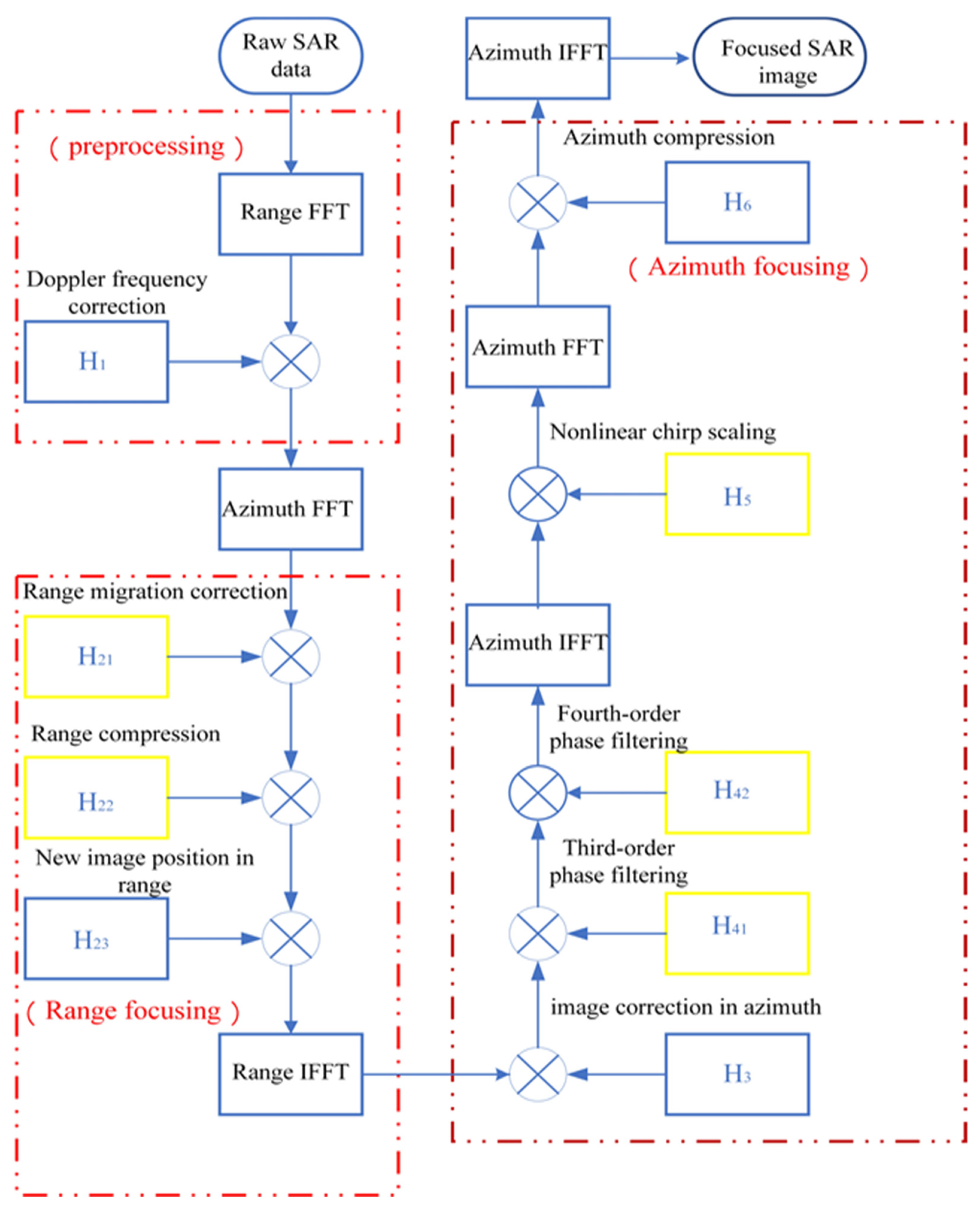
3. The Specific Steps of the Algorithm

The imaging method proposed in the paper was divided into the following four main steps. First, the Doppler frequency correction was performed in the range frequency azimuth time to obtain a corresponding spectrum in the next calculation. Second, the 2-D spectrum of spaceborne missile bistatic SAR echo signal was derived. Third, the operations in range complete range cell migration correction, range compression and determine the range direction position of the imaging scene. Finally, a modified NLCS algorithm was introduced to compensate for the azimuth FM rate, complete azimuth compression, and obtain the final image. According to Figure 3, the flowchart for the proposed algorithm was summarized to make each step of the process clear (the steps of algorithm improvement are marked with yellow boxes). The specific operations and derivations for each step are described in detail below.

3.1. Doppler Frequency Correction

Applying the range Fourier transform (FT) to (1) yields
S ( f r , η ) = w r ( f r ) w a ( η ) exp ( j π f r 2 k r ) exp ( j 2 π ( f r + f c ) c R ( η ) )
where f r represents the frequency domain variable corresponding to τ . Due to factors such as the missile’s own acceleration and forward-looking imaging that cause Doppler central frequency deviation, for later calculation in the two-dimensional spectrum, the spectrum needs to be shifted to the zero-frequency position. It is assumed that the motion parameters of the satellite and missile can be calculated accurately during operation. According to Formula (6), the Doppler central frequency is calculated as
f d = 2 λ d R ( η ) d η | η = 0 = 2 λ ( b 1 + k 1 x T v t x + y T v t y R T 0 v y y R + v z z R R R 0 )
The Doppler frequency deviation term x T v t x + y T v t y R T 0 v y y R + v z z R R R 0 needs to be corrected, and the Doppler frequency correction factor is
H 1 = exp ( j 2 π ( f r + f c ) c ( x T v t x + y T v t y R T 0 v y y R + v z z R R R 0 ) η ) ,
multiplying (7) and (5) in the range frequency and azimuth time domain yields
S 1 ( f r , η ) = w r ( f r ) w a ( η ) exp ( j π f r 2 k r ) exp [ j 2 π ( f r + f c ) c ( ( k 0 + b 0 ) + ( k 1 + b 1 ) η + ( k 2 + b 2 ) η 2 + ( k 3 + b 3 ) η 3 + ( k 4 + b 4 ) η 4 ) ] .

3.2. Derivation of the Signal 2-D Spectrum

Application of the azimuth Fourier transform to (8) needs to use the method of series reversion [20].
Assuming
S A ( f r , η ) = w r ( f r ) w a ( η ) exp ( j π f r 2 k r ) exp [ j 2 π ( f r + f c ) c R 1 ( η ) ] ,
where
R 1 ( η ) = ( k 0 + b 0 ) + ( k 2 + b 2 ) η 2 + ( k 3 + b 3 ) η 3 + ( k 4 + b 4 ) η 4 .
Then, applying the azimuth Fourier transform to (9) yields
S A ( f r , f a ) = w r ( f r ) w a ( f a ) exp ( j π f r 2 k r ) exp { j 2 π [ f c + f r c R 1 ( η ) + f a η ] } ,
where f a represents the frequency domain variable correspond to η . Substituting (10) into (11), assuming
Q ( η ) = 2 π ( f c + f r ) c ( ( k 2 + b 2 ) η 2 + ( k 3 + b 3 ) η 3 + ( k 4 + b 4 ) η 4 ) 2 π f a η ,
then
d Q d η = 2 π ( f c + f r ) c [ 2 ( k 2 + b 2 ) η + 3 ( k 3 + b 3 ) η 2 + 4 ( k 4 + b 4 ) η 3 ] 2 π f a = 0
From (13), we have
c ( f c + f r ) f a = 2 ( k 2 + b 2 ) η + 3 ( k 3 + b 3 ) η 2 + 4 ( k 4 + b 4 ) η 3 ,
applying the series reversion to (14) and inverting the power series yield
η = A 1 ( f a c f c + f r ) + A 2 ( f a c f c + f r ) 2 + A 3 ( f a c f r + f r ) 3 ,
where
A 1 = 1 2 ( k 2 + b 2 ) , A 2 = 3 ( k 3 + b 3 ) 8 ( k 2 + b 2 ) 3 , A 3 = 9 ( k 3 + b 3 ) 2 4 ( k 2 + b 2 ) ( k 4 + b 4 ) 16 ( k 2 + b 2 ) 5 .
Substituting (15) into (11), we obtain the 2-D spectrum of S A ( τ , η ) .
S A ( f r , f a ) = w r ( f r ) w a ( f a ) exp ( j π f r 2 k r ) exp { j 2 π φ 0 ( f r , f a ) } ,
where
φ 0 ( f r , f a ) = f c + f r c R 0 + A 1 2 ( k 2 + b 2 ) c A 1 c f c + f r f a 2 + ( A 2 + 2 A 1 A 2 ( k 2 + b 2 ) + A 1 3 ( k 3 + b 3 ) ) c 2 ( f c + f r ) 2 f a 3 + ( A 3 + 2 A 1 A 3 ( k 2 + b 2 ) + A 2 2 ( k 2 + b 2 ) + A 1 4 ( k 4 + b 4 ) + 3 A 1 2 A 2 ( k 3 + b 3 ) ) c 3 ( f c + f r ) 3 f a 4
According to the shift properties and FFT skew, we have
f ( τ , η ) F ( f τ , f η ) f ( τ , η ) exp { j 2 π f κ η } F ( f τ , f η + f κ ) f ( τ κ η , η ) F ( f τ , f η + κ f τ ) ,
then, we obtain the original 2-D point target spectrum
S 2 ( f r , f a ) = S A ( f r , f a + ( f c + f r ) k 1 + b 1 c ) = w r ( f r ) w a ( f a ) exp [ j φ ( f r , f a ) ] ,
where
φ ( f r , f a ) = π f r 2 K r 4 π ( f r + f c ) ( R T 0 + R R 0 ) c + 2 π c 8 b 2 ( f r + f c ) ( f a + 2 ( f r + f c ) c ( b 1 + k 1 ) ) 2 + 2 π ( b 3 + k 3 ) c 2 32 ( b 2 + k 2 ) 3 ( f r + f c ) 2 ( f a + 2 ( f r + f c ) c ( b 1 + k 1 ) ) 3 + 2 π ( 9 ( b 3 + k 3 ) 2 4 ( b 2 + k 2 ) ( b 4 + k 4 ) ) c 3 512 ( b 2 + k 2 ) 5 ( f r + f c ) 3 ( f a + 2 ( f r + f c ) c ( b 1 + k 1 ) ) 4 .
According to the properties of series convergence [34]
{ 1 f c + f r 1 f c ( 1 f r f c + f c 2 f c 2 f r 3 f c 3 ) 1 ( f c + f r ) 2 1 f c 2 ( 1 2 f r f c + 3 f r 2 f c 2 4 f r 3 f c 3 ) 1 ( f c + f r ) 3 1 f c 3 ( 1 3 f r f c + 6 f r 2 f c 2 10 f r 3 f c 3 ) ,
substituting (22) into (21) and expanding (21) into its Taylor series of f r at f r = 0 yields
φ ( f r , f a ) = φ 0 ( f a ) + φ 1 ( f a ) f r + φ 2 ( f a ) f r 2 + φ 3 ( f a ) f r 3 ,
where
φ 0 ( f a ) = 2 π f c c ( R T 0 + R R 0 ( b 1 + k 1 ) 2 4 ( b 2 + k 2 ) ( b 1 + k 1 ) 3 ( b 3 + k 3 ) 8 ( b 2 + k 2 ) 3 ( 9 ( b 3 + k 3 ) 2 4 ( b 2 + k 2 ) ( b 4 + k 4 ) ) ( b 1 + k 1 ) 4 64 ( b 2 + k 2 ) 5 ) + 2 π ( b 1 + k 1 2 ( b 2 + k 2 ) + 3 ( b 1 + k 1 ) 2 ( b 3 + k 3 ) 8 ( b 2 + k 2 ) 3 + ( 9 ( b 3 + k 3 ) 2 4 ( b 2 + k 2 ) ( b 4 + k 4 ) ) ( b 1 + k 1 ) 3 16 ( b 2 + k 2 ) 5 ) f a + 2 π ( c 4 ( b 2 + k 2 ) f c + 3 ( b 1 + k 1 ) ( b 3 + k 3 ) c 8 ( b 2 + k 2 ) 3 f c + ( 9 ( b 3 + k 3 ) 2 4 ( b 2 + k 2 ) ( b 4 + k 4 ) ) 3 ( b 1 + k 1 ) c 32 ( b 2 + k 2 ) 5 f c ) f a 2 + 2 π ( ( b 3 + k 3 ) c 2 8 ( b 2 + k 2 ) 3 f c 2 + ( 9 ( b 3 + k 3 ) 2 4 ( b 2 + k 2 ) ( b 4 + k 4 ) ) ( b 1 + k 1 ) c 2 16 ( b 2 + k 2 ) 5 f c 2 ) f a 3 + 2 π ( 9 ( b 3 + k 3 ) 2 4 ( b 2 + k 2 ) ( b 4 + k 4 ) ) c 3 64 ( b 2 + k 2 ) 5 f c 3 f a 4
φ 1 ( f a ) 2 π c ( ( R T 0 + R R 0 ) + ( b 1 + k 1 ) 2 4 ( b 2 + k 2 ) + ( b 1 + k 1 ) 3 ( b 3 + k 3 ) 8 ( b 2 + k 2 ) 3 + ( 9 ( b 3 + k 3 ) 2 4 ( b 2 + k 2 ) ( b 4 + k 4 ) ) ( b 1 + k 1 ) 4 64 ( b 2 + k 2 ) 5 ) 2 π ( c 4 ( b 2 + k 2 ) f c 2 + 3 ( b 1 + k 1 ) ( b 3 + k 3 ) c 8 ( b 2 + k 2 ) 3 f c 2 + ( 9 ( b 3 + k 3 ) 2 4 ( b 2 + k 2 ) ( b 4 + k 4 ) ) 3 ( b 1 + k 1 ) 3 c 32 ( b 2 + k 2 ) 5 f c 2 ) f a 2 2 π ( ( b 3 + k 3 ) c 2 4 ( b 2 + k 2 ) 3 f c 3 + ( 9 ( b 3 + k 3 ) 2 4 ( b 2 + k 2 ) ( b 4 + k 4 ) ) ( b 1 + k 1 ) c 2 16 ( b 2 + k 2 ) 5 f c 3 ) f a 3 2 π ( 9 ( b 3 + k 3 ) 2 4 ( b 2 + k 2 ) ( b 4 + k 4 ) ) 3 c 3 64 ( b 2 + k 2 ) 5 f c 4 f a 4 ,
φ 2 ( f a ) π K r + 2 π ( c 4 ( b 2 + k 2 ) f c 3 + 3 ( b 1 + k 1 ) ( b 3 + k 3 ) c 8 ( b 2 + k 2 ) 3 f c 3 + ( 9 ( b 3 + k 3 ) 2 4 ( b 2 + k 2 ) ( b 4 + k 4 ) ) 3 ( b 1 + k 1 ) 3 c 32 ( b 2 + k 2 ) 5 f c 3 ) f a 2 + 2 π ( 3 ( b 3 + k 3 ) c 2 8 ( b 2 + k 2 ) 3 f c 4 + ( 9 ( b 3 + k 3 ) 2 4 ( b 2 + k 2 ) ( b 4 + k 4 ) ) 3 ( b 1 + k 1 ) c 2 16 ( b 2 + k 2 ) f c 4 ) f a 3 + 2 π ( 9 ( b 3 + k 3 ) 2 4 ( b 2 + k 2 ) ( b 4 + k 4 ) ) 3 c 3 64 ( b 2 + k 2 ) 5 f c 5 f a 4 ,
φ 3 ( f a ) π c f a 2 2 f c 4 ( k 2 + b 2 ) 3 π c ( k 3 + b 3 ) ( k 1 + b 1 ) f a 2 4 f c 4 ( k 2 + b 2 ) 3 3 π c ( 9 ( k 3 + b 3 ) 3 4 ( k 2 + b 2 ) ( k 4 + b 4 ) ) ( k 1 + b 1 ) 2 f a 2 16 f c 4 ( k 2 + b 2 ) 5 π c 2 ( 9 ( k 3 + b 3 ) 2 4 ( k 2 + b 2 ) ( k 4 + b 4 ) ) ( k 1 + b 1 ) f a 3 2 f c 5 ( k 2 + b 2 ) 5 π c 2 ( k 3 + b 3 ) f a 3 f c 5 ( k 2 + b 2 ) 3 5 π c 3 ( 9 ( k 3 + b 3 ) 2 4 ( k 2 + b 2 ) ( k 4 + b 4 ) ) f a 4 16 f c 6 ( k 2 + b 2 ) 5
Inspecting (23), φ 0 ( f a ) represents the azimuth modulation, which has no correlation with range variables. φ 1 ( f a ) is the range frequency linear term coefficient, which is related to large range cell migration and can be matched with the corresponding filter to achieve linear range migration correction. The first component in φ 2 ( f a ) represents the range modulation, and the remainder of components are the secondary range compression (SRC) terms that represent the range–azimuth coupling. φ 3 ( f a ) is the cubic term of the range frequency, which represents the rate of change of the range chirp rate. Because of the range-dependent characteristic of the above formula, it is difficult to figure out an accurate compensation for all targets at different ranges. To solve this problem, it is necessary to analyze the range-dependent characteristic of the residual range cell migration (RCM) and SRC. Because the effect of higher order terms above, the third order is very small, and only the third term coefficients were considered.
The three points, T1, T6, and T16, are located at the position of range directions 0, 150 m, and 300 m, respectively, as shown in Figure 4. The range-dependent characteristic evaluation of the SRC and the residual RCM are shown in Figure 5. Observing the images, it can be seen that the SRC phase error and the residual RCM error were smaller than π / 4 and one range resolution cells, respectively. Thus, the imaging results would not be affected by those effects of the range dependence of the residual SRC and RCM.

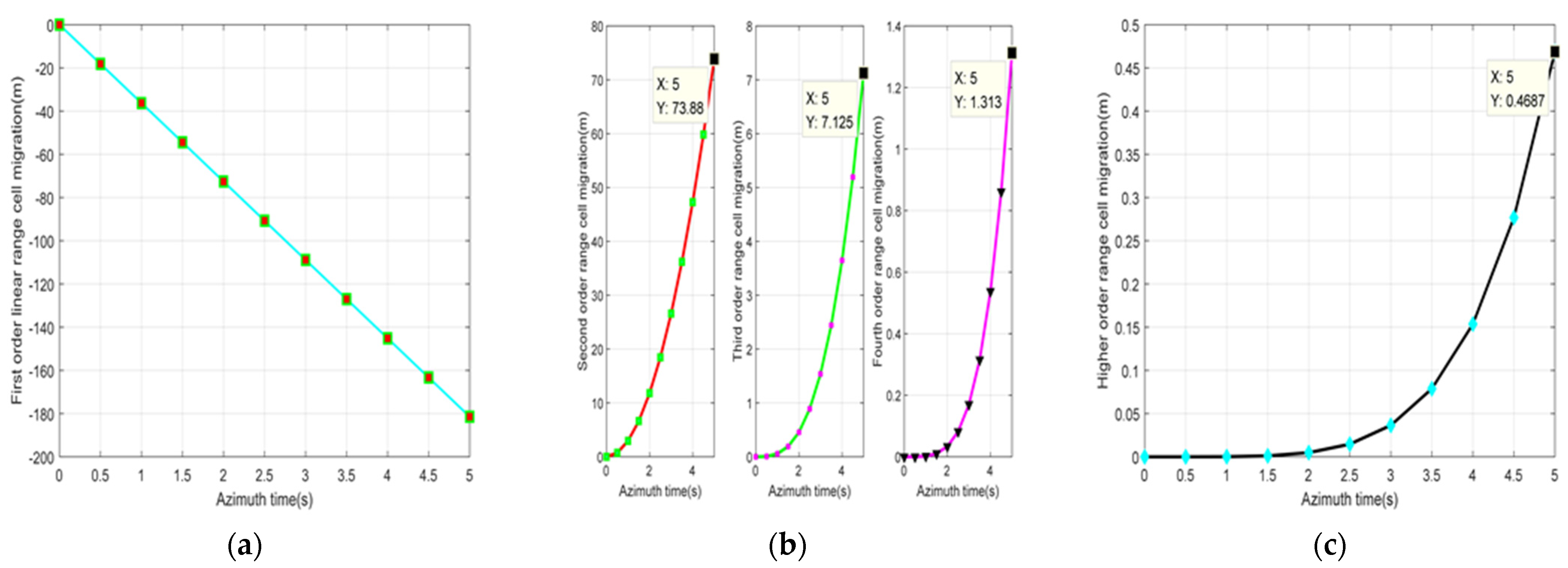
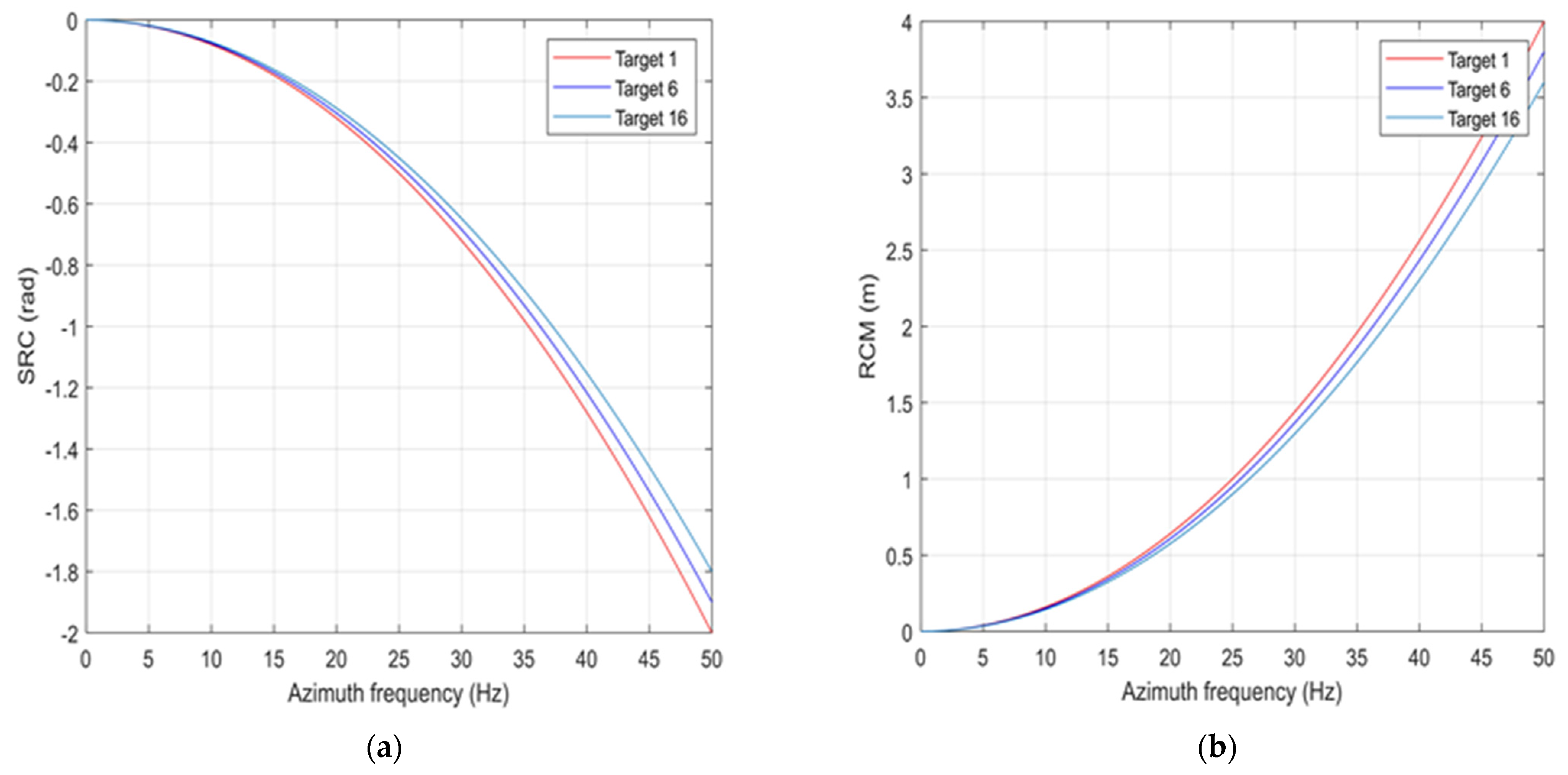
3.3. The Operations in Range

In order to keep the range migration error within 1/4 range sampling, we performed bulk range cell migration correction in the 2-D frequency domain by multiplying with the conjugate of φ 1 ( f a ) , setting the scene center as the reference point target. The factor was given by
H 21 = exp ( j φ 1 ( f a ) f r ) .
The range compression term is exp ( j φ 2 ( f a ) f r 2 ) . Because the missile was in the high-frequency band, only the first component term in φ 2 ( f a ) was kept, and the remainder terms in φ 2 ( f a ) . were ignored, having little impact on range compression. The range compression factor is expressed as
H 22 = π ( f r 2 / K r ) .
The echo signal of any point target in the scene will become a vertical line in the azimuth after range migration correction and range pulse compression. The linear term was eliminated after the range migration correction. In order to determine the range direction position of the imaging scene, the function was multiplied by
H 23 ( f r ) = exp { j 2 π f r c [ R T 0 + R R 0 ( b 1 + k 1 ) 2 4 ( b 2 + k 2 ) ( b 1 + k 1 ) 3 ( b 3 + k 3 ) 8 ( b 2 + k 2 ) 3 ( 9 ( b 3 + k 3 ) 2 4 ( b 2 + k 2 ) ( b 4 + k 4 ) ) ( b 1 + k 1 ) 4 64 ( b 2 + k 2 ) 5 ] } .
Multiplying (20) with (28), (29), (30) and transforming the result into range time azimuth frequency domain by the range inverse Fourier transform, the range focused signal can be written as
S 3 ( τ , f a ) = sin c [ B r ( τ R T R / c ) ] w a ( f a ) exp [ j φ 0 ( f a ) ] ,
where
R T R = R T 0 + R R 0 ( b 1 + k 1 ) 2 4 ( b 2 + k 2 ) ( b 1 + k 1 ) 3 ( b 3 + k 3 ) 8 ( b 2 + k 2 ) 3 ( 9 ( b 3 + k 3 ) 2 4 ( b 2 + k 2 ) ( b 4 + k 4 ) ) ( b 1 + k 1 ) 4 64 ( b 2 + k 2 ) 5 .
To illustrate the range processing of the aforementioned algorithm, some simulations on the echo trajectories and 2-D spectrum of the simulated targets are presented before and after the range operation, and the results are shown in Figure 6. The simulation parameters are shown in Table 1. Figure 6a shows the original signal in the time domain, Figure 6b represents the original signal in the two-dimensional frequency domain, Figure 6d is the image of the signal after range compression, Figure 6e is the image of the signal after range compression and migration correction, and Figure 6c shows the two-dimensional spectrum after range migration correction. Combined with the original signal echo in Figure 6a,d, the original signal echo was compressed into nine slanted straight lines after range compression, and then the slanted lines were straightened by range migration correction, as shown in Figure 6e. The spectrum was also corrected accordingly, as shown in Figure 6b,c.

3.4. Azimuth Compression by a Modified Bistatic Azimuth NLCS Algorithm

Different from the bistatic configuration with constant speed [28,29,30], after range pulse compression and range migration correction, the azimuth FM rate of the targets located in different azimuth directions of the same range unit changed significantly and could not be regarded as a constant (specific simulation analysis was conducted later). If the azimuthal direction is compressed directly by the azimuthal matching filter function, which is constructed by the azimuth FM rate of the azimuthal center, the edge target points of the imaging scene will be difficult to focus. Therefore, before the azimuth compression, the variation of azimuth FM rate along the azimuth direction must be compensated. The azimuth nonlinear scaling algorithm was introduced here to improve the effect of azimuth focusing.
The linear term coefficient of the azimuth frequency in the signal can be written as g ( y ) , which represents the azimuthal position of the target point.
g ( y ) = b 1 + k 1 2 ( b 2 + k 2 ) + 3 ( b 1 + k 1 ) 2 ( b 3 + k 3 ) 8 ( b 2 + k 2 ) 3 + ( 9 ( b 3 + k 3 ) 2 4 ( b 2 + k 2 ) ( b 4 + k 4 ) ) ( b 1 + k 1 ) 3 16 ( b 2 + k 2 ) 5 c
Expanding (32) into its Taylor series of y at y = 0 and keeping up to the first-order term yield
g ( y ) g 0 + ρ y ,
where
g 0 = g ( y ) | y = 0 = ( b 1 + k 1 2 ( b 2 + k 2 ) + 3 ( b 1 + k 1 ) 2 ( b 3 + k 3 ) 8 ( b 2 + k 2 ) 3 + ( 9 ( b 3 + k 3 ) 2 4 ( b 2 + k 2 ) ( b 4 + k 4 ) ) ( b 1 + k 1 ) 3 16 ( b 2 + k 2 ) 5 c ) | y = 0
ρ = d g ( y ) d y | y = 0 ,
g 0 represents the whole azimuth displacement, which is easily corrected by multiplying with its conjugate. ρ y reflects the compression or stretching of the image along the azimuth direction, which is caused by the acceleration and height speed. Due to the acceleration of the missile, the speed changes rapidly, making ρ y y / v y . In order to correct ρ y and make ρ y = y / v y , the nonlinear chirp scaling method proposed later was adopted to eliminate the influence on the image. First, the whole azimuth displacement g 0 was corrected by its conjugate factor as follows.
H 3 ( f a ) = exp ( j 2 π g 0 f a ) ,
multiplying (31) and (36) yields
S 4 ( τ , f a ) = sinc [ B r ( τ R T 0 + R R 0 c ) ] w a ( f a ) exp [ j ( θ + 2 π Δ η f a ) ] exp ( j π f a 2 K a ) exp ( j 2 π Z 1 f a 3 ) exp ( j 2 π Z 2 f a 4 ) ,
where
θ = 2 π ( 2 f c R T 0 c + ( b 1 + k 1 ) 2 f c 2 ( b 2 + k 2 ) c + ( b 1 + k 1 ) 3 ( b 3 + k 3 ) f c 4 ( b 2 + k 2 ) 3 c + ( 9 ( b 3 + k 3 ) 2 4 ( b 2 + k 2 ) ( b 4 + k 4 ) ) ( b 1 + k 1 ) 4 f c 32 ( b 2 + k 2 ) 5 c )
Δ η = ( b 1 + k 1 2 ( b 2 + k 2 ) + 3 ( b 1 + k 1 ) 2 ( b 3 + k 3 ) 8 ( b 2 + k 2 ) 3 + ( 9 ( b 3 + k 3 ) 2 4 ( b 2 + k 2 ) ( b 4 + k 4 ) ) ( b 1 + k 1 ) 3 16 ( b 2 + k 2 ) 5 c ) g 0
K a = 32 ( b 2 + k 2 ) 5 f c 8 ( b 2 + k 2 ) 4 c + 12 ( b 1 + k 1 ) ( b 2 + k 2 ) 2 ( b 3 + k 3 ) c + 3 ( b 1 + k 1 ) 2 c ( 9 ( b 3 + k 3 ) 2 4 ( b 2 + k 2 ) ( b 4 + k 4 ) )
Z 1 = ( b 3 + k 3 ) c 2 32 ( b 2 + k 2 ) 3 f c 2 + ( 9 ( b 3 + k 3 ) 2 4 ( b 2 + k 2 ) ( b 4 + k 4 ) ) ( b 1 + k 1 ) c 2 64 ( b 2 + k 2 ) 5 f c 2
Z 2 = ( 9 ( b 3 + k 3 ) 2 4 ( b 2 + k 2 ) ( b 4 + k 4 ) ) c 3 512 ( b 2 + k 2 ) 5 f c 3
Due to the influence of missile-borne acceleration, the azimuth FM rate mentioned above will change with the azimuth position y , as shown in Figure 7a. Considering the azimuth FM rate in the center of the scene as the whole azimuthal FM rate, it will dramatically affect the imaging focus on both sides of the scene edges. Therefore, it is very essential to perform a deep analysis in the azimuth-dependent characteristic of the azimuth FM rate. Expanding K a into its Taylor series of Δ η at Δ η = 0 yields
K a = K a 0 + K a 1 Δ η + K a 2 Δ η 2 + O ( Δ η ) ,
where
K a 0 = K a | Δ η = 0 , K a 1 = d K a d Δ η | Δ η = 0 = d K a d y | y = 0 d y d Δ η = 1 ρ d K a d y | y = 0
K a 2 = 1 2 d 2 K a d ( Δ η ) 2 | Δ η = 0 = 1 2 ρ d d Δ η ( d K a d y ) | Δ η = 0 = 1 2 ρ d 2 K a d y 2 | Δ η = 0 d y d Δ η = 1 2 ρ 2 d 2 K a d y 2 | y = 0
The third- and fourth-term coefficients Z 1 and Z 2 of f a in (37) had a small effect with the change of azimuth, as shown in Figure 7b, and for the convenience of calculation, the amplitude of variation can be ignored. Therefore, the coefficient amplitude of the whole azimuthal direction can be considered as the coefficient amplitude of the azimuthal center. Before the azimuth FM rate compensation and nonlinear chirp scaling operation, in order to eliminate the influence of the third-order and fourth-order terms of azimuth frequency f a , it is necessary to introduce the third-order and fourth-order filters in the range time azimuth frequency domain. The third-order and fourth-order were are as follows:
H 41 ( f a ) = exp ( j 2 π A f a 3 ) H 42 ( f a ) = exp ( j 2 π B f a 4 ) ,
where A and B are the uncertain parameters, which were calculated later.
Multiplying (37) with (39) yields
S 5 ( τ , f a ) = sinc [ B r ( τ R T 0 + R R 0 c ) / c ] w a ( f a ) exp ( j θ ) exp [ j ( 2 π Δ η f a π f a 2 / K a + 2 π A 1 f a 3 + 2 π B 1 f a 4 ) ] ,
where
A 1 = A + ( b 3 + k 3 ) c 2 32 ( b 2 + k 2 ) 3 f c 2 + ( 9 ( b 3 + k 3 ) 2 4 ( b 2 + k 2 ) ( b 4 + k 4 ) ) ( b 1 + k 1 ) c 2 64 ( b 2 + k 2 ) 5 f c 2 B 1 = B + ( 9 ( b 3 + k 3 ) 2 4 ( b 2 + k 2 ) ( b 4 + k 4 ) ) c 3 512 ( b 2 + k 2 ) 5 f c 3 .
Applying the principle of stationary phase (POSP) to (40) and transforming (40) into the azimuth time domain yields
S 6 ( τ , η ) = sinc [ B r ( τ R T 0 + R R 0 c ) ] w a ( η ) exp [ j π K a ( η Δ η ) 2 + j 2 π A 1 K a 3 ( η Δ η ) 3 ] exp [ j 2 π B 1 K a 4 ( η Δ η ) 4 ] .
The next step is to compensate the azimuth FM rate so that the azimuth FM rate of each target point is equal to the azimuth FM rate of the scene center. According to the algorithm of nonlinear chirp scaling, a fourth-order chirp scaling factor H 5 was constructed to multiply the above formula to meet the above requirements.
H 5 ( η ) = exp ( j π l 2 η 2 + j 2 π l 3 η 3 + j 2 π l 4 η 4 ) ,
where l 2 , l 3 , l 4 are the uncertain coefficients. Multiplying (42) with (43) and transforming the result into the azimuth frequency domain by applying the azimuth Fourier transform yields
S 7 ( τ , f a ) = w a ( f a ) sinc [ B r ( τ R T 0 + R R 0 c ) ] exp [ j ϕ ( f a ) ] ,
expressing the ϕ ( f a ) as a power series of Δ η and f a yields
ϕ ( f a ) = c 1 ( f a 2 , f a 3 , f a 4 ) + c 2 f a Δ η + c 3 f a Δ η 2 + c 4 f a 2 Δ η + c 5 f a 2 Δ η 2 + c 6 f a 3 Δ η + c 7 ( f a n Δ η m ) ,
where
{ c 1 = π K a 0 + l 2 f a 2 + 2 π A 1 K a 0 3 + l 3 ( K a 0 + l 2 ) 3 f a 3 + + 2 π B 1 K a 0 4 + l 4 ( K a 0 + l 2 ) 4 f a 4 c 2 = 2 π K a 0 K a 0 + l 2 c 3 = 2 π [ K a 1 K a 0 + l 2 + K a 0 K a 1 ( K a 0 + l 2 ) 2 + 3 A 1 K a 0 3 l 2 2 + 3 K a 0 2 l 3 ( K a 0 + l 2 ) 3 ] c 4 = π K a 1 ( K a 0 + l 2 ) 2 + 6 π A 1 K a 0 3 l 2 + K a 0 l 3 ( K a 0 + l 2 ) 3 c 5 = π K a 2 ( K a 0 + l 2 ) 2 + π 6 K a 1 l 3 K a 1 2 ( K a 0 + l 2 ) 3     18 π K a 0 K a 1 l 3 + A 1 K a 0 2 K a 1 l 2 2 ( K a 0 + l 2 ) 4 + 12 π K a 0 2 l 4 + B 1 K a 0 4 l 2 2 ( K a 0 + l 2 ) 4 c 6 = 6 π A 1 K a 0 2 K a 1 l 2 2 K a 1 l 3 + ( K a 0 + l 2 ) 4 + 8 π K a 0 l 4 B 1 K a 0 4 l 2 ( K a 0 + l 2 ) 4
As can be seen from (45), the first term contained only azimuth frequencies, which can be removed directly by constructing a conjugate-matching filter function during azimuth compression, while the second term is a linear term of azimuthal frequency, which contains the position information of the target imaging azimuth and cannot be removed. The remaining items represent the azimuth-dependent terms that degrade the effect of azimuth focusing. To compensate for the azimuth FM rate and eliminate azimuth-dependent modulation, making its value not change with azimuth position, we set c 2 ( l 2 ) to 2 π / α ( α = ρ v y ) and c 3 , c 4 , c 5 , c 6 , c 7 to 0. The formulas can be solved as follows.
{ A 1 = K a 1 ( α 0.5 ) 3 K a 0 3 ( α 1 ) , l 2 = K a 0 ( α 1 ) B 1 = 2 α K a 0 K a 2 + ( 10 α 5 ) K a 1 2 24 K a 0 5 ( α 1 ) ,   l 3 = K a 1 ( α 1 ) 6 l 4 = 2 α K a 0 K a 2 + ( 7 α 5 ) K a 1 2 24 K a 0 ,
substituting (47) into (44) yields
S 8 ( τ , f a ) = w a ( f a ) sinc [ B r ( τ R T 0 + R R 0 c ) ] exp ( j 2 π Δ η α f a j π 1 K a 0 + l 2 f a 2 ) exp [ j 2 π A 1 K a 0 3 + l 3 ( K a 0 + l 2 ) 3 f a 3 + j 2 π B 1 K a 0 4 + l 4 ( K a 0 + l 2 ) 4 f a 4 ] .
Inspecting (48), The second, third, and fourth term coefficients of azimuth frequency are constant and no longer vary with azimuthal change, and thus the compensation correction was completed and the azimuth-dependent characteristic of the azimuth FM rate was removed entirely. Therefore, the azimuth direction can be compressed directly, and the azimuth matching filter function can be written as
H 6 ( f a ) = exp [ j π 1 K a 0 + l 2 f a 2 j 2 π A 1 K a 0 3 + l 3 ( K a 0 + l 2 ) 3 f a 3 j 2 π B 1 K a 0 4 + l 4 ( K a 0 + l 2 ) 4 f a 4 ] ,
multiplying (48) with (49) yields
S 9 ( τ , f a ) = sinc [ B r ( τ R T 0 + R R 0 c ) ] w a ( f a ) exp ( j 2 π Δ η α f a ) .
Transforming (50) into the range time azimuth time domain by azimuth inverse FT yields the final SAR image.

4. Experimental Simulations and Discussion

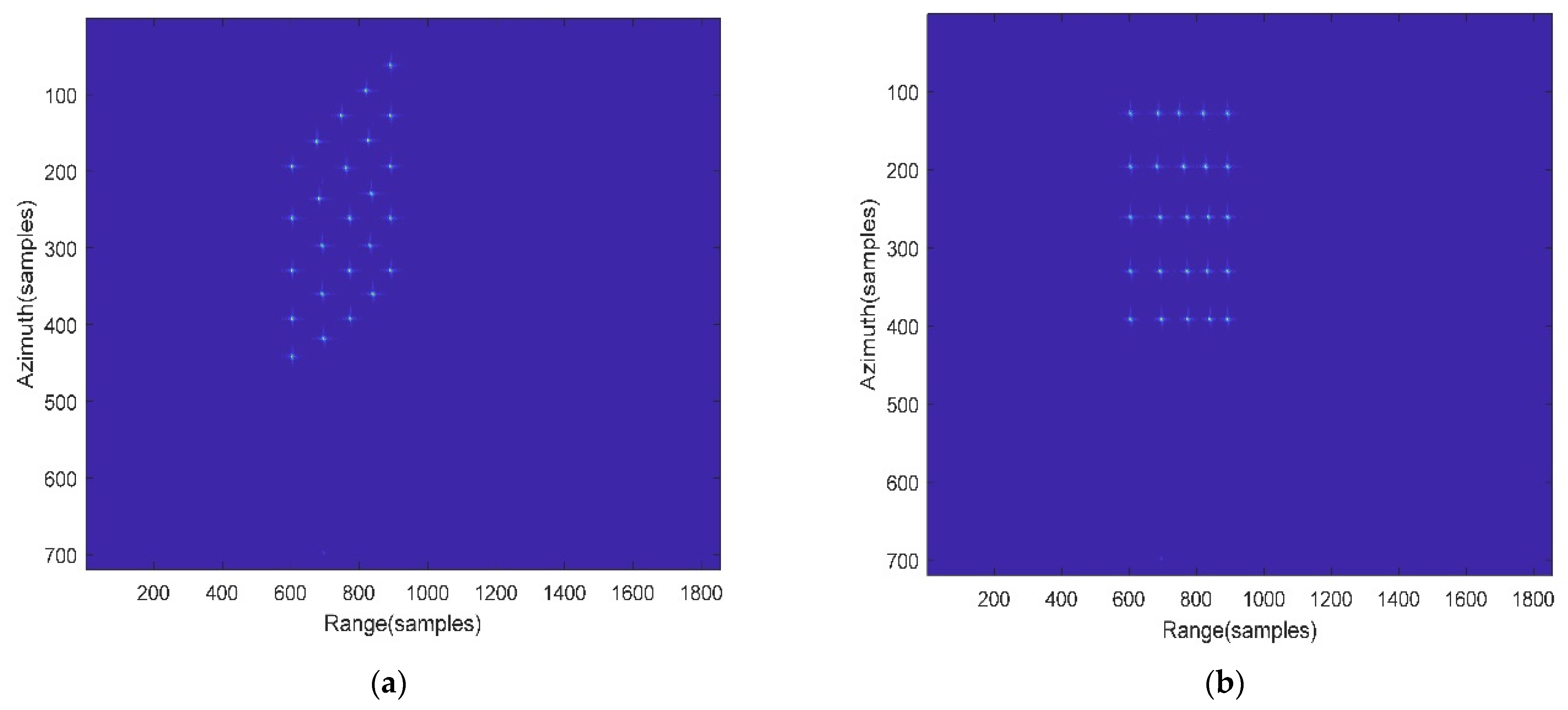
4.1. Simulation Results by the Proposed Algorithm

As shown in Figure 4, the simulations chose an array of 5 × 5 point targets at intervals of 100 m and 150 m in the azimuth and range axes, respectively. T1 is the target point at the center of the scene, and T5 is the edge point with the most severe azimuthal variation. The system parameters used in the simulation are shown in Table 1. The results of the point target imaging simulation are shown in Figure 8a. Due to the influence of forward-looking imaging, there was a certain geometric distortion in the range and azimuth direction, which was not consistent with the real target position. The results of the distortion correction are shown in Figure 8b.

4.2. Comparison of Algorithm Efficiency

As can be seen from the flow chart, the increase in the computation of the algorithm mainly came from the azimuth nonlinear scaling operations, including one FFT, one IFFT, and five times phase multiplication (as shown in the azimuth-processing section of the flow chart). According to [6], a complex phase multiplication takes six FLOPs, and an N-point FFT or IFFT takes 5 N log 2 ( N ) FLOPs [35]. In the simulation experiment, the number of sampling points in the range direction was N f a s t = 2048 , the number of sampling points in the azimuth direction was N s l o w = 512 , and the number of output points selected after range compression was N r = 1856 . It can be calculated that the added floating point arithmetic amount after the azimuth nonlinear operation was
Δ Q = 2 × 5 N r N s l o w log 2 ( N s l o w ) + 5 × 6 N r N s l o w = 0.950272 × 10 6 ( FLOPs )
Although the calculation amount was slightly increased compared with that without considering the space variance of azimuth FM rate, the azimuthal focusing was obviously improved and the image effect was better.
The computational complexity of the traditional NLCS algorithm in [36] was (setting the interpolation kernel value to 6)
Q 1 = 20 N s l o w N r log 2 N r + 20 N s l o w N r log 2 N s l o w + 30 N a N r + 2 ( 2 N k 1 ) N a N r = 4.26824171 × 10 8 ( FLOPs ) ,
the total computation of the proposed algorithm in this paper is
Q = 2 × 5 N r N s l o w log 2 ( N r ) + 4 × 5 N r N s l o w log 2 ( N s l o w ) + 9 × 6 N r N s l o w = 3.25544181 × 10 8 ( FLOPs )
It can be seen that the computational amount of the algorithm proposed in this paper was better than the traditional NLCS algorithm in [36], and the algorithm in this paper had no time-consuming interpolation operation, and thus its processing efficiency was higher. Moreover, the azimuth focusing was significantly improved, and the image effect was better (a detailed comparison is made in the next section).

4.3. Comparison of Imaging Effects

In order to evaluate the imaging performance of the proposed method, the traditional azimuth NLCS algorithm in [36] was introduced here to process the same simulated data, which solely considered the linear component of azimuth FM rate and disregarded the effects of residual RCM. Figure 9b shows the imaging result obtained by the traditional azimuth NLCS algorithm. By comparing Figure 9a,b, it can be seen that the traditional azimuth NLCS algorithm failed to achieve the same focus on the azimuth direction as the proposed azimuth NLCS algorithm because of the mismatched azimuth FM rate. The imaging result of point 1, point 3, and point 5 that were positioned at the same range but in different azimuth directions are shown in Figure 9a,b by using the traditional azimuth NLCS algorithm and the proposed azimuth NLCS algorithm, respectively. By comparing Figure 9a,b, it can be seen that in Figure 9a, the imaging effect was good with the change of azimuth distance from the center of the scene to the edge of the scene, while in Figure 9b, the image quality in the azimuth direction decreased rapidly. The specific performance comparison of imaging results is shown in Figure 10. Furthermore, Table 2 shows the calculated PSLR and ISLR for the corresponding targets in order to evaluate the imaging performance of the proposed NLCS algorithm. According to the Table 2, the proposed NLCS algorithm achieved nearly theoretical PSLR and ISLR, whereas the traditional NLCS was only able to achieve focused performance in the range direction, and in azimuth direction, the measured parameters were poorer than the theoretical values.

5. Conclusions

In this paper, a modified NLCS algorithm for the spaceborne missile bistatic SAR data processing is presented. Firstly, the system configuration and signal model were established, and then the Doppler frequency correction was carried out to eliminate Doppler center frequency deviation, which was caused by the acceleration of the missile itself and the forward-looking imaging. Next, the two-dimensional spectrum expression was derived by the method of series reversion, and range migration correction and range compression were performed in the two-dimensional frequency domain. Then, a modified azimuth NLCS operation was applied to eliminate the azimuth dependence of Doppler parameters through the use of a higher order approximation to the cubic phase term and azimuth FM rate. The modified azimuth NLCS operation equalized the azimuth FM rate so that azimuth compression can be achieved. Finally, the high efficiency and feasibility of the algorithm were proved by comparing the imaging effect, computational efficiency, and performance analysis between different algorithms.

Author Contributions

Conceptualization, Z.X. and W.Z.; methodology, Z.X.; software, Z.X. and W.Z; validation, Z.X., W.Z. and C.L.; formal analysis, Z.X.; investigation, D.L.; resources, D.L. and C.L; data curation, Z.X.; writing—original draft preparation, Z.X.; writing—review and editing, C.D. and T.H.; visualization, H.W.; supervision, C.D.; project administration, C.D. and T.H.; funding acquisition, C.D. and C.L. All authors have read and agreed to the published version of the manuscript.

Funding

This work was supported in part by the National Project Funding under Grant 2019-JCJQ-ZD-076-00.

Data Availability Statement

Not applicable.

Acknowledgments

The authors would like to thank all editors and reviewers for their comments on this paper.

Conflicts of Interest

The authors declare no conflict of interest.

References

  1. Cruz, H.; Véstias, M.; Monteiro, J.; Neto, H.; Duarte, R.P. A Review of Synthetic-Aperture Radar Image Formation Algorithms and Implementations: A Computational Perspective. Remote Sens. 2022, 14, 1258. [Google Scholar] [CrossRef]
  2. Cui, C.; Dong, X.; Chen, Z.; Hu, C.; Tian, W. A Long-Time Coherent Integration STAP for GEO Spaceborne-Airborne Bistatic SAR. Remote Sens. 2022, 14, 593. [Google Scholar] [CrossRef]
  3. Li, Q.; Zhang, Y.; Wang, Y.; Bai, Y.; Zhang, Y.; Li, X. Numerical Simulation of SAR Image for Sea Surface. Remote Sens. 2022, 14, 439. [Google Scholar] [CrossRef]
  4. Li, Z.; Huang, C.; Sun, Z.; An, H.; Wu, J.; Yang, J. BeiDou-based passive multistatic radar maritime moving target detection technique via space–time hybrid integration processing. IEEE Trans. Geosci. Remote Sens. 2021, 60, 5802313. [Google Scholar] [CrossRef]
  5. Sun, Z.; Wu, J.; Li, Z.; An, H.; He, X. Geosynchronous spaceborne–airborne bistatic SAR data focusing using a novel range model based on one-stationary equivalence. IEEE Trans. Geosci. Remote Sens. 2020, 59, 1214–1230. [Google Scholar] [CrossRef]
  6. Li, C.; Zhang, H.; Deng, Y.; Wang, R.; Liu, K.; Liu, D.; Jin, G.; Zhang, Y. Focusing the L-band spaceborne bistatic SAR mission data using a modified RD algorithm. IEEE Trans. Geosci. Remote Sens. 2019, 58, 294–306. [Google Scholar] [CrossRef]
  7. Chen, Z.; Tang, S.; Ren, Y.; Guo, P.; Zhou, Y.; Huang, Y.; Wan, J.; Zhang, L. Curvilinear Flight Synthetic Aperture Radar (CF-SAR): Principles, Methods, Applications, Challenges, and Trends. Remote Sens. 2022, 14, 2983. [Google Scholar] [CrossRef]
  8. Chen, P.; Zuo, L.; Wang, W. Adaptive Beamforming for Passive Synthetic Aperture with Uncertain Curvilinear Trajectory. Remote Sens. 2021, 13, 2562. [Google Scholar] [CrossRef]
  9. Huang, P.; Xia, X.-G.; Wang, L.; Xu, H.; Liu, X.; Liao, G.; Jiang, X. Imaging and relocation for extended ground moving targets in multichannel SAR-GMTI systems. IEEE Trans. Geosci. Remote Sens. 2021, 60, 5214024. [Google Scholar] [CrossRef]
  10. Jiang, C.; Tang, S.; Ren, Y.; Li, Y.; Zhang, J.; Li, G.; Zhang, L. Three-Dimensional Coordinate Extraction Based on Radargrammetry for Single-Channel Curvilinear SAR System. Remote Sens. 2022, 14, 4091. [Google Scholar] [CrossRef]
  11. Loffeld, O.; Nies, H.; Peters, V.; Knedlik, S. Models and useful relations for bistatic SAR processing. IEEE Trans. Geosci. Remote Sens. 2004, 42, 2031–2038. [Google Scholar] [CrossRef]
  12. Guo, Z.; Fu, Z.; Chang, J.; Wu, L.; Li, N. A Novel High-Squint Spotlight SAR Raw Data Simulation Scheme in 2-D Frequency Domain. Remote Sens. 2022, 14, 651. [Google Scholar] [CrossRef]
  13. Wang, R.; Loffeld, O.; Ul-Ann, Q.; Nies, H.; Ortiz, A.M.; Samarah, A. A bistatic point target reference spectrum for general bistatic SAR processing. IEEE Geosci. Remote Sens. Lett. 2008, 5, 517–521. [Google Scholar] [CrossRef]
  14. Vu, V.T.; Sjögren, T.K.; Pettersson, M.I. Two-dimensional spectrum for BiSAR derivation based on Lagrange inversion theorem. IEEE Geosci. Remote Sens. Lett. 2013, 11, 1210–1214. [Google Scholar] [CrossRef] [Green Version]
  15. Natroshvili, K.; Loffeld, O.; Nies, H.; Ortiz, A.M.; Knedlik, S. Focusing of general bistatic SAR configuration data with 2-D inverse scaled FFT. IEEE Trans. Geosci. Remote Sens. 2006, 44, 2718–2727. [Google Scholar] [CrossRef]
  16. Wang, R.; Loffeld, O.; Nies, H.; Knedlik, S.; Ender, J.H. Chirp-scaling algorithm for bistatic SAR data in the constant-offset configuration. IEEE Trans. Geosci. Remote Sens. 2008, 47, 952–964. [Google Scholar] [CrossRef]
  17. Zhang, X.; Yang, P.; Dai, X. Focusing multireceiver SAS data based on the fourth-order legendre expansion. Circ Syst Signal Pr. 2019, 38, 2607–2629. [Google Scholar] [CrossRef]
  18. Bie, B.; Quan, Y.; Sun, G.-C.; Liu, W.; Xing, M. A modified range model and Doppler resampling based imaging algorithm for high squint SAR on maneuvering platforms. IEEE Geosci. Remote Sens. Lett. 2019, 17, 1923–1927. [Google Scholar] [CrossRef]
  19. Deng, Y. Focus Improvement of Airborne High-Squint Bistatic SAR Data Using Modified Azimuth NLCS Algorithm Based on Lagrange Inversion Theorem. Remote Sens. 2021, 13, 1916. [Google Scholar]
  20. Neo, Y.L.; Wong, F.; Cumming, I.G. A two-dimensional spectrum for bistatic SAR processing using series reversion. IEEE Geosci. Remote Sens. Lett. 2007, 4, 93–96. [Google Scholar] [CrossRef] [Green Version]
  21. Yuan, Y.; Chen, S.; Zhao, H. An improved RD algorithm for maneuvering bistatic forward-looking SAR imaging with a fixed transmitter. Sensors 2017, 17, 1152. [Google Scholar] [CrossRef] [PubMed]
  22. Huang, L.; Qiu, X.; Hu, D.; Ding, C. Focusing of medium-earth-orbit SAR with advanced nonlinear chirp scaling algorithm. IEEE Trans. Geosci. Remote Sens. 2010, 49, 500–508. [Google Scholar] [CrossRef]
  23. Pu, W.; Li, W.; Lv, Y.; Wang, Z. An extended omega-K algorithm with integrated motion compensation for bistatic forward-looking SAR. In Proceedings of the 2015 IEEE Radar Conference (RadarCon), Arlington, VA, USA, 10–15 May 2015; pp. 1291–1295. [Google Scholar]
  24. Wu, S.; Xu, Z.; Wang, F.; Yang, D.; Guo, G. An improved back-projection algorithm for GNSS-R BSAR imaging based on CPU and GPU platform. Remote Sens. 2021, 13, 2107. [Google Scholar] [CrossRef]
  25. Zhang, H.; Tang, J.; Wang, R.; Deng, Y.; Wang, W.; Li, N. An accelerated backprojection algorithm for monostatic and bistatic SAR processing. Remote Sens. 2018, 10, 140. [Google Scholar] [CrossRef] [Green Version]
  26. Yu, M.; Zhang, X.; Liu, Z. Acceleration of fast factorized back projection algorithm for bistatic SAR. In Proceedings of the 2013 IEEE International Geoscience and Remote Sensing Symposium-IGARSS, Melbourne, Australia, 21–26 July 2013; pp. 2493–2496. [Google Scholar]
  27. Kitamura, T.; Kageme, S.; Suwa, K. Study on Three-Dimensional Fast Factorized Back Projection Using One-Dimensional Bistatic Antenna Array for Security Radar. In Proceedings of the 2021 7th Asia-Pacific Conference on Synthetic Aperture Radar (APSAR), Bali Island, Indonesia, 1–5 November 2021; pp. 1–6. [Google Scholar]
  28. Qiu, X.; Hu, D.; Ding, C. An improved NLCS algorithm with capability analysis for one-stationary BiSAR. IEEE Trans. Geosci. Remote Sens. 2008, 46, 3179–3186. [Google Scholar] [CrossRef]
  29. Wong, F.; Yeo, T.S. New applications of nonlinear chirp scaling in SAR data processing. IEEE Trans. Geosci. Remote Sens. 2001, 39, 946–953. [Google Scholar] [CrossRef]
  30. Chen, S.; Zhang, S.; Zhao, H.; Zhou, X.; Chen, Y. Improved nonlinear chirp scaling algorithm for dechirped missile-borne synthetic aperture radar. J. Appl. Remote Sens. 2014, 8, 083505. [Google Scholar] [CrossRef]
  31. Zhao, S.; Deng, Y.; Wang, R. Imaging for high-resolution wide-swath spaceborne SAR using cubic filtering and NUFFT based on circular orbit approximation. IEEE Trans. Geosci. Remote Sens. 2016, 55, 787–800. [Google Scholar] [CrossRef]
  32. Dong, X.; Sui, Y.; Li, Y.; Chen, Z.; Hu, C. Modeling and Analysis of RFI Impacts on Imaging between Geosynchronous SAR and Low Earth Orbit SAR. Remote Sens. 2022, 14, 3048. [Google Scholar] [CrossRef]
  33. Sun, Z.; Wu, J.; Pei, J.; Li, Z.; Huang, Y.; Yang, J. Inclined geosynchronous spaceborne–airborne bistatic SAR: Performance analysis and mission design. IEEE Trans. Geosci. Remote Sens. 2015, 54, 343–357. [Google Scholar] [CrossRef]
  34. Neo, Y.L.; Wong, F.H.; Cumming, I.G. Processing of azimuth-invariant bistatic SAR data using the range Doppler algorithm. IEEE Trans. Geosci. Remote Sens. 2007, 46, 14–21. [Google Scholar] [CrossRef]
  35. Li, D.; Lin, H.; Liu, H.; Liao, G.; Tan, X. Focus improvement for high-resolution highly squinted SAR imaging based on 2-D spatial-variant linear and quadratic RCMs correction and azimuth-dependent Doppler equalization. IEEE J. Sel. Top. Appl. Earth Obs. Remote Sens. 2016, 10, 168–183. [Google Scholar] [CrossRef]
  36. Wong, F.H.; Cumming, I.G.; Neo, Y.L. Focusing bistatic SAR data using the nonlinear chirp scaling algorithm. IEEE Trans. Geosci. Remote Sens. 2008, 46, 2493–2505. [Google Scholar] [CrossRef]
Figure 1. Geometry configuration of spaceborne missile bistatic SAR.
Remotesensing 14 05770 g001
Figure 2. Each order term of the range cell migration. (a) The first-order term; (b) from the second-order to the fourth-order term; (c) the high-order term.
Remotesensing 14 05770 g002
Figure 3. Flow chart of the proposed algorithm.
Remotesensing 14 05770 g003
Figure 4. Positions of the 25-point targets in the imaging region.
Remotesensing 14 05770 g004
Figure 5. The range-dependent characteristic evaluation of the SRC and the residual RCM. (a) SRC phase of T1, T6, and T16; (b) RCM of T1, T6, and T16.
Remotesensing 14 05770 g005
Figure 6. Illustration of the range operation in the proposed algorithm. (a) The original signal in the time domain; (b) the original signal in the two-dimensional frequency domain; (c) the two-dimensional spectrum after range migration correction; (d) the image of the signal after range compression; (e) the image of the signal after range compression and migration correction.
Remotesensing 14 05770 g006
Figure 7. The amplitude varies with azimuth direction. (a) The azimuth frequency modulation rate; (b) Z 1 and Z 2 .
Remotesensing 14 05770 g007
Figure 8. Final imaging results. (a) Before deformity correction; (b) after deformity correction.
Remotesensing 14 05770 g008
Figure 9. Imaging results of T1, T3, and T5 points using the imaging algorithm. (a) The proposed algorithm; (b) the traditional algorithm.
Remotesensing 14 05770 g009aRemotesensing 14 05770 g009b
Figure 10. Detailed imaging results by the traditional NLCS and modified algorithm. (a) Contour plot of target 1 focused by the modified algorithm. (b) Azimuth impulse responses of target 1 by the modified algorithm. (c) Range impulse responses of target 1 by the modified algorithm. (d) Contour plot of target 1 focused by the traditional NLCS algorithm. (e) Azimuth impulse responses of target 1 by the traditional NLCS algorithm. (f) Range impulse responses of target 1 by the traditional NLCS algorithm. (g) Contour plot of target 3 focused by the modified algorithm. (h) Azimuth impulse responses of target 3 by the modified algorithm. (i) Range impulse responses of target 3 by the modified algorithm. (j) Contour plot of target 3 focused by the traditional NLCS algorithm. (k) Azimuth impulse responses of target 3 by the traditional NLCS algorithm. (l) Range impulse responses of target 3 by the traditional NLCS algorithm. (m) Contour plot of target 5 focused by the modified algorithm. (n) Azimuth impulse responses of target 5 by the modified algorithm. (o) Range impulse responses of target 5 by the modified algorithm. (p) Contour plot of target 5 focused by the traditional NLCS algorithm. (q) Azimuth impulse responses of target 5 by the traditional NLCS algorithm. (r) Range impulse responses of target 5 by the traditional NLCS algorithm.
Remotesensing 14 05770 g010aRemotesensing 14 05770 g010bRemotesensing 14 05770 g010c
Table 1. Simulation experimental parameters of spaceborne missile bistatic SAR.
Simulation Experimental ParametersTransmitter Receiver
Velocity in x-direction5200 m/s
Velocity in y-direction−5200 m/s 100 m/s
Velocity in z-direction −50 m/s
Acceleration in y-direction 10 m/s2
Acceleration in z-direction −10 m/s2
Initial coordinate(280, 280, 755) km (0, 10, 5) km
Signal bandwidth 80 MHz
Pulse width 10 μs
Carrier frequency 5.4 GHz
Azimuth sampling interval 0.001 s
Synthetic aperture time 5 s
Range sampling frequency 160 MHz
Table 2. The imaging performance index of different algorithms.
Method AzimuthRange
TargetResolution(m)PSLR(dB)ISLR(dB)Resolution(m)PSLR(dB)ISLR(dB)
Modified NLCS algorithmT11.09−13.55−9.611.83−13.21−10.34
T31.12−13.26−9.521.86−13.12−10.21
T51.21−12.96−9.481.88−13.18−10.03
Traditional NLCS algorithmT11.13−12.98−9.501.84−12.96−10.10
T31.52−10.87−8.521.88−12.87−9.97
T52.08−9.64−7.691.90−12.90−9.89
Publisher’s Note: MDPI stays neutral with regard to jurisdictional claims in published maps and institutional affiliations.

