SAR Image Simulation Based on Effective View and Ray Tracing

Abstract

We present a novel echo-based synthetic aperture radar (SAR) image simulation method that comprehensively utilizes both SAR effective view and ray tracing algorithms. To improve the fidelity of simulated SAR images, we first design an SAR effective view algorithm to process the selected facet target model, with the purpose of discretizing the facets in the SAR effective view into lattice targets and ensuring that the interval of lattice targets is set strictly following the Nyquist sampling law. Then, we combine the ray tracing algorithm and SAR echo time-domain simulation and perform SAR echo time-domain simulation of lattice targets based on ray tracing. Various kinds of backscatter coefficient for each point target can be recorded, corresponding to the number of transmitted pulses within the synthetic aperture time. The echo matrixes of lattice targets are superimposed to generate the raw echo signal. Finally, the raw echo signal is processed by using the range-Doppler (RD) imaging algorithm to obtain the simulated SAR image. We conducted SAR image simulation tests on several facet target models, including car body, assault boat, and airplane, with different material properties. The simulated SAR images obtained by the proposed method were qualitatively and quantitatively evaluated. The experimental results verify the effectiveness of the proposed method.

1. Introduction

SAR techniques have increasingly been applied in various fields, such as military reconnaissance, ocean research, and environmental remote sensing. With the rapid development of SAR techniques, new systems are constantly being developed. Due to the low cost and easy operation of the SAR image simulation method, it has been widely used in several steps of SAR system development. In particular, the echo-based SAR image simulation method can reproduce the actual working process of SAR systems and has become a powerful tool in SAR system design, algorithm testing, and system verification. Simulated SAR images are also essential for establishing noncooperative target datasets [1,2,3].

Some studies on echo-based SAR image simulation have been conducted, and can be approximately classified into two categories. The first is SAR image simulation for system development, and the other is simulation for a specific echo simulation mechanism. System development-oriented research mainly focuses on the coordination of the various subsystem modules. Some representative SAR simulation systems have been proposed. For instance, the Franceschetti team developed a three-dimensional distributed target SAR simulator (SARAS), which is a relatively mature SAR simulator [4,5,6]. Horn et al. designed an airborne simulation system (E-SAR) for SAR system performance analysis to evaluate the rationality of SAR system parameter design [7]. Boerner et al. introduced an SAR simulator (SARIS), mainly to reduce the test cost of setting the actual system parameters of SAR [8]. Margarit et al. proposed a SAR simulator for generating polarimetric SAR and polarimetric inverse SAR data for complex targets, which can solve electromagnetic problems through high-frequency approximations such as physical optics [9]. Min et al. designed an application-oriented spaceborne SAR advanced simulator (SBRAS), which developed a complete signal processing flow, including SAR raw data simulation of natural scenes, imaging, and interferometric SAR (InSAR) processing [10]. Dumont et al. proposed a SAR simulator (DIONISOS) with a three-dimensional GUI environment, including modules of electromagnetic models and related material properties [11]. Klaus et al. built a SAR system simulator (SiSAR) including target model modeling, echo simulation, and imaging functions. [12]. Speck et al. developed a spaceborne SAR simulator (SETES), which can simulate hardware platform information, analyze system errors, and evaluate imaging results [13]. Mori et al. proposed a multimode spaceborne interferometric SAR echo simulator [14]. Allan et al. summarized the theory and functions of a time-domain SAR system simulator (CSAR), including simulating arbitrary trajectories of moving targets, SAR platforms, and antenna configurations [15]. Drozdowicz developed an open-source SAR simulation framework that can be used for a variety of purposes and is a powerful tool for developing SAR simulation systems [16]. Ilyushin et al. introduced a SAR simulation system (CLUSIM), which conducted echo simulation experiments using real planetary surface topography datasets [17]. Martion et al. designed a SAR signal simulator (Pol-SARAS) that could simulate the original signal of multiple polarization channels simultaneously [18]. However, most of the above studies mainly focused on the coordination of the various subsystem modules. As listed above, each SAR simulator is designed for specific application scenarios. With the continuous development of new SAR systems, the methods of the existing SAR simulation system submodules are lagging behind. In recent years, many new SAR image simulation methods have been proposed based on the above representative SAR system simulation engineering techniques.

Compared to system development-oriented research, echo simulation mechanism-oriented research mainly simulates the mechanism of images, focusing on how radar electromagnetic waves interact with target objects. Some effective echo-based SAR image simulation methods have been proposed. Franceschetti’s team carried out a systematic study on the rapid simulation method of SAR raw data and proposed a simulation method based on a two-dimensional frequency domain. Subsequently, they proposed a hybrid strip-spot SAR echo simulation method and carried out echo simulation for extended targets [19,20,21,22,23,24]. The echo time-domain simulation method was proposed by Kaupp and Pike. The time-domain method calculated the echo signal of each scattering unit in the scene completely, according to the order of the time-domain transmitted pulse, so the echo phase had high precision [25]. Takero et al. obtained an SAR image of a time-varying sea surface based on the time-domain echo simulation method [26]. The physical optics (PO) method in electromagnetism theory was used to calculate the backscatter coefficient of the target, and the ray tracing method was used to address the problem that the target was occluded to form a shadow [27]. Tao et al. proposed an SAR simulation technique for target recognition in complex urban backgrounds [28]. Aiming at the time and space variability of the target backscatter coefficient, the finite difference time domain (FDTD) was used to calculate the backscatter coefficient of the target point, which improves the accuracy of echo time-domain simulation [29]. Fan et al. briefly introduced the multimode Gaofen-3 SAR simulation system framework and used the echo time-domain simulation method to simulate the original data [30]. The shooting bouncing ray (SBR) method was used to calculate the backscatter coefficient of the target and the geometrical optics (GO) method was used to track the energy propagation path, and a good SAR image simulation effect was obtained [31]. Qian et al. proposed a time-varying sea surface imaging numerical simulation method based on the echo signal, which was helpful for SAR imaging research [32].

The above studies have achieved good results in SAR image simulation, but they are still limited when applied in different application scenarios. In particular, some methods assume that the backscatter coefficient of the target point is invariant within the synthetic aperture time and directly use the existing SAR images as a backscatter matrix for echo simulation. Some improved methods evaluated only single scattering and handled facet occlusion relationships based on micro-surface theory. These methods simplify the conditions affecting the calculation of the backscatter coefficient. The accuracy of the simulated echo signal is critical to the fidelity of the simulated SAR image. The backscatter coefficient is the most critical component of the SAR echo signal. To address the above issues, some representative studies have also proposed SAR echo-based simulation methods, including multiple scattering and electromagnetic scattering calculations, which have a good effect on ensuring the authenticity of the backscatter coefficient. However, their performance is still limited when handling the facet occlusion relationship of the target model. Some methods do not strictly follow the actual SAR working system mode to obtain the facets of the model in the SAR effective view. The occlusion judgment of facets is still carried out by the rendering methods of the traditional computer graphics field. In addition, when addressing targets with electrically large sizes, some commercial electromagnetic scattering calculation software, such as FEKO and CST, are usually used, and high-frequency approximation or high-frequency mixed related methods are used to calculate the backscatter coefficient. These methods propose many ideal assumptions in the calculation process, and the optional test parameters of material properties are limited. The above details affect the authenticity of the backscatter coefficient.

To address the aforementioned limitations, this paper proposes a novel echo-based SAR image simulation method based on both SAR effective view and ray tracing algorithms. First, we design an SAR effective view algorithm following the SAR actual working system mode. Specifically, we discretize the facets set in the SAR effective view into lattice targets and eliminate invalid facets in the SAR ineffective view. These lattice targets provide the incident direction of electromagnetic waves for SAR echo time-domain simulation. On the basis of lattice targets, we can combine the ray tracing algorithm and echo time-domain simulation. Subsequently, we carry out echo time-domain simulation of lattice targets based on ray tracing algorithm, which can calculate the multiple backscatter fields of lattice targets. Various kinds of backscatter coefficient for each point target can be recorded, corresponding to the number of transmitted pulses within the synthetic aperture time. The echo matrixes of lattice targets are superimposed to generate a raw echo signal. Additionally, this signal is processed by using the RD imaging algorithm to obtain a simulated SAR image.

The main contributions of this paper are as follows:

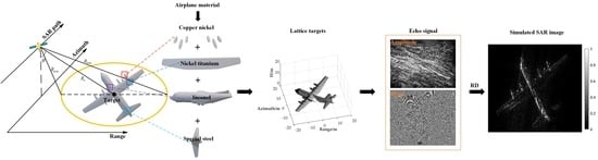
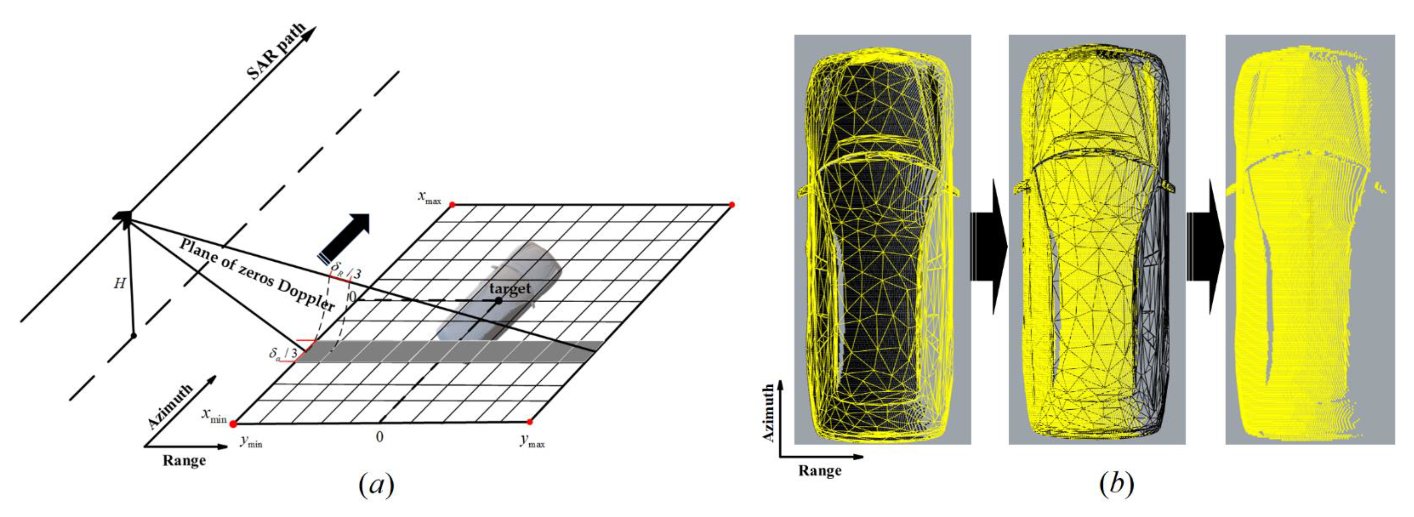
• An SAR effective view algorithm is designed to directly discretize the facets set in the SAR irradiated area into lattice targets. The algorithm adopts the idea of dual-scale subdivision and follows the SAR actual working system mode.
• A novel echo-based SAR image simulation method is proposed to improve the fidelity of simulated SAR images. The method provides a new research idea to combine the ray tracing algorithm and echo time-domain simulation. The method includes multiple scattering and records various kinds of backscatter coefficient for each point target within the synthetic aperture time.
• The proposed method is qualitatively and quantitatively evaluated with real scattering path analysis and structural similarity, respectively.

This paper is organized as follows: Section 2 introduces target model latticing using the SAR effective view algorithm. On the basis of lattice targets, Section 3 introduces echo time-domain simulation and imaging of lattice targets based on the ray tracing algorithm. Section 4 illustrates SAR image simulation tests on several facet target models, providing objective analysis and comparison of experimental results to verify the effectiveness of the proposed method.

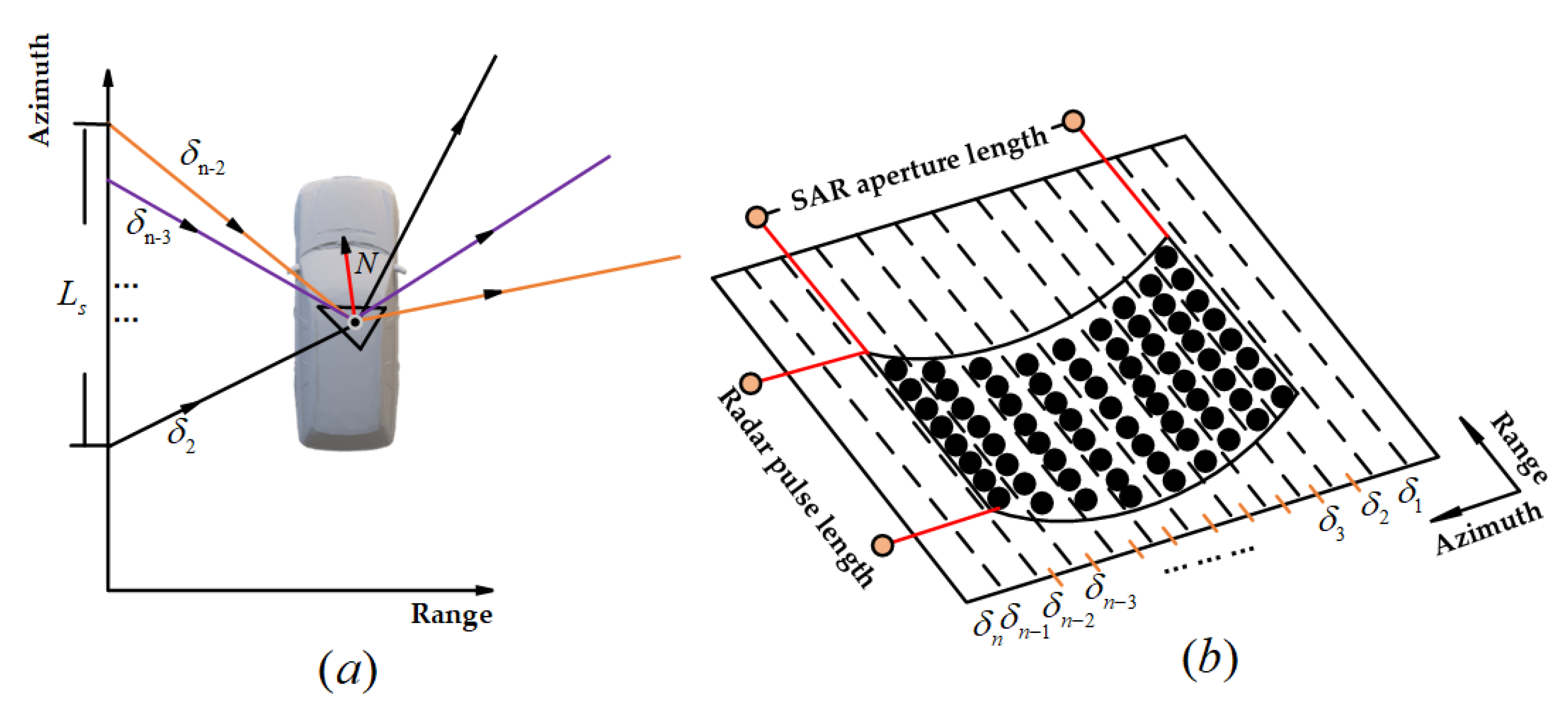
2. Target Model Latticing Using the SAR Effective View Algorithm

The direct processing unit of echo time-domain simulation is a discrete point target. The direct tracking object of the ray tracing algorithm is a discrete electromagnetic wave. Therefore, target discretization is the precondition to combine the ray tracing algorithm and raw echo time-domain simulation.

We mainly use the SAR effective view algorithm to discretize the model facets set in the SAR effective view into lattice targets. The definition of the SAR effective view is mainly based on the beamwidth in the azimuth and range directions. Due to the limitation of the Nyquist sampling law, the sampling interval of lattice targets is less than the resolution of the SAR system. In addition, we can complete the task of eliminating invalid facets in the SAR ineffective view and adopt the idea of dual-scale subdivision of facets to prevent excessive subdivision of facets under the condition of ensuring a clear model texture. We can use the coordinates of lattice targets to provide the incident direction of electromagnetic waves for echo time-domain simulation of lattice targets based on the ray tracing algorithm. In short, target model latticing can provide the basic condition for the combination of the ray tracing algorithm and SAR echo time-domain simulation.

Figure 1 shows the specific flowchart of the SAR effective view algorithm. First, we obtain the incident direction and transmitted position of electromagnetic waves in the SAR effective view by constructing the lattice model. Then, discrete electromagnetic waves in the SAR effective view are simulated. The actual intersection process of SAR transmitted pulses and targets is reproduced. Subsequently, we calculate each intersection point coordinate and record lattice coordinates. Finally, we complete target model latticing.

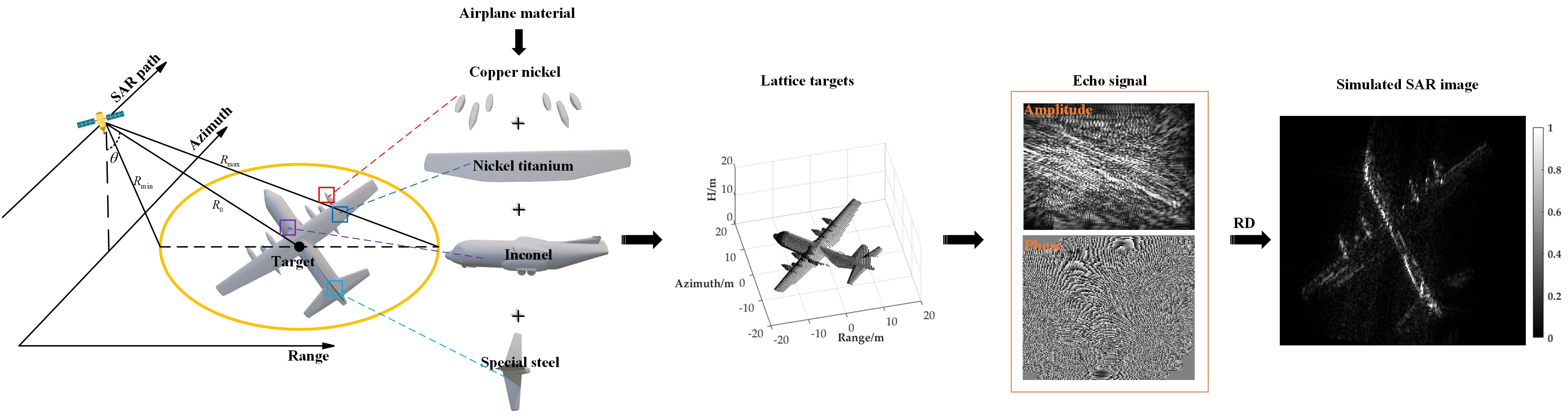
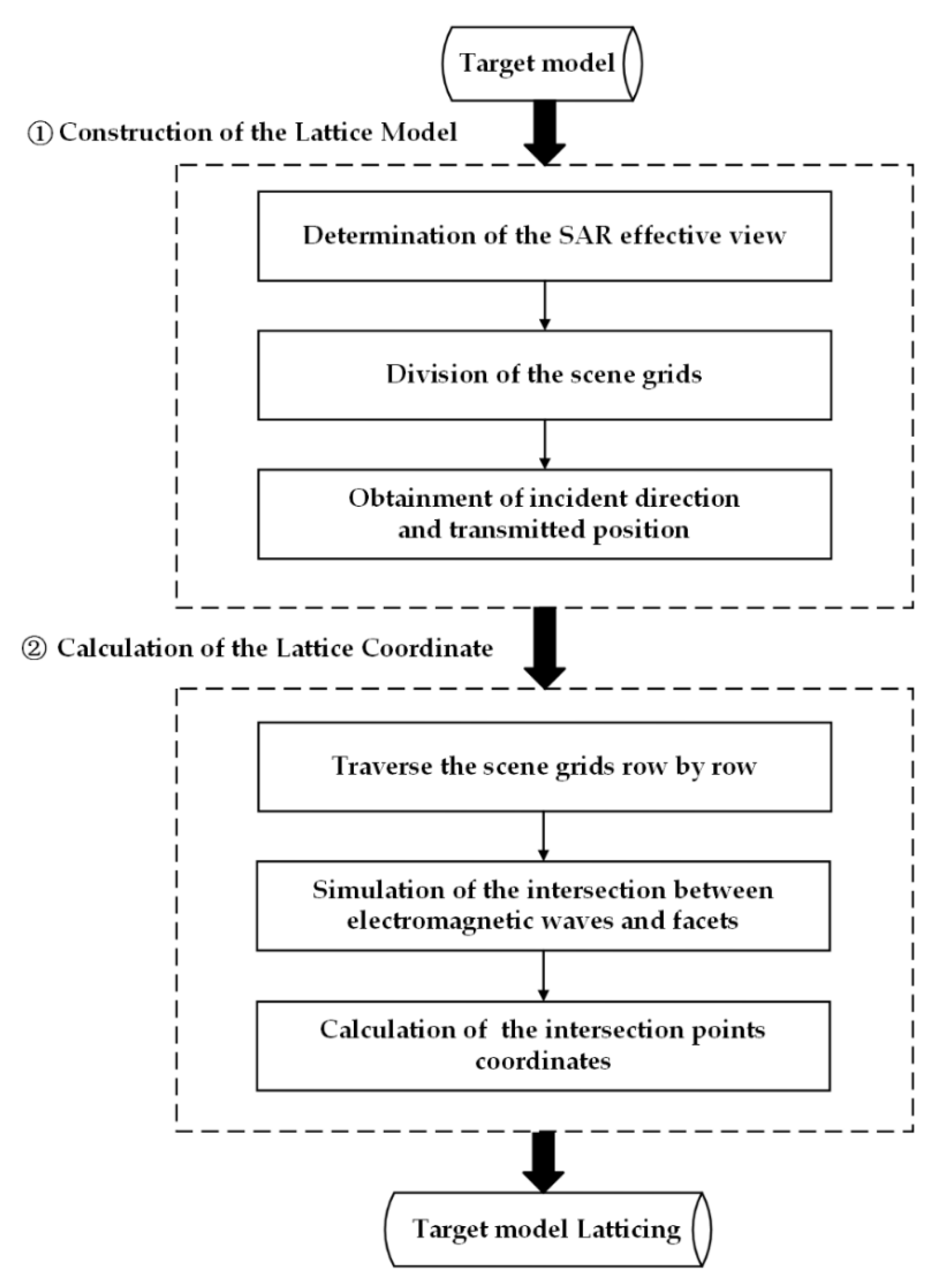
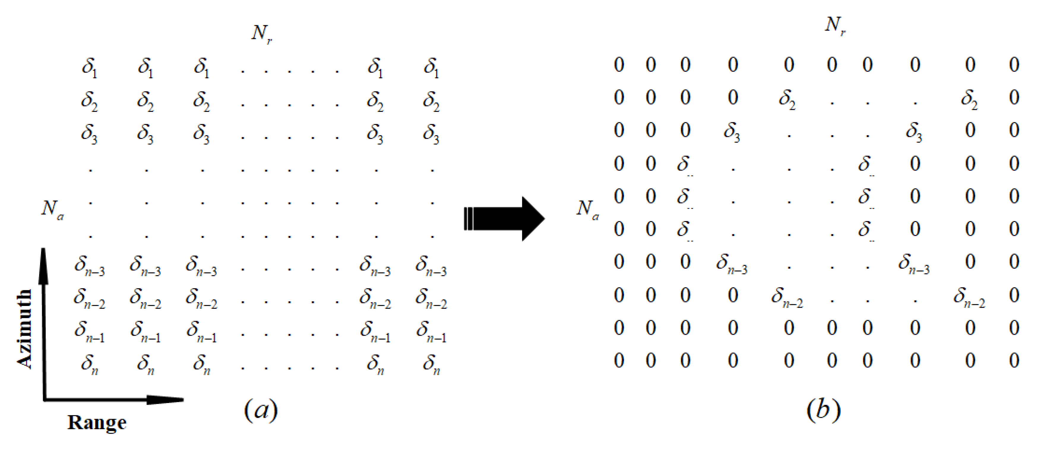
2.1. Construction of the Lattice Model

As shown in Figure 2, we first unify the coordinates of the SAR platform and the target model to determine the SAR effective view. In particular, when the airborne SAR platform and the stop-and-go model are selected, the radiation direction of radar beams are unchanged relative to the flight direction, and the geometric relationship between the platform and the scene is fixed within the azimuth sampling interval. In addition, the platform velocity is designed to be the same as the radar beam scans the scene [33]. The above provides the basic conditions for determining the SAR effective view.

The definition of the SAR effective view is mainly based on the beamwidth in the azimuth and range directions. The radar azimuth beamwidth can be expressed as:

$${\theta }_a=k\lambda /D_a$$

(1)

where ${\theta }_a$ is the radar azimuth beamwidth, $\lambda$ is the wavelength, $D_a$ is the antenna size in the azimuth direction, and $k$ is the scale factor, which is usually set to 0.886.

The radar range beamwidth covers the ground area from the near range to the far range. From the geometric relationship of the lattice model, we can obtain:

$$\left\{\begin{array}{c}{\theta }_{\min }=\arctan ((H*\tan \theta -y_{\min })/H)\\ {\theta }_{\max }=\arctan ((H*\tan \theta +y_{\max })/H)\\ {\theta }_r=[\begin{array}{cc}{\theta }_{\min }& {\theta }_{\max }\end{array}]\end{array}\right.$$

(2)

where ${\theta }_r$ is the radar range beamwidth, ${\theta }_{\min }$ is the minimum incident angle, ${\theta }_{\max }$ is the maximum incident angle, $y_{\min }$ is the scene near range coordinate, $y_{\max }$ is the scene far range coordinate, $\theta$ is the incident angle from the SAR to the scene center, and $H$ is the platform height.

The sampling intervals of azimuth and slant range are set strictly following Nyquist’s sampling law. We refer to the theoretical resolution of the SAR system to set the sampling intervals of azimuth and slant range. In this paper, the sampling intervals are set to one-third of the SAR system resolution. The SAR scene corresponding to the SAR image can be divided into grids by Equation (3), which has M rows along the azimuth direction and N columns in the slant range direction:

$$\left\{\begin{array}{c}M=\frac{x_{\max }-x_{\min }}{{\delta }_a/3}+1\\ N=\frac{y_{\max }-y_{\min }}{{\delta }_R/3}+1\end{array}\right.$$

(3)

where $M$ and $N$ are the number of azimuth rows and range columns, respectively, corresponding to the SAR image. In addition, ${\delta }_a$ and ${\delta }_R$ are the azimuth resolution and slant range resolution, respectively.$x_{\min }$ is the scene minimum coordinate along the azimuth direction, and $x_{\max }$ is the scene maximum coordinate along the azimuth direction.

To improve the efficiency of target latticing, we set each row of the divided grids to be the scanning unit, which is equivalent to using the plane of zeros Doppler to scan the target model, obtaining the coordinates of the intersection of the electromagnetic wave and the scene to be simulated by each row. It is necessary to sequentially determine the transmitted position coordinates and incident direction of each row of electromagnetic waves in the divided grids.

The transmitted position coordinates of the electromagnetic wave of each row along the azimuth direction of the divided grids can be written as:

$$\left\{\begin{array}{c}{x}_i=i*{\delta }_a/3-x_{\min }\hfill \\ S=\left[\begin{array}{cc}{x}_i,& \begin{array}{cc}-H\ast \tan \theta ,\hfill & H\end{array}\end{array}\right]\hfill \end{array}\right.\begin{array}{cc}& i\le M\end{array}$$

(4)

where $x_i$ represents the coordinates along azimuth transmitted electromagnetic waves and $S$ represents the real-time coordinates of the platform.

The geometric relationship among the incident angle, platform height and sampling interval of each column along the slant range direction can be expressed as:

$$\left\{\begin{array}{c}{\theta }_{k+1}=\arccos (H/\left(H/\cos {\theta }_k+{\delta }_R/3\right)\hfill \\ {\theta }_{k+1}-{\theta }_k\sim {\delta }_R/3\hfill \end{array}\right.$$

(5)

where ${\theta }_{k+1}$ and ${\theta }_k$ are adjacent incident angles and where the interval between adjacent incident angles corresponds to the slant range sampling interval.

Derived from Equation (5), the real-time incident direction of electromagnetic waves in each column of the grids can be obtained as:

$$\left\{\begin{array}{cc}\begin{array}{c}{R}_l=R_{\min }+j\ast {\delta }_R/3\hfill \\ {\theta }_j=\arccos (H/R_l)\hfill \\ \overrightarrow{dir}=\left[\begin{array}{ccc}0,& \sin {\theta }_j,& -\cos {\theta }_j\end{array}\right]\hfill \end{array}& j\le N\hfill \end{array}\right.$$

(6)

where $R_l$ is the slant range from radar to each range cell, which is mainly calculated according to the number of range cells spanned in the Doppler plane of zeros of radar beams. In addition, ${\theta }_j$ is the incident angle of the transmitted electromagnetic wave, and $\overrightarrow{dir}$ is the incident direction of the transmitted electromagnetic wave.

2.2. Calculation of the Lattice Coordinates

We use the lattice model above to obtain the transmitted position of the platform and incident direction of the electromagnetic wave. On this basis, Equation (7) can be used to calculate the coordinates of the intersection point:

$$P=S+t*\overrightarrow{dir}$$

(7)

where $P$ is the coordinate of the intersection point to be obtained, $\overrightarrow{dir}$ is the incident direction of the electromagnetic wave, and $S$ is the transmitted position of the platform. In addition, $t$ is the distance from the transmitted position of the platform to the intersection point, which is the key to obtaining the coordinates of the intersection point, mainly using the principle of collision between the ray and triangular facet. As shown in Figure 3, the collision process between the electromagnetic wave and triangular facet is analyzed in detail.

The triangular facet is located using a plane equation:

$$\left\{\begin{array}{c}Ax+By+Cz+D=0\hfill \\ D=-(Ax+By+Cz)\hfill \end{array}\right.$$

(8)

In Equation (8), the plane normal vector $N$ is expressed as $(A,B,C)$. Substituting the vertex $p_1$ of the triangular facet into Equation (8), we obtain:

$$D=-dot(N,p_1)$$

(9)

The electromagnetic wave starts from the platform position $S$ and travels the distance $t$ in the incident direction $\overrightarrow{dir}$ to strike the point $P$, which can be expressed as:

$$P=S+\overrightarrow{dir}·t$$

(10)

Because point $P$ is on the plane, we substitute $P$ into Equation (9) to obtain:

$$dot(P,N)+D=0$$

(11)

$$\left\{\begin{array}{c}dot(S+\overrightarrow{dir}\ast t,N)+D=0\hfill \\ dot(S,N)+dot(\overrightarrow{dir},N)\ast t+D=0\hfill \end{array}\right.$$

(12)

Through the above transformation Equation (12), the distance from the transmitted position to the intersection point can be given by:

$$\left\{\begin{array}{c}t=-\frac{D+dot(S,N)}{dot(\overrightarrow{dir},N)}\hfill \\ t=\frac{dot(N,p_1)-dot(S,N)}{dot(\overrightarrow{dir},N)}\hfill \end{array}\right.$$

(13)

It cannot yet be determined whether point $P$ lies inside or outside the triangular facet. The additional conditions that need to be added are expressed as:

$$\left\{\begin{array}{c}{c}_1=cross(p_2-p_1,P-p_1)\hfill \\ c_2=cross(p_3-p_2,P-p_2)\hfill \\ c_3=cross(p_1-p_3,P-p_3)\hfill \end{array}\right.$$

(14)

$$\left(\begin{array}{l}dot(c_1,N)>0\\ dot(c_2,N)>0\\ dot(c_3,N)>0\end{array}\right)or\left(\begin{array}{l}dot(c_1,N)<0\\ dot(c_2,N)<0\\ dot(c_3,N)<0\end{array}\right)$$

(15)

When the above additional conditions are met, we can determine that point $P$ is in the triangular facet, and its coordinates are expressed as $P=S+t*\overrightarrow{dir}$.

In short, the SAR effective view algorithm proposed in this paper is consistent with the SAR working principle to obtain scene information. In fact, we calculate the lattice coordinates mainly by making each row of scene grids the scanning unit, as shown in Figure 4a. Specifically, according to the azimuth sampling interval ${\delta }_a/3$ and the range sampling interval ${\delta }_R/3$, the coordinates of intersection points between the Doppler plane of zeros and scene grids are sequentially obtained. Finally, the coordinates of the intersection points are recorded in a list format to complete target model latticing in the SAR effective view.

The dual-scale subdivision idea allows us to obtain lattice targets while maintaining the dimension of original irregular surface facets of target models. We can use large surface facets for planar structures and small surface facets for curved structures. As shown in Figure 4b, the invalid facets in the occlusion of the SAR view are eliminated to realize the transformation of facets in the SAR effective view to lattice targets. The SAR effective view algorithm makes the occluded facets as shadow areas, and these facets are temporarily eliminated without changes in the facets’ dimensions. The whole target model with original irregular surface facets is taken into the echo simulation experiment to prevent excessive subdivision of facets. The surface facets of irradiated and shadowed areas are still coherent and not independent of each other. Simulating the multiple scattering of electromagnetic waves can effectively preserve the quantitative impact of facets with different properties in the whole areas on the energy decay of multiple scattering of electromagnetic waves. In summary, we adopt dual-scale subdivision, which can prevent excessive subdivision of facets and improve the intersection speed of electromagnetic waves and facets, and reproduce the coherence impact of irradiated and shadowed areas on the energy decay of multiple scattering of electromagnetic waves.

The SAR effective view algorithm is used to discretize the facets set in the SAR effective view into lattice targets. The discretization of the target is the precondition to combine the ray tracing algorithm and the echo time-domain simulation. After the coordinates of lattice targets are obtained, we can combine the transmitted position of the platform to provide the incident direction of the electromagnetic wave for the SAR echo simulation. Finally, the discrete electromagnetic waves are simulated and generated in the SAR effective view. Then, the echo time-domain simulation of lattice targets can be carried out.

3. Echo Time-Domain Simulation and Imaging of Lattice Targets Based on Ray Tracing Algorithm

The echo time-domain simulation mainly includes magnitude and phase. In terms of magnitude simulation, the standard illumination model is comprehensively improved based on the characteristics of the SAR actual work. The material property parameters of the surface facets participate together in the simulation of the backscatter energy, so as to obtain the magnitude of the backscatter coefficient. In terms of phase simulation, the ray tracing algorithm is mainly used in the time-domain to trace the multiple scattering paths of the electromagnetic wave. Then, multiple scattering paths and the coordinates of each intersection point of the sub-scattering can be successively obtained so as to accurately record the distance of each path. Finally, we can precisely record the phase corresponding to the magnitude of the backscatter coefficient.

The specific process of conducting echo time-domain simulation and imaging of lattice targets based on the ray tracing algorithm is shown in Figure 5. On the basis of the lattice targets, we first select a reasonable illumination model. The corresponding improvements are made according to the geometric and scattering properties of the interaction between the radar and the target. Then, we set the parameters of the echo time domain simulation and combine these with the improved illumination model to obtain the multiple backscatter fields of the target. In the SAR time-domain simulation process, the echo signal of the point target is used as the basic unit of the echo signal of the lattice targets. In addition, the propagation of discrete electromagnetic waves corresponding to each point target is also independent, so we use ray tracing algorithm to trace the multiple scattering paths of each discrete electromagnetic wave. Finally, the operation of vector superposition is performed on the echo signal of all lattice targets to obtain the echo signal of the whole target including multiple scattering. The RD imaging algorithm is used to process the echo signal. Finally, we obtain the simulated SAR image.

3.1. Improvement of the Illumination Model

Light waves and microwaves are both types of electromagnetic waves, and the transmission principle is the same. The classical ray tracing algorithm is an illumination model that solves the algorithm for the intensity of light waves. Considering that the propagation characteristics of high-frequency electromagnetic waves are similar to those of light waves, the classical ray tracing algorithm can be used to calculate the electromagnetic scattering characteristics. Therefore, the illumination model in the field of computer graphics can be applied to the interaction process between the microwave and the target. Because SAR is an active microwave imaging sensor, we need to fully follow the actual interaction between the radar and the target mentioned above. Furthermore, the illumination model needs to be improved locally before we perform echo time-domain simulation based on ray tracing.

To effectively combine the ray tracing algorithm and echo time-domain simulation, we need to make some improvements to the standard illumination model. It is worth noting that we use the SAR effective view algorithm proposed in Section 2 to obtain lattice targets, which can pre-determine the incident direction of the simulated electromagnetic waves. Thus, the “forward-ray tracing” algorithm can be used to improve the illumination model, which improves the stability of the improved model. The specific improvements are as follows:

1)

The “stop-and-go” SAR signal mode is adopted.

2)

The transmitting and receiving energy are located at the same position.

3)

The actively transmitted microwave is the only energy source.

4)

Multiple backscatter fields include the magnitude and phase.

5)

The distance decay factor is added. The backscatter energy is inversely proportional to the 4th power of the propagation distance.

The standard illumination model is a local illumination model, which only involves the case where the facets are directly illuminated by the light source, and does not systematically represent multiple reflections between facets. Therefore, we only use Equation (16) to describe the generation process of the standard illumination model to be improved in detail, and then make reasonable improvements according to the actual working mode of SAR. In the field of computer graphics, the total energy involved in image rendering is usually divided into four mutually exclusive parts: diffuse reflection energy, specular reflection energy, ambient light energy, and self-illumination energy. Among these, diffuse reflection and specular reflection are dependent on specific light sources, ambient light is generally global, and self-illumination is generally related only to the material type [34,35]. Specifically, considering the case of multiple light sources, we can use Equation (16) to superimpose the four mutually exclusive energy as the total recorded energy:

$$\left\{\begin{array}{c}{I}_d={\displaystyle \sum _i^n{K}_d\ast I_{in}^i\ast \max (0,\overrightarrow{v}·\overrightarrow{N})}\hfill \\ I_s={\displaystyle \sum _i^n{K}_f\ast I_{in}^i\ast \max {(0,\overrightarrow{v}·\overrightarrow{r})}^{K_S}}\hfill \\ I_{tol}=I_{amb}+I_d+I_s+I_{emi}\hfill \end{array}\right.$$

(16)

where $I_i$ is the incident energy of the light source, the number of light sources is equal to $n$, $I_{in}$ is the incident initial energy, $I_d$ is the diffuse reflection energy, $I_s$ is the specular reflection energy, $I_{amb}$ is the ambient light energy, $I_{emi}$ is the self-illumination energy, $I_{tol}$ is the total energy recorded, $\overrightarrow{v}$ is the vector of the incident direction, $\overrightarrow{r}$ is the vector of the reflection direction, $\overrightarrow{N}$ is the normal vector of the facet, and the $\max \left(·\right)$ function prevents the whole calculation from being negative. $K_d$ is the diffuse reflection coefficient, $K_f$ is the specular reflection coefficient, $K_s$ is the specular reflection index, and $K_{los}$ is the energy decay coefficient.

Because the actual material of the target is opaque, with certain roughness and gloss properties, we do not consider transmission and refraction but only the reflection and absorption between electromagnetic waves and the target surface. Combining the roughness and metallic gloss of the actual target surface material, we divide the actual interaction types between the incident electromagnetic wave and the target surface into diffuse reflection, specular reflection, and energy absorption. Due to the side-looking working mode of the SAR, when the receiving direction of the platform sensor is close to the specular direction of the target, the radar will receive the specular reflected energy. The parameters of the improved illumination model mainly include the initial incident energy, propagation distance, real-time incident angle, and material properties. Backscatter energy mainly includes diffuse reflection energy and the energy close to the direction of specular reflection. In addition, forward-scatter energy mainly includes the energy transmitted in the direction of specular reflection. The direct manifestation of absorbed energy is energy decay.

According to the actual physical properties of the target, the material property parameters mainly include the diffuse reflection coefficient, specular reflection coefficient, specular reflection index, and energy decay coefficient. Setting the distance decay factor is mainly based on the quantitative relationship in which the backscattered energy is inversely proportional to the 4th power of the propagation distance. The energy decay coefficient covers other forms of energy loss related to the permittivity, such as latent layer absorption and thermal radiation at the target surface. The actual physical properties of the target microfacet include roughness and metallic gloss. Finally, we use Equations (17) and (18) to represent the improved illumination model that records multiple backscatter fields, including the multiple backscatter magnitude and the corresponding phase:

$$\left\{\begin{array}{c}{I}_{in(k)}=I_{in1}\ast {(1-K_{los})}^{k-1}\hfill \\ I_{s(k)}=K_d\ast I_{\mathrm{in}\left(\mathrm{k}\right)}\ast \max (0,\overrightarrow{v}·\overrightarrow{N})+K_f\ast I_{in(k)}\max {(0,\overrightarrow{v^{″}}·\overrightarrow{r})}^{K_S}\hfill \\ I_{s(1)}+I_{s(2)}+\dots +I_{s(k)}<I_{in1}\hfill \end{array}\right.\begin{array}{cc}& (I_{in(k)}<I_{end})\end{array}$$

(17)

$$\left\{\begin{array}{c}\left|\delta (\tau ,\eta ,k)\right|=4\pi R_k{\left(\eta \right)}^2\times \left[\frac{1}{R_k{\left(\eta \right)}^4}\right]\times \frac{I_{s(k)}}{I_{\mathrm{in}1}}=\frac{4\pi }{R_k{\left(\eta \right)}^2}\times \frac{I_{s(k)}}{I_{\mathrm{in}1}}\hfill \\ R_k\left(\eta \right)=\left({R^{\prime }}_1+{R^{\prime }}_2+\dots +{R^{\prime }}_k+R^{″}\right)/2\hfill \\ \overrightarrow{\delta }(\tau ,\eta ,k)={\displaystyle \sum _{k=1}^M\left|\delta (\tau ,\eta ,k)\right|\left[\exp \left\{-j\frac{4\pi f_0{R}_k(\eta )}{c}\right\}\exp \left\{j\pi K_r{\left(\tau -\frac{2R_k(\eta )}{c}\right)}^2\right\}\right]}\hfill \end{array}\right.$$

(18)

where $I_{in\left(k\right)}$ represents the forward-transmitted energy after $k$ times of scattering. $K_{los}$ is the energy decay coefficient, which varies with different facets materials. After each scattering, forward-transmitted energy attenuates according to $K_{los}$, and the energy contribution to the overall scattered field gradually becomes smaller until the energy threshold $I_{end}$ will discard it. $I_{s(k)}$ is the $k$-th backscatter energy of the point target. The sum of the multiple backscatter energy received by the sensor must be less than the initial incident energy $I_{in1}$ of the discrete electromagnetic wave. $f_0$ is the radar carrier frequency and $K_r$ is the range frequency modulation (FM) rate. $\overrightarrow{v^{″}}$ is the vector of the receive direction from the $k$-th intersection point on the target to the sensor’s instantaneous position. $R_k\left(\eta \right)$ is the instantaneous slant range of the $k$-th scattering, which is equivalent to half the sum of the slant range from the sensor’s instantaneous position to the $k$-th intersection point on the target. $R^{\prime }$ is the distance between two adjacent scattering intersections of the electromagnetic wave. $R^{″}$ is the distance from the $k$-th intersection point on the target to the sensor’s instantaneous position. $\left|\delta (\tau ,\eta ,k)\right|$ is the magnitude in the $k$-th backscatter coefficient of the point target. $\overrightarrow{\delta }(\tau ,\eta ,k)$ includes all backscatter fields of the point target. In the specific test, the beam sidelobes effect needs to be limited by envelopes. $\frac{1}{R_k{\left(\eta \right)}^4}$ is the distance decay factor. The parameters relating to multiple scattering are only predefined, with detailed reference to Section 3.3.

After the above specific improvements to the standard illumination model, the improved illumination model fully considers the facet materials’ properties and multiple backscatter fields. It also provides the basic condition for the effective combination of the ray tracing algorithm and SAR echo simulation model.

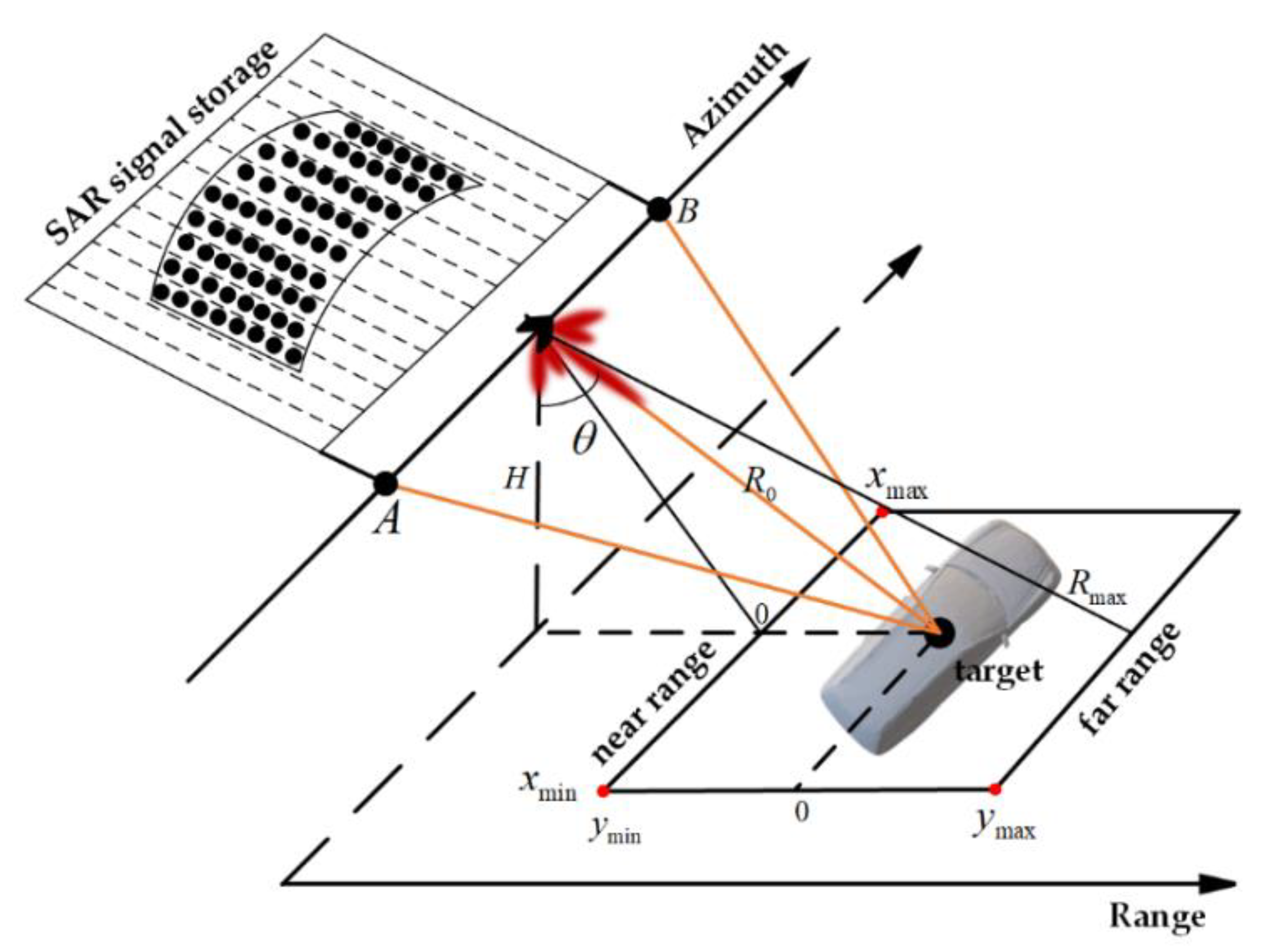
3.2. Setting of the Echo Time-Domain Simulation Model

SAR echo time-domain simulation regards the echo signal as a two-dimensional signal, as shown in Figure 6. Assuming that the azimuth beamwidth is finite, we take the point target P as an example. When the sensor moves to point A, target point P enters the irradiation area of the radar beams. Then, the sensor transmits pulses in sequence along the azimuth direction according to the sampling interval of the pulses. Furthermore, the corresponding echo signal is continuously recorded into the SAR signal storage row by row.

In fact, the radar azimuth beamwidth is infinite, and the echo energy of each point target received by the radar beam sidelobes outside the synthetic aperture time is also recorded in the SAR signal storage. Therefore, the azimuth signal envelope is usually set to limit the radar azimuth beamwidth. We can use Equation (1) to calculate the radar azimuth beamwidth ${\theta }_{az}$ and then combine the slant range $R_0$ from the target to the scene center to obtain the synthetic aperture length $L_s={\theta }_{az}\ast R_0$.

The time axis along the azimuth is determined by parameters such as the scene azimuth length, platform velocity, and pulse frequency. The start and end positions of the scene in the azimuth direction have full synthetic aperture illumination time. The time axis in the azimuth direction can be expressed as:

$$\left\{\begin{array}{c}{t}_a=\left[(x_{\min }-\frac{L_s}{2})/V_r:(x_{\max }+\frac{L_s}{2})/V_r\right]\hfill \\ at=1/PRF\hfill \\ l_a=V_r\ast at\hfill \end{array}\right.$$

(19)

where $t_a$ is the time axis in the azimuth direction, $x_{\min }$ is the scene minimum coordinate in the azimuth direction, $x_{\max }$ is the scene maximum coordinate in the azimuth direction, and $V_r$ is the platform velocity. $PRF$ is the pulse frequency, $at$ is the azimuth time interval, and $l_a$ is the azimuth sampling interval, which is less than the SAR azimuth theoretical resolution.

The time axis in the range direction is determined by parameters such as the scene range length, platform height, incident angle, pulse width, and pulse sampling frequency. The time axis in the range direction can be given by:

$$\left\{\begin{array}{c}{Y}_c=H*\tan \theta \hfill \\ R_{\min }=\sqrt{{\left(Y_c+y_{\min }\right)}^2}+H^2\hfill \\ R_{\max }=\sqrt{{\left(Y_c+y_{\max }\right)}^2}+H^2\hfill \\ t_r=[2*R_{\min }/c:2*R_{\max }/c+T_r]\hfill \\ rt=1/F_r\hfill \\ l_r=c\ast rt/2\hfill \end{array}\right.$$

(20)

where $t_r$ is the time axis in the range direction, $R_{\min }$ is the shortest slant range, and $R_{\max }$ is the longest slant range. $Y_c$ is the ground range from the SAR to the scene center, $H$ is the platform height, $c$ is the light velocity, $\theta$ is the incident angle, $y_{\min }$ is the scene near range coordinate, and $y_{\max }$ is the scene far range coordinate. $F_r$ is the pulse sampling frequency, $rt$ is the range time interval, and $l_r$ is the azimuth sampling interval, which is less than the SAR range theoretical resolution. The platform coordinates can be determined by Equations (19) and (20).

$$S=\left[\begin{array}{ccc}{t}_a*V_r& H& -Y_c\end{array}\right]$$

(21)

where $S$ represents the platform coordinates, moving at the time axis $t_a$ in the azimuth direction, and its coordinates are variables. $-Y_{\mathrm{c}}$ is the ground range coordinate of the platform, and $H$ is the platform height, which are both fixed values.

Suppose the radar transmits the linear FM signal with rectangular envelope:

$$\left\{\begin{array}{c}\mathrm{s}\left(\tau \right)=\mathrm{re}ct\left(\frac{\tau }{T_r}\right)\exp \left\{j2\pi f_0\tau +j\pi K_r{\tau }^2\right\}\hfill \\ Bw=K_r\ast T_r\hfill \end{array}\right.$$

(22)

where $T_r$ is the pulse duration, usually lasting approximately a few microseconds, $K_r$ is the range frequency modulation (FM) rate, and $Bw$ is the signal bandwidth, which refers to the frequency range occupied by the main pulse energy. In addition, $f_0$ is the radar carrier frequency, and $rect(·)$ represents the range signal envelope, which is an approximately rectangular window.

$$\left\{\begin{array}{l}\theta \left(\tau \right)=2\pi f_0\tau +\pi K_r{\tau }^2\\ f\left(\tau \right)=\frac{1}{2\pi }\frac{d\theta \left(\tau \right)}{d\tau }=f_0+K_r\tau \\ R\left(\eta \right)=\sqrt{R_0^2+V_r^2{\eta }^2}\approx R_0+\frac{V_r{\eta }^2}{2R_0}\end{array}\right.$$

(23)

where $R\left(\eta \right)$ is the instantaneous slant range from the SAR to the point target. The real-time movement of the platform also provides the basis for generating the Doppler frequency history. Here, $\theta \left(\tau \right)$ is the instantaneous phase, and $f\left(\tau \right)$ is the instantaneous frequency. The echo signal received by the radar can be expressed as:

$$\begin{array}{c}{s}_r(\tau ,\eta )=rect(\frac{\tau -2R\left(\eta \right)/c}{T_r})\hfill \\ \hspace{1em}\hspace{1em}\hspace{1em}\hspace{1em}\hspace{1em}\times \exp \left\{j(2\pi f_0(\tau -2R\left(\eta \right)/c)+j\pi K_r{(\tau -2R\left(\eta \right)/c)}^2\right\}\hfill \end{array}$$

(24)

The response signal of the point target after demodulation can be given by:

$$\begin{array}{c}{s}_o\left(\tau ,\eta \right)=w_r\left[\tau -2R\left(\eta \right)/c\right]w_a\left(\eta -{\eta }_c\right)\hfill \\ \hspace{1em}\hspace{1em}\hspace{1em}\hspace{1em}\hspace{1em}\times \exp \left\{-j\frac{4\pi f_{0}R(\eta )}{c}\right\}\exp \left\{j\pi K_r{\left(\tau -\frac{2R(\eta )}{c}\right)}^2\right\}\hfill \end{array}$$

(25)

where $w_r\left(\tau \right)$ and $w_a\left(\eta \right)$ are the range envelope and azimuth envelope, respectively, which can guarantee the coherence of the signal and can be given by:

$$\left\{\begin{array}{c}{w}_a\left(\eta \right)=bool\left[\left|t_a\ast v_a-P_{az}\right|\le L_a/2\right]\hfill \\ w_r\left(\tau \right)=bool\left[\left|t_r-2*R_n/c\right|\le T_r/2\right]\hfill \end{array}\right.$$

(26)

where $P_{az}$ is the azimuth coordinate of the point target, and where $bool$ returns 1 if the condition is satisfied and 0 otherwise.

The observation process of the SAR system to target is equivalent to the two-dimensional convolution process of the backscatter coefficient and the SAR impulse response signal, which can be expressed as:

$$\left\{\begin{array}{c}Echo={\displaystyle \sum _{i=1}^N}\left[{\displaystyle \sum _{k=1}^M}\left|{\delta }_i(\tau ,\eta ,k)\right|\left(\begin{array}{c}{w}_r\left[\tau -2R_k\left(\eta \right)/c\right]w_a\left(\eta -{\eta }_c\right)\hfill \\ \begin{array}{ccc}& & \begin{array}{ccc}& & \hspace{1em}\hspace{1em}\times exp\left\{-j\frac{4\pi f_0{R}_k\left(\eta \right)}{c}\right\}exp\left\{j\pi K_r{\left(\tau -\frac{2R_k\left(\eta \right)}{c}\right)}^2\right\}\end{array}\end{array}\hfill \end{array}\right)\right]\hfill \\ \left[Echo\right]=〈a+bi〉\hfill \\ \left|{\delta }_i(\tau ,\eta ,k)\right|=\frac{4\pi }{R_k{\left(\eta \right)}^2}\times \frac{I_{s\left(k\right)}}{I_{\mathrm{in}1}}\hfill \\ R_k\left(\eta \right)=\left({R^{\prime }}_1+{R^{\prime }}_2+\dots +{R^{\prime }}_k+R^{″}\right)/2\hfill \end{array}\right.$$

(27)

where $Echo$ is the echo signal of $N$ lattice targets, the recording format of each element of the $Echo$ is $a+bi$. The magnitude of the backscatter coefficient is multiplied by the cosine of the corresponding phase as the real part $a$. The magnitude of the backscatter coefficient is multiplied by the sine of the corresponding phase as the imaginary part $bi$. $w_r\left(\tau \right)$ and $w_a\left(\eta \right)$ are the range envelope and azimuth envelope, respectively. $\exp \left\{-j\frac{4\pi f_0{R}_k(\eta )}{c}\right\}$ is the Doppler phase, which is used for azimuth compression, $\exp \left\{j\pi K_r{\left(\tau -\frac{2R_k(\eta )}{c}\right)}^2\right\}$ is the phase delay of the transmitted signal, which can perform range compression. Echo time-domain simulation can ensure the accuracy of the corresponding phase delay of lattice targets.

3.3. Calculation of the Backscatter Field

The echo signal of the point target is used as the basic unit of the whole echo signal of target. Therefore, we first use ray tracing algorithm to assist each point target to perform echo time-domain simulation, which can obtain multiple backscatter fields for each point target, including magnitude and phase. Then, we perform vector superposition of the multiple backscatter fields of each point target to generate the echo matrix of each point target. SAR echo signal simulation adopts the “stop-and-go” model. According to the specific process of conducting echo time-domain simulation, we take the point target as an example. The number of discrete electromagnetic waves is equal to the number of azimuth sampling points. The multiple backscatter fields of all discrete electromagnetic waves are sequentially calculated, including the magnitude and phase of the corresponding backscatter fields.

The number of azimuth sampling points is determined by the scene azimuth length, platform velocity, and pulse frequency, and can be given by:

$$N_a=(x_{\max }-x_{\min }+L_s)/V_r*PRF$$

(28)

where $N_a$ is the number of azimuth sampling points, $x_{\min }$ is the scene minimum coordinate in the azimuth direction, $x_{\max }$ is the scene maximum coordinate in the azimuth direction, $L_s$ is the synthetic aperture length, $V_r$ is the platform velocity, and $PRF$ is the pulse frequency. When setting $PRF$, it should be considered that the azimuth sampling interval is less than the theoretical SAR azimuth resolution. In this paper, the azimuth resolution is 3 and 1 m, and the corresponding azimuth sampling intervals are set to 1 and 0.3 m, respectively.

The number of range sampling points was determined by the slant range, platform height, pulse width, and pulse sampling frequency, and can be expressed as:

$$N_r=\left(2*\left(R_{\max }-R_{\min }\right)/c+T_r\right)*F_r$$

(29)

where $N_r$ is the number of range sampling points, $R_{\min }$ is the shortest slant range, $R_{\max }$ is the longest slant range, $T_r$ is the pulse width, and $F_r$ is the pulse sampling frequency. When setting $F_r$, it should be considered that the range sampling interval is less than the theoretical SAR range resolution. In this paper, the range resolution is 3 and 1 m, the range sampling interval is set to 2 and 0.7 m, and $c$ is the speed of light.

When the platform moves sequentially according to the azimuth sampling interval, the electromagnetic wave is transmitted, and the echo signal is received at the same position. In addition, the number of discrete electromagnetic waves for the point target is equal to the number of azimuth sampling points, and the simulated transmitted of electromagnetic waves can be represented as:

$$\left\{\begin{array}{c}{\overrightarrow{E}}_{dir}=normal(P-S)\hfill \\ Ray=\left[S,{\overrightarrow{E}}_{dir}\right]\hfill \end{array}\right.$$

(30)

where ${\overrightarrow{E}}_{dir}$ is the incident direction of the electromagnetic wave, $Ray$ is the incident electromagnetic wave, and $P$ represents the coordinates of the lattice targets. $S$ represents the platform coordinates, which can be determined by the azimuth discrete time axis, the platform velocity, and platform range coordinates, as shown in Equation (21) for detail. In addition, $normal\left(·\right)$ represents normalization.

The reflection and propagation of electromagnetic waves satisfy Fresnel’s law of reflection, that is, in the plane where the reflected ray, the incident ray, and the normal vector of the intersection point are located, the reflection angle is equal to the incident angle.

$$\overrightarrow{r}=\overrightarrow{v}-2*\max (0,\overrightarrow{v}·\overrightarrow{N})*\overrightarrow{N}$$

(31)

where $\overrightarrow{r}$ is the direction of the transmitted energy for forward ray tracking after each scattering. $\overrightarrow{v}$ is the vector of the incident direction after each scattering, which is completely different from $\overrightarrow{v^{″}}$ in Equation (17).

The electromagnetic wave energy continues to decay in the process of multiple scattering, and its contribution to the total echo energy after multiple decays is not significant. The energy threshold can be set to limit the number of electromagnetic wave tracking. The remaining energy decay after $k$ times scattering can be expressed as:

$$I_{in(k)}=I_{in1}\ast {(1-K_{los})}^{k-1}\hspace{1em}\hspace{1em}(I_{in(k)}<I_{end})$$

(32)

where $K_{los}$ is the energy decay coefficient, which is a variable in the process of multiple scattering energy calculation, because different parts of the facet model have different material properties. In this paper, the initial value of the reflected electromagnetic wave energy is set to unit 1, the end threshold value $I_{end}$ is 0.1, and the recursion ends when it is lower than the threshold value.

The intersection coordinate and instantaneous slant range of the $k$-th scattering of discrete electromagnetic wave are two key factors to calculate the target multiple backscatter fields. The specific process to obtain the two key factors based on the ray tracing algorithm are as follows:

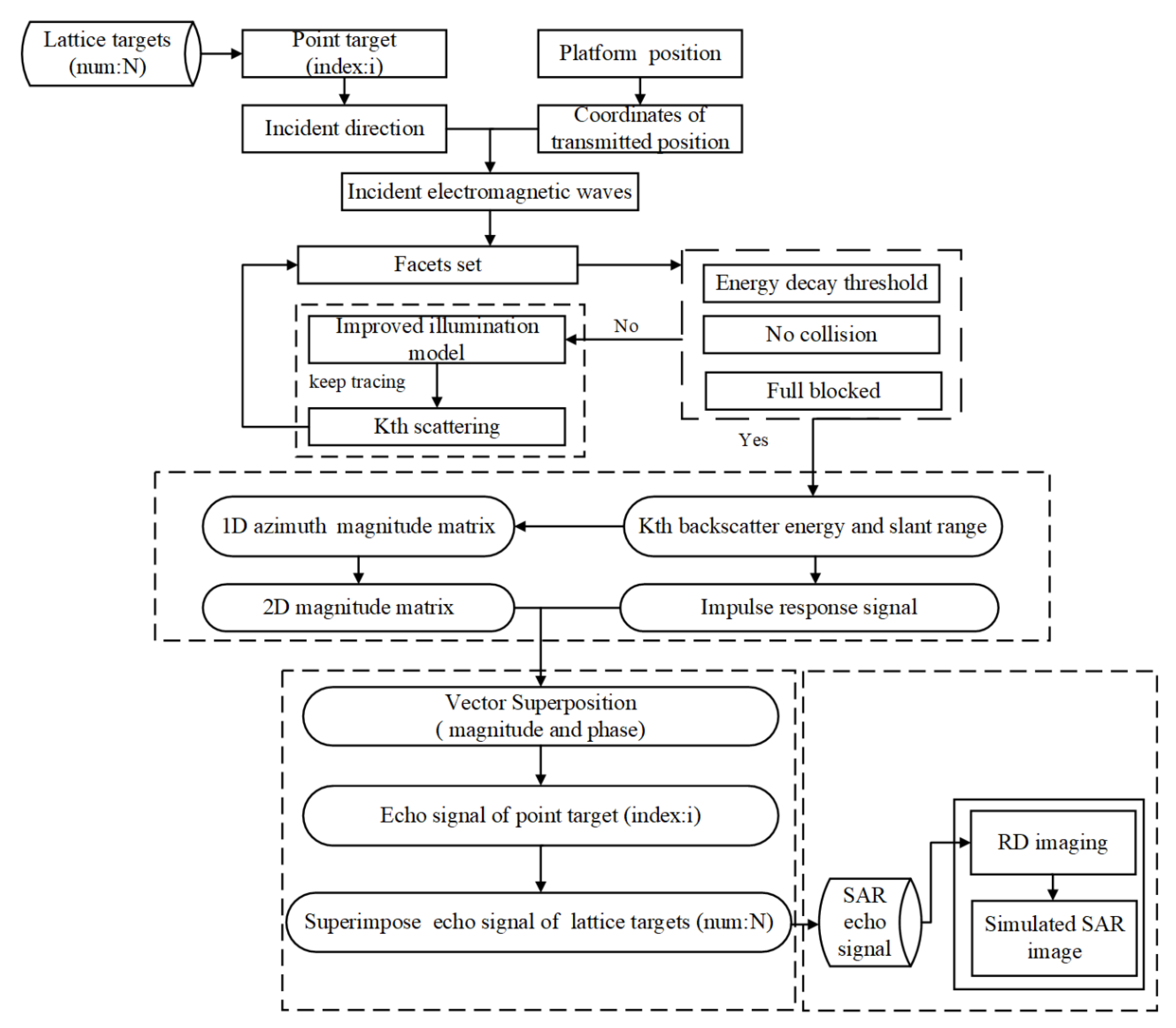
• The sensor instantaneous position can be obtained by Equation (21). The initial incidence direction of the discrete electromagnetic waves can be provided by the lattice targets obtained by using the SAR effective view algorithm, with reference to Equation (30).
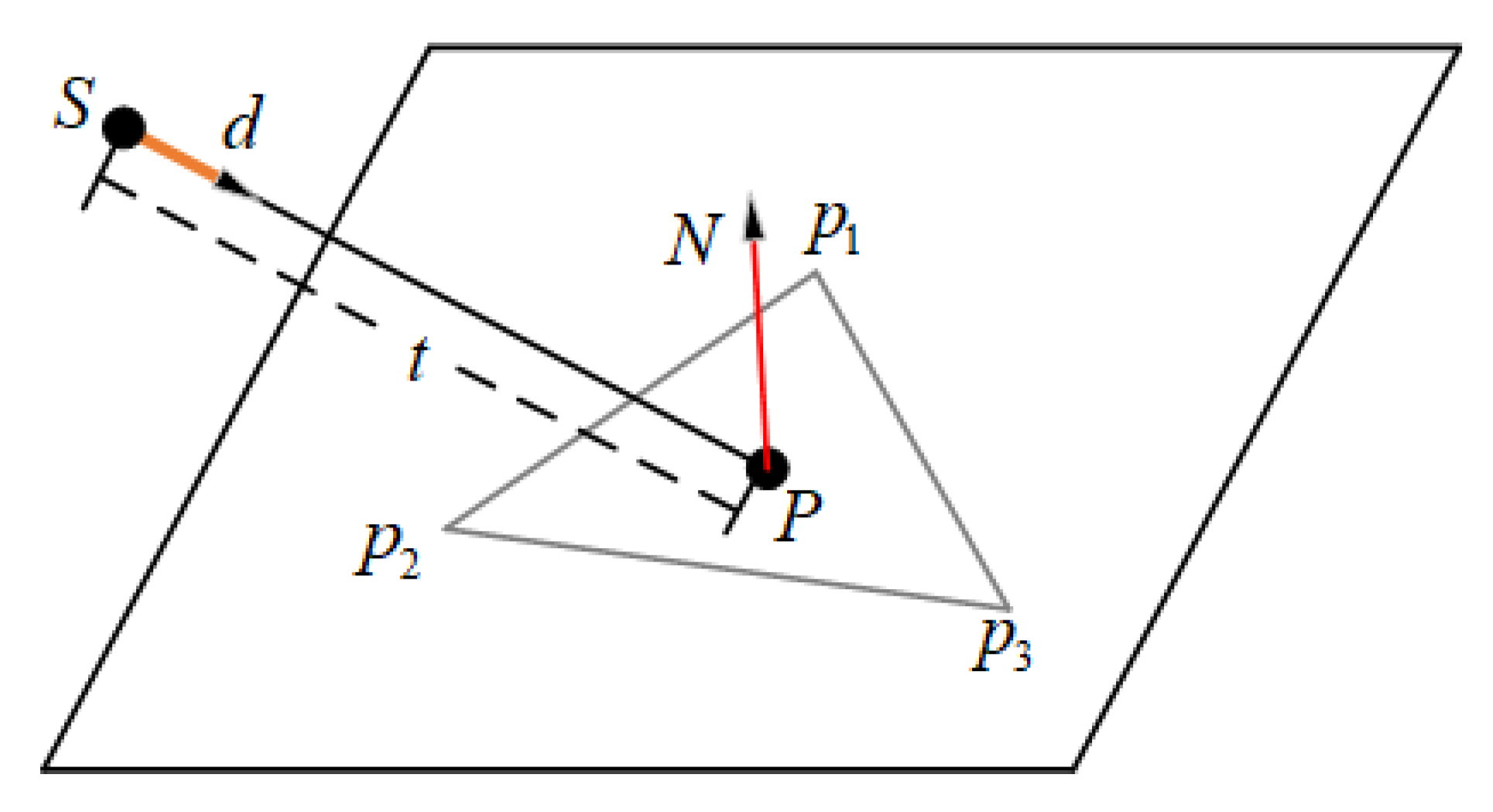
• After simulating the transmitted electromagnetic wave interactions with the target surface, the direction of specular reflection is calculated according to Fresnel’s law of reflection, as shown in Equation (31) for detail.
• The intersection of electromagnetic wave and target surface is used as the new starting point of incidence, and the specular reflection direction is used as the next new incidence direction to alternately complete multiple scattering of electromagnetic waves. The calculation of the single intersection coordinate of electromagnetic wave and target surface can refer to Equations (8)–(15) in detail.
• The termination conditions of multiple scattering are set according to the actual propagation path and energy decay of the electromagnetic wave. As the electromagnetic wave continues to track in the new reflection direction after each scattering, it still needs to traverse all the surface facets to find the location of the nearest collision point. If no collision occurs, the tracking of scattering path will end. After each scattering of the electromagnetic wave, the energy continues to decay, and the tracking of the scattering path will end when the energy decay threshold is met, with reference to Equation (32).
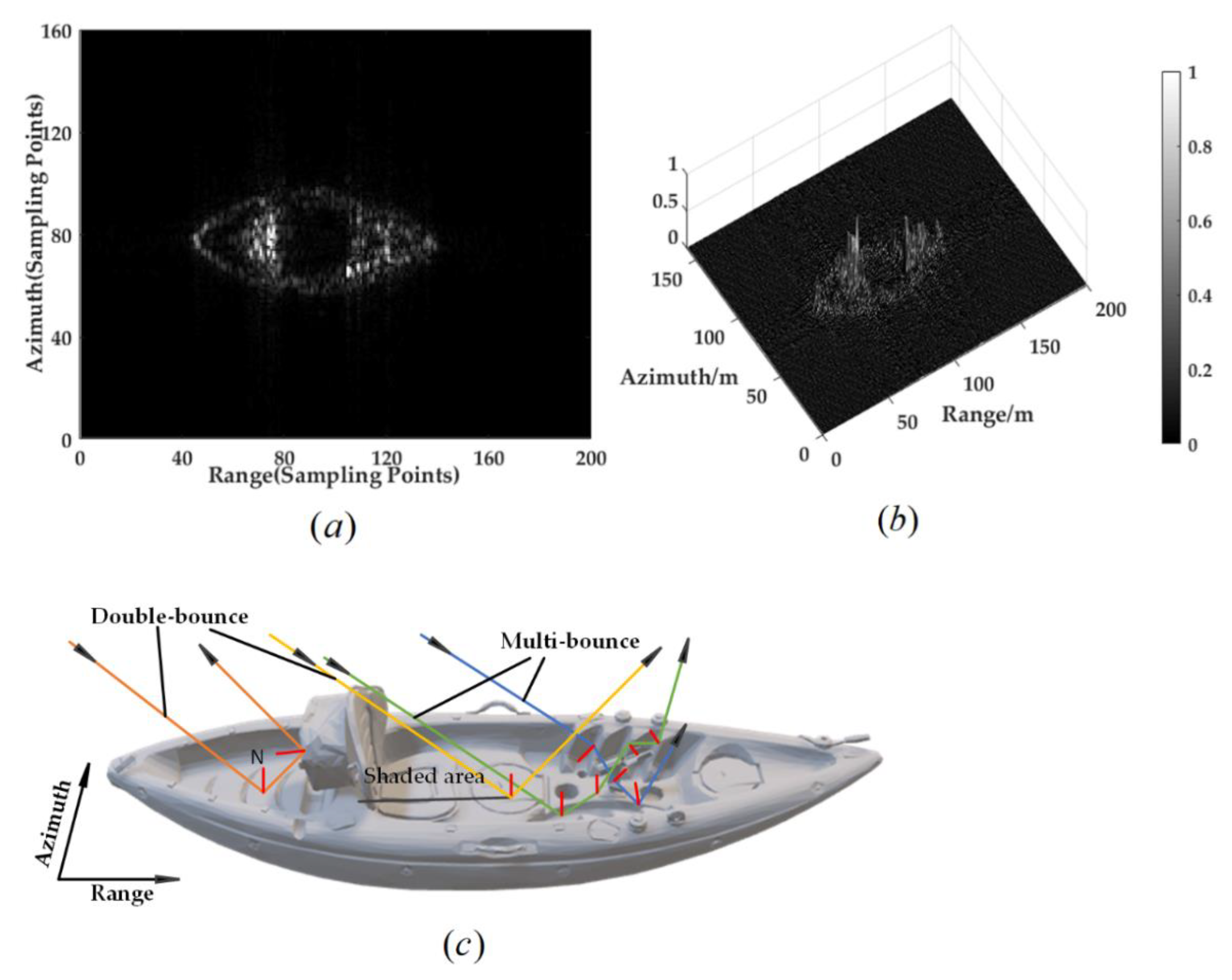
• Due to the complexity of the simulated targets or scenes, the multiple scattering intersections and the sensor location are not guaranteed to be through-view all the time. Therefore, it is necessary to add the through-view condition; that is, if there is a collision point, we transmit a ray from the collision point to the radar platform to see if there is any occlusion, and if so, the intersection of the $k$-th scattering is not visible with the sensor, and the backscattering energy and phase of the point cannot be recorded.
• The intersection coordinate for the $k$-th scattering of electromagnetic wave with the target surface can be obtained in turn using steps 1 to 5, and the instantaneous slant range of the $k$-th scattering can be calculated by Equation (33):

  $$R_k=\left(\begin{array}{c}\sqrt{{\left(S^{\prime }-P_0{}^{\prime }\right)}^2}+\sqrt{{\left(P_0-P_1{}^{\prime }\right)}^2}+\hfill \\ \begin{array}{cccc}& \dots & \dots & +\sqrt{{\left(P_{k-1}{}^{\prime }-P_k{}^{\prime }\right)}^2}+\sqrt{{\left(P_k{}^{\prime }-S^{\prime }\right)}^2}\end{array}\end{array}\right)/2=\left({R^{\prime }}_1+{R^{\prime }}_2+\dots +{R^{\prime }}_k+R^{″}\right)/2$$

  (33)

  where $R_k$ is the instantaneous slant range of the $k$-th scattering, which is equivalent to half the sum of the slant range from the sensor’s instantaneous position to the $k$-th intersection point on the target. $P^{\prime }$ is the intersection coordinate for each scattering. $S^{\prime }$ is sensor’s instantaneous position, as shown in Equation (21) for detail. $R^{″}$ is the distance from the $k$-th intersection coordinate $P_k{}^{\prime }$ on the target to the $S^{\prime }$.

When calculating the intersection coordinates for the k-th scattering of discrete electromagnetic wave with the target surface, the normal vector and index number of the corresponding surface facets are also recorded. Refer to the index number to determine the corresponding material diffuse reflection coefficient $K_d$, specular reflection coefficient $K_f$, specular reflection index $K_s$, energy decay coefficient $K_{los}$, and normal vector $\overrightarrow{N}$ of the surface facet. Backscatter energy includes diffuse energy and energy close to the specular direction. In the process of multiple scattering of each discrete electromagnetic wave and the target surface, electromagnetic waves will intersect with target surface facets with different material property parameters. The propagation path of each discrete electromagnetic wave is traced based on ray tracing. When the selected target models are relatively regular, the termination condition of multiple scattering is mainly no collision point to end the recursion. Assuming that the path tracing of discrete electromagnetic waves is recursive to the greatest extent, the $k$-th backscatter field including magnitude and phase can be expressed as:

$$\left\{\begin{array}{c}{I}_{s(k)}=K_d\ast I_{\mathrm{in}\left(\mathrm{k}\right)}\ast \max (0,\overrightarrow{v}·\overrightarrow{N})+K_f\ast I_{in(k)}\max {(0,\overrightarrow{v^{″}}·\overrightarrow{r})}^{K_S}\hfill \\ \left|\delta (\tau ,\eta ,k)\right|=\frac{4\pi }{R_k{\left(\eta \right)}^2}\times \frac{I_{s(k)}}{I_{\mathrm{in}1}}\hfill \\ Pha(k)=\exp \left\{-j\frac{4\pi f_0{R}_k(\eta )}{c}\right\}\exp \left\{j\pi K_r{\left(\tau -\frac{2R_k(\eta )}{c}\right)}^2\right\}\hfill & (I_{in(k)}<I_{end})\hfill \\ 〈Pha(k)〉=\left[w_r\left(\tau -2R_k\left(\eta \right)/c\right)\times w_a\left(\eta -{\eta }_c\right)\right]\times Pha(k)\hfill \\ R_k\left(\eta \right)=\left(R_1{}^{\prime }+R_2{}^{\prime }+\dots +R_k{}^{\prime }+R^{″}\right)/2\hfill \end{array}\right.$$

(34)

where $I_{s(k)}$ is the $k$-th backscatter energy. $\left|\delta (\tau ,\eta ,k)\right|$ is the magnitude in the $k$-th backscatter coefficient of the point target. $Pha(k)$ is the $k$-th scattering phase, which contains Doppler phase and range phase, respectively. $〈Pha(k)〉$ ensures phase coherence in SAR coherent system. $I_{in(k)}$ after multiple scattering decays to the energy threshold $I_{end}$. $\overrightarrow{v^{″}}$ is the vector of the receive direction from the $k$-th intersection point on the target to the sensor’s instantaneous position, related to receiving specular energy during multiple scattering. $w_r\left(\tau \right)$ and $w_a\left(\eta \right)$ are the range envelope and azimuth envelope, as shown in Equation (26) for detail.

In this paper, the time-varying and space-varying characteristics of target scattering characteristics within the SAR aperture and bandwidth are fully considered. In the time domain, simulated radar pulses are sent and received sequentially in the azimuth direction, and multiple backscatter fields are recorded. Then, we take the calculation of the single scattering field of the point target as an example. In the actual echo simulation tests, we first generate a one-dimensional energy matrix in the azimuth direction, and the matrix size is $N_a\times 1$. As shown in Figure 7, the proposed method fully combines the ray tracing algorithm and the echo time domain simulation model, and reproduces the time-varying and space-varying characteristics of the target backscatter coefficient. It can overcome the limitations of traditional echo simulation models which are mostly based on the assumption of a fixed scattering center.

At the same time, range sampling is carried out, and the number of range sampling points is $N_r$, and a two-dimensional matrix of the single backscatter magnitude of the point target is generated. As shown in Figure 8a, the matrix size is $N_a\times N_r$. The echo signal of the point target can be obtained by vector superposition of the multiple backscatter fields.

Each point target corresponds to $n$ discrete electromagnetic waves transmitted by the platform, which are limited by the azimuth envelope. As shown in Figure 8b, the actual number of effective pulses is equal to the number of transmitted pulses within the synthetic aperture time. Therefore, the two-dimensional $k$-th backscatter field contains less than $n$ kinds of magnitude. Finally, we perform vector superposition of the multiple backscatter fields to obtain the echo signal of the point target.

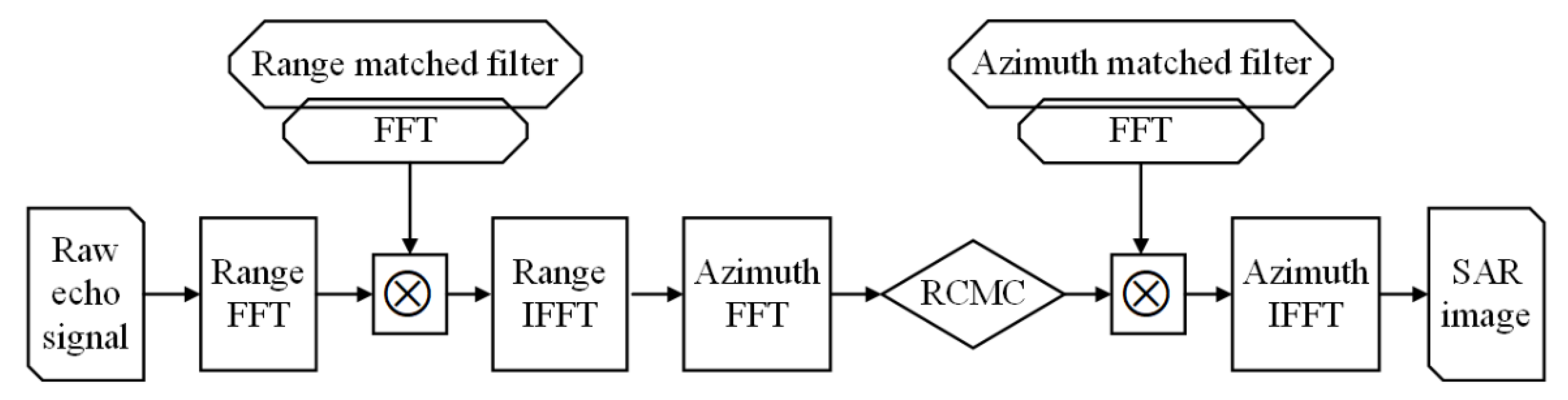
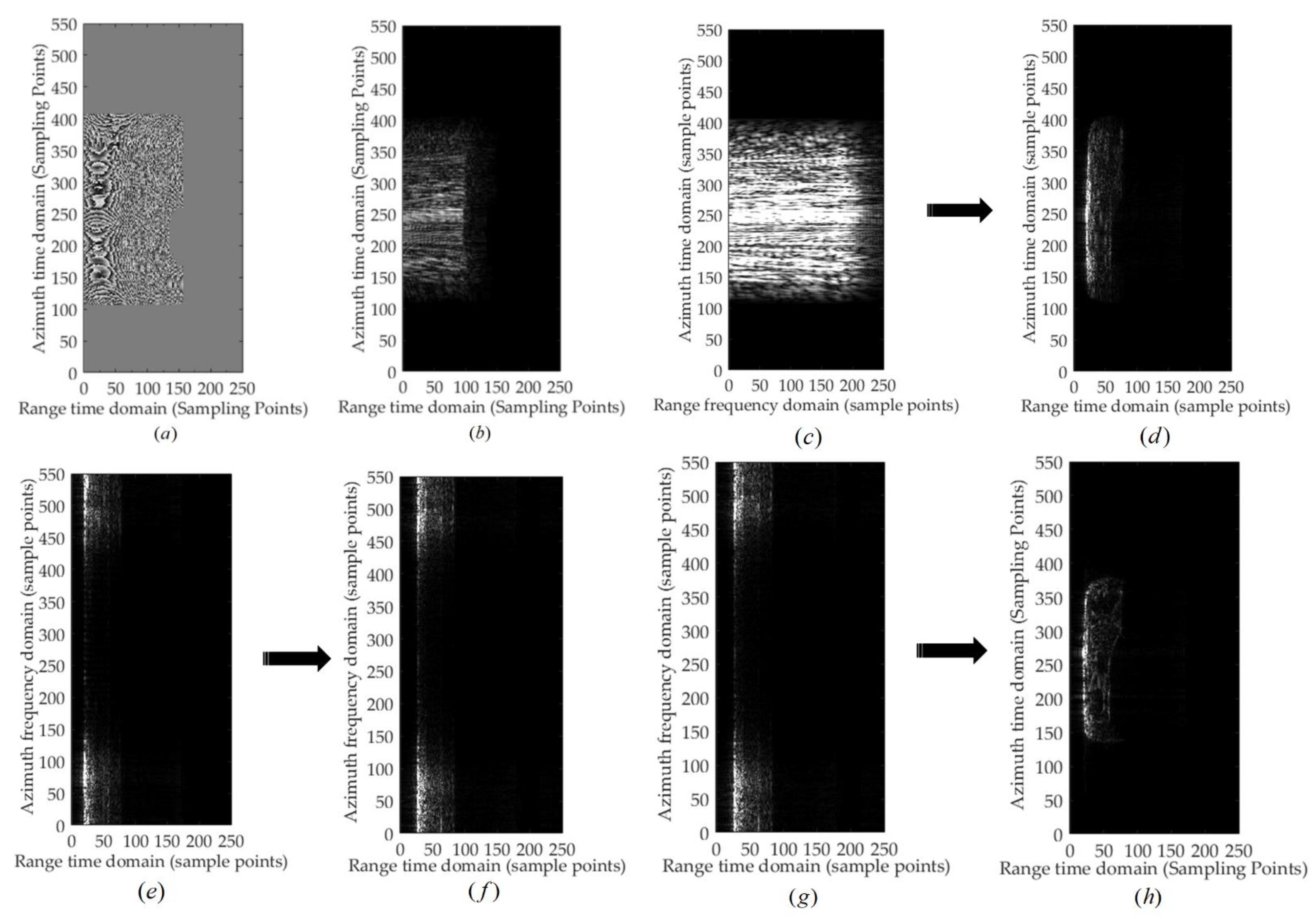
3.4. Generation and Imaging of the Echo Signal

The echo signal of each point target is the basic unit of the whole target echo signal. The operation of vector superposition is performed on the echo signal of all lattice targets to obtain the echo signal of the whole target including multiple scattering. The raw echo signal can be expressed as:

$$\left\{\begin{array}{c}Echo={\displaystyle \sum _{i=1}^{N}Ech{o}_i(\tau ,\eta )}\hfill \\ Ech{o}_i(\tau ,\eta )={\displaystyle \sum _{k=1}^M\left|\delta (\tau ,\eta ,k)\right|\times 〈Pha(k)〉}\hfill \\ \left|\delta (\tau ,\eta ,k)\right|=\frac{4\pi }{R_k{\left(\eta \right)}^2}\times \frac{I_{s(k)}}{I_{\mathrm{in}1}}\hfill \end{array}\right.$$

(35)

where $Echo$ is echo signal of the whole target, which is equal to the vector superposition of the multiple backscatter fields of all lattice targets. $Ech{o}_i$ is the echo signal of the point target, including magnitude and phase. $〈Pha(k)〉$ is the coherence phase, as shown in Equation (34) for detail. $\left|\delta (\tau ,\eta ,k)\right|$ corresponds to the magnitude of the $k$-th backscatter coefficient, as shown in Equations (17) and (18) for detail.

The imaging process of the SAR echo signal can be equivalent to the process of compressing and focusing the echo signal in the azimuth and range directions, as shown in Figure 9. In other words, SAR echo imaging is a two-dimensional deconvolution process that reconstructs the backscatter coefficient of the target.

We take the imaging of car body lattices as an example. The phase and magnitude of the echo signal of lattice targets are shown in Figure 10a,b.

• Range compression: The echo signal before and after range compression are shown in Figure 10c,d, respectively. The principle of stationary phase can be used to implement the range fast Fourier transform (FFT). When the echo signal is in the range frequency domain and the azimuth time domain, range compression can be performed by fast convolution. In particular, a matched filter should be designed to remove the second-order phase. Following the range FFT, the range-matched filter is performed immediately, and then the range compression is completed by using the range inverse Fourier transform (IFFT).
• Azimuth Fourier transform: The echo signal is transformed to the range-Doppler domain through the azimuth FFT, as shown in Figure 10e. Range cell migration correction is usually performed in the range-Doppler domain. In addition, Doppler centroid estimation and most subsequent operations are also performed in this domain.
• Range cell migration correction: As shown in Figure 10f, range cell migration correction is performed in the range-Doppler domain. Usually, in this domain, the trajectories of a group of targets in the same range cell coincide with each other. Mainly through interpolation processing based on the sinc function, the curve trajectory generated by the range cell migration correction can be straightened to be parallel to the azimuth frequency axis.
• Azimuth compression: After the range migration correction, the azimuth focusing of the echo signal can be carried out through the azimuth matched filter. In other words, azimuth compression is mainly achieved through azimuth matched filtering on each range cell, as shown in Figure 10g. Next, the echo signal is transformed to the 2D time domain through IFFT, and the result is the compressed complex image, as shown in Figure 10h.

4. Discussion of Simulation Results

To fully verify the effectiveness of the proposed method in this paper, we set the airborne SAR with strip-map mode to conduct the simulation test on the selected facet target models, including car body, assault boat, and airplane, with different material properties. Then, the simulated images are qualitatively and quantitatively analyzed and evaluated.

4.1. Test Parameters and Models

The parameters of the SAR test system are given in

Table 1. Airborne SAR System Parameters.

Parameter	SAR System1	SAR System 2
Model	Car body/Assault boat	Airplane
Signal form	Linear FM signal	Linear FM signal
Bandwidth	50 MHZ	180 MHZ
Pulse duration	2.5 μs	1.0 μs
Wavelength	0.057 m	0.020 m
Range sampling ratio	60 MHZ	190 MHZ
Range resolution	3.0 m	1.0 m
Incident angle	60.00°	59.92°
Center frequency	5.3 GHZ	15 GHZ
Platform height	10 km	2 km
Effective radar velocity	400 m/s	300 m/s
Doppler bandwidth	125 HZ	400 HZ
PRF	200 HZ	450 HZ
Slant range of scene center	20 km	4 km
Azimuth resolution	3 m	1 m
Squint angle	0°	0°

. We operate in strip-map mode. To keep the echo signal continuous, the oversampling rate must be more than 1, usually between 1.1 and 1.4. Because the azimuth spectrum fades more slowly than the range spectrum, the azimuth oversampling rate is usually more than the range. Due to the relatively low velocity of the airborne platform, the swath width is limited by the range ambiguity, so the PRF can take a higher value to improve the SNR ratio.

We select the obj file as the target model format, supporting facets with more than three points. In addition, the obj file can well express the geometric texture features of the target and record the index value of each facet vertex coordinate. The car body model (550 × 190 × 80 m) and the assault boat model (90 × 290 × 60 m) are selected, as shown in Figure 11 and Figure 12a. In particular, they are enlarged at a scale of 100:1, mainly to highlight the details of simulated SAR images. Since there are few public real SAR images corresponding to target models, the simulated SAR images of both car body and assault boat are used for qualitative analysis only. Furthermore, the comprehensive comparison and quantitative analysis between the real airplane SAR image and simulated SAR image can fully verify the effectiveness of the method in this paper.

In the process of echo energy calculation, the material property of the target is an important factor to be considered. When recording the detailed texture of the target, the facets of the model can easily be set to the corresponding physical properties of different materials. Therefore, facet models are widely used in modeling, which also provides the basic conditions for the verification test of the method in this paper.

In particular, when setting the parameters of the material properties in

Table 2. Test material parameters.

Material (Main Component)	Diffuse Coefficient	Specular Coefficient	Specular Index	Energy Decay Coefficient
Aluminum	0.75	0.80	50.00	0.20
Fiber reinforced plastics	0.80	0.60	50.00	0.10
Special steel	0.65	0.80	30.00	0.25
Copper nickel	0.70	0.50	50.00	0.15
Inconel	0.75	0.40	30.00	0.10
Nickel titanium	0.65	0.70	40.00	0.20

above, we adopt a strategy based on actual test data of material properties and supplemented by objective experience. The objects in the paper are a car, boat, and airplane with a metal outer shell, involving related properties such as relative permittivity, alloy gloss, and microfacet roughness. In addition, the sensitivity of electromagnetic waves to different coating materials is variable. Accordingly, we should strictly follow the objective physical properties of the target material to ensure the validity of the test. In the process of multiple scattering of each discrete electromagnetic wave with the target surface, the electromagnetic wave will intersect with the target surface facets with different material parameters. These material parameters in Table 2 always participate in the whole process of multiple scattering of electromagnetic waves. Multiple backscatter fields can be expressed by Equation (34) for detail.

In this test, the initial transmitted energy is set to unit 1 and the end threshold value is 0.1. Multiple scattering can occur during the period from transmitting electromagnetic waves until the energy decays to the threshold value. With the increase in electromagnetic wave scattering times, the backscatter energy gradually decays. Due to the proposed method, the sum of multiple backscatter energy must be less than the initial incident energy. After the electromagnetic wave interacts with the target, the sum of the various other forms of energy generated is equal to the initial incident energy. The above is the quantitative expression of the macroscopic constraint of energy conservation.

The method in this paper can ensure energy conservation macroscopically. Due to the complexity of the electromagnetic wave propagation environment, the uncertainty of the coating composition, and the non-absolute material permittivity and roughness, and because some assumptions of the high-frequency approximation method are ideal, it is unrealistic to calculate energy of all types absolutely. However, we systematically analyze the propagation of various types of electromagnetic waves in the whole process of the SAR system from transmitting electromagnetic waves to receiving them. We set the corresponding material parameters for various propagation types based on material test data and empirical models. These parameters can be flexibly changed according to the real situation of target material. The more accurate these parameters, the higher the simulation fidelity. The simulation accuracy of backscatter energy can meet the actual needs of echo simulation.

4.2. Qualitative Analysis of the Test Results

The lattice targets of the target models obtained using the SAR effective view algorithm are shown in Figure 13. The actual interval of lattice targets in the azimuth and range directions is 1 m, which must strictly follow the Nyquist sampling law. The overall number of car body facets is 33,675 and the number of lattice targets of facets in the radar irradiated area is 32,240. The overall number of assault boat facets is 26,398 and the number of lattice targets of facets in the radar irradiated area is 15,496. The visual effect of the detailed texture from the lattice targets is ideal. Moreover, the invalid facets out of SAR view are hidden, and some blanked areas can form shadows. The ray tracing algorithm is used to assist lattice targets in performing SAR echo time-domain simulation, and the echo signal of all lattice targets are superimposed to generate the whole target echo signal. The simulated images of the following target models are obtained using the RD imaging algorithm to process the whole target echo signal. The theoretical resolution of the SAR simulation system is 3 m in the azimuth and range directions.

As shown in Figure 14a,b, the detailed texture information of the simulated SAR magnitude image corresponding to the car body is rich. In addition, the long axis of the car body is in the azimuth direction, and the car body facing the irradiation area also has some dihedral angle structures. Therefore, the backscatter energy value at the near range is larger, and the corresponding image brightness is stronger. As the incident angle shifts, the car body roof forms the plane reflection effect, displaying a lower energy value.

As shown in Figure 15a,b, the long axis of the assault boat is in the range direction, and the short axis is in the azimuth direction. The position of the seat plate faces the irradiation area and forms a dihedral angle scattering with the bottom plate, resulting in a larger backscatter energy value and stronger brightness at this position. The middle of the bottom plate is in the shadow area blocked by the seat plate, so the backscatter energy value at this position is 0. At the far range position of the bottom plate, the structure of the concave cavity is complex, forming a dihedral angle and corner reflector scattering. The backscatter energy value at this position is larger, and the brightness is stronger. The above overall analysis is consistent with the actual scattering paths of electromagnetic waves in Figure 15c.

4.3. Quantitative Analysis of the Test Results

The above two target models do not have corresponding real SAR images; as a result only the simulated SAR images are qualitatively analyzed. To further verify the effectiveness of the method presented in this paper, quantitative similarity analyses between the real airborne SAR image and the corresponding simulated SAR image are carried out. The real SAR image’s reference information is as follows: the airborne SAR is set to strip mode, the center frequency is in the Ku band, and the platform height is 2 km. In addition, the theoretical resolutions in the range and azimuth directions are both 1 m, the angle between the central axis of the airframe and the designed flight route is 30°, and the incident angle is 59.92°. The parameters of the simulation system need to be adjusted appropriately so that the image resolution and incident angle are unified with the real SAR image. The airplane model (30 × 40 × 10 m) is of the actual size, as shown in Figure 16a. The lattice targets of the airplane are shown in Figure 16b, and the interval of lattice targets is 0.3 m. The overall number of airplane facets is 22,568 and the number of lattice targets of facets in the radar irradiated area is 5737.

In practical research, it is difficult to perform absolute radiometric calibration for the real SAR image and simulated SAR image and these situations are reasonable. The main reason for this is that there is a certain deviation among the material properties, as shown in Figure 17, and in the target background and sensor parameters between the simulation test and the real situation. Figure 18a shows the real SAR image. Figure 18b shows the simulated SAR image including multiple scattering. The magnitude distribution between the real SAR image and the simulated SAR image is consistent with each other as a whole and there are slight differences in their parts.

Figure 18c shows the single scattering image. The magnitude difference distribution of Figure 18d shows that: ① multiple scattering is mainly concentrated in the engine part of the airplane; ② dihedral angle scattering is concentrated in the tail part of the airplane; and ③ the head of the airplane is facing the sensor. These three positions are brighter on the corresponding simulated echo focus image.

Figure 18e shows the SAR simulation image using the method of this paper. Figure 18f shows the simulated SAR image using geometric feature-based RaySAR’s simulation method, which is a typical simulation method using the ray tracing algorithm to directly generate SAR grayscale images. The main steps of this typical simulation method are as follows: ① Firstly, the target backscatter coefficients matrix is obtained by the ray tracing algorithm; ② Secondly, the target backscatter coefficients are projected directly into the SAR slant range coordinate system at different range gates according to the slant range scale. The specific technical details can be referred to RaySAR’s research [36]. This typical simulation method also belongs to the category of SAR image simulation based on geometric features. The geometric feature-based SAR image simulation method has high timeliness, but does not involve echo generation and imaging process. In addition, it cannot form the Doppler frequency history and ignores the sidelobe effect of the SAR beams. Therefore, compared with Figure 18f, the visual effect of Figure 18e is more realistic.

At present, SAR image simulation studies mainly use the structural similarity between the simulation and the actual SAR image as a quantitative criterion for simulation performance evaluation. The structural similarity criterion includes objective fidelity, distortion sensitivity, cosine similarity value, normalized cross-correlation coefficient, hash similarity value, and Hausdorff distance measure. In addition, the calculation of the similarity index is mainly based on the gray value of the image. In this paper, the normalized cross-correlation coefficient, cosine similarity, and mean hash similarity are selected to comprehensively evaluate the quality of the simulated SAR image.

$$\alpha =\frac{{\displaystyle {\sum }_k\left(A\left(k\right)-\overline{A}\right)\left(B\left(k\right)-\overline{B}\right)}}{\sqrt{{\displaystyle {\sum }_k{\left(A\left(k\right)-\overline{A}\right)}^2{\displaystyle {\sum }_k{\left(B\left(k\right)-\overline{B}\right)}^2}}}}$$

(36)

$${\beta }_{\cos }=\frac{{\displaystyle {\sum }_k\left(A\left(k\right)\times B\left(k\right)\right)}}{\sqrt{{\displaystyle {\sum }_{k}A{\left(k\right)}^2}}\times \sqrt{{\displaystyle {\sum }_{k}B{\left(k\right)}^2}}}$$

(37)

$$\begin{array}{l}\left\{\begin{array}{l}ListA=bool\left[resA\left(i,j\right)\ge \overline{A}\right]\\ ListB=bool\left[resB\left(i,j\right)\ge \overline{B}\right]\\ H_a=1-\frac{{\displaystyle \sum bool\left[ListA\ne ListB\right]}}{N^2}\end{array}\right.\\ \end{array}$$

(38)

where $\alpha$ is the normalized cross-correlation coefficient, ${\beta }_{\cos }$ is the cosine similarity, and $H_a$ is the mean hash similarity value. The closer the three coefficient values are to 1, the higher the matching degree between the simulated SAR image and real SAR image. $A$ and $B$ represent the grayscale matrixes of the simulated image and real image, respectively. $\overline{A}$ and $\overline{B}$ represent the mean value of the grayscale matrix, $bool$ returns 1 if the condition is satisfied and 0 otherwise, and $res$ can change the size of the grayscale matrix. $ListA$ and $ListA$ indicate the list form, and $N$ is generally 32.

From the quantitative results of similarity in

Table 3. Image similarity between the simulated image and the real SAR image.

Normalized Cross-Correlation	Cosine Similarity	Mean Hash Similarity
0.85	0.91	0.83

, the overall similarity between the simulated image and the real SAR image is high. The magnitude image and energy distribution are consistent as a whole. Through qualitative and quantitative analyses and evaluation of SAR image simulation performance, the effectiveness of the method presented in this paper is fully verified.

To further verify the simulation effectiveness and determine the time consumption for the large target using the simulation method we proposed, we specifically take an aircraft carrier as an example. SAR system parameters are the same as those of system 2 in Table 1. The theoretical resolution in the range and azimuth directions are both 1 m. The incident angle is 60° and the interval of lattice targets is 0.3 m. The aircraft carrier model (349 × 76 × 77 m) is of actual size, as shown in Figure 19. The overall number of aircraft carrier facets is 129,487 and the number of lattice targets of facets in the radar irradiated area is 37,078.

As shown in Figure 19, the details of the aircraft carrier’s SAR simulation image are realistic. Target shadows and multiple scattering effects are also well reproduced. Time consumption is counted in

Table 4. Computing environment and time consumption.

CPU Specification	Model	SAR Image Size		Time (32-Threads)
12th Gen Intel (R) Core (TM)-i7-12900H-32G	Airplane	Azimuth	378 samples	0.63 h
		Range	429 samples
	Aircraft Carrier	Azimuth	1837 samples	1.08 h
		Range	1253 samples

. The SAR image simulation tests in this paper are based on a multi-thread CPU. As can be seen from Table 4, the SAR image simulation of the airplane model takes 0.63 h and the SAR simulated image size is 378 × 429. The SAR image simulation of the aircraft carrier model takes 1.08 h and the SAR simulated image size is 1837 × 1253. It also further verifies that the method we proposed works equally well for large or small targets.

During the actual tests, we also use the bounding volume hierarchy algorithm to accelerate the intersection speed of electromagnetic waves with target facets during the simulation. For a single target within 100,000 facets, SAR image simulation with the theoretical resolution of less than 1 m can be controlled within 1 h. When the simulation test is set at a higher theoretical resolution, it consumes more time. For complex scenes including many targets, we will use the CUDA platform to accelerate the simulation.

5. Conclusions

We proposed a novel echo-based SAR image simulation method that comprehensively utilizes both ray tracing and SAR effective view algorithms. An SAR effective view algorithm is designed to directly discretize the facets set in the SAR effective view into lattice targets. The actual intersection process between the SAR beams and the target is reproduced using the SAR effective view algorithm. On the basis of lattice targets, the ray tracing algorithm is used to trace the multiple scattering paths of discrete electromagnetic waves. The relevant parameters can be flexibly set according to the material properties of targets, and SAR echo time-domain simulation of lattice targets can be assisted by the ray tracing algorithm. Multiple backscatter fields for each point target can be recorded. The time-varying and space-varying characteristics of the target backscatter coefficient are also reproduced. The echo matrixes of lattice targets are superimposed to generate the whole target echo signal. In addition, the echo signal is processed by the RD imaging algorithm to obtain the simulated SAR image. The simulated SAR images obtained by the proposed method are qualitatively and quantitatively evaluated with real scattering path analysis and structural similarity, respectively. The experimental results fully verify the effectiveness of the proposed method. We will further conduct an extended study of the fast SAR multi-mode simulation and full-polarization information preservation to further meet application requirements of SAR image simulation.

References

1. Holtzman, J.C.; Frost, V.S.; Abbott, J.L.; Kaupp, V.H. Radar image simulation. IEEE Trans. Geosci. Electron. 1978, 16, 296–303. [Google Scholar] [CrossRef]
2. Chen, K.S. Principles of Synthetic Aperture Radar Imaging: A System Simulation Approach; CRC Press: Boca Raton, FL, USA, 2015. [Google Scholar]
3. Brown, W.M. Synthetic aperture radar. IEEE Trans. Aerosp. Electron. Syst. 1967, AES-3, 217–229. [Google Scholar] [CrossRef]
4. Franceschetti, G.; Migliaccio, M.; Riccio, D.; Schirinzi, G. SARAS: A synthetic aperture radar (SAR) raw signal simulator. IEEE Trans. Geosci. Remote Sens. 1992, 30, 110–123. [Google Scholar] [CrossRef]
5. Franceschetti, G.; Marino, R.; Migliaccio, M.; Riccio, D. SAR simulation of three-dimensional scenes. In Proceedings of the Satellite Remote Sensing: SAR Data Processing for Remote Sensing, Rome, Italy, 26–30 September 1994. [Google Scholar]
6. Franceschetti, G.; Guida, R.; Iodice, A.; Riccio, D.; Ruello, G.; Stilla, U. Simulation Tools for Interpretation of High Resolution SAR Images of Urban Areas. In Proceedings of the IEEE Urban Remote Sensing Joint Event, Paris, France, 11–13 April 2007. [Google Scholar]
7. Horn, R. The DLR airborne SAR project E-SAR. In Proceedings of the IEEE International Geoscience and Remote Sensing Symposium, Lincoln, NE, USA, 31–31 May 1996. [Google Scholar]
8. Boerner, E.; Uhlmann, F.H.; Grafmueller, B.; Zahn, R.; Braumann, H. SARIS: Synthetic aperture radar instrument simulator. In Proceedings of the Scanning the Present and Resolving the Future, Sydney, NSW, Australia, 9–13 July 2001. [Google Scholar] [CrossRef]
9. Margarit, G.; Mallorqui, J.J.; Rius, J.M.; Marcos, J.S. On the Usage of GRECOSAR, an orbital polarimetric SAR simulator of complex targets, to vessel classification studies. IEEE Trans. Geosci. Remote Sens. 2006, 44, 3517–3526. [Google Scholar] [CrossRef]
10. Min, W.; Diannong, L.; Haifeng, H.; Zhen, D. SBRAS—An advanced simulator of spaceborne radar. In Proceedings of the IEEE International Geoscience and Remote Sensing Symposium, Barcelona, Spain, 23–28 July 2007. [Google Scholar]
11. Dumont, R.; Guedas, C.; Thomas, E.; Cellier, F.; Donias, G. DIONISOS. An end-to-end SAR simulator. In Proceedings of the 8th European Conference on Synthetic Aperture Radar, Aachen, Germany, 7–10 June 2010. [Google Scholar]
12. Klaus, F. SiSAR: Advanced SAR simulation. In Proceedings of the Synthetic Aperture Radar and Passive Microwave Sensing, Paris, France, 25–28 September 1995; SPIE: Bellingham, WA, USA, 1995. [Google Scholar]
13. Speck, R.; Hager, M.; Garcia, M.; Süß, H. An End-to-End-Simulator for Spaceborne SAR-Systems. In Proceedings of the European Conference on Synthetic Aperture Radar, Köln, Germany, 4–6 June 2002. [Google Scholar]
14. Mori, A.; Vita, F.D. A time-domain raw signal Simulator for interferometric SAR. IEEE Trans. Geosci. Remote Sens. 2004, 42, 1811–1817. [Google Scholar] [CrossRef]
15. Allan, J.M.; Collins, M.J.; Gierull, C. Computational synthetic aperture radar (CSAR): A flexible signal simulator for multichannel SAR systems. Can. J. Remote Sens. 2010, 36, 345–360. [Google Scholar] [CrossRef]
16. Drozdowicz, J. The Open-Source Framework for 3D Synthetic Aperture Radar Simulation. IEEE Access 2021, 9, 39518–39529. [Google Scholar] [CrossRef]
17. Ilyushin, Y.A.; Orosei, R.; Witasse, O.; Sánchez, C.B. CLUSIM: A synthetic aperture radar clutter simulator for planetary exploration. Radio Sci. 2017, 52, 1200–1213. [Google Scholar] [CrossRef]
18. Martino, G.D.; Iodice, A.; Poreh, D.; Riccio, D. Pol-SARAS: A Fully Polarimetric SAR Raw Signal Simulator for Extended Soil Surfaces. IEEE Trans. Geosci. Remote Sens. 2018, 56, 2233–2247. [Google Scholar] [CrossRef]
19. Franceschetti, G.; Iodice, A.; Riccio, D.; Ruello, G. SAR raw signal simulation for urban structures. IEEE Trans. Geosci. Remote Sens. 2003, 41, 1986–1995. [Google Scholar] [CrossRef]
20. Franceschetti, G.; Migliaccio, M.; Riccio, D. On Ocean SAR Raw Signal Simulation. IEEE Trans. Geosci. Remote Sens. 1998, 36, 84–100. [Google Scholar] [CrossRef]
21. Franceschetti, G.; Lanari, R.; Marzouk, E.S. Two-dimensional squint mode SAR processing. In Proceedings of the Satellite Remote Sensing: SAR Data Processing for Remote Sensing, Rome, Italy, 26–30 September 1994. [Google Scholar]
22. Franceschetti, G.; Iodice, A.; Riccio, D.; Ruello, G. SAR raw signal simulation of oil slicks in ocean environments. IEEE Trans. Geosci. Remote Sens. 2002, 40, 1935–1949. [Google Scholar] [CrossRef]
23. Franceschetti, G.; Iodice, A.; Riccio, D.; Ruello, G. Efficient hybrid stripmap/spotlight SAR raw signal simulation. In Proceedings of the IEEE International Geoscience and Remote Sensing Symposium, Anchorage, AK, USA, 20–24 September 2004. [Google Scholar]
24. Franceschetti, G.; Iodice, A.; Riccio, D.; Ruello, G. Efficient simulation of hybrid stripmap/spotlight SAR raw signals from extended scenes. IEEE Trans. Geosci. Remote Sens. 2004, 42, 2385–2396. [Google Scholar] [CrossRef]
25. Kaupp, V.H.; Waite, W.P.; Macdonald, H.C. SAR simulation. In Proceedings of the IGARSS ‘86: Remote Sensing: Today’s Solutions for Tomorrow’s Information Needs, Zuerich, Switzerland, 8–11 September 1986. [Google Scholar]
26. Yoshida, T.; Rheem, C.K. Time domain simulation of ocean SAR image with wave and wind. In Proceedings of the IEEE Oceans, Yeosu, Korea, 21–24 May 2012. [Google Scholar]
27. Chunyang, L.; Yongchang, J. SAR echo-wave signal simulation system based on MATLAB. In Proceedings of the IEEE 2012 International Conference on Microwave and Millimeter Wave Technology (ICMMT), Shenzhen, China, 5–8 May 2012. [Google Scholar]
28. Tao, J.; Auer, S.; Palubinskas, G.; Reinartz, P.; Bamler, R. Automatic SAR Simulation Technique for Object Identification in Complex Urban Scenarios. IEEE J. Select. Top. Appl. Earth Obs. Remote Sens. 2014, 7, 994–1003. [Google Scholar] [CrossRef]
29. Kai, W.; Jie, C.; Wei, Y.; Jian, Z. High accuracy SAR echo generation approach using space-time-variant backscatter characteristics. In Proceedings of the IEEE Geoscience and Remote Sensing Symposium, Quebec City, QC, Canada, 13–18 July 2014. [Google Scholar]
30. Fan, Z.; Xiaojie, Y.; Hanyuan, T.; Qiang, Y.; Yuxin, H.; Bin, L. Multiple mode SAR raw data simulation and parallel acceleration for Gaofen-3 mission. IEEE J. Sel. Top. Appl. Earth Obs. Remote Sens. 2018, 11, 2115–2126. [Google Scholar] [CrossRef]
31. Chengyen, C.; Kunshan, C.; Ying, Y.; Yang, Z.; Tong, Z. SAR Image Simulation of Complex Target including Multiple Scattering. Remote Sens. 2021, 13, 4854. [Google Scholar] [CrossRef]
32. Qian, L.; Yanmin, Z.; Yunhua, W.; Yining, B.; Yushi, Z.; Xin, L. Numerical Simulation of SAR Image for Sea Surface. Remote Sens. 2022, 14, 439. [Google Scholar] [CrossRef]
33. Dandan, W. Research on Target Simulation and Discrimination Technology of Wideband Radar. Bachelor’s Thesis, Xi Dian University, Xi An, China, 2020. [Google Scholar]
34. Embrechts, J.J. Light scattering by rough surfaces: Electromagnetic model for lighting simulations. Light. Res. Technol. 1992, 24, 243–254. [Google Scholar] [CrossRef]
35. The Phong Model, Introduction to the Concepts of Shader, Reflection Models and BRDF. Available online: https://www.scratchapixel.com/lessons/3d-basic-rendering/phong-shader-BRDF (accessed on 13 November 2019).
36. Auer, S. 3d synthetic aperture radar simulation for interpreting complex urban reflection scenarios. Ph.D. Thesis, Technische Universität München, Munich, Germany, 2011. [Google Scholar]
Figure 1. Flowchart of the SAR effective view algorithm.
Remotesensing 14 05754 g001
Figure 2. Geometric relationship of the lattice model.
Remotesensing 14 05754 g002
Figure 3. Collision analysis of electromagnetic waves and facets.
Remotesensing 14 05754 g003
Figure 4. Calculating and recording lattice coordinates: (a) scanning process of radar beams; (b) dual-scale subdivision of facets.
Remotesensing 14 05754 g004
Figure 5. Process of echo time-domain simulation and imaging of lattice targets based on the ray tracing algorithm.
Remotesensing 14 05754 g005
Figure 6. Echo time-domain simulation model.
Remotesensing 14 05754 g006
Figure 7. Variation in backscatter coefficient in synthetic aperture: (a) the point target corresponds to a certain number of discrete electromagnetic waves, which is usually equal to the number of azimuth sampling points within synthetic aperture time; (b) magnitude spatial distribution of point target.
Remotesensing 14 05754 g007
Figure 8. The k -th backscatter magnitude matrix of point target: (a) magnitude matrix before the envelope; (b) magnitude matrix after the envelope.
Remotesensing 14 05754 g008
Figure 9. Flow of RD imaging processing.
Remotesensing 14 05754 g009
Figure 10. Imaging of the raw echo signal of car body lattices: (a,b) phase and magnitude of the raw echo signal; (c,d) before and after range compression; (e,f) before and after range cell migration correction; (g,h) azimuth compression and focus imaging.
Remotesensing 14 05754 g010
Figure 11. Car body (aluminum).
Remotesensing 14 05754 g011
Figure 12. Material of the assault boat: (a) main boat body; (b) bottom plate (fiber-reinforced plastics); (c) seat plate (special steel); (d) accessories of the assault boat (copper nickel).
Remotesensing 14 05754 g012
Figure 13. Car body lattices (left) and assault boat lattices (right).
Remotesensing 14 05754 g013
Figure 14. Simulated SAR image of car body: (a) magnitude image; (b) energy distribution.
Remotesensing 14 05754 g014
Figure 15. Simulated SAR image of the assault boat: (a) magnitude image; (b) energy distribution; (c) scattering path analysis.
Remotesensing 14 05754 g015
Figure 16. Airplane model and lattices: (a) airplane model; (b) airplane lattices.
Remotesensing 14 05754 g016
Figure 17. Airplane material: (a) airfoil (nickel titanium); (b) air-tail (special steel); (c) airframe (Inconel); (d) air-engine (copper nickel).
Remotesensing 14 05754 g017
Figure 18. Comprehensive comparison of real SAR image and simulated SAR image: (a) real image; (b) simulated image include multiple scattering. (c) single scattering image. (d) multiple scattering distribution image. (e) simulated SAR image using the method we proposed (f) simulated SAR image using geometric feature-based RaySAR’s simulation method.
Remotesensing 14 05754 g018
Figure 19. SAR Simulated image of aircraft carrier include multiple scattering.
Remotesensing 14 05754 g019