Generating Daily Land Surface Temperature Downscaling Data Based on Sentinel-3 Images

Abstract

The land surface temperature (LST) images obtained by thermal infrared remote sensing sensors are of great significance for numerous fields of research. However, the low spatial resolution is a drawback of LST images. Downscaling is an effective way to solve this problem. The traditional downscaling methods, however, have various drawbacks, including their low temporal and spectral resolutions, difficult processes, numerous errors, and single downscaling factor. They also rely on two or more separate satellite platforms. These drawbacks can be partially compensated for by the Sentinel-3 satellite’s ability to acquire LST and multispectral images simultaneously. This paper proposes a downscaling model based on Sentinel-3 satellite and ASTER GDEM images—D-DisTrad—and compares the effects of the D-DisTrad model with DisTrad model and TsHARP model over four sites and four seasons. The mean bias (MB) range of the D-DisTrad model is −0.001–0.017 K, the mean absolute error (MAE) range is 0.103–0.891 K, and the root mean square error (RMSE) range is 0.220–1.235 K. The Pearson correlation coefficient (PCC) and R² ranges are 0.938–0.994 and 0.889–0.989, respectively. The D-DisTrad model has the smallest error, the highest correlation, and the best visual effect, and can eliminate some “mosaic” effects in the original image. This paper shows that the D-DisTrad model can improve the spatial resolution and visual effects of LST images while maintaining high temporal resolution, and discusses the influence of the terrain and land cover on LST data.

1. Introduction

The land surface temperature (LST) is important in research areas such as urban heat island [1,2,3], land cover [4,5], fire monitoring [6,7], agroforestry monitoring [8,9], soil moisture [10,11], and evapotranspiration mechanism [12,13] studies. As remote sensing technology has advanced, the inversion of LSTs using thermal infrared remote sensing images has become a significant method for obtaining LST data. Currently, the remote sensing data sources for LST research include Landsat 8, Landsat 5, Moderate-resolution Imaging Spectroradiometer (MODIS), Advanced Spaceborne Thermal Emission and Reflection Radiometer (ASTER), Sentinel-3, National Oceanic and Atmospheric Administration–Advanced Very High Resolution Radiometer (NOAA-AVHRR), and ECOSTRESS [14,15,16,17]. However, the satellite-derived LSTs have either a high temporal resolution but low spatial resolution or high spatial resolution but low temporal resolution. For instance, the Sentinel-3 Sea and Land Surface Temperature Radiometer (SLSTR) can provide LST images on a daily scale, but its spatial resolution is only 1 km. ASTER can provide 90 m spatial resolution LST images, but only a few images are available each year. ECOSTRESS LST is a product with relatively high spatial (38 m × 69 m to 70 m × 70 m) and temporal resolutions, but in numerous areas only a few images are available each month [16]. In practical production, whether guiding farming, irrigation and drainage, or studying urban thermal environment changes such as land expansion and pollutant emissions [18], the required surface temperature data with sufficient temporal and spatial accuracy are needed to meet the realistic demands for fine and long time series observations. Sudden events (e.g., forest fires and floods) also usually require high spatial and temporal resolution imagery to meet the needs of small-area monitoring or real-time dynamic monitoring. However, such high spatial and temporal resolution thermal infrared remote sensing images are often lacking in practical studies, which limits their further application in LST-data-related research. The downscaling method can overcome this limitation to a certain extent and achieve the purpose of improving the spatial resolution of LST images.

Downscaling methods can be divided into two main categories, statistics-based methods and physical mechanism-based models [19,20,21], such as modulation-based methods. Modulation-based methods achieve great effects due to the LST function or thermal radiation brightness and land cover types based on thermal radiation and spectral mixture analyses [21]. Statistics-based methods are based on the principle of scale invariance [22]. Statistical relationships are established between low-resolution impact factors and applied to high-resolution impact factors to improve the spatial resolution. Image-fusion-based methods achieve the purpose of modeling high-resolution LST images by determining the relationship between high spatial resolution LST and low spatial resolution LST images. There are also fusion methods for LST-related research [20], such as the Spatial and Temporal Adaptive Reflectance Fusion Model (STARFM) [23], Enhanced STARFM (ESTARFM) [24], and Spatiotemporal Adaptive Data Fusion Algorithm for Temperature Mapping (SADFAT) [25]. In recent years, machine-learning-based methods have also been used in the study of LST downscaling, such as the random forest algorithm [21,26]. Currently, statistics-based methods are the most widely used for LST downscaling due to their efficiency and simplicity and their more relevant models. These methods are discussed and studied below.

Previous LST downscaling studies have more often used a multispectral image with a higher spatial resolution (e.g., Landsat, Sentinel-2, etc.) with a LST product with a lower spatial resolution (MODIS, Sentinel-3 SLSTR, etc.) to construct the downscaling models [23]. This type of downscaling model can indeed generate LST data with a higher spatial resolution, providing a valuable data source for LST-related studies. For a downscaling model based on statistical methods, the most classic disaggregation procedure for radiometric surface temperature (DisTrad) models is to use the statistical relationship between Normalized Difference Vegetation Index (NDVI) and LST data to build the downscaling model [14]. A thermal sharpening (TsHARP) model was subsequently proposed to construct a linear statistical model with LST data using fractional vegetation cover (FVC) data, which better expresses vegetation cover characteristics, instead of NDVI data [27]. Due to the fact that a single influence factor cannot consider the complex land cover types, many scholars have improved the model. Li et al., based on the TsHARP model, used land surface emissivity and Modified Soil Adjusted Vegetation Index (MSAVI) data to construct a new transformation relationship [28]. Yang et al. introduced NDVI, impervious surface area (ISA) and Modified Normalized Difference Water Index (MNDWI) data into a DisTrad model, and comprehensively considered the influence of vegetation, water bodies, and impervious surfaces on LSTs [29]. The G_DisTrad model proposed by Liu et al. further introduced Normalized Difference Built-Up and Soil Index (NDBSI) data to replace the ISA data in Yang’s model, as bare soil was easily confused with impervious surfaces in the LST considerations [30].

However, there are some common problems with all of the above models. First, the implementation of these models relies on two satellite remote sensing platforms. The overpass times of the two satellite platforms are generally different, and geometric corrections are also typically required between the remote sensing images from the two platforms, all of which can introduce unavoidable errors in the downscaling process. Second, satellite platforms equipped with high-resolution multispectral sensors have long revisit periods. Considering the influence of the imaging time, cloud cover, and other factors, the number of multispectral images available for downscaling each year may be low. Third, the mainstream high temporal resolution (daily scale) LST products (MODIS MOD/MYD11A1, Sentinel-3 SLSTR LST) have a low spatial resolution of only 1 km, which is unfavorable for the research related to LST on a small scale, and it is also a common issue at the moment. Fourth, some of the indexes (such as MNDWI, ISA, NDBSI) used in the above models have higher requirements on the spectral range of the sensor, which results in the poor universality of these models for different satellite platforms. Furthermore, previous studies have tended to work independently when considering the impact of topography and land cover, rarely taking both factors into account. Either terrain or land cover has a significant impact on LST, and it is vital to introduce both into the LST downscaling model.

It is worth noting that while the MODIS data have a daily 250 m MOD09GQ surface reflectance product and a 1 km LST product, the downscaling of the daily 250 m LST data is done using these data. However, the spectral resolution of MOD09GQ products is very low, with only two bands, NIR and red, and only vegetation indicators such as NDVI and MSAVI can be computed. As a result, the downscaling models that are built and downscaling data that are generated using the MODIS products above cannot take into account vegetation, water bodies, bare soil, and other factors. In addition, there is a certain “bow tie” effect in the MODIS products, and their image quality and signal-to-noise ratio are not as good as those of Sentinel-3 satellites.

For these reasons, a D-DisTrad downscaling model based on Sentinel-3 images and ASTER GDEM images is proposed in this paper. The Sentinel-3 Ocean and Land Color Instrument (OLCI) sensor is capable of acquiring multispectral images at a resolution of 300 m and the SLSTR sensor acquires LST images at a resolution of 1000 m [31]. This model uses the OLCI sensor to calculate three indices, the NDVI [32], Normalized Difference Water Index (NDWI) [33], and Brightness Index 2 (BI2) [34]. The land cover types in most areas can be roughly divided into three types: vegetation, water, and soil. Using the NDVI, NDWI, and BI2 can not only satisfy the need to use one satellite platform instead of two different satellite platforms but also can describe the vegetation, water, and bare soil areas, respectively, to better explore the possible impacts of different land cover types on LST. At the same time, the terrain (such as the altitude) will have a very direct impact on the radiation energy received by the surface, which will inevitably affect the value and spatial distribution of the LST data. Moreover, some scholars have found that the terrain has a certain influence on the downscaling process of LST data [35]. Therefore, this paper uses the stable ASTER GDEM data as the influence factor to meet the description of the terrain factors [36]. Due to the very high temporal resolution of the OLCI and SLSTR sensors, the revisit period is 1 day [31]. More importantly, the spatial resolution of the OLCI sensor is 300 m, so using the D-DisTrad model can generate LST products with a spatial resolution of 300 m at the daily scale, which improves the spatial resolution while maintaining a high temporal resolution. The planned life cycle of a Sentinel-3 satellite is 15–20 years, ensuring applications over a long time horizon, which is of great importance for the use of LST data for long time series research [37].

In order to evaluate the actual effect of the D-DisTrad model, and considering that the spectral range of the Sentinel-3 OLCI sensor is too narrow to compute some indices such as the NDBSI and ISA, the DisTrad model and TsHARP model were selected as the control experimental group for the D-DisTrad model.

The rest of this paper is organized as follows. Section 2 describes the study sites, the data, and the processing flow. Section 3 describes the proposed and used downscaling model, the methodological workflow, the generalized single-channel inversion algorithm for Landsat 8 LST, and the downscaling model’s performance evaluation methods. Section 4 evaluates the downscaling results from both qualitative and quantitative perspectives. Section 5 discusses the findings. Section 6 concludes the paper.

Finally, the research in this paper is dedicated to the following objectives: (1) Aiming at addressing the problems with the existing LST downscaling model, and improving the model, a new downscaling model, D-DisTrad, is proposed. (2) We qualitatively and quantitatively evaluate the effects of the D-DisTrad model proposed in this paper in different locations and seasons, to prove that the model proposed in this paper has a better effect and can effectively compensate for the deficiencies of the existing models. (3) We analyze the downscaling results of the D-DisTrad model, exploring the sources of model errors and ensuring the rigor and persuasive application of the model.

2. Study Sites and Datasets

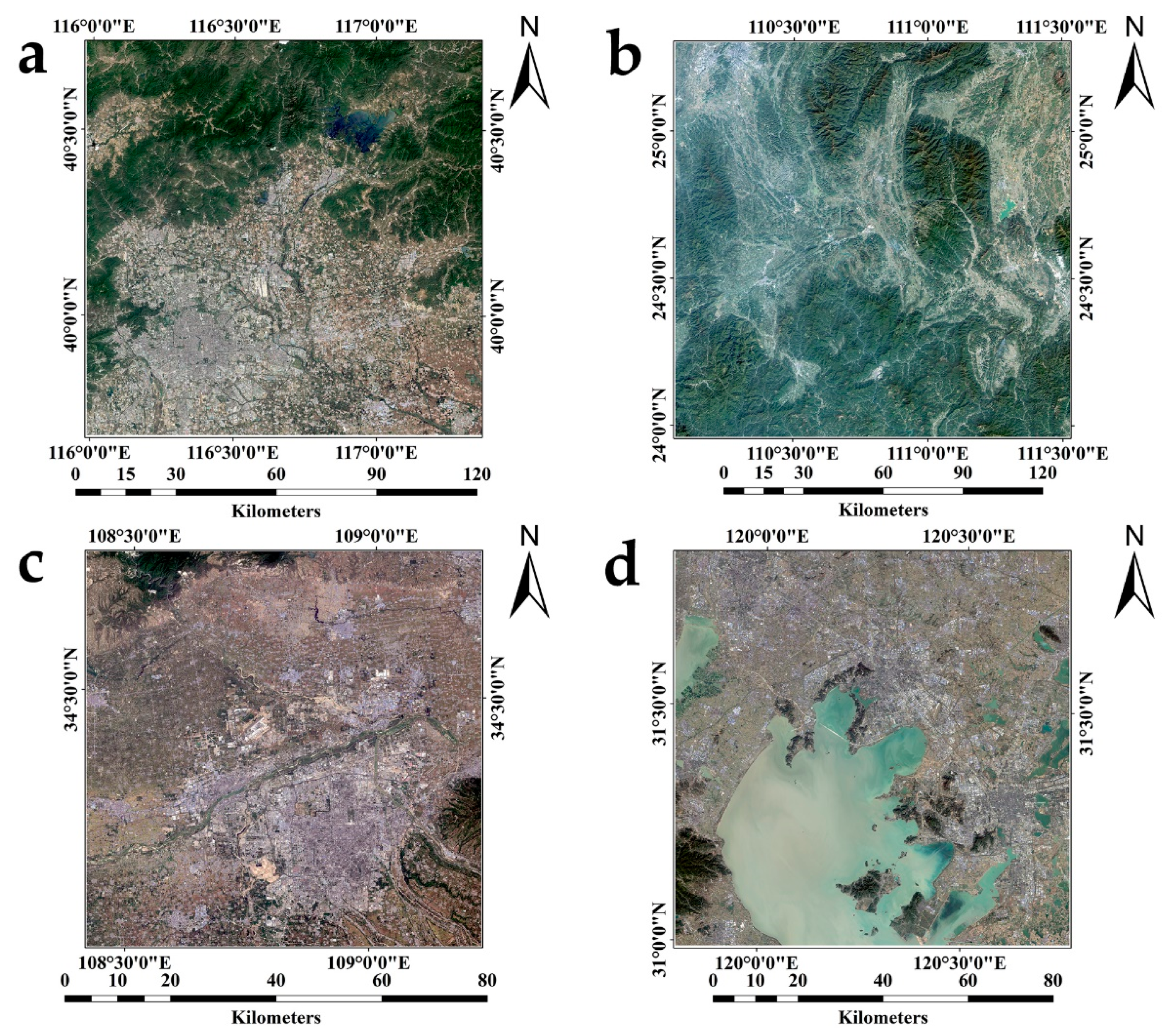
2.1. Study Sites

In order to compare and analyze the effects of the D-DisTrad, DisTrad, and TsHARP models under different scenarios, this paper mainly considers the effects of the geographical location, climate, economic conditions, topography, and land cover, and selects four representative sites within China. Firstly, these sites are separately located in northern, southern, western, and eastern China, and are also representative of the different climate types in China. Secondly, these sites have different levels of economic development and represent the most developed, average developed, emerging developed, and traditionally developed regions in China, respectively. Additionally, influenced by the geographical location, type of climate, and economic level, these sites have different topographic conditions and form different types of land cover. Among them, the topography of site 1 is predominantly hilly, site 2 is mountainous, site 3 is dominated by plains, and the topography of site 4 also contains plains. The land cover types of the four sites also have different characteristics. Site 1 is dominated by artificial surfaces; site 2 is mainly forests; site 3 is a mixture of artificial surfaces, bare land, and arable land; and site 4 is predominantly water bodies. The four sites are specifically described below (

Table 1. List of study sites and Landsat 8 and Sentinel-3 images used in this study.

Site	Imagining Date	Location	Landsat 8		Sentinel-3 OLCI	Sentinel3 SLSTR
			Path/Row	Overpass Time (UTC/GMT+08:00)
1	19 June 2021	Beijing	123/32	10:53:22	10:17:30
2	3 December 2021	Guilin	124/43	11:04:26	10:52:07
3	30 May 2021	Xi’an–Xian Yang	127/36	11:19:33	10:36:10
4	20 November 2021	Taihu River Basin	119/38	10:31:19	10:07:49

and Figure 1).

Simultaneously, in order to compare and analyze the effects of the above three models in different seasons, four seasons for site 2 and site 3 were selected for study in this paper (

Table 2. List of Sentinel-3 images used in site 2 and site 3.

Site	Location	Acquisition Date	Sentinel-3 OLCI	Sentinel3SLSTR
			Overpass Time (UTC/GMT+08:00)
2	Guilin	3 December 2021 (winter)	10:52:07
		8 March 2022 (spring)	10:27:56
		6 June 2021 (summer)	10:57:53
		22 October 2020 (fall)	10:42:49
3	Xi’an–Xian Yang	19 February 2021 (winter)	10:28:37
		8 May 2021 (spring)	11:07:44
		1 August 2021 (summer)	11:04:09
		10 November 2021 (fall)	10:45:23

). Site 3 was chosen for the reason that site 3 has four distinct seasons and was well placed to analyze the effects of the model on different seasonal characteristics. However, considering the diverse impacts of seasonality in urban and rural areas, site 3 was chosen to take into account the seasonal characteristics of urban areas only, so site 2 was chosen to compensate for site 3.

• Site 1—Beijing

Beijing, the capital of the People’s Republic of China, is one of China’s most populous and urbanized districts. It is also a first-tier metropolis globally [38]. Beijing is situated in northern China, with a high topography in the northwest and a low terrain in the southeast, consisting mainly of plains and mountains, with an average altitude of 43.5 m. The climate type is a warm, temperate, semi-humid, semi-arid monsoon climate, with an average annual temperature of 13.8 °C and average precipitation of 527.1 mm. There are also water bodies, arable land, grassland, and shrubland.

• Site 2—Guilin

Guilin is an important tourist city in China and also a famous international tourist city. It is located in the southwestern part of the South China Ridge Mountain System and in the middle of the northern part of the Guilin–Yangshuo Karst Basin, with a predominantly mesic or low mesic topography and large undulations. Guilin is also a typical karst landscape region in China [39]. Guilin has a subtropical monsoon climate, with an average annual temperature of 19.1 °C and average annual precipitation of 1887.6 mm, with a mild climate, abundant rainfall, four distinct seasons, basically the same seasons of rain and heat, and very favorable climatic conditions. The types of land cover are mainly artificial surfaces, forests, arable land, and water bodies.

• Site 3—Xi’an–Xian Yang

Site 3 is a representative emerging development area in China. The area is located in the interior of northwest China, on the secondary terraces of the Weihe Plain, with a flat topography and an average elevation of 400 m. It has a warm, temperate, semi-humid continental monsoon climate, with four distinct seasons, cold, warm, dry, and wet, with an average annual temperature of 15.2 °C and average precipitation of 648.2 mm. The types of land cover in the region are simple, mainly artificial surfaces, water bodies, and arable land.

• Site 4—Taihu River Basin

Taihu Lake is the third largest freshwater lake in China, with an area of 2427.8 square kilometers and a surface elevation of 3.33 m. Its western and southwestern sides are hilly and mountainous, while its eastern side is dominated by plains and water networks. Located at the southern edge of the Yangtze River Delta in eastern China, the basin contains several of the economically powerful cities in China. The Taihu Lake basin is located in the subtropical zone, with a mild and humid climate and a subtropical monsoon climate, with an average annual temperature of 16.0–18.0 °C and annual precipitation of 1100–1150 mm. The regional land cover is dominated by water bodies, with the presence of artificial surfaces, arable land, wetlands, and shrublands.

2.2. Data and Data Processing

The Sentinel-3 OLCI is a push-scan spectral imager with 21 bands and a spatial resolution of 300 m. The Sentinel-3 SLSTR is a dual-view scanning temperature radiometer capable of providing LST products with a spatial resolution of 1000 m. Both the OLCI image and the SLSTR image are from the Copernicus Open Access Hub (https://scihub.copernicus.eu/) (accessed on 2 June 2022). ASTER GDEM v3 image provides DEM data at a spatial resolution of 30 m from the Chinese Academy of Sciences Geospatial Data Cloud Platform (http://www.gscloud.cn/) (accessed on 2 June 2022). Landsat 8 images are available at a spatial resolution of 30 m in the multispectral band and 100 m in the thermal infrared band from the United States Geological Survey (https://earthexplorer.usgs.gov/) (accessed on 2 June 2022). In addition, MOD05_L2 products were obtained from the Level-1 and Atmosphere Archive and Distribution System Distributed Active Archive Center (LAADS DAAC) (https://ladsweb.modaps.eosdis.nasa.gov/) (accessed on 2 June 2022).

The pre-processing of ASTER GDEM images and Landsat-8 images was accomplished using Envi5.3 software and Complete MOD05_L2 water vapor products with the Modis Conversion Toolkit software. The pre-processing for Sentinel-3 OLCI and SLSTR images was done using the Sentinel applications platform (Snap) software. Among these data, the ASTER GDEM images were aggregated to resolutions of 300 and 900 m, and NDVI, NDWI, and BI2 images were calculated using OLCI images aggregated to a resolution of 900 m, which were used to construct high- and low-resolution influence factors. The SLSTR images were resampled to a resolution of 900 m, as 900 m is an integer multiple of 30 m for Landsat 8 and 300 m for OLCI images, making them easy to compare and analyze. The LST data retrieved from Landsat 8 were aggregated to a 300 m resolution to validate the 300 m downscaling results. The LST data generated from three downscaling models were aggregated to the 900 m resolution and evaluated in comparison with the resampled SLSTR LST products. Furthermore, the geometric correction of Sentinel-3 images was carried out using Landsat 8 images as the reference [40].

3. Methods

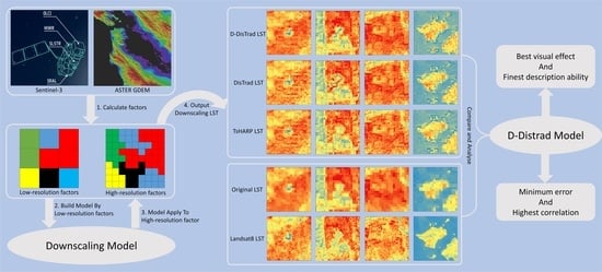
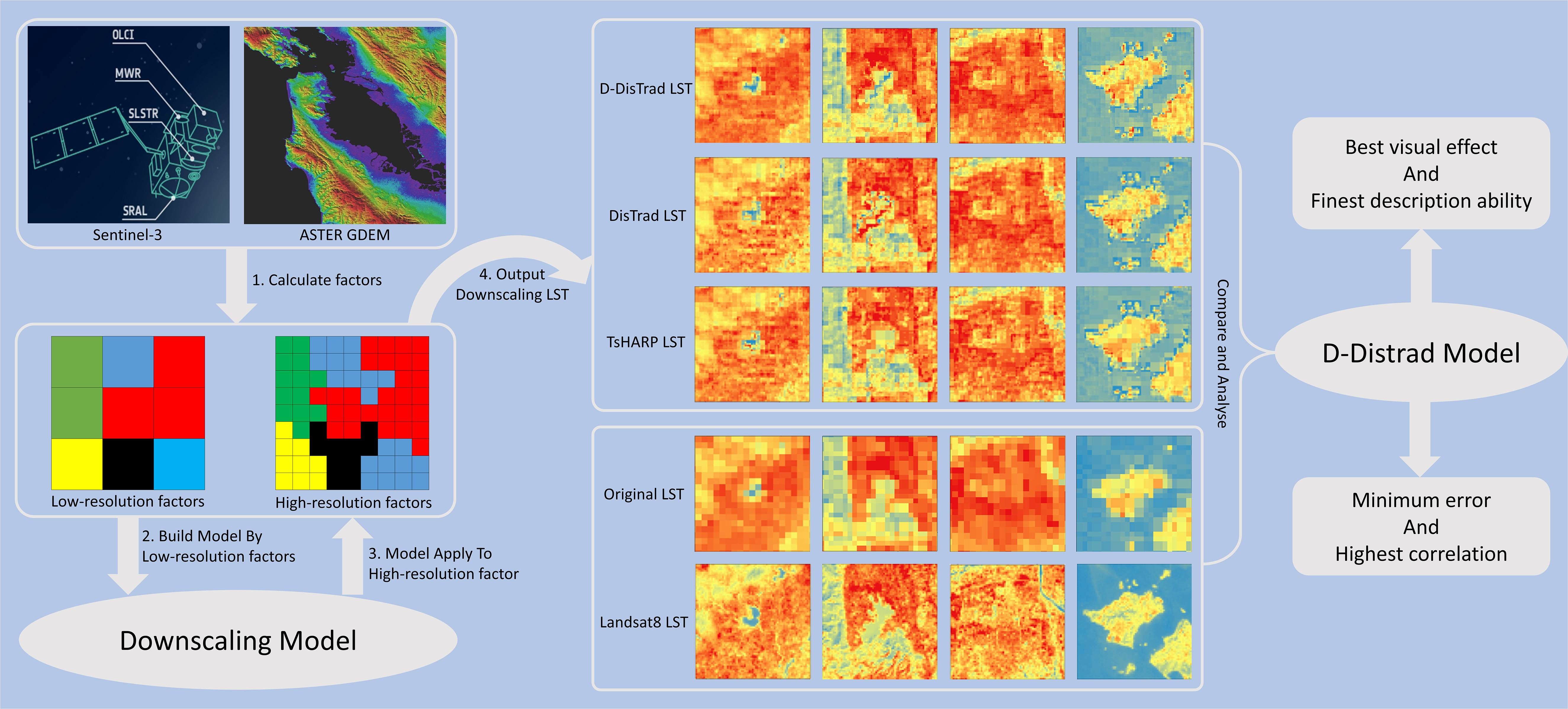
3.1. Downscaling Model

The basic principle of the LST downscaling of statistics-based methods is scale invariance; that is, there is a certain quantitative relationship between LST data and influence factors at different spatial resolutions [22]. Specifically, a quantitative model of LST and influence factors is developed at the low spatial resolution, and this model is then applied to the high-resolution influence factors to produce high spatial resolution LST data. Since the selected influence factors may not necessarily fully satisfy the downscaling requirements under various conditions, and as there is also a large amount of heterogeneity in the land cover, there are inevitable residuals between the actual and predicted results generated based on the model [41]. Thus, finally, the residuals have to be spatially redistributed and appended to the prediction results to produce high spatial resolution LST downscaling data with higher accuracy. The mathematical model of the LST downscaling can be described as follows (Equations (1)–(3)):

$${\mathrm{LST}}_{\mathrm{coarse}}{=\mathrm{f}(\mathrm{IF}}_{\mathrm{coarse}})$$

(1)

$${\mathrm{LST}}_{\mathrm{residuals}}{=\mathrm{LST}}_{\mathrm{origin} }{– \mathrm{LST}}_{\mathrm{coarse}}$$

(2)

$${\mathrm{LST}}_{\mathrm{fine}}=\mathrm{f}\left({\mathrm{IF}}_{\mathrm{fine}}\right){+\mathrm{LST}}_{\mathrm{fine}\_\mathrm{residuals}}$$

(3)

where ${\mathrm{LST}}_{\mathrm{coarse}}$ is the predicted low-resolution LST data using the downscaling model, f is a function of the downscaling model, ${\mathrm{IF}}_{\mathrm{coarse}}$ is the low-resolution influence factor, ${\mathrm{LST}}_{\mathrm{origin}}$ represents the actual LST images, ${\mathrm{LST}}_{\mathrm{residuals}}$ represents the residual between the predicted low-resolution LST data and the actual LST images, ${\mathrm{IF}}_{\mathrm{fine}}$ represents the high-resolution influence factor, ${\mathrm{LST}}_{\mathrm{fine}\_\mathrm{residuals}}$ represents the residual of the resampling to high resolution, and ${\mathrm{LST}}_{\mathrm{fine}}$ represents the downscaled (high-resolution) LST data.

Nowadays, the DisTrad model and TsHARP model are commonly used and are effective downscaling models for LST data. The DisTrad model is based on the linear relationship between the LST and NDVI, and its downscaling model relationship ${\mathrm{f}}_{\mathrm{DisTrad}}$ is expressed as Equations (4) and (5):

$${\mathrm{f}}_{\mathrm{DisTrad}} : \mathrm{LST}=\mathrm{a} \times \mathrm{NDVI}+\mathrm{b}$$

(4)

$$\mathrm{NDVI}=\frac{\mathrm{Oa}17 - \mathrm{Oa}08}{\mathrm{Oa}17+\mathrm{Oa}08}$$

(5)

where a and b are the constant coefficients obtained by fitting a linear regression to NDVI and LST data, and $\mathrm{Oa}17$ and $\mathrm{Oa}08$ represent band 17 and band 8 of the Sentinel-3 OLCI sensor.

The TsHARP model is based on the DisTrad model, which uses the FVC instead of the NDVI and LST to establish a downscaling model relationship ${\mathrm{f}}_{\mathrm{TsHARP}}$, as follows (Equations (6) and (7)):

$${\mathrm{f}}_{\mathrm{TsHARP}} : \mathrm{LST}=\mathrm{a} \times \mathrm{FVC}+\mathrm{b}$$

(6)

$$\mathrm{FVC}=1 – ( \frac{{\mathrm{NDVI}}_{\max } {– \mathrm{NDVI}}_{\mathrm{i}}}{{\mathrm{NDVI}}_{\max }{– \mathrm{NDVI}}_{\min }}{ )}^{0.625}$$

(7)

where a and b are the constant coefficients obtained by fitting a linear regression to FVC and LST, ${\mathrm{NDVI}}_{\copyright }$ represents the NDVI value for a given pixel, and ${\mathrm{NDVI}}_{\min }$ and ${\mathrm{NDVI}}_{\max }$ represent the minimum and maximum NDVI values corresponding to a confidence interval range of 5% to 95%, respectively.

The above two linear models are more suitable for a single vegetation cover area, whereas in reality land covers also include artificial surfaces, water bodies, and bare soil. One must also take into account the relationship between the radiant energy received by the ground and the elevation. Therefore, the D-DisTrad model proposed in this paper takes the NDVI, NDWI, BI2, and DEM as independent variable influence factors, and establishes the multivariate linear regression relationship model ${\mathrm{f}}_{\mathrm{D-DisTrad}}$ with the LST (Equations (8)–(10)).

$${\mathrm{f}}_{\mathrm{D-DisTrad} }: \mathrm{LST}=\mathrm{a} \times \mathrm{NDVI}+\mathrm{b} \times \mathrm{NDWI}+\mathrm{c} \times \mathrm{BI}2+\mathrm{d} \times \mathrm{DEM}+\mathrm{e}$$

(8)

$$\mathrm{NDWI}=\frac{\mathrm{Oa}06 - \mathrm{Oa}17}{\mathrm{Oa}06+\mathrm{Oa}17}$$

(9)

$$\mathrm{BI}2=\sqrt{\frac{{\left(\mathrm{Oa}08\right)}^2{+\left(\mathrm{Oa}06\right)}^2{+\left(\mathrm{Oa}17\right)}^2}{3}}$$

(10)

where a, b, c, d, and e are the constant coefficients obtained by fitting a linear regression to the NDVI, NDWI, BI2, DEM, and LST, and $\mathrm{Oa}06$ represents band 6 of the Sentinel-3 OLCI sensor.

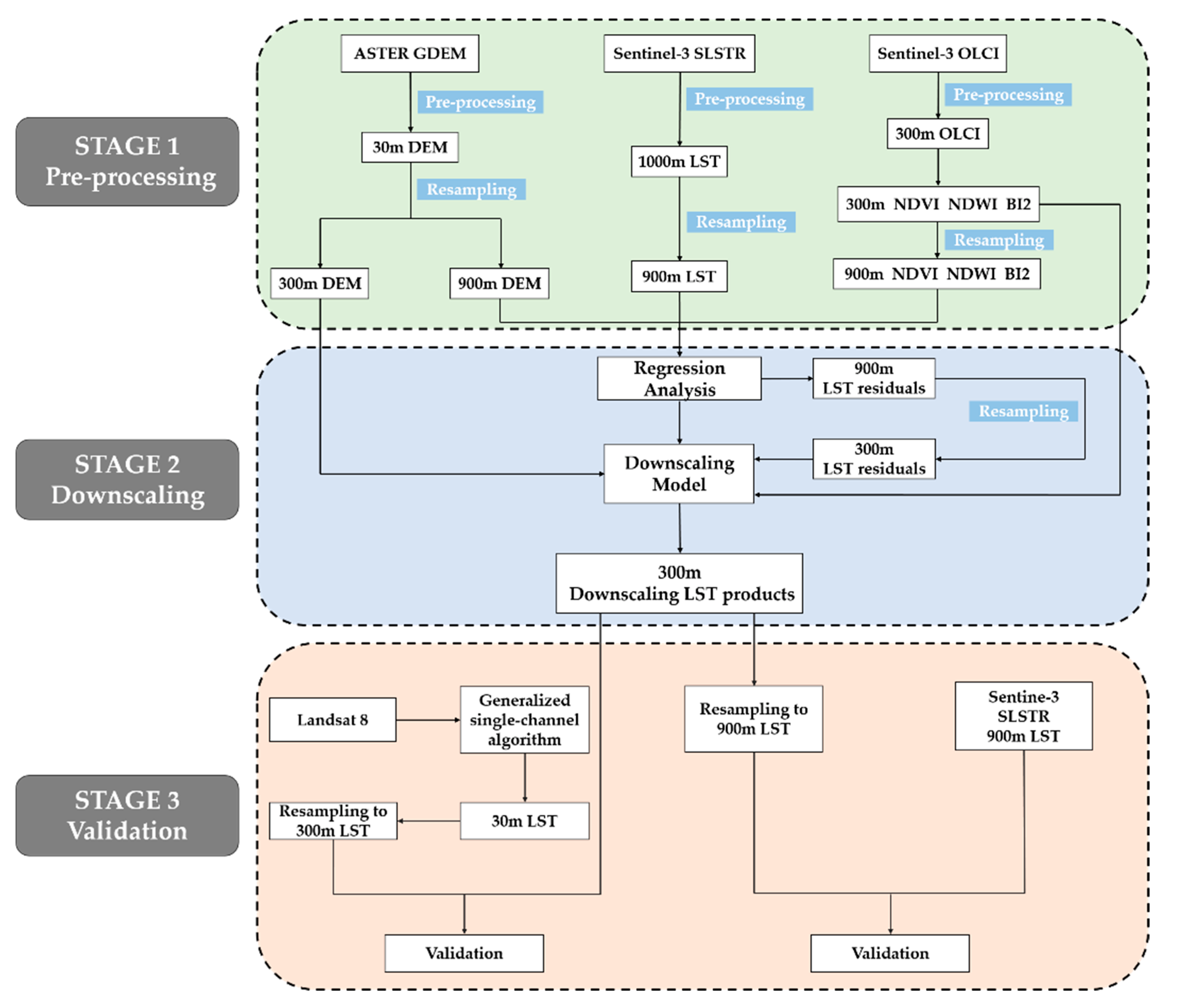
3.2. Methodological Workflow

Sentinel-3 OLCI, SLSTR, and ASTER GDEM data were pre-processed to construct the DisTrad, TsHARP, and D-DisTrad models to produce downscaled LST data. The LST data after downscaling were compared with Sentinel-3 SLSTR LST images and the LST data retrieved from Landsat 8 images, then the accuracy of the three models was evaluated. This process was divided into three stages (Figure 2).

Sentinel-3 OLCI, SLSTR, and ASTER GDEM data were preprocessed in stage 1 to produce influence factors with the high and low spatial resolutions needed for downscaling. Stage 2 involved the creation of DisTrad, TsHARP, and D-DisTrad downscaling models using the stage 1 influence factors, generating downscaled LST data using the three models. In stage 3 we evaluated the downscaled LST data using the LST data generated from Landsat 8 inversion and Sentinel 3 SLSTR LST images, and compared and evaluated the actual effects and accuracy of the three models.

3.3. Generalized Single-Channel Algorithm

In this paper, LST data retrieved from Landsat 8 were utilized for the evaluation of the results. The inversion methods used for LST data from Landsat 8 images mainly include single-channel and split-window algorithms. In the author’s previous work experience, the generalized single-channel algorithm had better inversion accuracy, and many studies have shown that it can achieve good results [42,43,44], so this algorithm was used in this research (Equations (11) and (12)) [45]:

$$\left\{\begin{array}{c}{\mathrm{T}}_{\mathrm{s}}=\gamma \left(\frac{{\psi }_1{\mathrm{L}}_{\mathrm{sen}}{+\psi }_2}{\epsilon }{+\psi }_3\right)+\delta \\ \gamma =\frac{{\mathrm{T}}_{\mathrm{sen}}^2}{{(\mathrm{b}}_{\gamma }{\mathrm{L}}_{\mathrm{sen}})} {, \delta =\mathrm{T}}_{\mathrm{sen}} – \frac{{\mathrm{T}}_{\mathrm{sen}}^2}{{\mathrm{b}}_{\gamma }}\end{array}\right.$$

(11)

$$\left\{\begin{array}{c}{\psi }_1{=\mathrm{c}}_{11}{\mathrm{w}}^2{+\mathrm{c}}_{12}{\mathrm{w}+\mathrm{c}}_{13}\\ {\psi }_2{=\mathrm{c}}_{21}{\mathrm{w}}^2{+\mathrm{c}}_{22}{\mathrm{w}+\mathrm{c}}_{23}\\ {\psi }_3{=\mathrm{c}}_{31}{\mathrm{w}}^2{+\mathrm{c}}_{32}{\mathrm{w}+\mathrm{c}}_{33}\end{array}\right.$$

(12)

where ${\mathrm{T}}_{\mathrm{s}}$ is the surface temperature (K); $\gamma$ and $\delta$ are the correlation coefficients of the Planck equation ${\psi }_1$,${\psi }_2$, and ${\psi }_3$ are functions of atmospheric water vapor $\mathrm{w}$; ${\mathrm{b}}_{\gamma }$ is a fixed value equal to 1324 K; ${\mathrm{L}}_{\mathrm{sen}}$ is the on-star radiance; $\epsilon$ is the land surface emissivity; ${\mathrm{T}}_{\mathrm{sen}}$ is the bright temperature on the star; and ${\mathrm{c}}_{\mathrm{ij}}$ is a series of fixed values (

Table 3. The values of parameter ${\mathrm{c}}_{\mathrm{ij}}$ in the generalized single-window algorithm.

Sensor	${\mathbf{c}}_{\mathbf{ij}}$	j = 1	j = 2	j = 3
Landsat 8 TIRS	i = 1	0.04019	0.02916	1.01523
	i = 2	−0.38333	−1.50294	0.20324
	i = 3	0.00918	1.36072	−0.27514

) [46].

The atmospheric water vapor $\mathrm{w}$ is acquired from the MOD05_ L2 product.

Due to the necessity of using Landsat-8 data for the accuracy evaluation of Sentinel-3 data and different LST products using different empirical methods to describe the emissivity [47], it would be good to control for these factors in the validation. Through the ESA presentation of the Sentinel-3 SLSTR, it is only possible to know that the algorithm of the Sentinel-3 LST data implicitly takes into account the effect of the surface emissivity via the biome and fractional vegetation and calculates the types of surface backgrounds. Hence, to keep the surface emissivity as consistent as possible, the surface emissivity $\epsilon$ calculation method proposed by Qin et al., which takes into account the mixed image elements and the type of surface cover, is used as follows (Equations (13)–(16)) [48]:

$${\mathrm{P}}_{\mathrm{v}}=(\frac{{\mathrm{NDVI} - \mathrm{NDVI}}_{\min }}{{\mathrm{NDVI}}_{\max }{ - \mathrm{NDVI}}_{\min }}{)}^2$$

(13)

$${\epsilon =\mathrm{P}}_{\mathrm{v}}{\mathrm{R}}_{\mathrm{v}}{\epsilon }_{\mathrm{v} }{+(1 - \mathrm{P}}_{\mathrm{v}}{)\mathrm{R}}_{\mathrm{s}}{\epsilon }_{\mathrm{s}}+\mathrm{d}\epsilon (\mathrm{natural} \mathrm{surface})$$

(14)

$${\epsilon =\mathrm{P}}_{\mathrm{v}}{\mathrm{R}}_{\mathrm{v}}{\epsilon }_{\mathrm{v}}{+(1 - \mathrm{P}}_{\mathrm{v}}{)\mathrm{R}}_{\mathrm{m}}{\epsilon }_{\mathrm{m}}+\mathrm{d}\epsilon (\mathrm{man-made} \mathrm{surface})$$

(15)

$$\left\{\begin{array}{c}{\mathrm{R}}_{\mathrm{v}}=0.9332+0{.0585\mathrm{P}}_{\mathrm{v}}\\ {\mathrm{R}}_{\mathrm{s}}=0.9902+0{.1068\mathrm{P}}_{\mathrm{v}}\\ {\mathrm{R}}_{\mathrm{m}}=0.9886+0{.1287\mathrm{P}}_{\mathrm{v}}\end{array}\right.$$

(16)

where ${\mathrm{P}}_{\mathrm{v}}$ is vegetation fraction of the surface, with $0 \le { \mathrm{P}}_{\mathrm{v}} \le 1$, NDVI represents the NDVI value for a given pixel, and ${\mathrm{NDVI}}_{\min }$ and ${\mathrm{NDVI}}_{\max }$ represent the minimum and maximum NDVI values corresponding to a confidence interval of 5% to 95%.${ \mathrm{R}}_{\mathrm{v}}$, ${\mathrm{R}}_{\mathrm{s}}$, and ${\mathrm{R}}_{\mathrm{m}}$ are radiance ratios of the vegetation, bare soil, and buildings, respectively; the values of ${\epsilon }_{\mathrm{v}}$, ${\epsilon }_{\mathrm{s}}$, and ${\epsilon }_{\mathrm{m}}$ are 0.986, 0.97215, and 0.970, respectively; dε = 0 when the surface is flat, and when the surface is highly undulating, a simple estimate can be made based on the value of ${\mathrm{P}}_{\mathrm{v}}$ [48].

3.4. Downscaling Model Performance Evaluation

Two types of analyses are performed to evaluate the effects of the downscaling model. The first type of analysis is qualitative. By directly comparing the spatial differences between the downscaling results and the actual results, this method cannot get the numerical differences between the two data types. The quantitative analysis is the second type. The quantitative analysis is divided into two steps. The first step is to aggregate Landsat 8 LST to the 300 m spatial resolution and compare the quantitative relationship between it and the three 300 m downscaled LST data types. However, since the overpass times of Landsat 8 deviates somewhat from Sentinel-3 (Table 1) and solar radiation may change within a short time, causing changes in surface temperature, the two do not necessarily match exactly. This kind of method is more a matter of assessing the trends between two data points. In contrast, another kind of method aggregates 300 m downscaling LST to 900 m for the quantitative analysis with Sentinel-3 SLSTR LST images [28].

The quantitative analysis is accomplished through five indicators: the mean bias ($\mathrm{MB}$), mean absolute error (MAE), root mean square error (RMSE), Pearson correlation coefficient (PCC), and coefficient of determination (${\mathrm{R}}^2$) (Equations (17)–(21)):

$$\mathrm{MB}=\frac{{{\displaystyle \sum }}_{\mathrm{i}=1}^{\mathrm{n}}{(\mathrm{LST}}_{\mathrm{pre}}{ – \mathrm{LST}}_{\mathrm{actual}})}{\mathrm{n}}$$

(17)

$$\mathrm{MAE}=\frac{{{\displaystyle \sum }}_{\mathrm{i}=1}^{\mathrm{n}}\left|{(\mathrm{LST}}_{\mathrm{pre}}{ – \mathrm{LST}}_{\mathrm{actual}})\right|}{\mathrm{n}}$$

(18)

$$\mathrm{RMSE}=\sqrt{\frac{{{\displaystyle \sum }}_{\mathrm{i}=1}^{\mathrm{n}}{{(\mathrm{LST}}_{\mathrm{pre}}{ – \mathrm{LST}}_{\mathrm{actual}})}^2}{\mathrm{n}}}$$

(19)

$$\mathrm{PCC}=\frac{{{\displaystyle \sum }}_{\mathrm{i}=1}^{\mathrm{n}}{(\mathrm{LST}}_{\mathrm{pre}} – \overline{{\mathrm{LST}}_{\mathrm{pre}}}{\left)\right(\mathrm{LST}}_{\mathrm{actual}} – \overline{{\mathrm{LST}}_{\mathrm{actual}}})}{\sqrt{{{\displaystyle \sum }}_{\mathrm{i}=1}^{\mathrm{n}}{{(\mathrm{LST}}_{\mathrm{pre}} – \overline{{\mathrm{LST}}_{\mathrm{pre}}})}^2}\sqrt{{{\displaystyle \sum }}_{\mathrm{i}=1}^{\mathrm{n}}{{(\mathrm{LST}}_{\mathrm{actual}} – \overline{{\mathrm{LST}}_{\mathrm{actual}}})}^2}}$$

(20)

$${\mathrm{R}}^2=\frac{{{\displaystyle \sum }}_{\mathrm{i}=1}^{\mathrm{n}}{{(\mathrm{LST}}_{\mathrm{pre}} – \overline{{\mathrm{LST}}_{\mathrm{actual}}})}^2}{{{\displaystyle \sum }}_{\mathrm{i}=1}^{\mathrm{n}}{{(\mathrm{LST}}_{\mathrm{actual}} – \overline{{ \mathrm{LST}}_{\mathrm{actual}}})}^2}$$

(21)

where ${\mathrm{LST}}_{\mathrm{pre}}$ is the downscaling LST value of a pixel, $\overline{{\mathrm{LST}}_{\mathrm{pre}}}$ is the average of the downscaling LST values of all pixels, ${\mathrm{LST}}_{\mathrm{actual}}$ is the actual LST value of a pixel, and $\overline{{\mathrm{LST}}_{\mathrm{actual}}}$ is the average of the actual LST values of all pixels.

4. Results

4.1. Qualitative Evaluation

The qualitative evaluation is used to visually analyze whether the results after downscaling can retain the spatial distribution of the LST more accurately and finely with improved spatial resolution. The performance of the downscaling model is evaluated by comparing the differences in spatial distribution between the downscaling LST and Sentinel-3 SLSTR LST and Landsat 8 LST data. The qualitative evaluation of the different sites was carried out by aggregating Landsat 8 LST data to a spatial resolution of 300 m and then comparing them with the 300 m LST generated from three downscaling models, as well as the Sentinel-3 SLSTR LST data at 900 m to analyze the spatial distribution. The evaluation of different seasons is mainly performed to compare SLSTR LST data with three downscaling images.

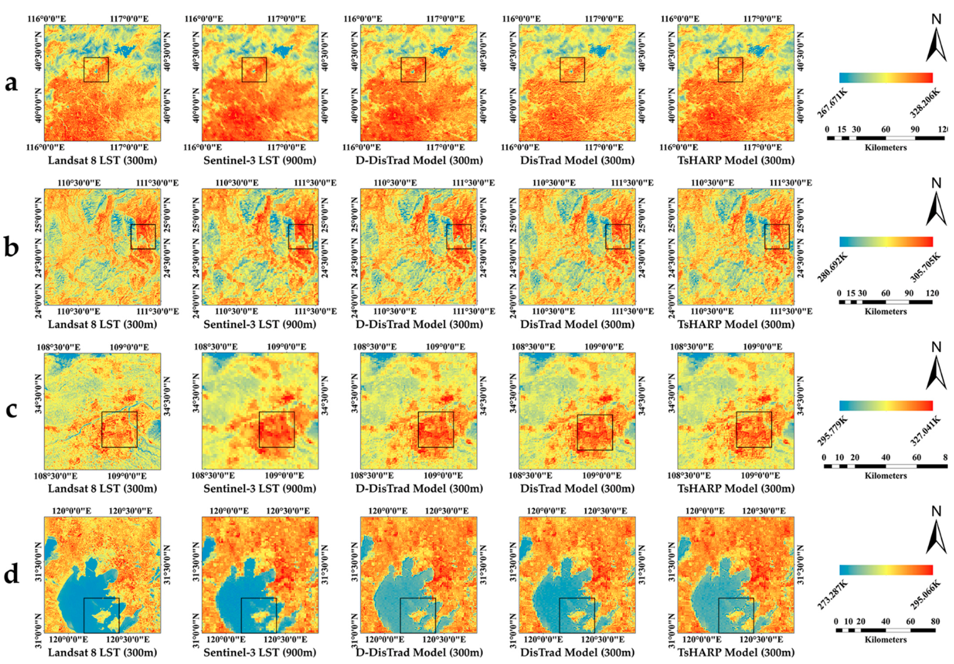
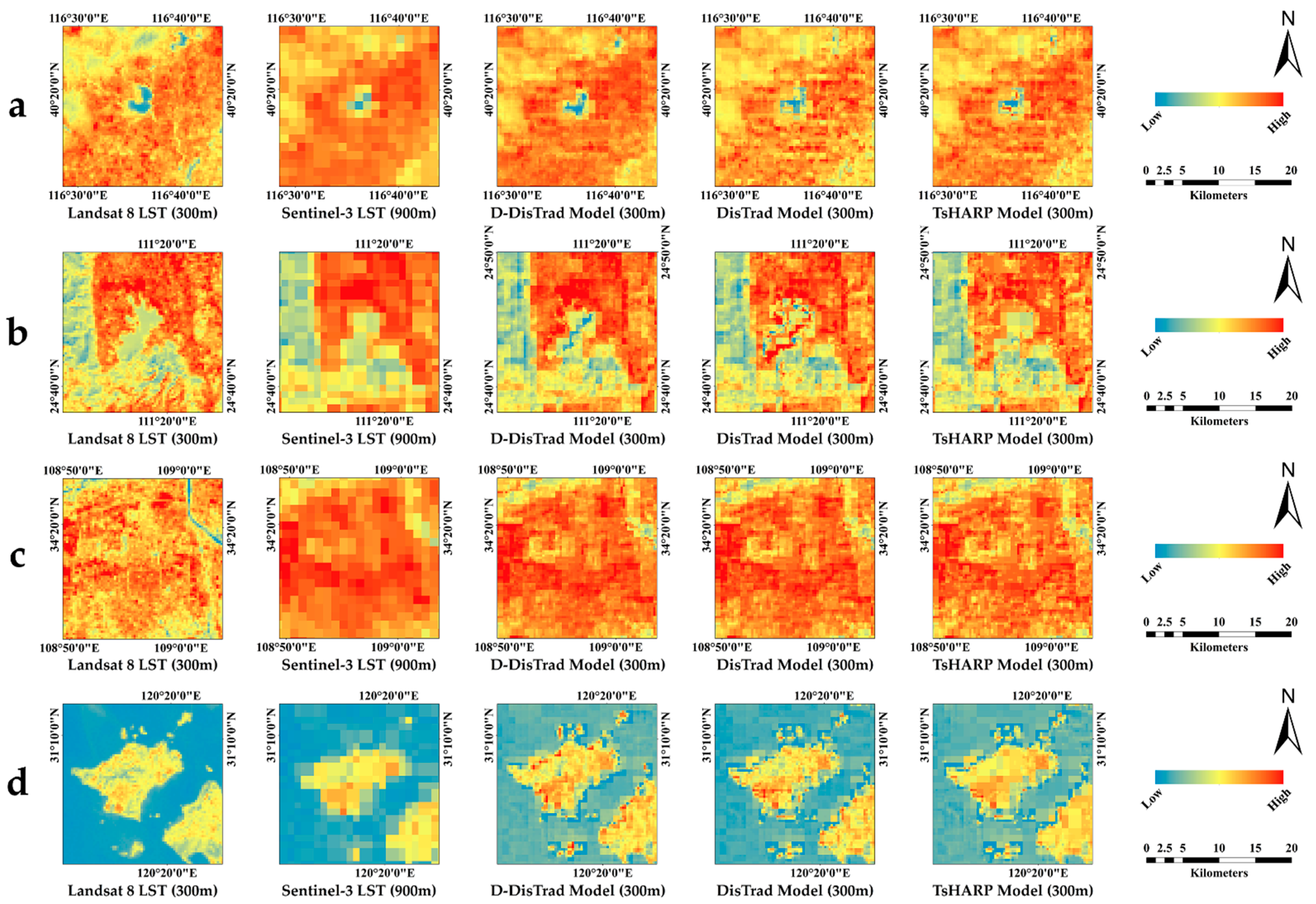
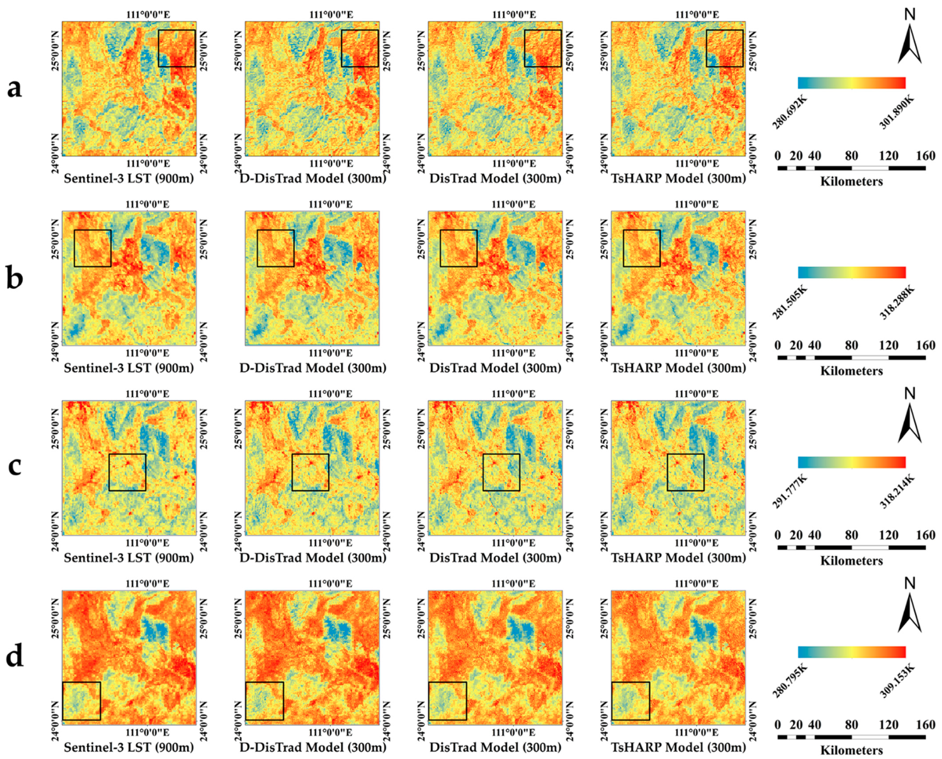
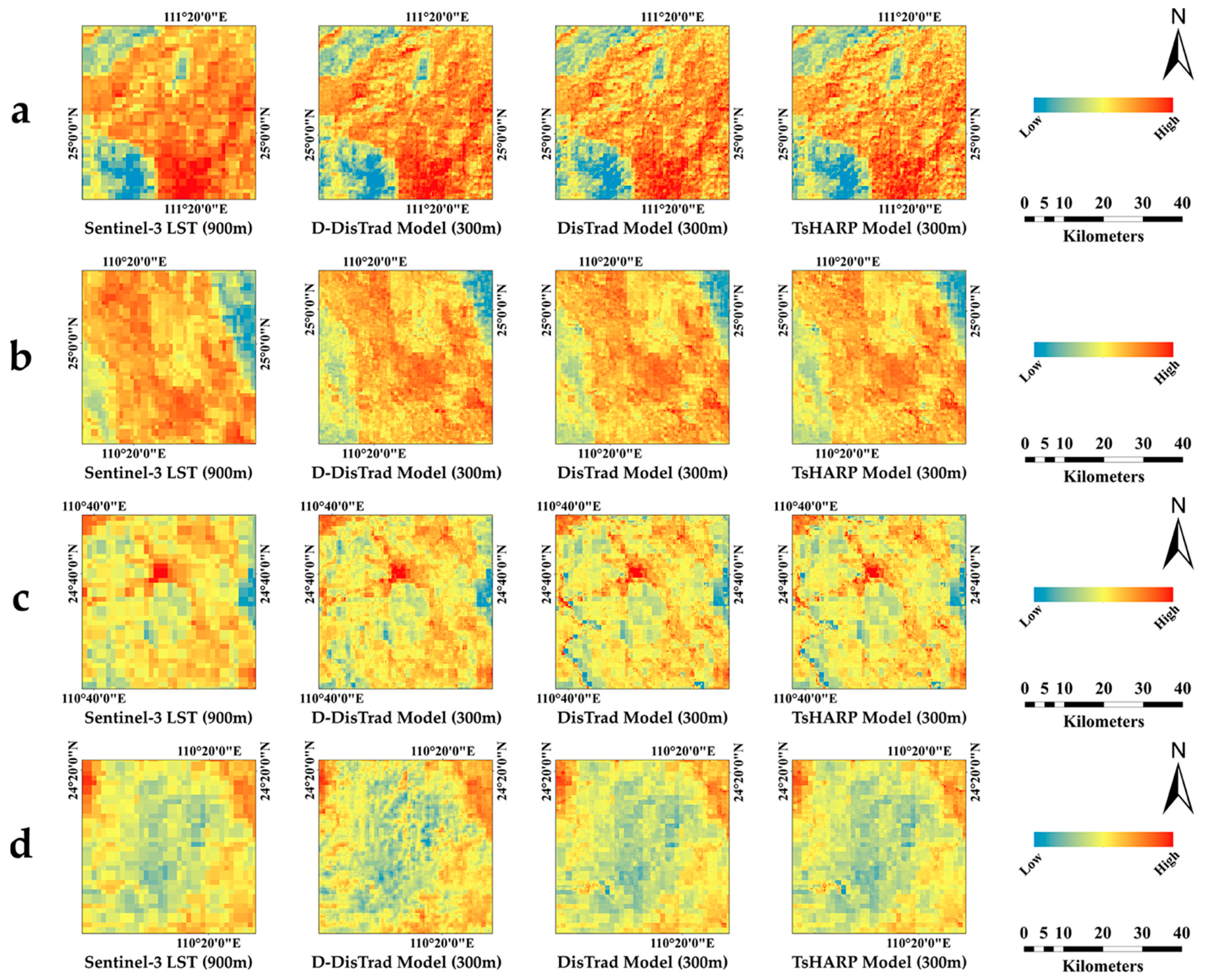
4.1.1. Qualitative Evaluation of Different Sites

In order to better present the results of the qualitative evaluation, each site is graded and colored separately. It is necessary to note that although the color bars of the different sites are the same color, the range of values represented by each color bar is different. The same color at different sites does not represent the same value, and the colors cannot be compared directly between sites. This avoids the possibility that images with a small temperature range may only show a single color when all images use the same color range. Figure 3 shows the Landsat LST, SLSTR LST, and three downscaling results at different sites.

To better demonstrate and compare the visual results before and after downscaling, an area with noticeable changes was selected from each study site, as shown in Figure 4.

For the four selected study sites, all three downscaling methods achieved the downscaling task for the Sentinel-3 SLSTR LST images, which obviously improved the spatial texture details of the original LST images. These LST downscaling data showed similar results, which could better ensure the consistency of the LST data in terms of the spatial distribution before and after downscaling. Compared with the Landsat 8 LST data, the three downscaling data types remained fundamentally the same in their hue and distribution, but were slightly inferior to Landsat 8 LST data in the description of spatially detailed textures (mainly rivers). In comparison to the Sentinel-3 SLSTR LST data, the three downscaling data types describe the hue, spatial distribution, and spatial texture of LST data more finely and more accurately.

Specifically, the downscaling data generated by the D-DisTrad model is able to better describe the spatial texture information and highlight the differences in LST between different topographic and land cover features. This is mainly due to the introduction of multiple influence factors in the D-DisTrad model. In contrast, both the DisTrad and TsHARP models are essentially based on the NDVI, which can only reveal the general differences in vegetation cover and cannot better represent the spatial heterogeneity of LST data.

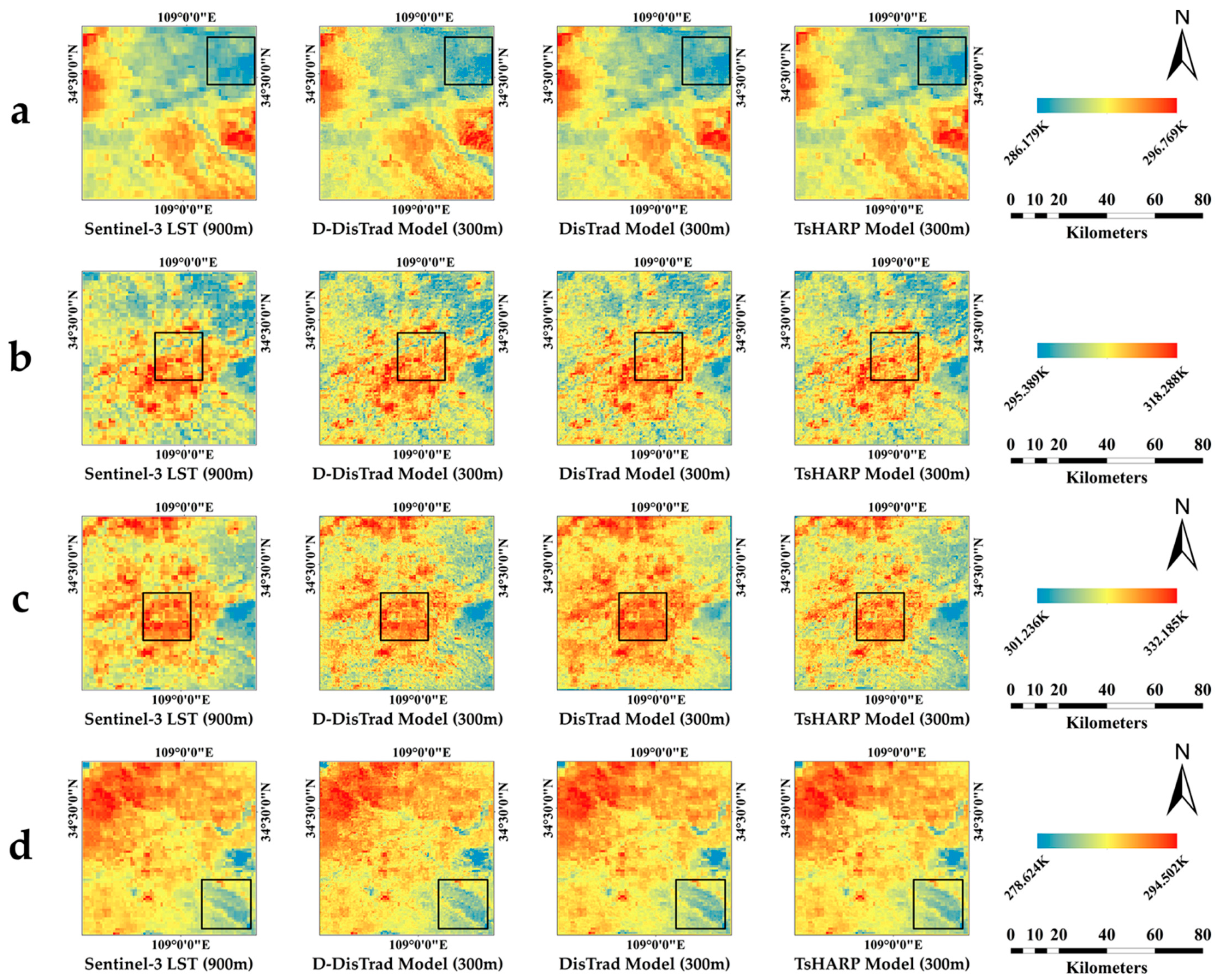
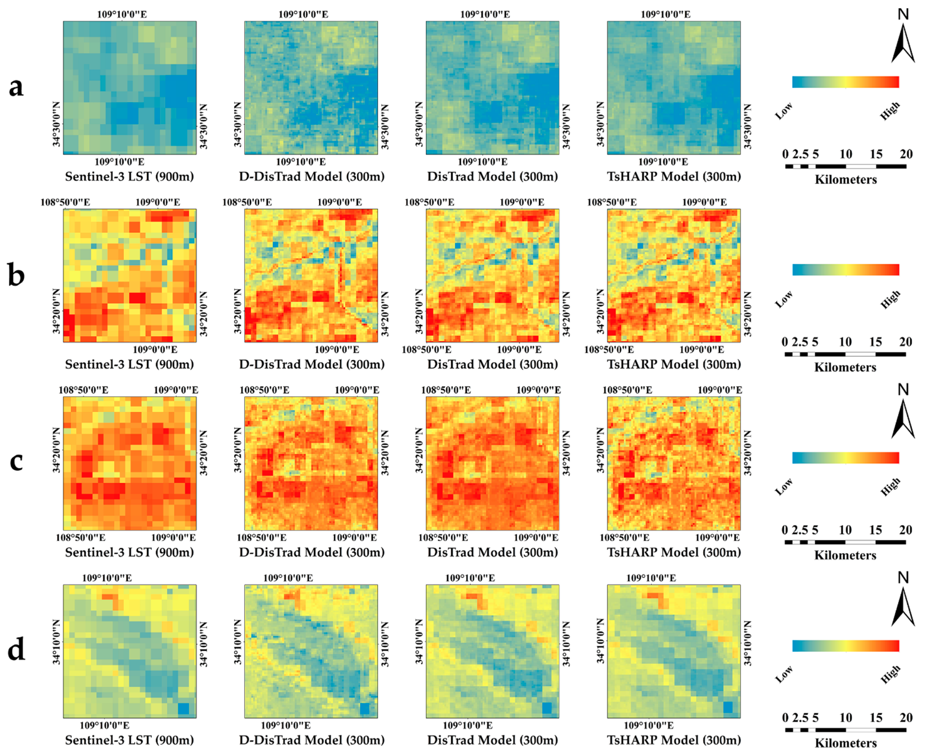
4.1.2. Qualitative Evaluation of Different Seasons

Figure 5 shows the LST images of site 3 in four different seasons, from which it can be seen that all three downscaling methods accomplish the task of downscaling in different seasons, improving the texture and detail of the original LST image and showing similar results, as well as maintaining the consistency of the spatial distribution of the LST image before and after downscaling. Specifically, the downscaled images generated by the D-DisTrad model also perform better, with a clearer depiction of texture and detail information (Figure 6 shows the areas selected with noticeable changes in four seasons), which is also due to the multiple factors introduced by the model. However, it is worth noting that the downscaling results for spring and summer are visually superior to those for autumn and winter. The spatial texture and detail of the downscaling results in spring and summer are clearer, and the differences in the spatial distribution of the LST are more pronounced. Although the images were also enhanced in the fall and winter seasons, the enhancement was not as effective as it was in the spring and summer seasons.

Figure 7 shows LST images of site 2 in four different seasons. Similar to site 3, all three downscaling models perform the task of downscaling across the different seasons for site 2, achieving both the preservation and enhancement of the image quality. Likewise, the downscaled images generated by the D-DisTrad model also show superior performance, with a clearer depiction of the texture and detail information (Figure 8 shows the areas selected with noticeable changes across the four seasons). Unlike site 3, however, the visual effects of site 2’s downscaled results are generally similar across the four seasons, and there is no one season where the visual effects of the images are significantly enhanced.

Overall, the results of the qualitative evaluation of the downscaling model in different seasons are generally similar to those of the qualitative evaluation of the different sites, but there may be some differences in the performance of the downscaling model in different seasons and different areas (urban or rural).

The qualitative evaluation reveals that the visual effect is enhanced by the downscaling of the LST from 1000 m to 300 m and the “mosaic” effect is eliminated effectively. For example, the Wei and Ba rivers in Figure 6b are clearly visible after downscaling; areas within the city with lower surface temperatures, such as the Daminggong National Park and the Han Chang’an City ruins in Figure 4c and Figure 6c, are also well distinguished. This additional information comes from the downscaling process, and the results are in better agreement with both the higher resolution images and the actual conditions.

Additionally, it is not a rigorous approach to determine the effect of the model using a visual qualitative evaluation alone, so a quantitative evaluation is required.

4.2. Quantitative Evaluation

Quantitative evaluation of downscaling results by calculating MB, MAE, RMSE, PCC and ${\mathrm{R}}^2$ between downscaling data and images (Landsat 8 LST or Sentinel-3 SLSTR LST).

4.2.1. Comparison with Landsat 8 LST Data

The Landsat 8 LST image at 300 m resolution was regressed against three downscaled LST images separately. Since the overpass times for Landsat 8 and Sentinel-3 are different, the analysis in this section mainly indirectly verifies the LST value quantitatively, so it mainly shows the results of the above five evaluation indicators (

Table 4. Statistics for the three downscaling results (300 m) in comparison with Landsat 8 LST data for 4 sites.

Indicator	Model	Site
		Beijing	Guilin	Xi’an–Xian Yang	Taihu Rive Basin
MB/K	D-DisTrad	1.728	−0.156	−0.795	0.510
	DisTrad	1.698	−0.143	−0.787	0.522
	TsHARP	1.626	−0.170	−0.576	0.501
MAE/K	D-DisTrad	2.189	1.067	1.633	0.898
	DisTrad	2.292	1.109	1.621	0.931
	TsHARP	2.356	1.100	1.520	0.913
RMSE/K	D-DisTrad	2.789	1.409	2.011	1.011
	DisTrad	2.955	1.461	1.997	1.151
	TsHARP	3.021	1.451	1.974	1.134
PCC	D-DisTrad	0.888	0.767	0.729	0.905
	DisTrad	0.858	0.750	0.731	0.878
	TsHARP	0.837	0.746	0.702	0.892
$R^2$	D-DisTrad	0.774	0.582	0.531	0.812
	DisTrad	0.723	0.551	0.534	0.774
	TsHARP	0.689	0.544	0.511	0.781

The bold font indicates the optimal value.

).

The results show that among the four study sites in this paper, firstly for the MB indicator, the DisTrad and D-DisTrad models exhibit relatively close results, and the TsHARP model shows the best results with the smallest average LST error reflected. For the other four indicators, except for site 3 in Xi’an–Xian Yang, the D-DisTrad model displays the lowest error, highest correlation, and best fit. In site 3, the TsHARP model has the lowest correlation and fit with the lowest error, while the DisTrad model has the best correlation and fit, and is close to the TsHARP model in the three error indicators. In general, the D-DisTrad model performed relatively well on all indicators but also had shortcomings, whereas the TsHARP and DisTrad models had their pros and cons. However, due to the imaging differences between the two platforms, assessing the most realistic and specific effects of the three models requires further validation in Section 4.2.2.

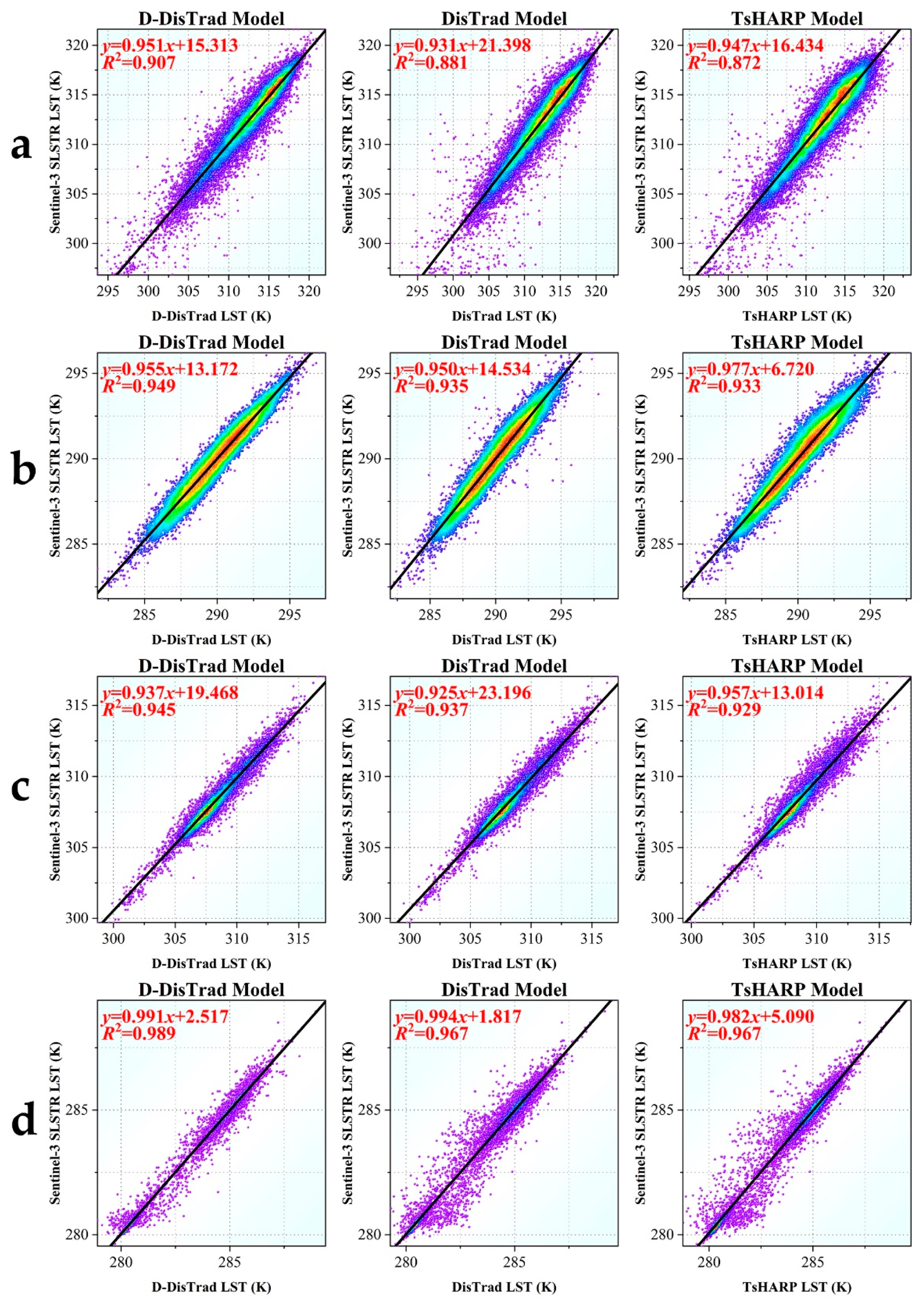
4.2.2. Comparison with Sentinel-3 SLSTR LST Data

To compare the downscaling effects at the different sites and in different seasons, the LST data generated by three downscaling models were aggregated to a resolution of 900 m and regressed with the Sentinel-3 SLSTR LST data at 900 m resolution, respectively. The five indicators mentioned above were calculated and are shown in Figure 9 and

Table 5. Statistics for the three downscaling results aggregating to 900 m in comparison with the SLSTR LST data for the 4 sites.

Indicator	Model	Site
		Beijing	Guilin	Xi’an–Xian Yang	Taihu Rive Basin
MB/K	D-DisTrad	0.022	−0.001	−0.008	−0.001
	DisTrad	0.013	0.005	−0.005	0.005
	TsHARP	−0.074	−0.019	0.210	−0.007
MAE/K	D-DisTrad	0.891	0.352	0.405	0.103
	DisTrad	0.984	0.376	0.437	0.220
	TsHARP	1.058	0.372	0.486	0.205
RMSE/K	D-DisTrad	1.235	0.454	0.546	0.220
	DisTrad	1.410	0.513	0.589	0.380
	TsHARP	1.448	0.514	0.642	0.379
PCC	D-DisTrad	0.952	0.974	0.972	0.994
	DisTrad	0.939	0.967	0.968	0.983
	TsHARP	0.934	0.966	0.964	0.984
$R^2$	D-DisTrad	0.907	0.949	0.945	0.989
	DisTrad	0.881	0.935	0.937	0.967
	TsHARP	0.872	0.933	0.929	0.967

The bold font indicates the optimal value.

,

Table 6. Statistics for the three downscaling results aggregated to 900 m in comparison with the SLSTR LST data for 4 seasons at site 3.

Index	Model	Season
		Winter	Spring	Summer	Fall
MB/K	D-DisTrad	0.011	0.007	0.012	0.017
	DisTrad	0.019	0.013	0.015	0.017
	TsHARP	0.006	0.068	0.095	0.017
MAE/K	D-DisTrad	0.266	0.570	0.483	0.296
	DisTrad	0.319	0.604	0.743	0.415
	TsHARP	0.272	0.605	0.766	0.316
RMSE/K	D-DisTrad	0.400	0.756	0.624	0.491
	DisTrad	0.471	0.792	0.924	0.625
	TsHARP	0.408	0.806	0.975	0.503
PCC	D-DisTrad	0.960	0.955	0.977	0.949
	DisTrad	0.946	0.950	0.933	0.920
	TsHARP	0.958	0.949	0.929	0.946
$R^2$	D-DisTrad	0.921	0.910	0.955	0.920
	DisTrad	0.896	0.902	0.941	0.895
	TsHARP	0.918	0.901	0.936	0.900

The bold font indicates the optimal value.

and

Table 7. The statistics of the three downscaling results aggregated to 900 m in comparison with the SLSTR LST data for the 4 seasons in site 2.

Index	Model	Season
		Winter	Spring	Summer	Fall
MB/K	D-DisTrad	−0.001	−0.001	0.005	0.005
	DisTrad	0.005	0.001	0.005	0.005
	TsHARP	−0.019	−0.016	−0.013	0.003
MAE/K	D-DisTrad	0.352	0.442	0.420	0.452
	DisTrad	0.376	0.512	0.628	0.687
	TsHARP	0.372	0.511	0.622	0.706
RMSE/K	D-DisTrad	0.454	0.616	0.679	0.783
	DisTrad	0.513	0.720	0.995	1.005
	TsHARP	0.514	0.738	1.016	1.059
PCC	D-DisTrad	0.974	0.942	0.938	0.964
	DisTrad	0.967	0.921	0.876	0.942
	TsHARP	0.966	0.918	0.871	0.935
$R^2$	D-DisTrad	0.949	0.897	0.889	0.929
	DisTrad	0.935	0.849	0.767	0.887
	TsHARP	0.933	0.843	0.759	0.875

The bold font indicates the optimal value.

. This is the most direct validation of the downscaled LST results.

Firstly, for the study of four sites, the data in Table 5 shows that the D-DisTrad model achieved the optimal results for almost all indicators of the four sites (only two sites did not achieve optimal MB values and were suboptimal). For the MB indicator, the D-DisTrad model works better with the DisTrad model, and the TsHARP model works most generally. The MB errors of the three downscaling models are basically less than 0.2 K. The errors of the D-DisTrad model are less than 0.03 K, and the smallest is even −0.001 K. In terms of the MAE and RMSE, the D-DisTrad model achieved the best results. The MAE is within 1 K, the maximum is 0.891 K, and the minimum is 0.103 K. The maximum RMSE is 1.235 K, the rest are less than 1 K, and the minimum is 0.220 K. As for the two indicators, PCC and ${\mathrm{R}}^2$, the D-DisTrad model also has the best results for downscaling in the experiments across the four sites, with values above 0.900, all of which have an extremely strong correlation and a high fitting accuracy (Figure 9 also shows this). The PCC is 0.994 for the highest and 0.952 for the lowest. The highest ${\mathrm{R}}^2$ is 0.989, while the lowest is 0.907. The results show that in the study sites selected in this paper, with different geographic, climatic, topographic, and economic conditions, the LST downscaling results generated by the D-DisTrad model have smaller errors and a higher correlation and fitting accuracy than the other two downscaling models. It has the best retention effect on the original Sentinel-3 SLSTR LST images and can ensure a more accurate description of the actual LST values after downscaling, which is more valuable for related studies using these LST data.

Secondly, in the study of the four seasons in site 3, the data in Table 6 showed that the D-DisTrad model achieved the best results in almost all cases (only the MB for winter was slightly worse than the TsHARP model). On the MB indicator, the TsHARP model worked best (0.006 K), being slightly better than the D-DisTrad model (0.011 K) and the DisTrad model (0.019 K). In terms of the MAE and RMSE indicators, the D-DisTrad model achieved the best results in all four seasons. The maximum MAE was 0.560 K and the minimum was 0.266 K. The RMSE errors were all less than 1 K, with a maximum of 0.756 K and a minimum of 0.400 K. For the two indicators for PCC and R², the D-DisTrad model also had optimal results for the downscaling results in the experiments in all four seasons, with the values all being above 0.900. The highest PCC was 0.977 and the lowest was 0.949, while the highest R² was 0.955 and the lowest was 0.910.

Thirdly, in the four study seasons in site 2, the data in Table 7 show that the D-Distrad model also achieved the best results almost exclusively (the MB indicator in fall was slightly worse than the TsHARP model). For both the MAE and RMSE indicators, D-DisTrad achieved the best results in all four seasons. The maximum MAE was 0.452 K and the minimum was 0.352 K. The RMSE range was within 0.8 K, with a maximum of 0.783 K and a minimum of 0.454 K. The D-DisTrad model obtained the highest correlation and fitting accuracy for the PCC and R² indicators. The PCC values ranged from 0.938 to 0.974 and the R² values ranged from 0.889 to 0.949.

The results show that the downscaling results of the D-DisTrad model had less error and a higher correlation and fitting accuracy than the other two downscaling models in different seasons and regions, and had the best retention of the original SLSTR LST images. However, for the four study seasons in the two sites, although good results were obtained for all five indicators, the distribution of these indicator values was rather discrete, with no fixed seasonal pattern (e.g., one season had the best results compared to the other seasons), nor was there a situation similar to the qualitative evaluation, where the spring and summer seasons had better results than the autumn and winter seasons. This suggests that while the downscaling model can be applicable to different seasons in different regions, there is no specific pattern in the influence of seasons on the accuracy of the downscaling results.

For these four sites, the D-DisTrad model was the most effective at site 4, followed by site 2 and site 3, and was poorly effective at site 1. Based on the analysis of the actual situation in the study sites, the authors concluded that the NDVI, NDWI, BI2, and DEM data were introduced as independent variable influence factors in the construction of the DisTrad model, and the downscaling results were predicted using these factors at the 300 m resolution and spatially aggregated to the 900 m resolution for comparison with the Sentinel-3 SLSTR LST data. As a result, in areas with large topographic variations or complex land cover, the aggregate of pixels with a high spatial resolution to a low spatial resolution will lead to trade-offs or changes in the reflection of topography or land cover types, which will inevitably lead to some differences between them and the actual situation. These differences may significantly affect the accuracy of the LST downscaling results during the comparison process.

In order to verify this idea, in this paper, the regions with absolute error values greater than 1 K between the LST downscaling results and the actual results of the Sentinel-3 SLSTR LST data were screened, and the topography and land cover results corresponding to these regions were compared. The results showed that the regions with absolute LST error values greater than 1 K were mainly in two cases: (1) mountainous areas with large topographic undulations; (2) the junctions of two or more land cover types. Figure 10 depicts both cases. In mountainous areas, the points with larger errors are mainly located in areas with a large topographic relief. In the inner city or around rivers and lakes, transitions and changes in land cover often occur, producing a situation where more error points exist at the junction of multiple land cover types.

The figure indicates that pixels located in these two regions are prone to generating errors during the aggregation from the high resolution to low resolution because a single pixel usually fails to represent the actual situation in these regions. More specifically, in the experiments for this paper, such as when downscaling LST data aggregated from the 300 m resolution to the 900 m resolution, 9 pixels were replaced by 1 pixel. The original 9 pixels represent LSTs reflected by different terrain or land cover types, and there must be differences between them. After aggregation, 1 pixel can hardly represent these differences accurately anymore. Therefore, in mountainous areas with a large topographic relief, the elevation values vary widely, and the elevation values in turn affect their ability to receive solar radiation. Additionally, the elevation values vary, as do the geographic and climatic conditions, all of which have an impact on the LST. Thus, after the spatial aggregation of pixels, the ability to describe the magnitude of LST variation caused by elevation values is weakened, resulting in larger errors. At the junction of different land cover types, the land covers are complex, and different land covers have different abilities to receive, reflect, scatter, absorb, and transmit radiation, leading to large differences in LST data, while the ability of pixels to interpret multiple land cover types after spatial aggregation becomes weaker, resulting in larger errors.

Taking the four experimental areas in this paper as an example, site 4 shows small topographic changes, simple land covers, and mainly large-area water bodies, so the precision of the D-DisTrad model in terms of the downscaling results is very high. Most areas in site 2 are mainly covered by vegetation, but this area is mountainous terrain with a large topographic relief, so the accuracy of the D-DisTrad model downscaling results is slightly reduced. For site 3, the area is mainly flat, with a small topographic fluctuation. The types of land cover are mainly artificial surfaces and arable land. However, as the region is a rapidly developing urban area and is in the process of urban expansion, the artificial surface, arable land, water bodies, and other land cover types are mixed to a large extent, which leads to a reduction in the accuracy of the D-DisTrad model’s downscaling results. While artificial surfaces represent the main land cover type in site 1, the non-artificial surface area is mainly mountainous terrain with large undulations, resulting in the largest error value, the lowest correlation, and the lowest fit of the downscaling results among the four study sites.

Therefore, the D-DisTrad model proposed in this paper introduces a variety of influence factors. It is also to better describe the differences in terrain or land cover and overcome the inadequate descriptions of a single factor, so that it has a better downscaling ability than the DisTrad model and TsHARP model.

In general, downscaling the LST data from the 1000 m to 300 m resolution increased the number of pixels and introduced more additional information. However, after the quantitative evaluation, the downscaling results still maintained the values of the original images well, and together with the enhanced visual effect of the downscaling results, this additional information was able to better describe the heterogeneity and distinguish the differences between surface features numerically.

5. Discussion

5.1. Limitations of the Linear Regression Model

The D-DisTrad model proposed in this paper is essentially a multiple linear regression model based on scale invariance, which supposes that all independent variables are linearly related to the dependent variable. As one of the most commonly used methods in LST downscaling studies, the improvement of linear regression models has been attempted or is being attempted by scholars. There have been many studies that have demonstrated the existence of a significant linear relationship between NDVI and LST data [11,49,50]. In general, linear regression models have gone through a process from the earliest single-factor regression models with the NDVI or FVC as the independent variable (DisTrad and TsHARP) to multi-factor regression models with multiple factors as independent variables (e.g., G_DisTrad). As the number of factors in the independent variables increases, the models achieve progressively better qualitative and quantitative results. However, these models either only consider the effects of the land cover type or only the effects of the terrain, with few models being able to consider multiple land cover types and terrain together, or these models often rely on multiple sensors or products to achieve the downscaling process, with alignment errors between multiple sensors or products, imaging time errors, and other errors that may affect the accuracy of the downscaling results, or the temporal resolution of the downscaling results obtained by these models is still very low.

This paper has demonstrated that under the linear prediction of multiple impact factors, the quantitative evaluation accuracy of the model is essentially higher than the linear predictive ability of a single factor, and the visual results of the qualitative evaluation are even better. However, there are still cases in which the D-DisTrad model is not better than the DisTrad model in terms of accuracy for some of the quantitative evaluation indicators under some conditions. This suggests that the linear relationship between the LST and multiple impact factors may not be entirely accurate under some conditions and that perhaps determining the relationship between multiple impact factors and the LST based on algorithms such as random forests would reduce the error.

However, the above idea is only speculative, since the accuracy of the machine learning algorithm is not evidenced by the actual results in this paper, but it is a worthwhile endeavour to conduct experiments. For this paper, it is more important to continue to improve the linear regression model to take full advantage of its simplicity and ease of implementation. It is necessary to add relevant independent variables (e.g., the slope and slope direction, which may affect the radiation received from the ground) to improve the accuracy of the model. At the same time, attention should be paid to improving the spatial resolution of the downscaling results, as well as the temporal resolution. In addition, the principle of scale invariance can also lead to inaccuracies in the downscaling model [51].

5.2. Limitations of the Verification Methods of the Downscaling Models

This paper compared the results of three downscaling models with Landsat 8 LST and Sentinel-3 SLSTR LST data to demonstrate the superiority of the D-DisTrad model. However, due to the differences in overpass times between the two satellites, the downscaling results verified by the Landsat 8 LST data were insufficient, so the downscaling results were aggregated to a resolution of 900 m and compared with SLSTR LST data, but the aggregation process also brings uncertainty. Therefore, this is a preferable way to introduce the actual LST observation values of meteorological observation stations if the downscaling results are directly validated. Although there are a limited number of observation stations and the real LST observation values per hour at the daily scale of the national meteorological observation station are classified, this complicates the gathering of pertinent information. This is also one of the limitations of the current LST-related research. In addition, the incomplete consistency in the calculation of land surface emissivity using Sentinel-3 SLSTR LST and Landsat-8 LST data can also have an impact. In the future, relevant LST measuring equipment could be purchased to measure the LST data according to the time characteristics of Sentinel-3 satellite imaging for verification of the accuracy of the downscaling model.

5.3. Uncertainties from the Resampling Algorithms

Resampling the influence factors from a high spatial resolution to a low spatial resolution is important for building the downscaling models based on the scale invariance principle. When downscaling results are compared with Landsat 8 LST and Sentinel-3 SLSTR LST data, resampling is also carried out. However, the difference between the resampling process and the algorithm will eventually lead to a change in pixel values, which will lead to mistakes in the actual description of the ground surface, resulting in errors in the model and accuracy verification. This paper’s research, however, focused on using the Sentinel-3 OLCI sensor itself to get downscaling factors, create a downscaling model, predict LST data, and evaluate LST data under specific circumstances. The experimental findings have demonstrated that D-DisTrad has a smaller error and higher correlation than the DisTrad and TsHARP models under identical experimental settings. As a result, the comparison of the downscaling models was not significantly affceted by the resampling process.

5.4. Uncertainties of the Remote Sensing Data

In this paper, remote sensing data from Sentinel-3, Landsat 8, MODIS, ASTER, and other platforms were used. The ASTER GDEM data need to be mosaicked. The Sentinel-3 SLSTR LST images are inverted based on a split window algorithm. The algorithm is soundly based on the radiative transfer theory as applied to the exchange of radiation between the surface and atmosphere. The effects of land emissions are implicitly taken into account in their algorithms via the biome and fractional vegetation, which are related to atmospheric water vapor. The MOD05_L2 atmospheric water vapor product is used in the inversion of Landsat 8 images. Errors in these remote sensing images, their processing, and the LST inversion algorithm will all have an impact on the prediction and evaluation of the D-DisTrad downscaling model. Future goals should include using high-precision water vapor products, applying high-precision algorithms to LST inversion, and lowering the data processing errors.

6. Conclusions

In this paper, a downscaling model of LST based on Sentinel-3 and ASTER GDEM images, D-DisTrad, is proposed to discuss the actual effects and superiority of producing downscaled LST data in four different sites and four seasons on a daily scale. The main conclusions are as follows:

• Comparing the D-DisTrad model to the DisTrad model and TsHARP model, the D-DisTrad model displayed a higher PCC and ${\mathrm{R}}^2$, lower MAE and RMSE, and a good MB value (the PCC values varied from 0.938 to 0.994, the ${\mathrm{R}}^2$ values ranged from 0.889 to 0.989, the MAE values were within the range of 0.103 to 0.891 K, the RMSE values were in the range of 0.220 to 1.235 K, and the MB values were within the limits of 0.001 to 0.022 K) as compared to the DisTrad model (the PCC values varied from 0.876 to 0.983, the ${\mathrm{R}}^2$ values ranged from 0.767 to 0.967, the MAE values were within the range of 0.220 to 0.984 K, the RMSE values were in the range of 0.380 to 1.410 K, and the MB values were within the limits of 0.001 to 0.019 K) and TsHARP model (the PCC values varied from 0.871 to 0.984, the ${\mathrm{R}}^2$ values ranged from 0.759 to 0.967, the MAE values were within the range of 0.205 to 1.058 K, the RMSE values were in the range of 0.379 to 1.448 K, and the MB values were within the limits of 0.003 to 0.210 K), which suggested a better performance by using the D-DisTrad model to obtain downscaled LST data;
• The D-DisTrad model is completely based on the Sentinel-3 platform and ASTER GDEM data. In this paper, multispectral bands of OLCI sensor and ASTER GDEM data were used to construct the influence factors of independent variables and the regression analysis was carried out with the LST band of the SLSTR sensor, then the construction of the D-DisTrad model was completed. The advantages and significance of this model come from its ability to perform all downscaling tasks using the Sentinel-3 images alone, without relying again on the data from other satellite platforms to provide multispectral or LST images. ASTER GDEM data are also stable. Meanwhile, thanks to the high temporal resolution of the Sentinel-3 platform, the D-DisTrad model not only has higher prediction accuracy but also has a higher temporal resolution and can provide 300 m spatial resolution LST data at the daily scale, which has great advantages for LST research on the daily scale;
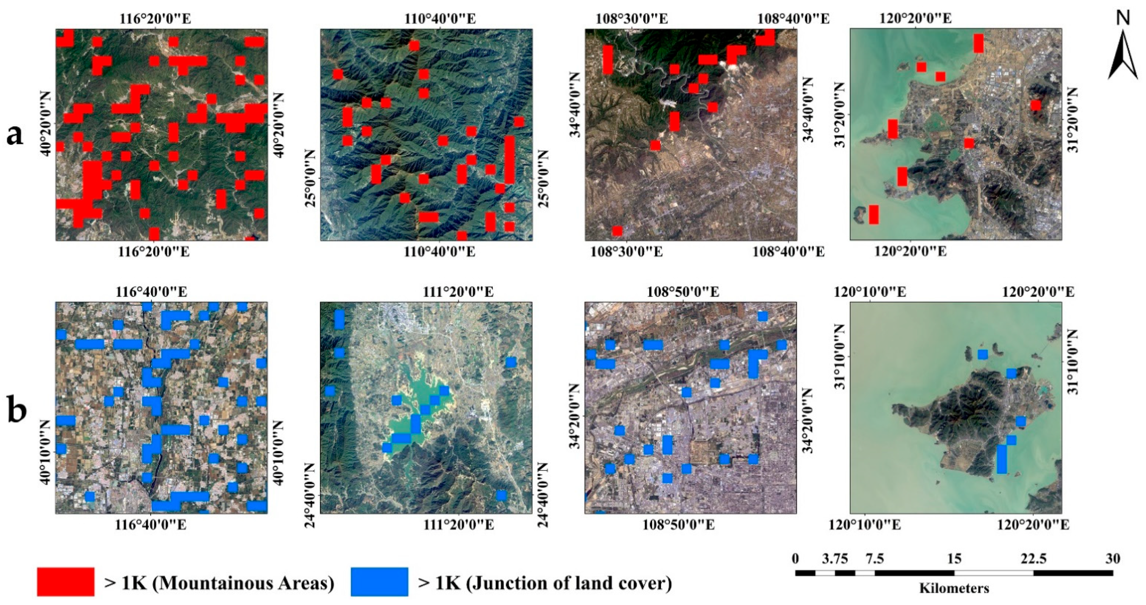
• The inaccuracy of the satellite data itself, the error of the satellite data processing process, and the choice and error of the resampling algorithms will affect the precision of the downscaling results. As the largest residuals source in the verification of downscaling results, areas with major topographic variations and complex land covers have a significant impact on the downscaling results. All of them prove that it is necessary to further optimize and reconstruct the model, and it is also worth paying attention to evaluating the results using ground-based measured LST data;
• With the development of machine learning, machine-learning-based methods have been applied to the study of LST downscaling. The D-DisTrad model proposed in this paper has largely achieved better qualitative and quantitative evaluation results when compared to other linear regression models. A comparison of the downscaling results obtained from the linear regression model-based approach and the machine-learning-based approach for the Sentinel-3 data and the impact factors used in this paper’s model is also well worth the next step, and the results of the comparison may also have implications for how the linear regression model can be improved;
• The SLSTR sensor’s excellent temporal resolution enables it to capture images not only during the day but again at night on the same day. Therefore, two LST data scenes—one for the day and one for the night—can be generated in a single day. If it is considered that the topography and land cover of the study sites are unchanged on the same day, D-DisTrad can also be used to generate nighttime LST downscaling data, which are of great significance and have good prospects for studying the changes in day and night LST data and for related research under long time series.

References

1. Cheval, S.; Dumitrescu, A. The summer surface urban heat island of Bucharest (Romania) retrieved from MODIS images. Theor. Appl. Climatol. 2014, 121, 631–640. [Google Scholar] [CrossRef]
2. Dihkan, M.; Karsli, F.; Guneroglu, A.; Guneroglu, N. Evaluation of surface urban heat island (SUHI) effect on coastal zone: The case of Istanbul Megacity. Ocean Coast Manag. 2015, 118, 309–316. [Google Scholar] [CrossRef]
3. Schwarz, N.; Schlink, U.; Franck, U.; Großmann, K. Relationship of land surface and air temperatures and its implications for quantifying urban heat island indicators—An application for the city of Leipzig (Germany). Ecol. Indic. 2012, 18, 693–704. [Google Scholar] [CrossRef]
4. Feizizadeh, B.; Blaschke, T. Thermal remote sensing for examining the relationship between urban Land surface Temperature and land use/cover in Tabriz city, Iran. In Proceedings of the International Geoscience and Remote Sensing Symposium, Munich, Germany, 22–27 July 2012; IEEE: New York, NY, USA, 2012; pp. 2229–2232. [Google Scholar] [CrossRef]
5. Gazi, M.Y.; Rahman, M.Z.; Uddin, M.M.; Rahman, F.M.A. Spatio-temporal dynamic land cover changes and their impacts on the urban thermal environment in the Chittagong metropolitan area, Bangladesh. GeoJournal 2020, 86, 2119–2134. [Google Scholar] [CrossRef]
6. Maffei, C.; Alfieri, S.M.; Menenti, M. Relating Spatiotemporal Patterns of Forest Fires Burned Area and Duration to Diurnal Land Surface Temperature Anomalies. Remote Sens. 2018, 10, 1777. [Google Scholar] [CrossRef] [Green Version]
7. Maffei, C.; Lindenbergh, R.; Menenti, M. Combining multi-spectral and thermal remote sensing to predict forest fire characteristics. ISPRS J. Photogramm. Remote Sens. 2021, 181, 400–412. [Google Scholar] [CrossRef]
8. Abdullah, H.; Omar, D.K.; Polat, N.; Bilgili, A.V.; Sharef, S.H. A comparison between day and night land surface temperatures using acquired satellite thermal infrared data in a winter wheat field. Remote Sens. Appl. 2020, 19, 100368. [Google Scholar] [CrossRef]
9. Islam, S.; Ma, M. Geospatial Monitoring of Land Surface Temperature Effects on Vegetation Dynamics in the Southeastern Region of Bangladesh from 2001 to 2016. ISPRS Int. J. Geoinf. 2018, 7, 486. [Google Scholar] [CrossRef] [Green Version]
10. Cammalleri, C.; Vogt, J. On the Role of Land Surface Temperature as Proxy of Soil Moisture Status for Drought Monitoring in Europe. Remote Sens. 2015, 7, 16849–16864. [Google Scholar] [CrossRef]
11. Chi, Y.; Sun, J.; Sun, Y.; Liu, S.; Fu, Z. Multi-temporal characterization of land surface temperature and its relationships with normalized difference vegetation index and soil moisture content in the Yellow River Delta, China. Glob. Ecol. Conserv. 2020, 23, e01092. [Google Scholar] [CrossRef]
12. Kalma, J.D.; McVicar, T.R.; McCabe, M.F. Estimating Land Surface Evaporation: A Review of Methods Using Remotely Sensed Surface Temperature Data. Surv. Geophys. 2008, 29, 421–469. [Google Scholar] [CrossRef]
13. Cao, X.; Bao, A.; Li, L. A Study of Retrieval Land Surface Temperature and Evapotranspiration in Response to LUCC Based on Remote Sensing Data in Sanggong River. In Proceedings of the International Conference on Environmental Science and Information Application Technology, Wuhan, China, 4–5 July 2009; pp. 325–329. [Google Scholar] [CrossRef]
14. Kustas, W.P.; Norman, J.M.; Anderson, M.C.; French, A.N. Estimating subpixel surface temperatures and energy fluxes from the vegetation index–radiometric temperature relationship. Remote Sens. Environ. 2003, 85, 429–440. [Google Scholar] [CrossRef]
15. Zhou, D.; Xiao, J.; Bonafoni, S.; Berger, C.; Deilami, K.; Zhou, Y.; Frolking, S.; Yao, R.; Qiao, Z.; Sobrino, J.A. Satellite Remote Sensing of Surface Urban Heat Islands: Progress, Challenges, and Perspectives. Remote Sens. 2019, 11, 48. [Google Scholar] [CrossRef] [Green Version]
16. Chang, Y.; Xiao, J.; Li, X.; Zhou, D.; Wu, Y. Combining GOES-R and ECOSTRESS land surface temperature data to investigate diurnal variations of surface urban heat island. Sci. Total Environ. 2022, 823, 153652. [Google Scholar] [CrossRef]
17. Hulley, G.C.; Gottsche, F.M.; Rivera, G.; Hook, S.J.; Freepartner, R.J.; Martin, M.A.; Cawse-Nicholson, K.; Johnson, W.R. Validation and Quality Assessment of the ECOSTRESS Level-2 Land Surface Temperature and Emissivity Product. IEEE Trans. Geosci. Remote Sens. 2022, 60, 5000523. [Google Scholar] [CrossRef]
18. Zhan, W.; Chen, Y.; Zhou, J.; Wang, J.; Liu, W.; Voogt, J.; Zhu, X.; Quan, J.; Li, J. Disaggregation of remotely sensed land surface temperature: Literature survey, taxonomy, issues, and caveats. Remote Sens. Environ. 2013, 131, 119–139. [Google Scholar] [CrossRef]
19. Li, N.; Wu, H.; Luan, Q. Land surface temperature downscaling in urban area: A case study of Beijing. J. Remote Sens. 2021, 25, 1808–1820. [Google Scholar] [CrossRef]
20. Yoo, C.; Im, J.; Park, S.; Cho, D. Spatial Downscaling of MODIS Land Surface Temperature: Recent Research Trends, Challenges, and Future Directions. Korean J. Remote Sens. 2020, 36, 609–626. [Google Scholar] [CrossRef]
21. Yang, Y.; Cao, C.; Pan, X.; Li, X.; Zhu, X. Downscaling Land Surface Temperature in an Arid Area by Using Multiple Remote Sensing Indices with Random Forest Regression. Remote Sens. 2017, 9, 789. [Google Scholar] [CrossRef] [Green Version]
22. Wang, R.; Gao, W.; Peng, W. Downscale MODIS Land Surface Temperature Based on Three Different Models to Analyze Surface Urban Heat Island: A Case Study of Hangzhou. Remote Sens. 2020, 12, 2134. [Google Scholar] [CrossRef]
23. Feng, G.; Masek, J.; Schwaller, M.; Hall, F. On the blending of the Landsat and MODIS surface reflectance: Predicting daily Landsat surface reflectance. IEEE Trans. Geosci. Remote Sens. 2006, 44, 2207–2218. [Google Scholar] [CrossRef]
24. Zhu, X.; Chen, J.; Gao, F.; Chen, X.; Masek, J.G. An enhanced spatial and temporal adaptive reflectance fusion model for complex heterogeneous regions. Remote Sens. Environ. 2010, 114, 2610–2623. [Google Scholar] [CrossRef]
25. Weng, Q.; Fu, P.; Gao, F. Generating daily land surface temperature at Landsat resolution by fusing Landsat and MODIS data. Remote Sens. Environ. 2014, 145, 55–67. [Google Scholar] [CrossRef]
26. Hutengs, C.; Vohland, M. Downscaling land surface temperatures at regional scales with random forest regression. Remote Sens. Environ 2016, 178, 127–141. [Google Scholar] [CrossRef]
27. Agam, N.; Kustas, W.P.; Anderson, M.C.; Li, F.; Neale, C.M.U. A vegetation index based technique for spatial sharpening of thermal imagery. Remote Sens. Environ. 2007, 107, 545–558. [Google Scholar] [CrossRef]
28. Li, X.; Jiang, T.; Xin, X.; Zhang, H.; Liu, Q. Spatial downscaling of land surface temperature based on MODIS data. Chin. J. Ecol. 2016, 35, 3443–3450. [Google Scholar] [CrossRef]
29. Yang, Y.; Li, X.; Cao, C. Downscaling urban land surface temperature based on multi-scale factor. Sci. Surv. Mapp. 2017, 42, 73–79. [Google Scholar] [CrossRef]
30. Liu, Y.; Zhu, R.; Qian, J.; Dang, C.; Yue, H. Land Surface Temperature Downscaling Based on Multiple Factors. Remote Sens. Inf. 2020, 35, 6–18. [Google Scholar] [CrossRef]
31. Wang, Q.; Atkinson, P.M. Spatio-temporal fusion for daily Sentinel-2 images. Remote Sens. Environ. 2018, 204, 31–42. [Google Scholar] [CrossRef] [Green Version]
32. Rouse, J.W.; Haas, R.H.; Schell, J.A.; Deering, D.W. Monitoring Vegetation Systems in the Great Plains with Erts. In Proceedings of the Third Earth Resources Technology Satellite-1 Symposium, Washington, DC, USA, 10–14 December 1974; p. 309. [Google Scholar]
33. McFEETERS, S.K. The use of the Normalized Difference Water Index (NDWI) in the delineation of open water features. Int. J. Remote Sens. 1996, 17, 1425–1432. [Google Scholar] [CrossRef]
34. Escadafal, R. Remote sensing of arid soil surface color with Landsat thematic mapper. Adv. Space Res. 1989, 9, 159–163. [Google Scholar] [CrossRef]
35. Guo, L.J.; Moore, J.M. Pixel block intensity modulation: Adding spatial detail to TM band 6 thermal imagery. Int. J. Remote Sens. 2010, 19, 2477–2491. [Google Scholar] [CrossRef]
36. Zhao, G.; Xue, H.; Feng, L. Assessment of ASTER GDEM Performance by Comparing with SRTM and ICESat/GLAS Data in Central China. In Proceedings of the 2010 18th International Conference on Geoinformatics, Beijing, China, 18–20 June 2010. [Google Scholar] [CrossRef]
37. Huryna, H.; Cohen, Y.; Karnieli, A.; Panov, N.; Kustas, W.P.; Agam, N. Evaluation of TsHARP Utility for Thermal Sharpening of Sentinel-3 Satellite Images Using Sentinel-2 Visual Imagery. Remote Sens. 2019, 11, 2304. [Google Scholar] [CrossRef] [Green Version]
38. Yang, Y.; Ma, M.; Zhu, X.; Ge, W. Research on spatial characteristics of metropolis development using nighttime light data: NTL based spatial characteristics of Beijing. PLoS ONE 2020, 15, e0242663. [Google Scholar] [CrossRef]
39. Yan, H.; Zhou, G.; Lu, X. Comparative Analysis of Surface Soil Moisture Retrieval Using VSWI and TVDI in Karst Areas. In Proceedings of the International Conference on Intelligent Earth Observing and Applications, Guilin, China, 9 December 2015. [Google Scholar] [CrossRef]
40. Zhu, X.; Helmer, E.H.; Gao, F.; Liu, D.; Chen, J.; Lefsky, M.A. A flexible spatiotemporal method for fusing satellite images with different resolutions. Remote Sens. Environ. 2016, 172, 165–177. [Google Scholar] [CrossRef]
41. Yin, J.; Cai, H.; Tian, P.; Tang, M. Spatial Downscaling Research of the Land Surface Temperature in Karst Region. Geogr. Geoinf. Sci. 2021, 37, 38–46,99. [Google Scholar] [CrossRef]
42. Zhu, L.; Li, J.; Wu, C.; Yang, B.; Li, Q.; Gong, H. Comparison of LST retrieval algorithms between single-channel and split-windows for high-resolution infrared camera. In Proceedings of the 2009 IEEE International Geoscience and Remote Sensing Symposium, Cape Town, South Africa, 12–17 July 2009; pp. I-25–I-28. [Google Scholar] [CrossRef]
43. Wang, X.; Zhong, L.; Ma, Y. Estimation of 30 m land surface temperatures over the entire Tibetan Plateau based on Landsat-7 ETM+ data and machine learning methods. Int. J. Digit. Earth 2022, 15, 1038–1055. [Google Scholar] [CrossRef]
44. Arabi Aliabad, F.; Zare, M.; Ghafarian Malamiri, H. Comparison of the accuracy of daytime land surface temperature retrieval methods using Landsat 8 images in arid regions. Infrared. Phys. Technol. 2021, 115, 103692. [Google Scholar] [CrossRef]
45. Jiménez-Muñoz, J.C.; Sobrino, J.A. A generalized single-channel method for retrieving land surface temperature from remote sensing data. J. Geophys. Res. Atmos. 2003, 108, 4688. [Google Scholar] [CrossRef] [Green Version]
46. Jimenez-Munoz, J.C.; Sobrino, J.A.; Skokovic, D.; Mattar, C.; Cristobal, J. Land Surface Temperature Retrieval Methods From Landsat-8 Thermal Infrared Sensor Data. IEEE Geosci. Remote Sens. Lett. 2014, 11, 1840–1843. [Google Scholar] [CrossRef]
47. Chakraborty, T.C.; Lee, X.; Ermida, S.; Zhan, W. On the land emissivity assumption and Landsat-derived surface urban heat islands: A global analysis. Remote Sens. Environ. 2021, 265, 112682. [Google Scholar] [CrossRef]
48. Qin, Z.; Li, W.; Gao, M.; Zhang, H. Estimation of land surface emissivity for Landsat TM6 and its application to Lingxian Region in north China. In Proceedings of the Conference on Remote Sensing for Environmental Monitoring, GIS Applications, and Geology VI, Stockholm, Sweden, 13–14 September 2006. [Google Scholar] [CrossRef]
49. Song, C.; Jia, L.; Menenti, M. Retrieving High-Resolution Surface Soil Moisture by Downscaling AMSR-E Brightness Temperature Using MODIS LST and NDVI Data. IEEE J. Sel. Top. Appl. Earth Obs. Remote Sens. 2014, 7, 935–942. [Google Scholar] [CrossRef]
50. Sun, D.; Kafatos, M. Note on the NDVI-LST relationship and the use of temperature-related drought indices over North America. Geophys. Res. Lett. 2007, 34, L24406. [Google Scholar] [CrossRef] [Green Version]
51. Wang, S.; Luo, Y.; Li, M.; Yang, K.; Liu, Q.; Li, X. A Taylor Expansion Algorithm for Spatial Downscaling of MODIS Land Surface Temperature. IEEE Trans. Geosci. Remote Sens. 2022, 60, 1–17. [Google Scholar] [CrossRef]
Figure 1. Landsat 8 OLI true color images at 30 m spatial resolution for the study sites: (a) site 1, Beijing; (b) site 2, Guilin; (c) site 3, Xi’an–Xian Yang; (d) site 4, Taihu River Basin.
Remotesensing 14 05752 g001
Figure 2. Data processing flow chart.
Remotesensing 14 05752 g002
Figure 3. Each line goes from left to right, showing the Landsat 8 LST, SLSTR LST, D-DisTrad LST, DisTrad LST, and TsHARP LST data for the 4 study sites: (a) site 1, Beijing; (b) site 2, Guilin; (c) site 3, Xi’an–Xian Yang; (d) site 4, Taihu River Basin. The black box shows the selected areas of noticeable change.
Remotesensing 14 05752 g003
Figure 4. Each line goes from left to right, showing Landsat 8 LST, SLSTR LST, D-DisTrad LST, DisTrad LST, and TsHARP LST data. Areas with noticeable changes for the 4 sites: (a) site 1; (b) site 2; (c) site 3; (d) site 4.
Remotesensing 14 05752 g004
Figure 5. Each line goes from left to right, showing SLSTR LST (900 m), D-DisTrad LST (300 m), DisTrad LST (300 m), and TsHARP LST (300 m) data for site 3 across 4 seasons: (a) winter; (b) spring; (c) summer; (d) fall. The black box shows the selected areas of noticeable change.
Remotesensing 14 05752 g005
Figure 6. Each line goes from left to right, showing SLSTR LST, D-DisTrad LST, DisTrad LST, and TsHARP LST data. Areas with noticeable changes in site 3 across 4 seasons: (a) winter; (b) spring; (c) summer; (d) fall.
Remotesensing 14 05752 g006
Figure 7. Each line goes from left to right, showing SLSTR LST (900 m), D-DisTrad LST (300 m), DisTrad LST (300 m), and TsHARP LST (300 m) data in site 2 across 4 seasons: (a) winter; (b) spring; (c) summer; (d) fall.
Remotesensing 14 05752 g007
Figure 8. Each line goes from left to right, showing SLSTR LST, D-DisTrad LST, DisTrad LST, and TsHARP LST data. Areas with noticeable changes in site 2 across 4 seasons: (a) winter; (b) spring; (c) summer; (d) fall.
Remotesensing 14 05752 g008
Figure 9. Relationship between three downscaling results aggregated to the 900 m resolution and Sentinel-3 SLSTR LST: (a) site 1, Beijing; (b) site 2, Guilin; (c) site 3, Xi’an–Xian Yang; (d) site 4, Taihu River Basin. The solid black line represents the regression line.
Remotesensing 14 05752 g009
Figure 10. The representative areas with errors greater than 1 K in four study sites were selected from site 1 to site 4 from left to right: (a) mountain areas with errors greater than 1 K; (b) junction of land cover types with errors greater than 1 K.
Remotesensing 14 05752 g010