Article

Quantitative Assessment of the Spatial Scale Effects of the Vegetation Phenology in the Qinling Mountains

1
Shaanxi Key Laboratory of Earth Surface System and Environmental Carrying Capacity, Northwest University, Xi’an 710127, China
2
College of Urban and Environmental Science, Northwest University, Xi’an 710127, China
3
Faculty of Geographical Science, Beijing Normal University, Beijing 100875, China
4
Institute of Geomatics, University of Natural Resources and Life Sciences (BOKU), Peter Jordan Strasse 82, 1190 Vienna, Austria
*
Author to whom correspondence should be addressed.
Remote Sens. 2022, 14(22), 5749; https://doi.org/10.3390/rs14225749
Submission received: 17 September 2022 / Revised: 10 November 2022 / Accepted: 11 November 2022 / Published: 14 November 2022
(This article belongs to the Special Issue Remote Sensing in Mountainous Vegetation)

Abstract

:
Vegetation phenology reflects the temporal dynamics of vegetation growth and is an important indicator of climate change. However, differences consistently exist in land surface phenology derived at different spatial scales, which hinders the understanding of phenological events and integration of land surface phenology products from different scales. The Qinling Mountains are a climatic and geographical transitional region in China. To better understand the spatial scale effect issues of land surface phenology in mountainous ecosystems, this study up-scaled vegetation start of season (SOS) and end of season (EOS) in the Qinling Mountains derived from three different Moderate Resolution Imaging Spectroradiometer (MODIS) normalized difference vegetation index (NDVI) products to four scales (i.e., 2 km × 2 km, 4 km × 4 km, 6 km × 6 km, and 8 km × 8 km) using the spatial averaging method. Then, similarities and differences between the up-scaled SOSs/EOSs were examined using the simple linear regression, cumulative distribution function, and absolute difference. Finally, the random forest model was used to reveal the major factors influencing the spatial scale effect of land surface phenology in Qinling Mountains. Results showed that the derived basic SOS/EOS datasets using the same filtering method from the 250 m and 500 m NDVI datasets were consistent in spatial distribution, while the results from the 1000 m NDVI dataset differed. For both the basic and the up-scaled datasets, the land surface phenology derived from the Savitzky-Golay-filtered NDVI showed an advance in SOS, but a delay in EOS, compared to those derived from the asymmetric Gaussian- and double logistic-filtered NDVI. The up-scaled SOS was greatly impacted by both NDVI resolution and the filtering methods. On the other hand, EOS was mostly impacted by the filtering methods. Moreover, up-scaled SOSs usually had larger differences compared to up-scaled EOSs. While different filtering methods sometimes amplified the absolute differences between different SOS/EOS across scales, the upscaling reduced the differences. Influence factor analysis showed that spatial variations observed in SOS in Qinling Mountains were mainly caused by forest cover, uneven distribution of spring precipitation, and annual precipitation, while spatial variations in aspect, winter temperature, and autumn precipitation all strongly influenced the observed EOS across scales in the study area. These findings enhance our understanding of the effects of observational scale on vegetation phenology in mountain ecosystems and provide a reference for phenology modeling in mountainous areas.

Graphical Abstract

1. Introduction

Vegetation phenology involves several important cyclical plant phenomena, such as germination, leaf development, flowering, and defoliation [1,2]. These phenological processes can reflect the differences in species interactions and ecosystem functions and are impacted by climate change. Satellite-derived phenology is termed as land surface phenology (LSP), which quantifies seasonal dynamics of vegetation activity [3]. Rapid progress in remote sensing technologies have greatly expanded the scope of phenological studies, thereby improving our understanding of land surface phenology from local to global scales [4,5]. Due to its periodic/recurrent nature and sensitivity to climate change, land surface phenology is considered an important vegetation indicator [6,7]. Additionally, land surface phenology provides suitable references for studying global climate change, biodiversity changes, ecosystem structure alterations [8,9,10], and carbon budget dynamics [11]. Land surface phenology metrics are also widely used in remote sensing-based drought monitoring systems [12] and for yield forecasting purposes [13].
During the last two decades, many land surface phenology products that developed using different satellite data have assisted in capturing variations in global vegetation phenology [14,15,16,17,18,19] and supporting the related research [20,21,22,23]. However, several studies have revealed that the results of phenology products derived from different data sources are inconsistent [24,25], with some differences being too large to ensure suitable comparison [26]. Observed differences can be caused by differences in various factors, such as the selected vegetation index (VI) [6,27], spectral settings of satellites [7], radiometric resolution of sensor bands [17,28], and spatiotemporal resolution of different datasets [29,30]. Among these, spatial resolution is believed to be the most significant factor responsible for the observed discrepancies between different phenology products [5]. Phenological discrepancies have also been recognized as being scale-dependent because the ecological patterns vary spatially [31].
The impact of noises in the VI time series cannot be neglected when VIs are used to retrieve vegetation phenology [21,27,28]. As optical data are negatively affected by clouds and poor atmospheric conditions, different filtering and smoothing techniques have been developed, which add to the observed differences in the subsequently derived land surface phenology products (e.g., Atkinson et al. [32]). The problem is further amplified by the fact that hectometric to kilometric scale products are notoriously difficult to validate via field measurements [26]. To circumvent this problem, either comparative studies can be performed or assessments of the product’s usefulness in downstream applications is needed [33].
To quantitatively analyze the phenological differences derived at different scales, several studies have scaled up fine-resolution phenology and compared it with the coarse-resolution phenology [34,35,36]. For example, Fisher and Mustard [37] calculated the average of 30 m Landsat-5 start of season (SOS) results at 500 m and then compared it with the average of the 500 m Moderate Resolution Imaging Spectroradiometer (MODIS) SOS results. Their results showed a difference of approximately 0–25 days in SOS, with no systematic bias. Delbart et al. [38] verified the green-up dates of four woody plants in Canada obtained from SPOT-VEGETATION by calculating the average value of ground-observed SOS, and found that the difference was 13.6–15.6 days. Peng et al. [3] investigated the vegetation SOS in the continental United States by resampling 250 m MODIS enhanced vegetation index (EVI) to different spatial resolutions (250 m, 2 × 250 m, 3 × 250 m, …, 35 × 250 m) and reported that SOS changed linearly or logistically when EVI became coarser. Among the six ecological regions analyzed, five showed increases in SOS when EVI became coarser (that is, green-up was delayed). Contrastingly, Zhang et al. [34], who studied maize and soybean planting areas in the United States, reported that the 500 m green-up dates were advanced compared to the 30 m green-up dates.
Although other studies investigated the observational scale effects of remotely sensed vegetation phenology for different vegetation types, most studies focused on only two scales, with few considering multiple-scale analysis. Additionally, autumn phenology has rarely been studied, and different studies have provided contrasting conclusions concerning phenology products or pre-processing. Together, the mentioned gaps and discrepancies illustrate the complexity of the spatial scale effects of remotely sensed phenology. To address this research gap, studies on scale effects in different regions and vegetation ecosystems are required to better understand these issues and integrate different phenology products.
Qinling Mountains are a crucial ecological conservation area and geographical and climatic transition zone in China. This provides an ideal area for examining land surface phenology spatial scale issues in a mountainous region. Accordingly, this study aimed to quantitatively demonstrate the changes in vegetation phenology in the Qinling Mountains derived from different up-scaled data sources. Initially, we acquired three MODIS normalized difference vegetation index (NDVI) products, and then smoothed the three NDVI time series using the three filters to retrieve the vegetation SOS and end of season (EOS). Subsequently, the datasets were up-scaled to 2 km × 2 km, 4 km × 4 km, 6 km × 6 km, and 8 km × 8 km resolutions using spatial averaging. The cumulative distribution function (CDF), the absolute difference, and the linear regression methods were utilized to measure the differences between the up-scaled SOSs/EOSs. Finally, we also investigated the major influencing factors that impacted the spatial scale effects of local land surface phenology.

2. Materials and Methods
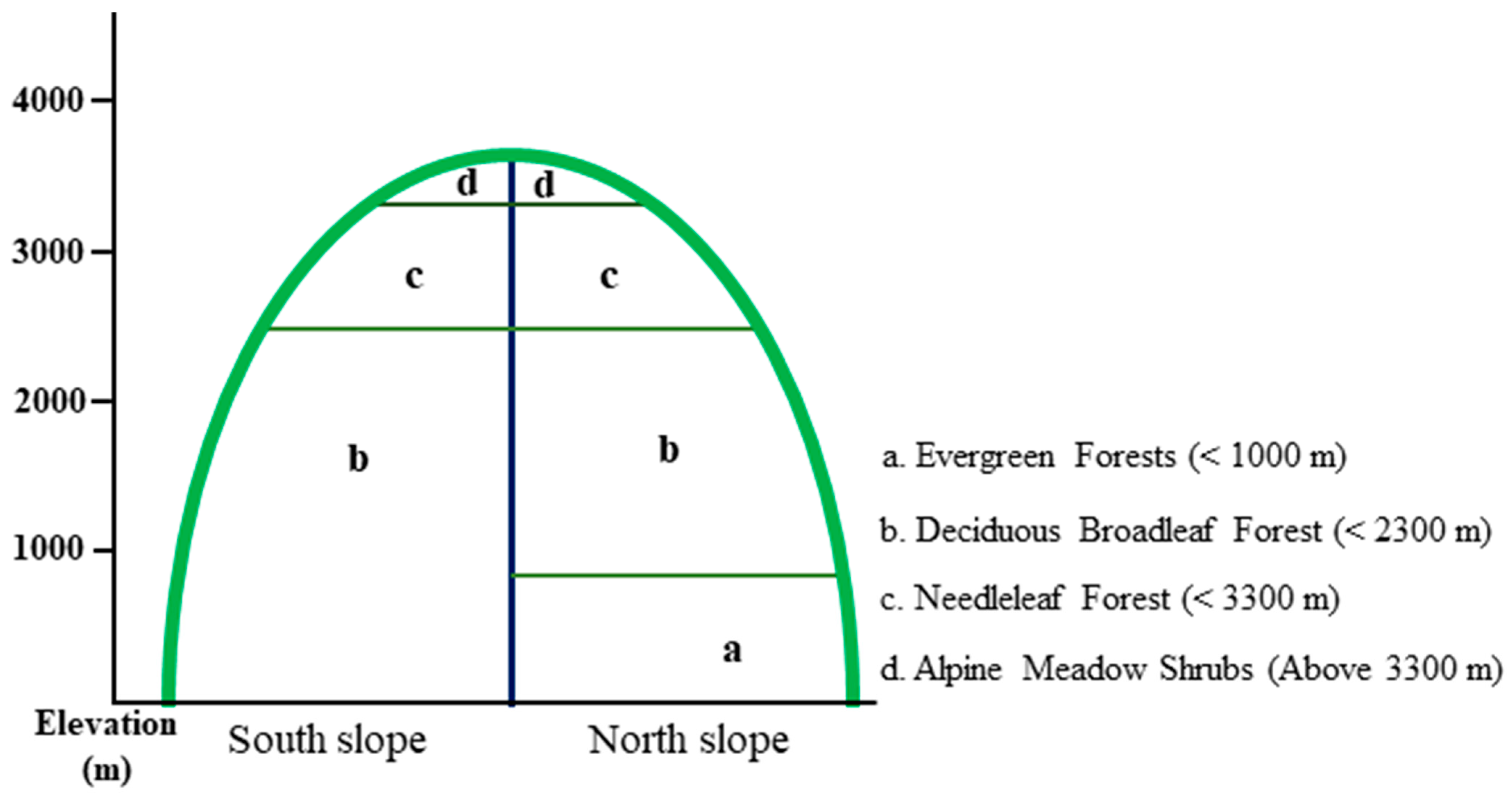
2.1. Study Area

Our specific study area is confined to the parts of the Qinling Mountains within Shaanxi Province, China [39]. This region ranges from 105°30′E to 111°05′E, and from 31°40′N to 34°35′N (Figure 1). It is located in the southern part of Shaanxi Province, south of the Weihe River and north of the Hanjiang River. The total acreage is 61,900 km2, which accounts for 30% of the total area of Shaanxi Province, China. The altitude range is 171–3747 m [40]. The Qinling Mountains can be divided into the north and south slopes by the Qinling mountain line [40,41]. Since we focus on the SOS and EOS changes of mountainous vegetation, Hanzhong Basin was excluded from further analysis as it is mainly used for crop plantations.
Qinling Mountains represent a climatic and geographic transition zone between south and north China [36], and between warm temperate and subtropical climates. Moreover, China’s 0° isotherm passes through this region. As a result, large-scale differences in climate (Figure 2a,b), plants [42,43], soil, and agricultural land use exist between north and south regions of the Qinling Mountains [10,44]. Specifically, the climate is dry in the north and wet in the south. In addition, the elevation gradually increases from east to west and the topography of Qinling Mountains is characterized by mountains and hills [45] (Figure 2c). Slightly acid yellow-brown soil developed from granitic gneiss dominates in the south, while calcareous soil dominates in the north [40]. The forest cover of the study area exceeds 70%, and its distribution of vegetation types also presents an obvious transition from the north to the south (Figure 2d) [46], with the north slope dominated by warm temperate deciduous broad-leaved forests and the south slope characterized by deciduous broad-leaved forests mixed with evergreen species [28]. Further, from the north to the south of the Qinling Mountains, evergreen forests occur at lower elevations, while the larch forest belt is distributed across higher elevations (Figure 3) [46]. These differences in the vegetation types lead to spatiotemporal diversity in vegetation phenology and growth status on the north and south slopes.

2.2. Data Sources and Pre-Processing

(1) MODIS NDVI data. To explore the scale effects of land surface phenology, three MODIS NDVI datasets were considered in this study, including MOD13Q1, MOD13A1, and MOD13A2, with spatial resolutions of 250 m, 500 m, and 1000 m, respectively. The three datasets have the same temporal resolution (16 days) [47,48]. Thus, temporal sampling effects could be ignored in this study. The data during 2017–2019 were obtained from the United States Geological Survey (https://lpdaacsvc.cr.usgs.gov/ (accessed on 12 September 2020)) for retrieving vegetation SOS and EOS in 2018. The atmospheric contamination has already been considered during the production of the three datasets.
(2) Meteorological data. To investigate the impacts of precipitation and temperature on the spatial scale effects of land surface phenology, we also downloaded the 1 km monthly precipitation [49,50,51,52,53] and temperature [49,54,55,56] datasets in 2017–2018 from the National Tibetan Plateau Data Center (http://data.tpdc.ac.cn/ (accessed on 19 July 2022)). Based on the two datasets, yearly average temperature (Figure 2a) and yearly total precipitation (Figure 2b) can be calculated. However, studies have revealed that vegetation phenology in this region is mainly driven by seasonal meteorological conditions rather than yearly conditions [40,44]. Therefore, we also calculated the seasonal total precipitation and average temperature. Seasons are divided into three months per season with the start in January.
(3) Topographic data. Since the study area is in a mountainous region, the influence of topographic conditions cannot be neglected. The 12.5 m Advanced Land Observing Satellite (ALOS) Digital Elevation Model (DEM) data (Figure 2c) were downloaded from the National Aeronautics and Space Administration (https://search.asf.alaska.edu/#/ (accessed on 7 January 2021)) [57], the slope and aspect are calculated based on the DEM data.
(4) Land cover data. The composite and structure of tree species are highly related to the dynamics of vegetation phenology in Qinling Mountains. However, an accurate map of tree species in the study area is unavailable. As a supplement, a high spatial resolution land cover map can provide complementary information about the ground surface cover. This study obtained the 30 m GlobeLand30 land cover map in 2020 (http://www.globallandcover.com/ (accessed on 15 July 2022)) for characterizing the tree cover status in this region [41] (Figure 2d).

2.3. Method

Vegetation phenology (SOS and EOS) was first retrieved from differently processed NDVI datasets at 250 m, 500 m, and 1000 m. Afterwards, the basic SOS/EOS datasets were up-scaled to the four desired spatial scales using spatial averaging (Figure 4). Simple linear regression was used to examine the similarities and differences between the up-scaled SOSs and EOSs at different scales. To show the spatial scale effects caused by spatial resolution and the filtering methods, cumulative distribution functions (CDF) of each up-scaled SOS/EOS were derived as well as the absolute difference between the up-scaled SOSs/EOSs. Finally, the random forest model was used to reveal the major factors that influencing the spatial scale effect of SOS/EOS in the study area.

2.3.1. Retrieval of SOS and EOS

We used TIMESAT 3.3 software to obtain the basic vegetation SOS and EOS from the NDVI time series using three data smoothing and fitting functions: the asymmetric Gaussian (AG) filter [58], the double logistic (DL) filter [59], and the Savitzky-Golay (SG) filter [60]. These three methods are extensively used in vegetation phenology research to pre-process and analyze vegetation index time series contaminated by clouds and atmospheric conditions. To focus on scale effects, other prominent filters, such as the Whittaker smoother [16] and harmonic analysis [59], were not included.
Vegetation activity follows a strong seasonal cycle. NDVI curves can thus be fitted using simple Gaussian functions [58]. However, due to factors such as vegetation type, topography, temperature and precipitation pattern, vegetation NDVI often cannot be fitted perfectly with a standard Gaussian curve [61]. The asymmetric Gaussian and double logistic filter can better capture the asymmetry in the NDVI curves with generally consistent results [59]. Unlike the asymmetric Gaussian and the double logistic filter, the Savitzky-Golay (SG) filter is based on temporally localized least squares-fits [62], which smooths the (noisy) observations in overlapping temporal windows to remove noise in the time series data [27].
To retrieve the land surface phenological metrics of any target year (here 2018), the TIMESAT software requires input of three consecutive and encompassing years of NDVI data. We used 2017–2019 NDVI to obtain vegetation SOS and EOS in 2018. To minimize the impact of different parameter settings, parameters were set to standard settings for all three filters (Table 1). The only difference is that when the Savitzky-Golay (SG) filter was used, there was a specific parameter—window size. The window size was set as two, representing 32 days in this study. Then, for SOS and EOS retrieval, as only one season occurs per year in the study region, the seasonal parameter was set as one. The seasonal amplitude method was used to retrieve SOS/EOS for all conditions [63]. Both SOS and EOS retrieval values were set as 0.2 of the full amplitude. Obviously, all parameter settings have the potential to impact the retrieved vegetation phenology.

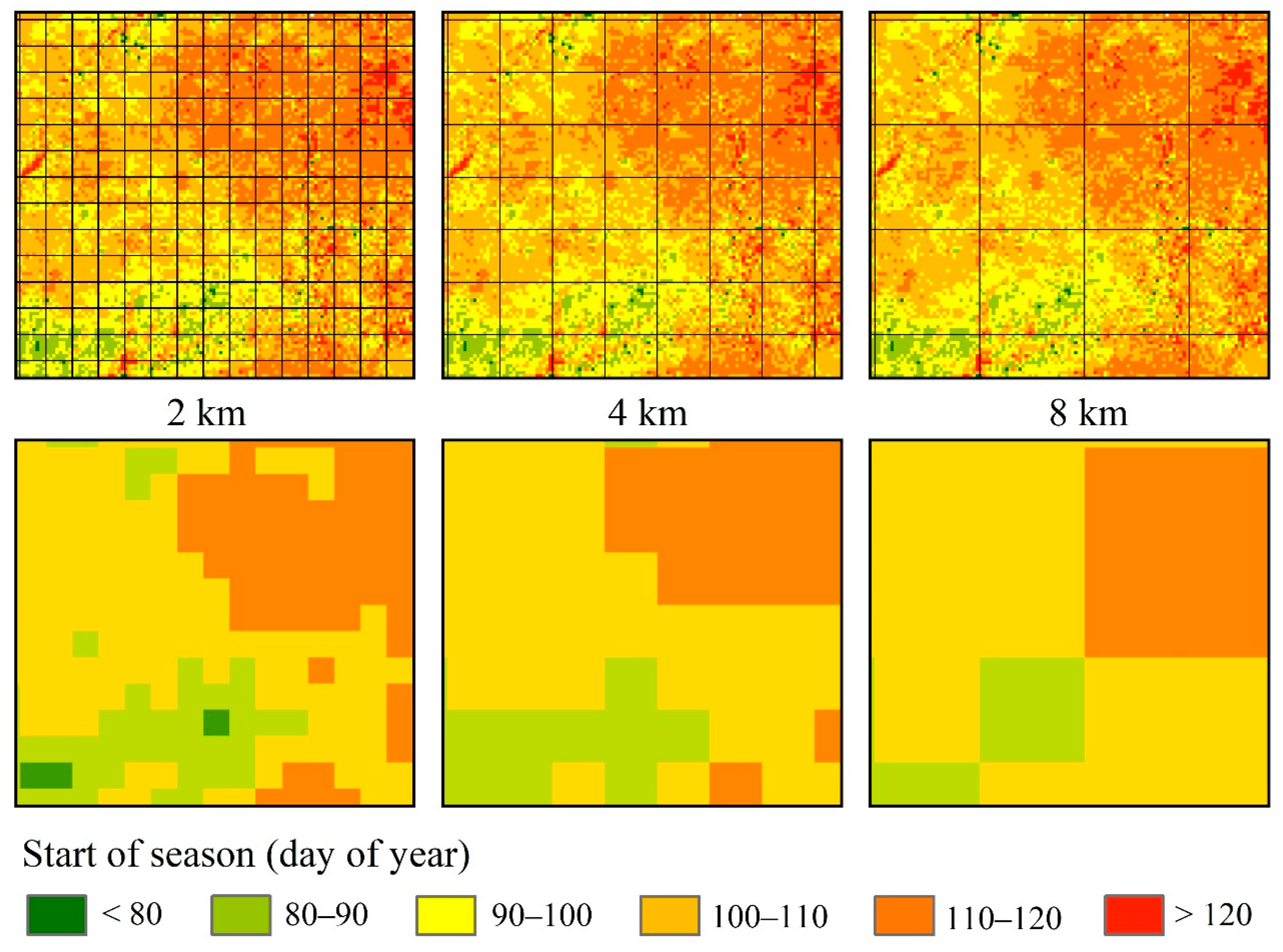
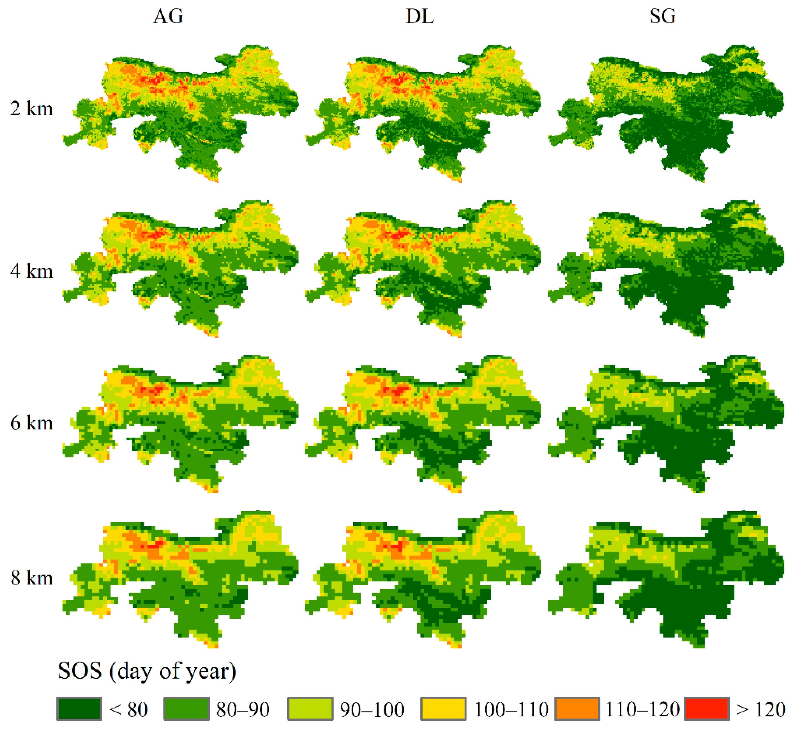
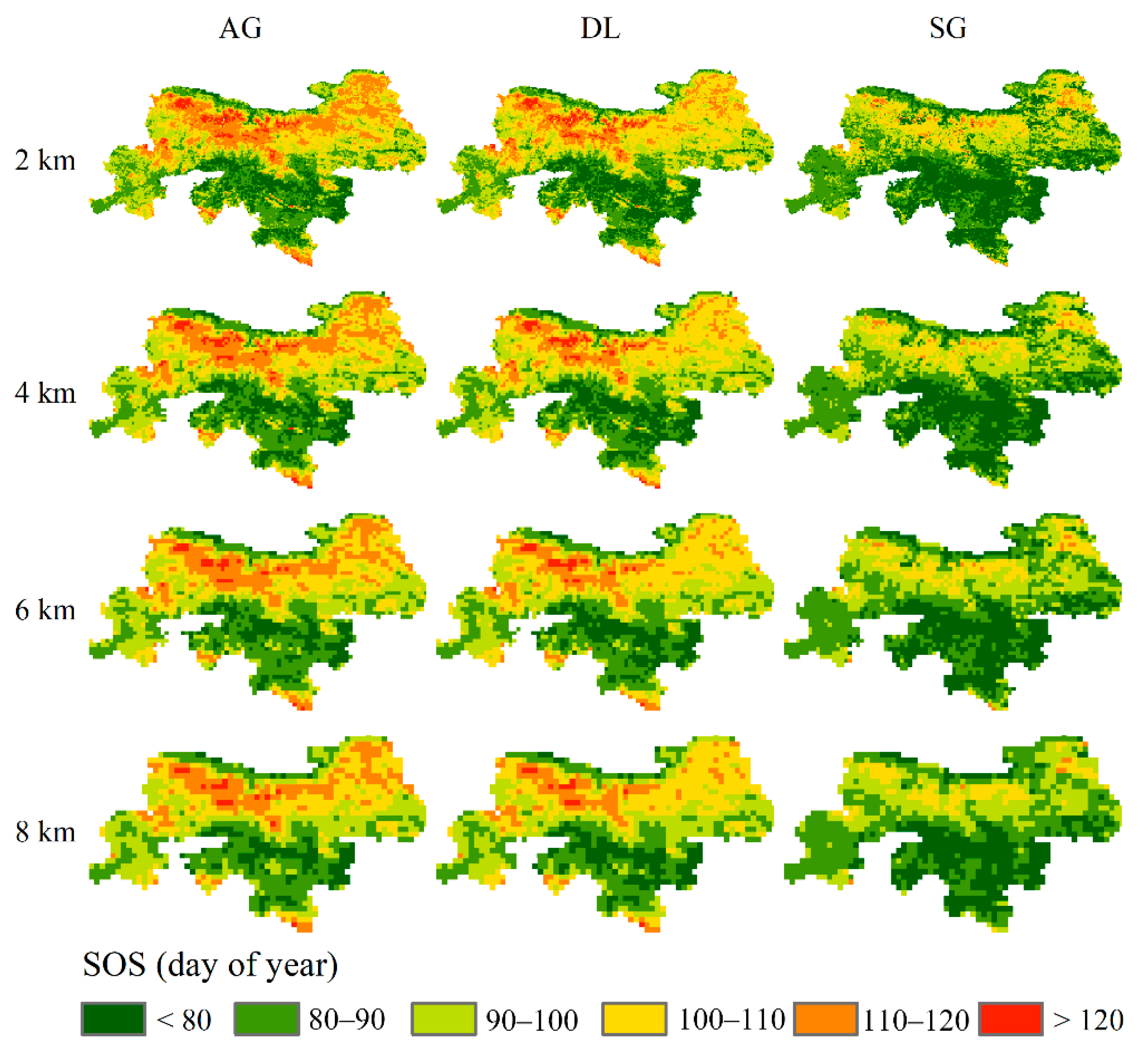
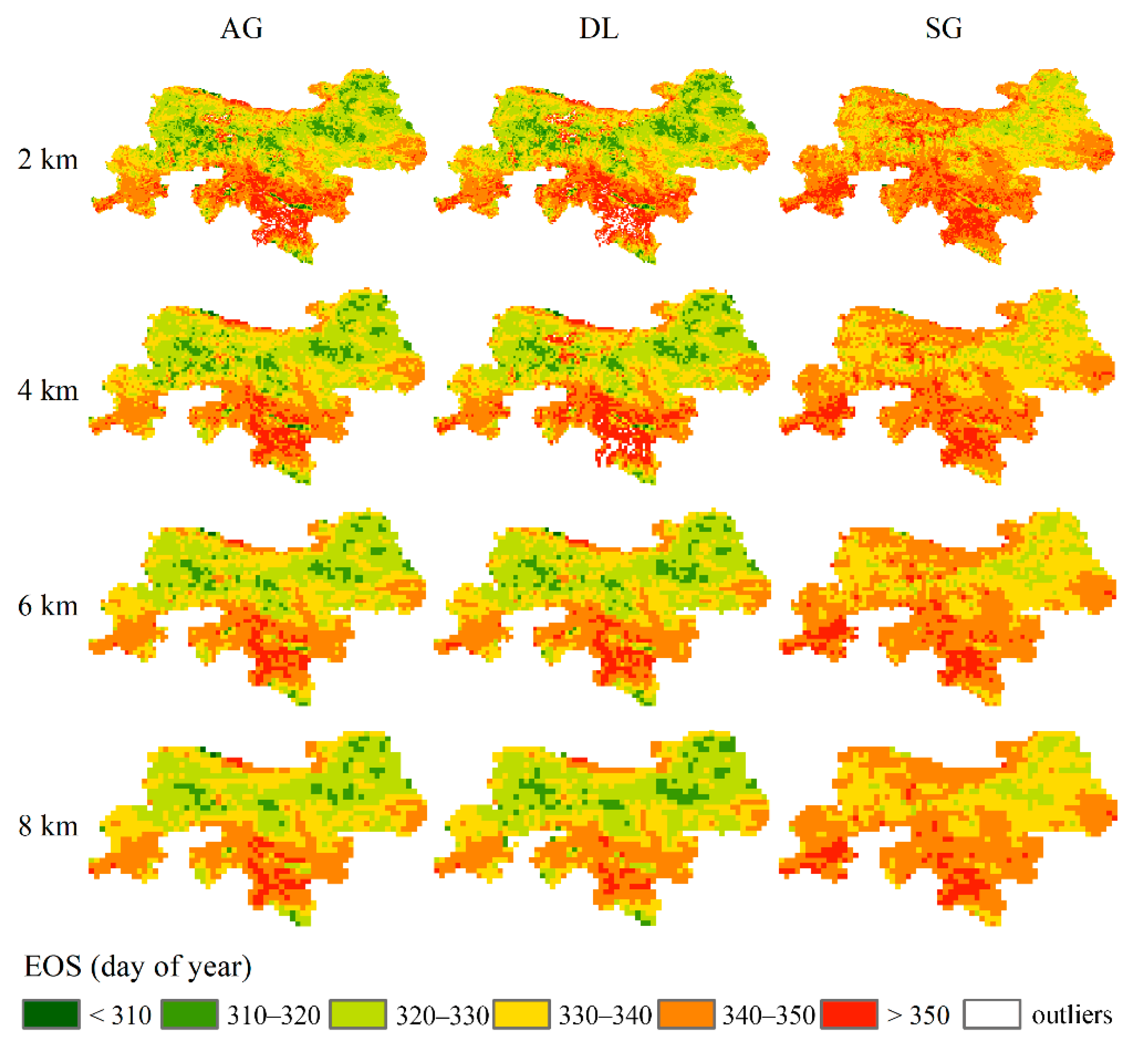
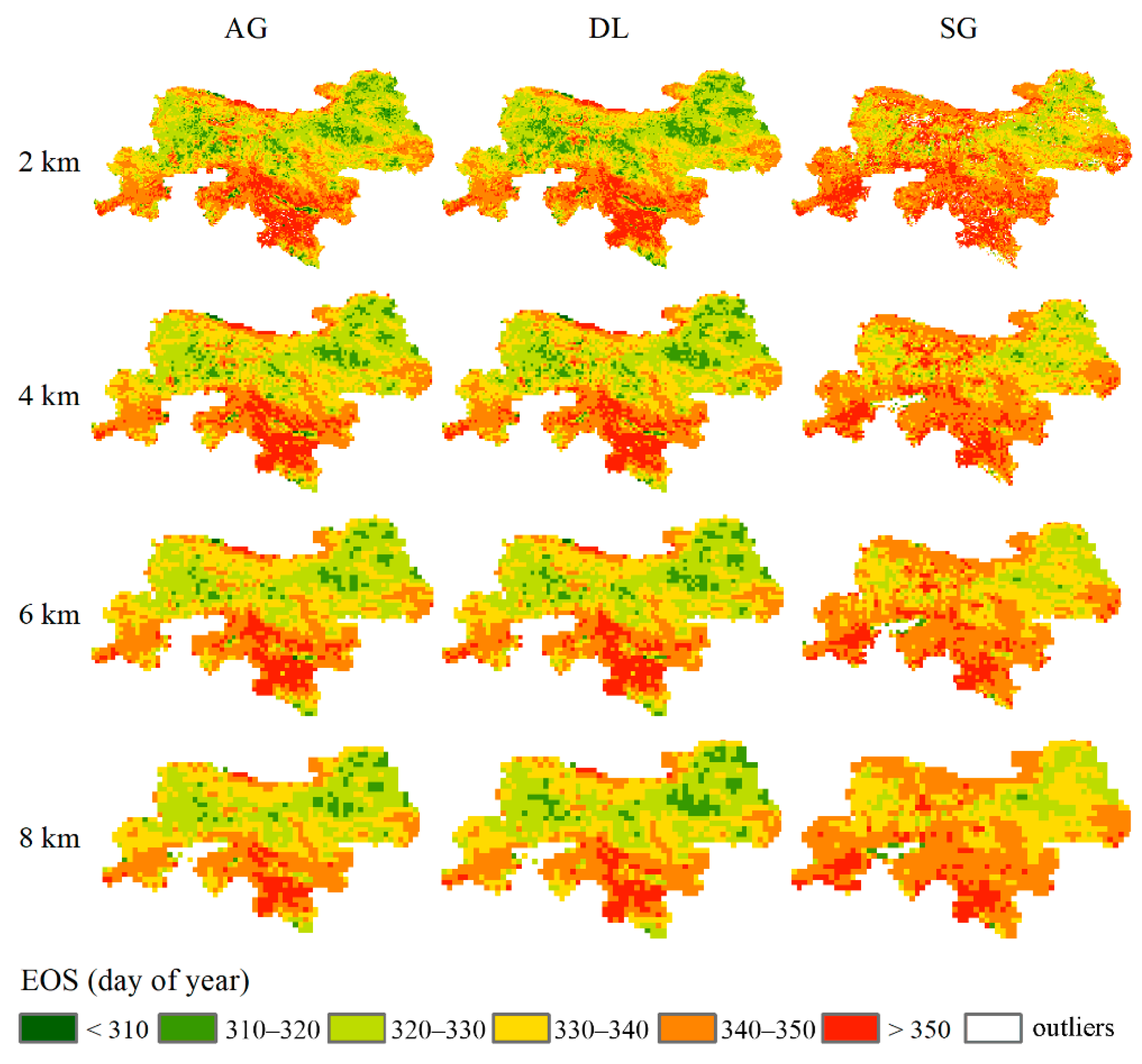
2.3.2. Upscaling of SOS and EOS

Differences in vegetation phenology retrieved from NDVI data of different spatial resolutions should be unified to the same scale for suitable comparison. This can be achieved by upscaling the phenology metrics retrieved from finer resolution remote sensing data and then comparing them with the phenology metrics retrieved from coarser resolution remote sensing data. The spatial averaging method [5,64] and the percentile aggregation method [34,35] are commonly used upscaling methods in phenology studies. The former calculates the mean values of fine-resolution vegetation phenology metrics within the corresponding areas of the coarse-resolution pixels [38]. The latter calculates the cumulative percentage of fine-resolution vegetation phenology in ascending order and determines the cumulative percentage of fine-resolution phenology corresponding to the coarse resolution at the same spatial location [34]. By comparing different upscaling methods, several studies indicated that the averaging approach can be sufficiently employed in most studies [5,65]. The averaging method was thus selected to obtain the up-scaled vegetation SOS/EOS in this study.
The upscaling process is illustrated in Figure 4. First, we created a series of grids with different size (i.e., 2 km × 2 km, 4 km × 4 km, 6 km × 6 km, and 8 km × 8 km) covering the basic SOS/EOS data (Figure 5). Any grid cells not fully in the study area were removed. After that, we calculated the average SOS/EOS within each grid at each scale. Background pixels and outliers (missing values) were set as no-data and ignored during the calculations. This ensures that border grid cells are not influenced by the background.

2.3.3. Quantitative Analysis of the Spatial Scale Effect

After upscaling, we carried out the linear regression to measure the similarities and differences between the up-scaled SOSs or EOSs at each scale and the coefficient of determination (R2) between two up-scaled SOSs or EOSs was derived [66]. The closer R2 is to one, the closer the two up-scaled SOSs or EOSs are. Also, the root mean square error (RMSE) [67] between two up-scaled SOSs or EOSs was calculated. A lower RMSE indicates the two up-scaled SOSs or EOSs are close to each other. The equation for calculating RMSE is as follow:
R M S E = i = 1 m ( X i Y i ) 2 m
where X represents one up-scaled SOS or EOS, and Y denotes another up-scaled SOS or EOS at the same scale as X, m is the number of grids at this scale.
The cumulative distribution functions (CDF) were also calculated to show the value distribution difference of the up-scaled SOS and EOS datasets. To further highlight differences between the various results, we calculated the absolute difference between the up-scaled results at each scale. We mainly considered two circumstances:
  • Up-scaled SOSs/EOSs from the same filtering method but from different input data sets (e.g., from different spatial resolutions).
  • Up-scaled SOSs/EOSs from different filtering methods and different spatial resolutions.
For (1) we calculated the absolute difference between the up-scaled SOS/EOS of the 250 m and 1000 m SOS based on the AG-filtered NDVI, and for (2) we calculated the absolute difference between the 250 m SOS/EOS obtained through SG-filtering and the 1000 m SOS/EOS obtained through AG-filtering, and these results are representative for other combinations. For both circumstances, the absolute differences were calculated, and then the corresponding values of the 20%, 40%, 60%, and 80% cumulative frequency of the 2 km SOS/EOS difference were taken as the breaking points. The absolute differences at other spatial scales were separated at these breaking points to show the changes in the up-scaled SOS/EOS as the spatial resolution becomes coarser.

2.3.4. Investigation of the Factors Influencing the Spatial Scale Effects of Land Surface Phenology

Land surface phenology spatial scale effects are measured by the difference of the maximum SOS (EOS) and the minimum SOS (EOS) in each grid at the four scales. In order to exclude the impacts of filtering methods, we only considered SOS/EOS derived from the same filtering method. To be more specific, we calculated SOS spatial scale effect by using the SOS derived from the 250 m AG-filtered NDVI minus that derived from the 1000 m AG-filtered NDVI at all four scales. Similarly, EOS spatial scale effect was computed by using the EOS derived from the 250 m AG-filtered NDVI minus that derived from the 1000 m AG-filtered NDVI at all four scales. Thus, the spatial scale effect of SOS/EOS can show how big the differences are between the observed SOS/EOS across scales.
Local geographic and environmental conditions strongly influence vegetation phenology. Several studies in this region confirm that meteorological factors are the main factors affecting the long-term variations in SOS and EOS in Qinling Mountains [68,69,70]. In addition, topography strongly impacts vegetation phenology [71]. Moreover, vegetation phenology is directly related to the surface vegetation types, coverage, composite, and structure. Therefore, we considered meteorological, topographic, and forest cover factors (Table 2) in investigating the factors influencing the spatial scale effects of land surface phenology.
The grid difference of each factor directly shows the uneven distribution of this factor in a grid or reflects the heterogeneity of this factor in a grid. Since these factors are different in units and data ranges, the random forest (RF) model [72] was utilized in this study to detect the major influencing factors because it is a nonparametric multivariate method and has no requirements for statistical assumptions [73,74]. It can handle complex relationships with high efficiency, as well as to determine the relative importance of each input feature [70,75]. The relationships between LSP spatial scale effect and the considered meteorological, topographic, and forest cover factors may be non-linear and complex, thus, we detected the relatively significant influencing factors using the important analysis of the RF model.

3. Results

3.1. Qualitative Comparison of the Derived SOS and EOS

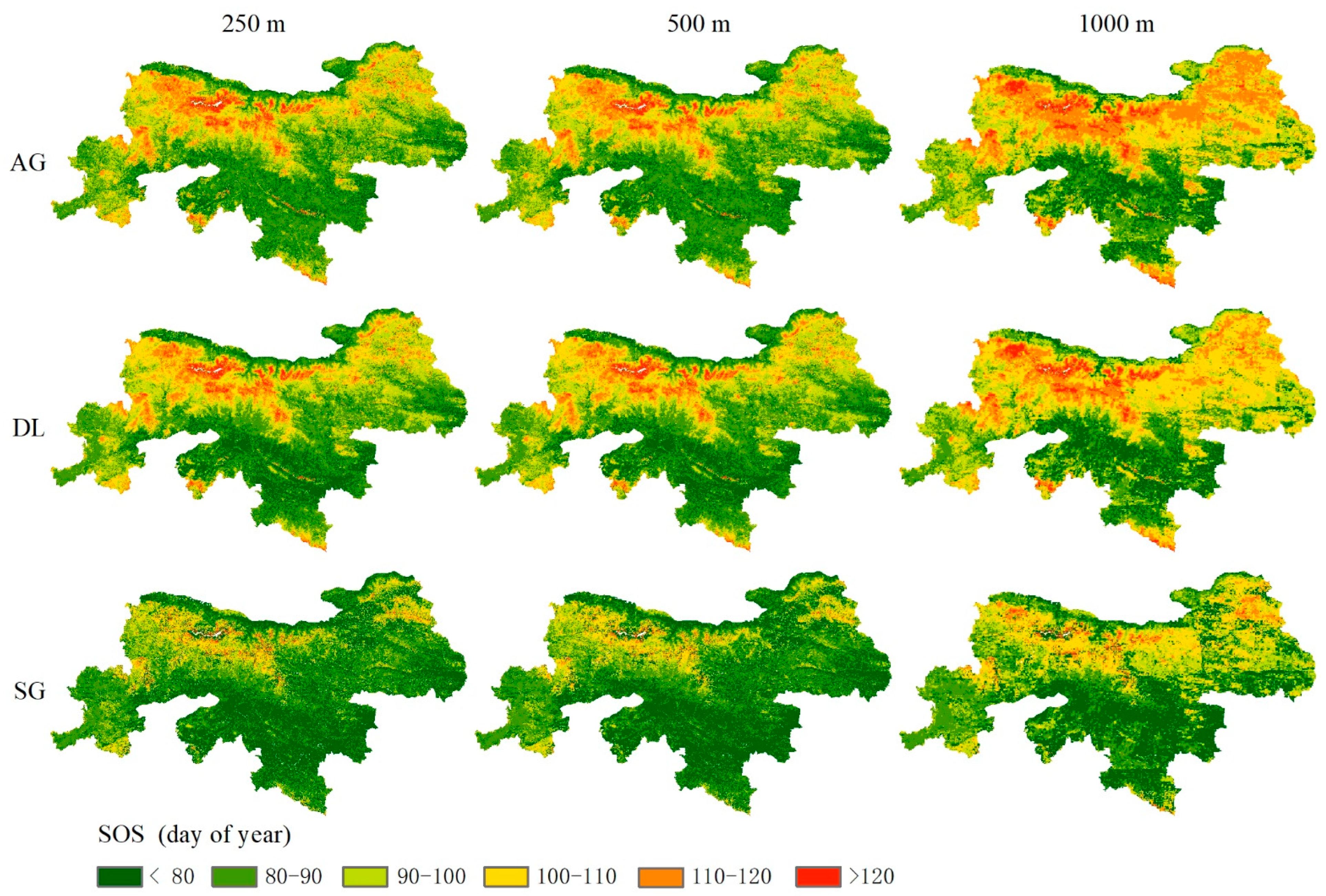
3.1.1. Spatial Distribution of SOS from Three NDVI Datasets at 250 m to 1 km

The maps of vegetation SOS derived from the three NDVI datasets are shown in Figure 6. Each row presents SOS retrieved from the three spatial resolutions (e.g., 250 m, 500 m, and 1 km) using the same smoothing method. Compared with the SOS retrieved from the 250 m and 500 m NDVI datasets, the SOS retrieved from the 1000 m NDVI dataset was significantly delayed in the ridge region but advanced on both sides of the ridge. The SOS spatial distribution obtained from the AG-filtered and DL-filtered NDVI were almost the same, but the SOS obtained by SG-filtering was biased to earlier dates (by approximately 10 days).

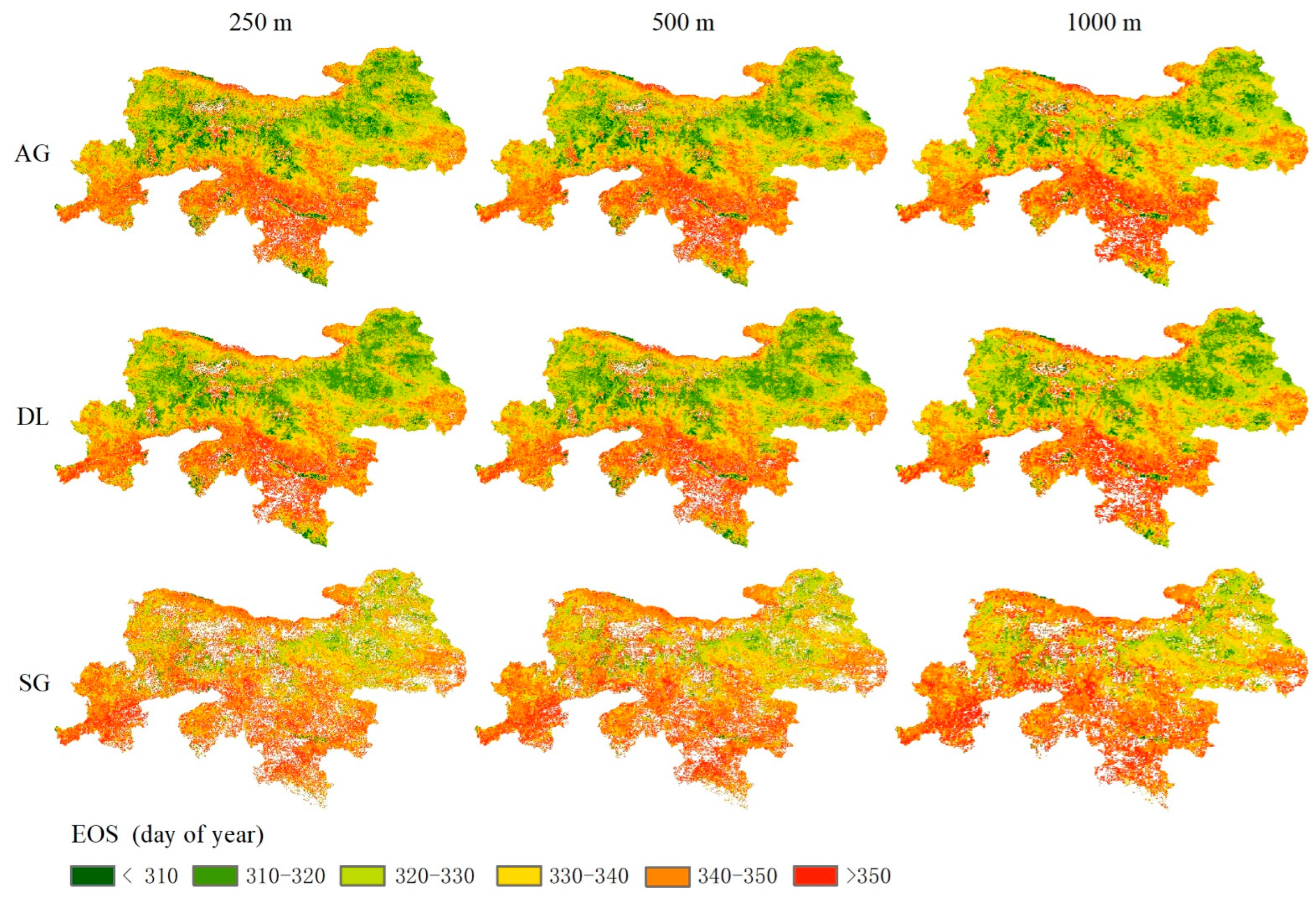
3.1.2. Spatial Distribution of Vegetation EOS from Three NDVI Datasets at 250 m to 1 km

The EOS maps derived from the three NDVI datasets are shown in Figure 7. The blank areas in the figure represent masked-out anomalous EOS data; they had been flagged as missing values in the TIMESAT output result. In the results acquired through AG- and DL-filtering, fewer outliers were found compared to the SG-filtering. Outliers were mainly located on the ridge and in the south sloping areas. All outliers were excluded to ensure accuracy of the subsequent analysis.
The distributions of EOS based on the datasets filtered by the same filtering method (each row) were consistent with each other. Compared with the EOS data derived from the 250 m and 500 m datasets, EOS data from the 1000 m dataset indicated that vegetation green-up occurred earlier in the ridge area and relatively later on the south and north slopes. Compared to EOS data retrieved through AG- and DL-filtering, those retrieved by SG-filtering were delayed, especially in the south and north sloping areas.

3.2. Quantitative Comparisons of the Up-Scaled SOSs and EOSs

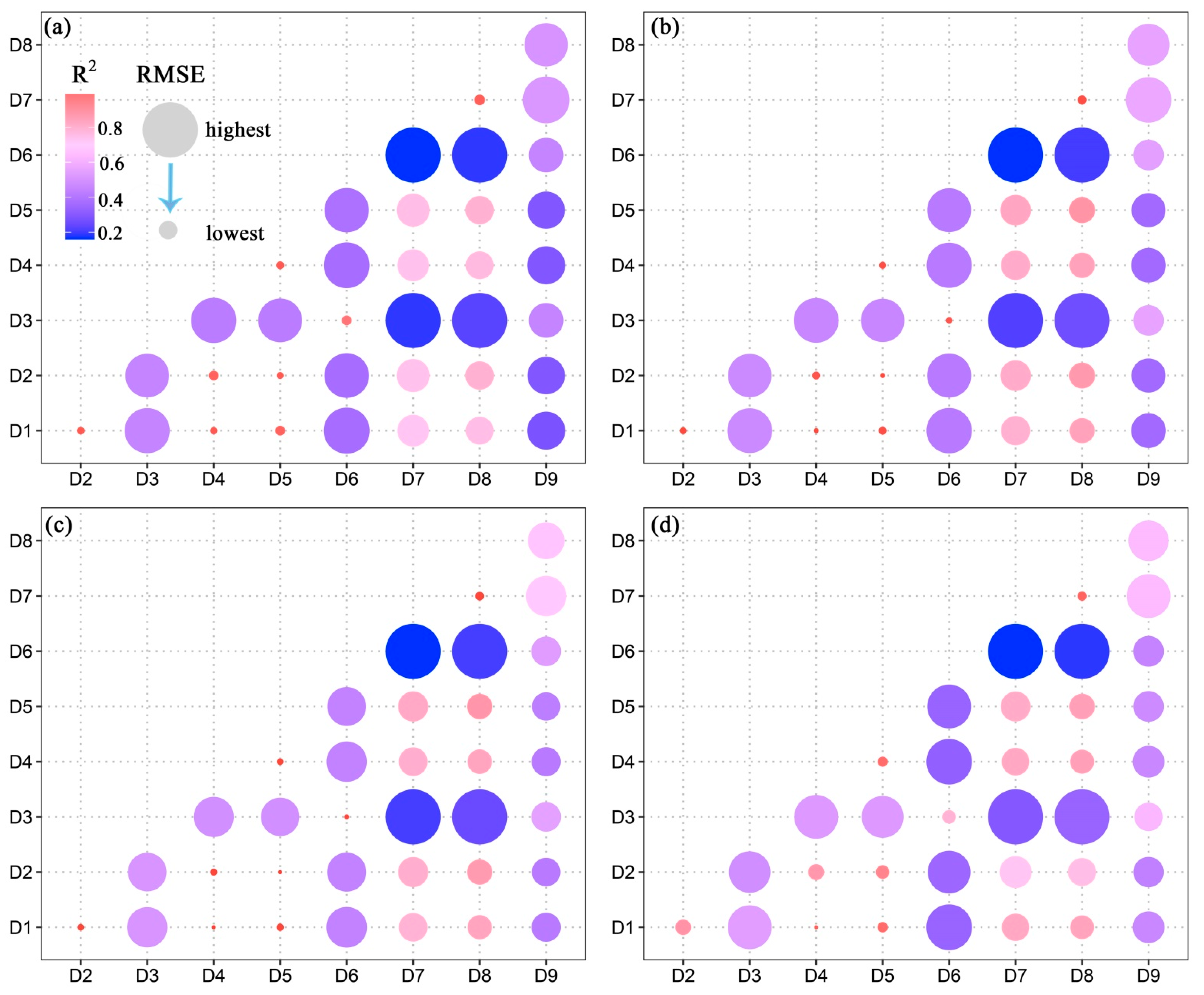
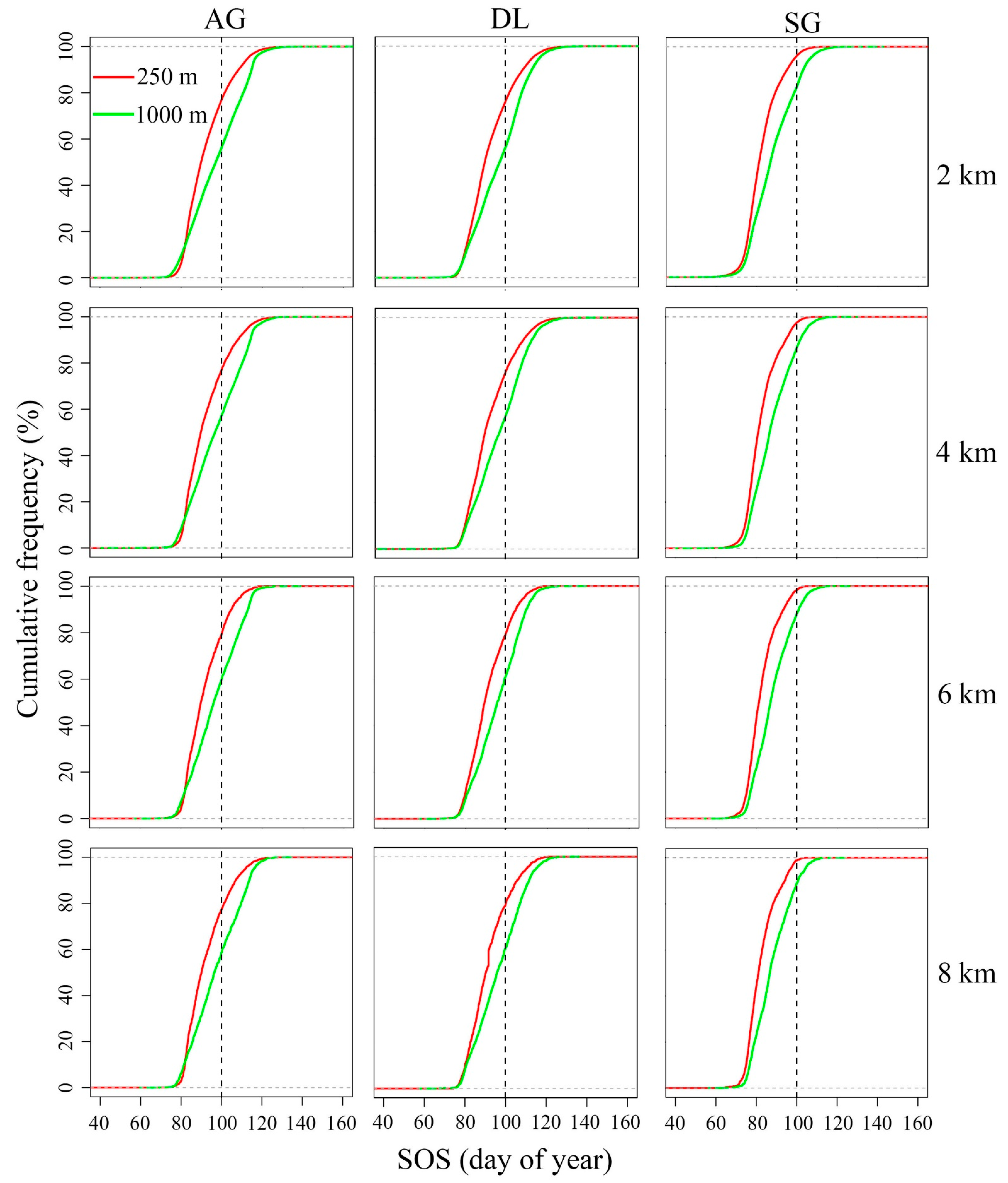
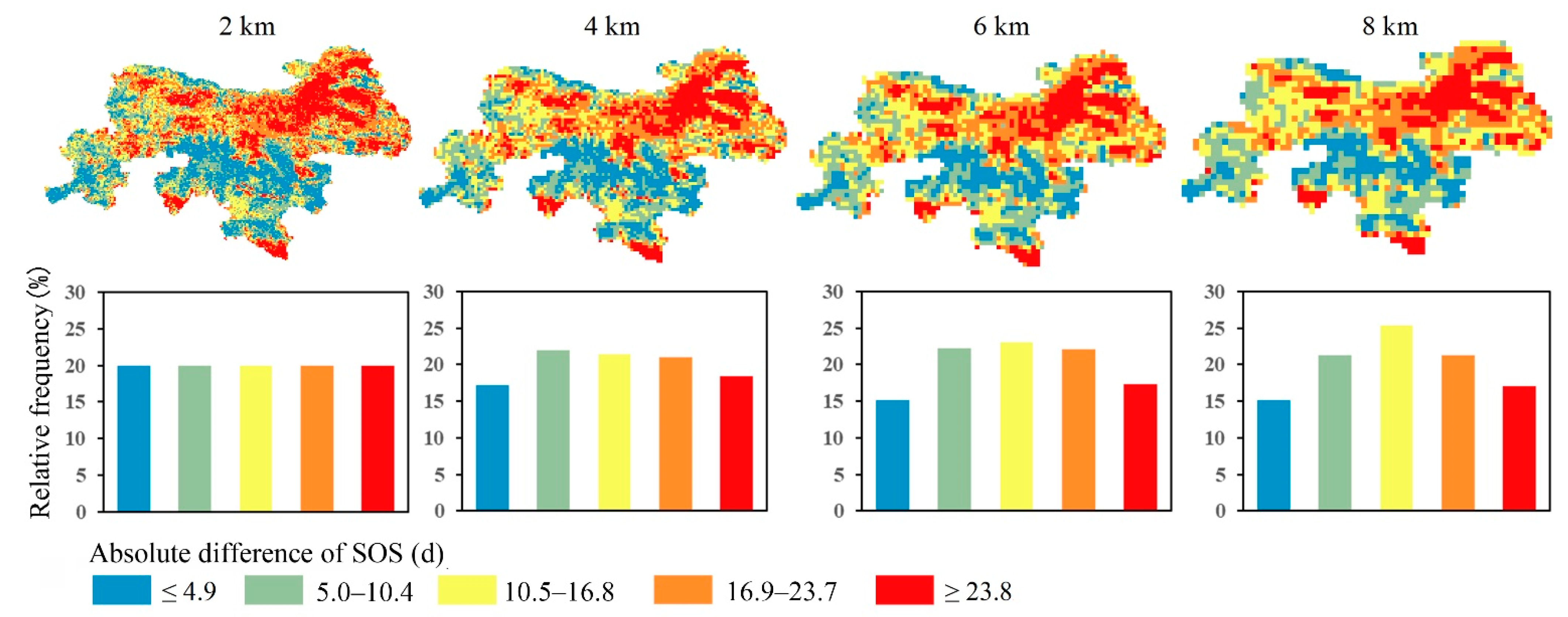
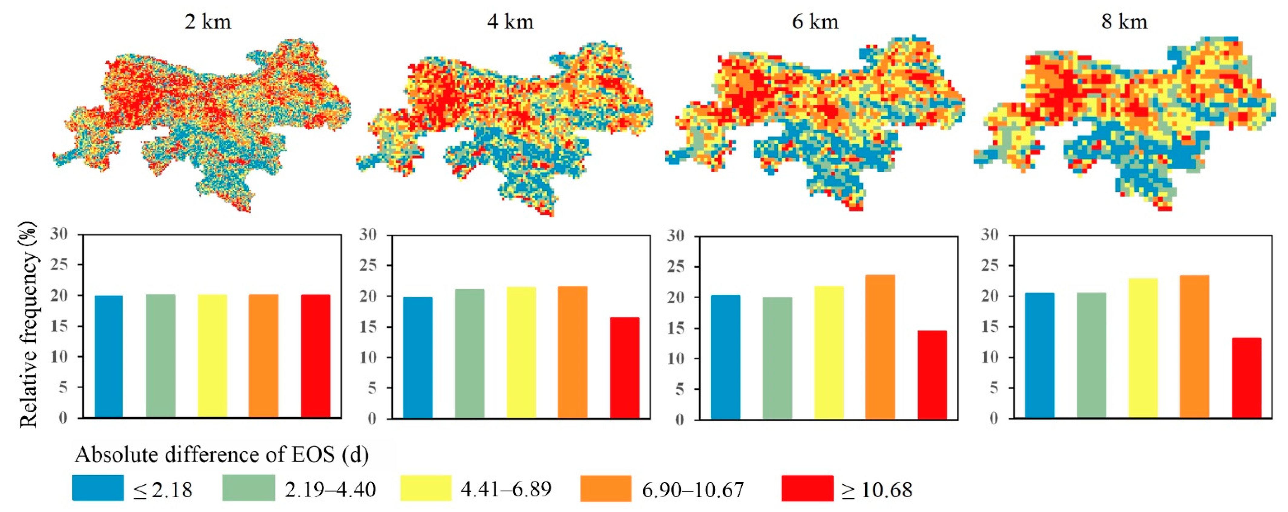
3.2.1. Quantitative Comparisons of the Up-Scaled SOSs

The simple linear regression R2 and the RMSE between each pair of the up-scaled SOSs at each scale is presented in Figure 8. All linear regression equations passed the F-test at a significance level of 0.001. This figure shows that the up-scaled SOSs are greatly impacted by both NDVI resolutions and the filtering methods. For SOSs derived from NDVI smoothed by the same filtering method, their up-scaled results derived from the 250 m SOSs are close to those derived from the 500 m SOSs, with higher R2 and lower RMSE. However, the results derived from the 1000 m SOSs are less close to the former two, with relatively low R2 or higher RMSE. For SOSs derived from NDVI processed by different filtering methods but with the same resolution, up-scaled SOSs from the AG- and DL-filtered data are closer to each other, but the up-scaled SOSs from the SG-filtered data are less close to the former two. This can be observed at all four scales. As the scale becomes larger, the R2 gets bigger and the RMSE becomes smaller in most cases, indicating the up-scaled SOSs are closer to each other at larger scales.
From the above analysis, up-scaled SOSs for the 500 m SOSs are extremely similar to those from 250 m. Hence, to illustrate upscaling effects, only the 250 m and 1000 m SOSs are shown here. The up-scaled SOS datasets from 250 m and 1000 m spatial resolution are shown in Figure 9 and Appendix A, Figure A1 and Figure A2. Consistent differences are seen from these figures. For example, at the ridge, the up-scaled 1000 m resolution SOS was significantly later than the 250 m resolution SOS (Appendix A, Figure A1 and Figure A2). The opposite behavior was observed for the slopes. Noticeable differences can also be seen in the CDF shapes at all four scales (Figure 9). In particular, the values of the up-scaled SOS from the 1000 m SOS are consistently higher than the corresponding SOS from the 250 m SOS, indicating a delayed green-up. Amongst the three filters, the SOS obtained from the AG-filtered NDVI was the most delayed and the SG-filtered SOS the most advanced.
The absolute differences between the up-scaled 250 m and 1000 m SOS based on the AG-filtered NDVI are shown in Figure 10. When the spatial scale was 2 km, the absolute difference in SOS in about 60% of the study area was <6.6 days, while 20% had differences >11.7 days. The difference was large in the northeastern regions, while it was small in the southern and western regions. As the spatial scale increased from 2 to 8 km, the spatial difference gradually decreased. At 8 km, less than 9% had differences >11.7 days, compared to 20% at 2 km.
The vegetation phenology differences were more prominent after datasets were up-scaled using different filtering methods than when the same filtering method was used (Figure 11). It shows that, as the spatial scale increased, the difference between the two datasets (i.e., 250 m SOS obtained through SG-filtering and the 1000 m SOS obtained through AG-filtering) was “intermediate”, which was more obvious than the trend demonstrated in Figure 9. Specifically, the areas under <4.9 d and >23.8 d showed a decreasing trend, and those between 5.0 and 23.7 d showed an increasing trend. This indicates that although different filtering methods can enlarge this difference, the increase in the scale can at the same time reduce this difference. This can also be proved by Figure 8.

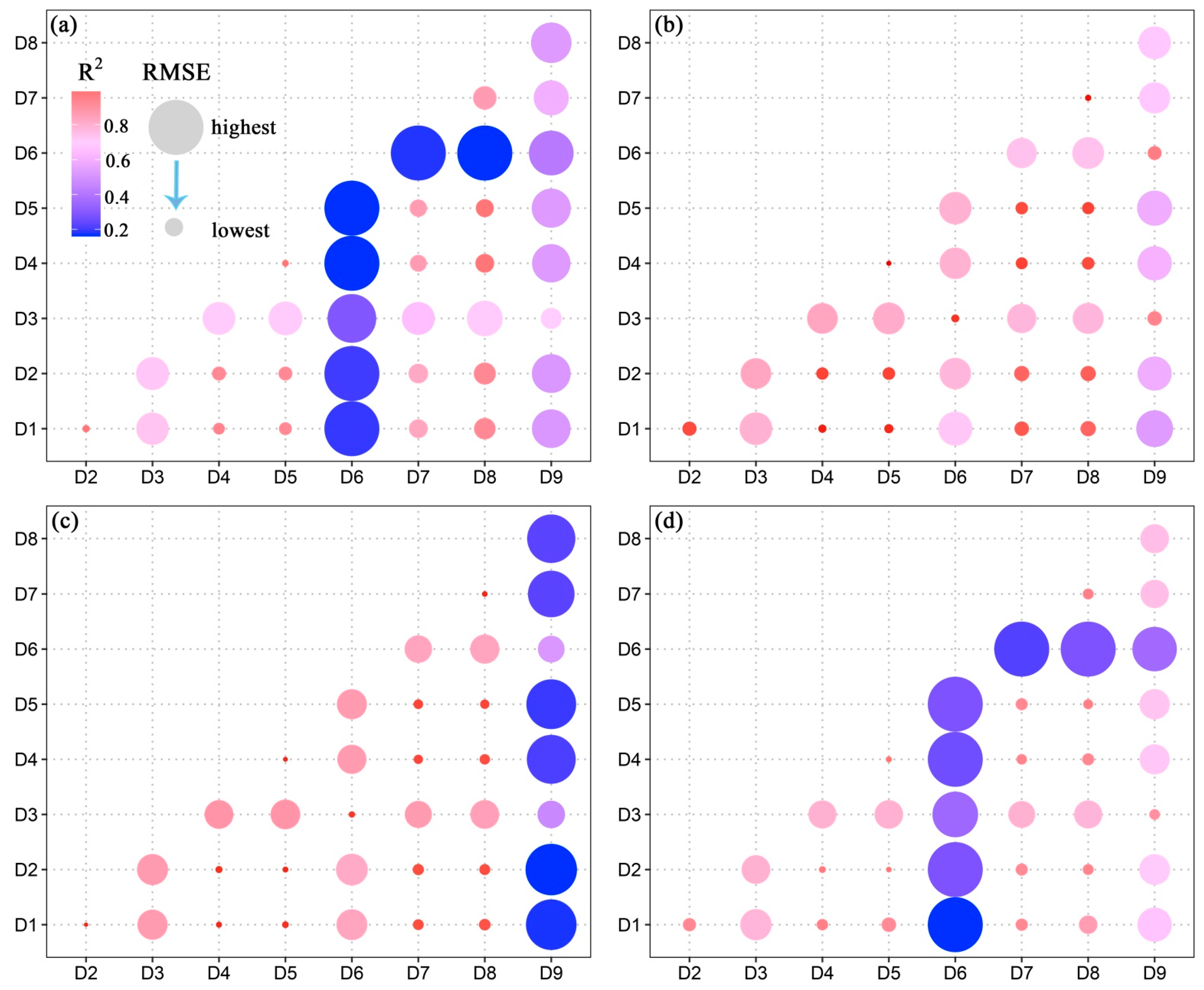
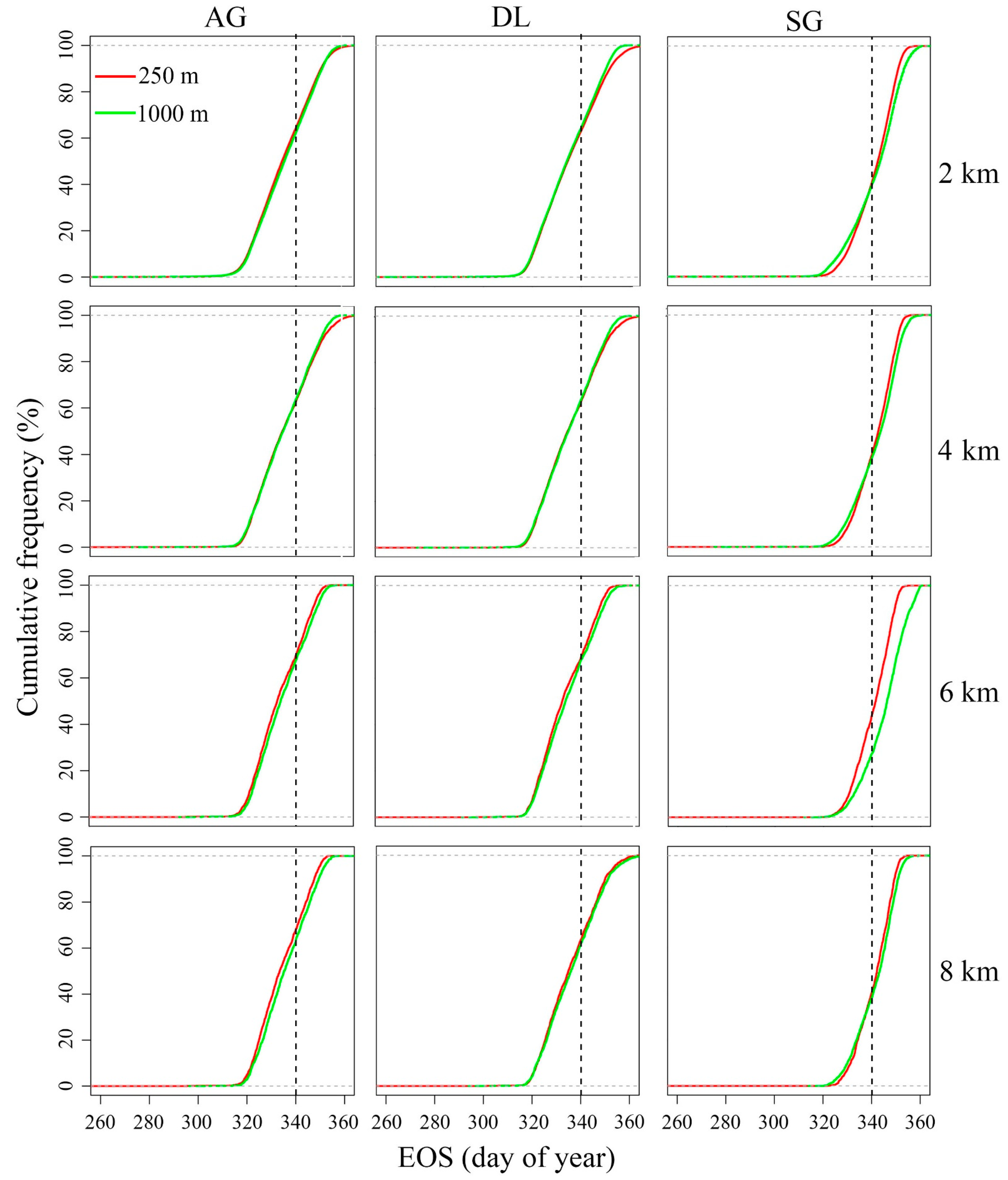
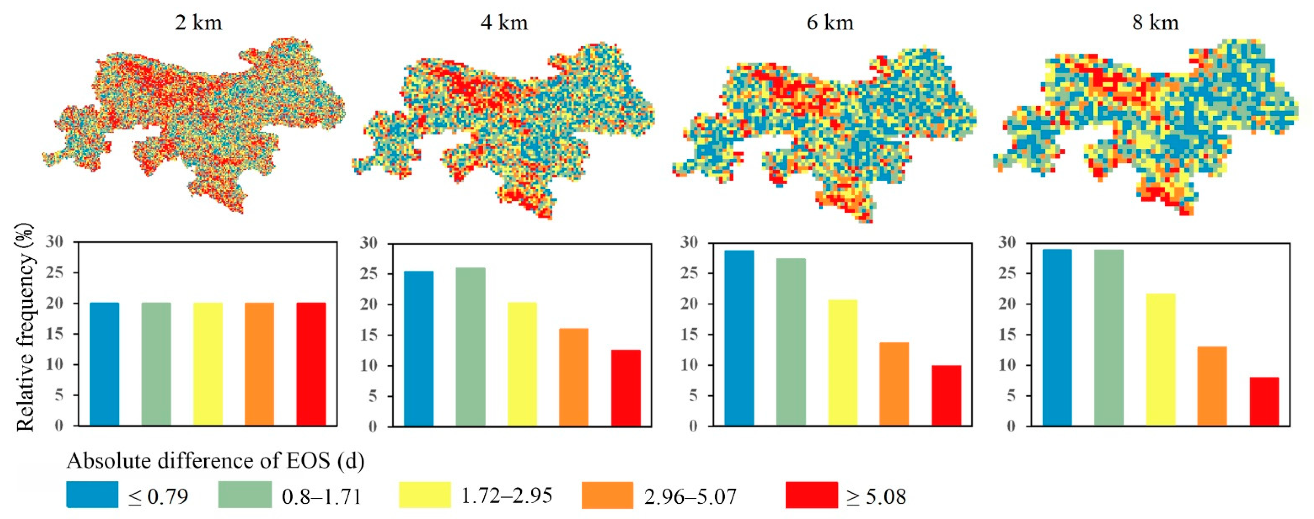
3.2.2. Quantitative Comparisons of the Up-Scaled EOSs

Similarly, the simple linear regression R2 and the RMSE between each pair of the up-scaled EOSs at each scale are drawn in Figure 12. All linear regression equations pass the F-test at a significance level of 0.001. Unlike the up-scaled SOSs, the up-scaled EOSs are mostly impacted by NDVI filtering methods. The up-scaled EOSs generated from EOSs derived from the SG-filtered NDVI are consistently different from those derived from the AG- and DL-filtered NDVI, with much lower R2 and relatively large RMSE, especially those from the 500 and 1000 m SG-filtered NDVI. Distinctly, the up-scaled EOSs at 4 km are all closer to each other than at other scales. This indicates that when the scale becomes larger, the up-scaled EOSs become similar then become slightly different.
As the same, to illustrate upscaling effects, only the 250 m and 1000 m EOS datasets are compared here. Figure 13 and Appendix A, Figure A3 and Figure A4 show the upscaling results of 250 m and 1000 m resolution EOS data (excluding outliers). The up-scaled EOS obtained by the three filtering methods was compared at the same scale. The up-scaled EOS retrieved by the AG filter was the earliest, while that retrieved by the DL filter ranged between AG- and SG-derived EOS. The EOS obtained by SG-filtering was approximately 8 d later than the AG-derived EOS. Unlike SOS, the CDFs show data distributions of the up-scaled EOS from the 250 m and 1000 m EOS that are very close to each other at all scales. Moreover, irrespective of the resolution and filtering method used to retrieve the EOS, the spatial difference of EOS gradually decreased from 2 km to 8 km with reductions in the spatial resolution.
Similar to the SOS results, we calculated the absolute difference of the 250 m and 1000 m EOS retrieved by AG-filtering (Figure 14). When the spatial scale was 2 km, the absolute difference was within 5 d in 80% of the study area. The absolute differences were largest in the northern ridge area, and smallest in the southern and western regions. As the scale increased, the spatial difference decreased gradually, and when the scale was 8 km, 80% of the study area showed an absolute difference of less than three days.
The absolute differences between the 250 m SOS retrieved by SG-filtering and the 1000 m EOS obtained by AG-filtering are shown in Figure 15. Similar to SOS, the difference between the EOS upscaling results with different resolutions was not evenly distributed spatially, and different filtering processing methods enlarged this difference, while an increasing scale reduced this difference. Our results indicate when smoothing NDVI time series in mountainous forest ecosystems, the filtering methods should be carefully inspected and selected.

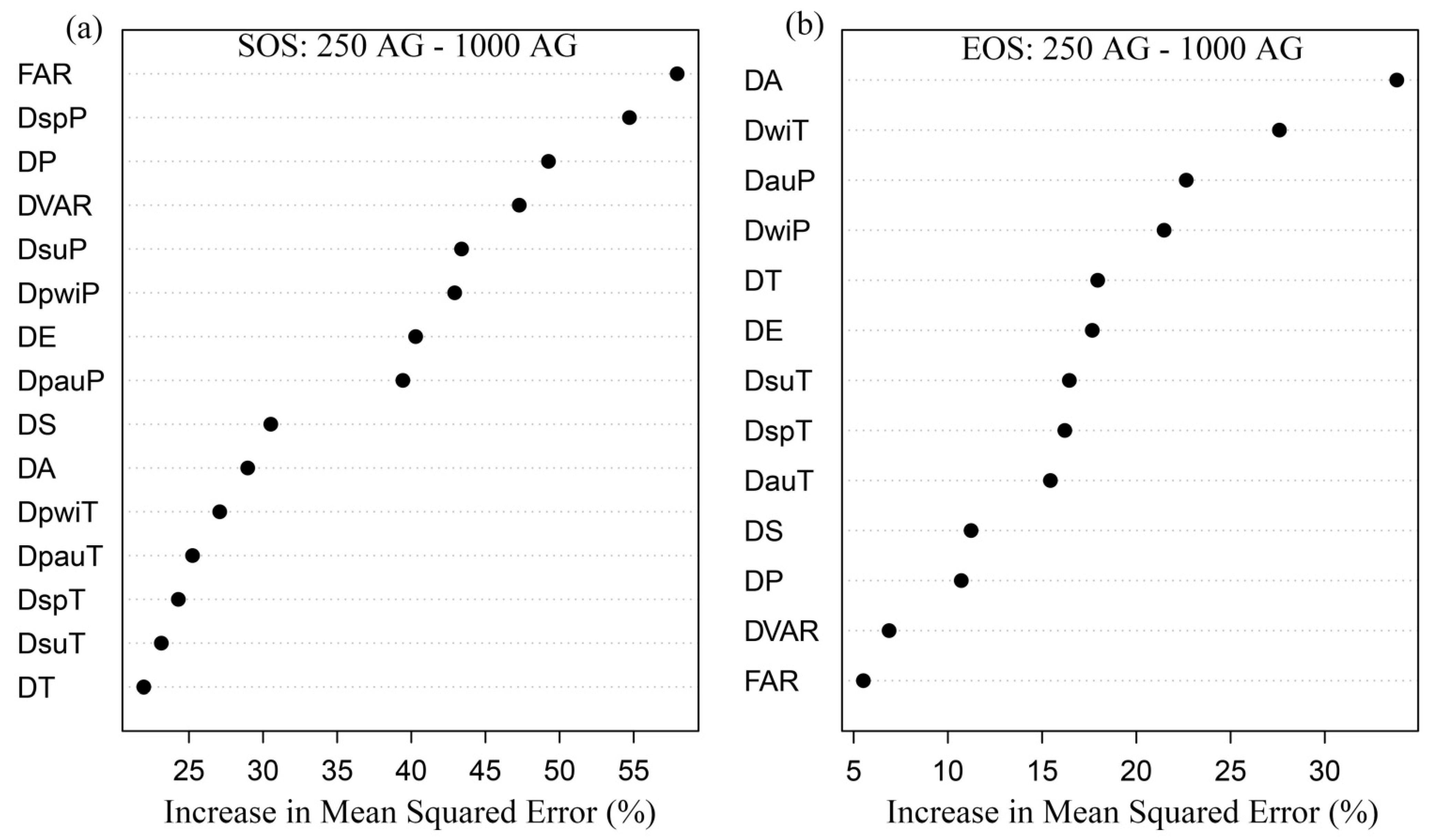
3.3. Major Factors Influencing LSP Spatial Scale Effect

We input all data from the four scales into the RF model, and the relative importance of the considered factors is shown in Figure 16. There are big differences between the major factors affecting the spatial scale effects of SOS and EOS. As for the spatial scale effect of SOS, the most important factors are forest cover, spring precipitation, and annual precipitation. This reveals that the differences observed in SOS across scales in Qinling Mountains are mainly caused by forest cover, uneven distribution of spring precipitation, and annual precipitation. The spatial variations in summer precipitation and previous winter precipitation also cause the observed SOS difference across different scales. Temperature factors have weak impact on SOS observation at different scales. On the contrary, spatial variations in aspect, winter temperature, and autumn precipitation all strongly influence the observed EOS at different scales, indicating that topographic heterogeneity and unevenly distributed meteorological conditions can strongly influence the observation of EOS across scales. In addition, spatial variations in winter precipitation have big impact on EOS observation across scales. Different from SOS, forest cover has very weak impact on the detected EOSs across scales in the Qinling Mountains.

4. Discussion

Long-term spatiotemporal changes in regional and global land surface phenology and its responses to climatic and environmental change have been extensively studied in the current research. However, the spatial scale effects in land surface phenology are seldom studied, especially in mountainous areas. We compared the upscaling differences in vegetation phenology based on various datasets in the Qinling Mountains. The up-scaled SOS was greatly impacted by both NDVI resolution and the filtering method, while the up-scaled EOS was mostly impacted by the filtering method. Our findings are consistent with existing research. For example, by using the same MODIS NDVI products as used in this study, Li et al. [76] compared the correlations between ground observations and the SOS retrieved from the three NDVI data in the mountains of northwest Mongolia, and found the SOS derived from the high resolution MOD13Q1 NDVI had the strongest correlations with ground truths. Similarly, Mountford et al. [77] investigated the SOS/EOS across the entire United Kingdom and found that remotely sensed phenological parameters are sensitive to spatial resolution and composite period.
Different filtering processing methods enlarged the difference between different up-scaled vegetation phenology in the Qinling Mountains, while up-scaling reduced this difference. Different filtering methods have different assumptions and utilize different mathematic methods to smooth NDVI time series, which alters the shape of NDVI time series and eventually impacts the retrieved SOS/EOS. Our findings indicate when smoothing NDVI time series in mountainous forest ecosystem, the filtering methods should be carefully inspected and selected. The spatial averaging method was used for up-scaling SOS and EOS. Since the spatial averaging tends to eliminate the differences between pixels in grids, making the results move toward the regional mean. Thus, it blurs the differences between the up-scaled SOSs/EOSs. Although this method is easy to use, some studies have reported that the phenology obtained by this method differs from that retrieved from coarse resolution data [5]. In contrast, the percentile method can reduce the inconsistency in phenological data retrieval at different scales by selecting the SOS/EOS corresponding to different percentiles [5,34]. However, the percentile method is highly empirical. Determining the appropriate percentile, which varies regionally, requires appropriate validation data [34]. Thus, the most suitable percentiles for different regions are difficult to determine.
Elevation has been identified as a significant contributor of the phenology variability [76,78]. In mountain ecosystems, topography greatly influences the microclimate, community composition, and available soil moisture [79]. Prominent spatial scale effects of vegetation phenology are observed in the Qinling Mountains in our study. While the difference observed in SOS across scales in Qinling Mountains are mainly caused by forest cover, uneven distribution of spring precipitation, and annual precipitation, the aspect heterogeneity and unevenly distributed winter temperature and autumn precipitation strongly influence the observation of EOS across scales. The possible reason is that an increase in spring precipitation in mountain areas may make soil moisture reach its optimal state for vegetation to grow earlier [80]. As Qinling Mountains are dominated by forest, a higher forest cover means less shrub and grass exist, thus the start of season will show less heterogeneity. It has been well recognized in existing studies that warmer autumn leads to a later EOS [81,82]. The temperature in mountain areas is usually lower than the plains at the same latitude. As sunny slopes receive more sunlight and are low in water content, it favors the growth of sun loving plants. Shady slopes, on the contrary, receive less sunlight and are high in humidity; thus, they are suitable for the growth of shade loving plants. In this way, the aspect affects the microclimate, which ultimately affects the vegetation phenology. A higher temperature in winter in Qinling Mountains will extend the photosynthetic activities of vegetation [83]. Increased precipitation in autumn will improve the soil moisture and delay vegetation senescence. Our findings not only provide a useful supplement to the existing literature on the analysis of factors affecting the long-term variations of phenology in the same area [45,68,70,71], but also strongly confirm the discoveries in previous studies in other forest mountain regions, such as Peng et al. [84]. Therefore, the spatial scale effects of vegetation phenology in mountain areas should not be neglected in future related studies.
A series of ecological projects has been implemented in the past two decades in Qinling Mountains to prevent vegetation degradation and help vegetation recovery, such as the Grain for Green program, the Natural Forest Protection project, the Establishment of Nature Reserves, and the Project of Biodiversity Protection. Vegetation cover in this region increased notably, but problems still exit. As there are many on-going ecological restoration projects planned in Qinling Mountains, our findings about the factors influencing vegetation phenology could serve as an essential reference for vegetation restoration practice.

5. Conclusions

Quantifying the differences and identifying the influencing factors of vegetation phenology using remote sensing data with different spatial resolutions is significant for understanding the spatial scale effects of land surface phenology. This study qualitatively and quantitatively analyzed the vegetation phenology discrepancy across different scales in the Qinling Mountains, and the major factors influencing LSP spatial scale effect were also detected. The derived basic SOS/EOS datasets by the same filtering method from the 250 m and 500 m NDVI datasets are consistent in spatial distributions, while the results from the 1000 m NDVI dataset differ. For both basic and the up-scaled datasets, the LSP derived from the SG-filtered NDVI showed advance in SOS, but delay in EOS, compared to those derived from the AG- and DL-filtered NDVI. The up-scaled SOS was greatly impacted by both NDVI resolution and the filtering method. EOS, on the other hand, was only impacted by the filtering method. Moreover, up-scaled SOS had usually larger differences compared to up-scaled EOS. While different filtering methods sometimes amplified the absolute differences between different SOS/EOS across scales, the upscaling reduced the differences. Influence factor analysis showed that the spatial variations observed in SOS in Qinling Mountains are mainly caused by forest cover, uneven distribution of spring precipitation, and annual precipitation, while spatial variations in aspect, winter temperature, and autumn precipitation all strongly influence the observed EOS across scales in the study area. Our findings have significant implications for understanding the effects of observational scale on vegetation phenology and ecology in the Qinling Mountains.

Author Contributions

Data curation, M.M., M.L., X.L. and Z.D.; Formal analysis, M.M., J.L., W.Z. and C.A.; Funding acquisition, J.L.; Methodology, M.M., J.L., W.Z. and C.A.; Supervision, J.L.; Writing—original draft, M.M. and J.L.; Writing—review and editing, J.L., C.A. and W.Z. All authors have read and agreed to the published version of the manuscript.

Funding

This research was funded by National Natural Science Foundation of China (No. 41401494) and the Natural Science Foundation of Shaanxi Province (2021JQ-563).

Data Availability Statement

Not applicable.

Conflicts of Interest

The authors declare no conflict of interest.

Appendix A

Figure A1. Up-scaled SOSs from 250 m SOSs. (SG, Savitzky-Golay; AG, asymmetric Gaussian; DL, double logistic.)
Remotesensing 14 05749 g0a1
Figure A2. Up-scaled SOSs from 1000 m SOSs. (SG, Savitzky-Golay; AG, asymmetric Gaussian; DL, double logistic.)
Remotesensing 14 05749 g0a2
Figure A3. Up-scaled EOSs from 250 m EOSs. (SG, Savitzky-Golay; AG, asymmetric Gaussian; DL, double logistic.)
Remotesensing 14 05749 g0a3
Figure A4. Up-scaled EOSs from 1000 m EOSs. (SG, Savitzky-Golay; AG, asymmetric Gaussian; DL, double logistic.)
Remotesensing 14 05749 g0a4

References

  1. Zeng, L.; Wardlow, B.D.; Xiang, D.; Hu, S.; Li, D. A review of vegetation phenological metrics extraction using time-series, multispectral satellite data. Remote Sens. Environ. 2020, 237, 111511. [Google Scholar] [CrossRef]
  2. Yang, Y.; Ren, W.; Tao, B.; Ji, L.; Liang, L.; Ruane, A.C.; Fisher, J.B.; Liu, J.; Sama, M.; Li, Z.; et al. Characterizing spatiotemporal patterns of crop phenology across North America during 2000–2016 using satellite imagery and agricultural survey data. ISPRS J. Photogramm. Remote Sens. 2020, 170, 156–173. [Google Scholar] [CrossRef]
  3. Peng, D.; Zhang, X.; Zhang, B.; Liu, L.; Liu, X.; Huete, A.R.; Huang, W.; Wang, S.; Luo, S.; Zhang, X.; et al. Scaling effects on spring phenology detections from MODIS data at multiple spatial resolutions over the contiguous United States. ISPRS J. Photogramm. Remote Sens. 2017, 132, 185–198. [Google Scholar] [CrossRef]
  4. Wang, J.; Yang, D.; Detto, M.; Nelson, B.W.; Chen, M.; Guan, K.; Wu, S.; Yan, Z.; Wu, J. Multi-scale integration of satellite remote sensing improves characterization of dry-season green-up in an Amazon tropical evergreen forest. Remote Sens. Environ. 2020, 246, 111865. [Google Scholar] [CrossRef]
  5. Peng, D.; Wu, C.; Zhang, X.; Yu, L.; Huete, A.R.; Wang, F.; Luo, S.; Liu, X.; Zhang, H. Scaling up spring phenology derived from remote sensing images. Agric. For. Meteorol. 2018, 256–257, 207–219. [Google Scholar] [CrossRef]
  6. Li, X.; Du, H.; Zhou, G.; Mao, F.; Zhang, M.; Han, N.; Fan, W.; Liu, H.; Huang, Z.; He, S.; et al. Phenology estimation of subtropical bamboo forests based on assimilated MODIS LAI time series data. ISPRS J. Photogramm. Remote Sens. 2021, 173, 262–277. [Google Scholar] [CrossRef]
  7. Bolton, D.K.; Gray, J.M.; Melaas, E.K.; Moon, M.; Eklundh, L.; Friedl, M.A. Continental-scale land surface phenology from harmonized Landsat 8 and Sentinel-2 imagery. Remote Sens. Environ. 2020, 240, 111685. [Google Scholar] [CrossRef]
  8. He, L.; Jin, N.; Yu, Q. Impacts of climate change and crop management practices on soybean phenology changes in China. Sci. Total Environ. 2020, 707, 135638. [Google Scholar] [CrossRef]
  9. Klosterman, S.; Melaas, E.; Wang, J.A.; Martinez, A.; Frederick, S.; O’Keefe, J.; Orwig, D.A.; Wang, Z.; Sun, Q.; Schaaf, C.; et al. Fine-scale perspectives on landscape phenology from unmanned aerial vehicle (UAV) photography. Agric. For. Meteorol. 2018, 248, 397–407. [Google Scholar] [CrossRef]
  10. Li, D.; Wang, Z. Spatiotemporal Variation of Vegetation Phenology and Its Response to Climate in Qinling Mountains Based on MCD12Q2. Ecol. Environ. Sci. 2020, 29, 11–22. [Google Scholar] [CrossRef]
  11. Zhu, W.; Chen, G.; Jiang, N.; Liu, J.; Mou, M. Estimating Carbon Flux Phenology with Satellite-Derived Land Surface Phenology and Climate Drivers for Different Biomes: A Synthesis of AmeriFlux Observations. PLoS ONE 2013, 8, e84990. [Google Scholar] [CrossRef] [PubMed] [Green Version]
  12. Shahzaman, M.; Zhu, W.; Ullah, I.; Mustafa, F.; Bilal, M.; Ishfaq, S.; Nisar, S.; Arshad, M.; Iqbal, R.; Aslam, R.W. Comparison of Multi-Year Reanalysis, Models, and Satellite Remote Sensing Products for Agricultural Drought Monitoring over South Asian Countries. Remote Sens. 2021, 13, 3294. [Google Scholar] [CrossRef]
  13. Bouras, E.; Jarlan, L.; Er-Raki, S.; Balaghi, R.; Amazirh, A.; Richard, B.; Khabba, S. Cereal Yield Forecasting with Satellite Drought-Based Indices, Weather Data and Regional Climate Indices Using Machine Learning in Morocco. Remote Sens. 2021, 13, 3101. [Google Scholar] [CrossRef]
  14. Wang, H.; Magagi, R.; Goïta, K.; Trudel, M.; McNairn, H.; Powers, J. Crop phenology retrieval via polarimetric SAR decomposition and Random Forest algorithm. Remote Sens. Environ. 2019, 231, 111234. [Google Scholar] [CrossRef]
  15. Meroni, M.; Atzberger, C.; Vancutsem, C.; Gobron, N.; Baret, F.; Lacaze, R.; Eerens, H.; Leo, O. Evaluation of Agreement Between Space Remote Sensing SPOT-VEGETATION fAPAR Time Series. IEEE Trans. Geosci. Remote Sens. 2013, 51, 1951–1962. [Google Scholar] [CrossRef]
  16. Atzberger, C.; Eilers, P.H. A time series for monitoring vegetation activity and phenology at 10-daily time steps covering large parts of South America. Int. J. Digit. Earth 2011, 4, 365–386. [Google Scholar] [CrossRef]
  17. Fang, F.; McNeil, B.E.; Warner, T.A.; Maxwell, A.E.; Dahle, G.A.; Eutsler, E.; Li, J. Discriminating tree species at different taxonomic levels using multi-temporal WorldView-3 imagery in Washington D.C., USA. Remote Sens. Environ. 2020, 246, 111811. [Google Scholar] [CrossRef]
  18. Xu, Z.; Liu, Q.; Du, W.; Zhou, G.; Qin, L.; Sun, Z. Modelling leaf phenology of some trees with accumulated temperature in a temperate forest in northeast China. For. Ecol. Manag. 2021, 489, 119085. [Google Scholar] [CrossRef]
  19. Wu, S.; Wang, J.; Yan, Z.; Song, G.; Chen, Y.; Ma, Q.; Deng, M.; Wu, Y.; Zhao, Y.; Guo, Z.; et al. Monitoring tree-crown scale autumn leaf phenology in a temperate forest with an integration of PlanetScope and drone remote sensing observations. ISPRS J. Photogramm. Remote Sens. 2021, 171, 36–48. [Google Scholar] [CrossRef]
  20. Shen, M.; Jiang, N.; Peng, D.; Rao, Y.; Huang, Y.; Fu, Y.H.; Yang, W.; Zhu, X.; Cao, R.; Chen, X.; et al. Can changes in autumn phenology facilitate earlier green-up date of northern vegetation? Agric. For. Meteorol. 2020, 291, 108077. [Google Scholar] [CrossRef]
  21. Xie, Y.; Wilson, A.M. Change point estimation of deciduous forest land surface phenology. Remote Sens. Environ. 2020, 240, 111698. [Google Scholar] [CrossRef]
  22. Li, P.; Liu, Z.; Zhou, X.; Xie, B.; Li, Z.; Luo, Y.; Zhu, Q.; Peng, C. Combined control of multiple extreme climate stressors on autumn vegetation phenology on the Tibetan Plateau under past and future climate change. Agric. For. Meteorol. 2021, 308–309, 108571. [Google Scholar] [CrossRef]
  23. Chen, X.; Hu, B.; Yu, R. Spatial and temporal variation of phenological growing season and climate change impacts in temperate eastern China. Glob. Chang. Biol. 2005, 11, 1118–1130. [Google Scholar] [CrossRef]
  24. Zhang, X. Land surface phenology: Climate data record and real-time monitoring. Compr. Remote Sens. 2018, 3, 35–52. [Google Scholar] [CrossRef]
  25. Xia, C.; Li, J.; Huo, Q. Review of advances in vegetation phenology monitoring by remote sensing. J. Remote Sens. 2013, 17, 1–16. [Google Scholar] [CrossRef]
  26. Morisette, J.T.; Baret, F.; Privette, J.L.; Myneni, R.B.; Nickeson, J.E.; Garrigues, S.; Shabanov, N.V.; Weiss, M.; Fernandes, R.A.; Leblanc, S.G.; et al. Validation of global moderate-resolution LAI products: A framework proposed within the CEOS land product validation subgroup. IEEE Trans. Geosci. Remote Sens. 2006, 44, 1804–1817. [Google Scholar] [CrossRef] [Green Version]
  27. Chen, J.; Jönsson, P.; Tamura, M.; Gu, Z.; Matsushita, B.; Eklundh, L. A simple method for reconstructing a high-quality NDVI time-series data set based on the Savitzky–Golay filter. Remote Sens. Environ. 2004, 91, 332–344. [Google Scholar] [CrossRef]
  28. Bai, Y. Analysis of vegetation dynamics in the Qinling-Daba Mountains region from MODIS time series data. Ecol. Indic. 2021, 129, 108029. [Google Scholar] [CrossRef]
  29. Gao, X.; Gray, J.M.; Reich, B.J. Long-term, medium spatial resolution annual land surface phenology with a Bayesian hierarchical model. Remote Sens. Environ. 2021, 261, 112484. [Google Scholar] [CrossRef]
  30. Yang, H.; Pan, B.; Li, N.; Wang, W.; Zhang, J.; Zhang, X. A systematic method for spatio-temporal phenology estimation of paddy rice using time series Sentinel-1 images. Remote Sens. Environ. 2021, 259, 112394. [Google Scholar] [CrossRef]
  31. Park, D.S.; Newman, E.A.; Breckheimer, I.K. Scale gaps in landscape phenology: Challenges and opportunities. Trends Ecol. Evol. 2021, 36, 709–721. [Google Scholar] [CrossRef] [PubMed]
  32. Atkinson, P.M.; Jeganathan, C.; Dash, J.; Atzberger, C. Inter-comparison of four models for smoothing satellite sensor time-series data to estimate vegetation phenology. Remote Sens. Environ. 2012, 123, 400–417. [Google Scholar] [CrossRef]
  33. Atzberger, C.; Eilers, P.H.C. Evaluating the effectiveness of smoothing algorithms in the absence of ground reference measurements. Int. J. Remote Sens. 2011, 32, 3689–3709. [Google Scholar] [CrossRef]
  34. Zhang, X.; Wang, J.; Gao, F.; Liu, Y.; Schaaf, C.; Friedl, M.; Yu, Y.; Jayavelu, S.; Gray, J.; Liu, L.; et al. Exploration of scaling effects on coarse resolution land surface phenology. Remote Sens. Environ. 2017, 190, 318–330. [Google Scholar] [CrossRef] [Green Version]
  35. Peng, D.; Wang, Y.; Xian, G.; Huete, A.R.; Huang, W.; Shen, M.; Wang, F.; Yu, L.; Liu, L.; Xie, Q.; et al. Investigation of land surface phenology detections in shrublands using multiple scale satellite data. Remote Sens. Environ. 2021, 252, 112133. [Google Scholar] [CrossRef]
  36. Qi, G.; Song, J.; Li, Q.; Bai, H.; Sun, H.; Zhang, S.; Cheng, D. Response of vegetation to multi-timescales drought in the Qinling Mountains of China. Ecol. Indic. 2022, 135, 108539. [Google Scholar] [CrossRef]
  37. Fisher, J.I.; Mustard, J.F. Cross-scalar satellite phenology from ground, Landsat, and MODIS data. Remote Sens. Environ. 2007, 109, 261–273. [Google Scholar] [CrossRef]
  38. Delbart, N.; Beaubien, E.; Kergoat, L.; Le Toan, T. Comparing land surface phenology with leafing and flowering observations from the PlantWatch citizen network. Remote Sens. Environ. 2015, 160, 273–280. [Google Scholar] [CrossRef]
  39. Zhang, H.; Gao, Y.; Hua, Y.; Zhang, Y.; Liu, K. Assessing and mapping recreationists’ perceived social values for ecosystem services in the Qinling Mountains, China. Ecosyst. Serv. 2019, 39, 101006. [Google Scholar] [CrossRef]
  40. Wang, B.; Xu, G.; Li, P.; Li, Z.; Zhang, Y.; Cheng, Y.; Jia, L.; Zhang, J. Vegetation dynamics and their relationships with climatic factors in the Qinling Mountains of China. Ecol. Indic. 2020, 108, 105719. [Google Scholar] [CrossRef]
  41. Jun, C.; Ban, Y.; Li, S. Open access to Earth land-cover map. Nature 2014, 514, 434. [Google Scholar] [CrossRef] [PubMed] [Green Version]
  42. Zhang, Y.; Liu, X.; Jiao, W.; Zhao, L.; Zeng, X.; Xing, X.; Zhang, L.; Hong, Y.; Lu, Q. A new multi-variable integrated framework for identifying flash drought in the Loess Plateau and Qinling Mountains regions of China. Agric. Water Manag. 2022, 265, 107544. [Google Scholar] [CrossRef]
  43. Sisheber, B.; Marshall, M.; Mengistu, D.; Nelson, A. Tracking crop phenology in a highly dynamic landscape with knowledge-based Landsat–MODIS data fusion. Int. J. Appl. Earth Obs. Geoinf. 2022, 106, 102670. [Google Scholar] [CrossRef]
  44. Ma, X.; Bai, H.; He, Y.; Qin, J. The Vegetation Remote Sensing Phenology of Qinling Mountains Based on NDVI and It‘s Response to Temperature: Taking Within the Territory of Shaanxi as An Example. Sci. Geogr. Sin. 2015, 35, 1616–1621. [Google Scholar] [CrossRef]
  45. Xia, H.; Qin, Y.; Feng, G.; Meng, Q.; Cui, Y.; Song, H.; Ouyang, Y.; Liu, G. Forest Phenology Dynamics to Climate Change and Topography in a Geographic and Climate Transition Zone: The Qinling Mountains in Central China. Forests 2019, 10, 1007. [Google Scholar] [CrossRef] [Green Version]
  46. Zhao, F.; Zhang, B.; Zhu, L.; Yao, Y.; Cui, Y.; Liu, J. Spectra structures of altitudinal belts and their aignificance for determining the boundary between warm temperate and subtropical zones in the Qinling-Daba Mountains. J. Remote Sens. 2019, 74, 889–901. [Google Scholar] [CrossRef]
  47. Touhami, I.; Moutahir, H.; Assoul, D.; Bergaoui, K.; Aouinti, H.; Bellot, J.; Andreu, J.M. Multi-year monitoring land surface phenology in relation to climatic variables using MODIS-NDVI time-series in Mediterranean forest, Northeast Tunisia. Acta Oecologica 2022, 114, 103804. [Google Scholar] [CrossRef]
  48. Yang, C.; Deng, K.; Peng, D.; Jiang, L.; Zhao, M.; Liu, J.; Qiu, X. Spatiotemporal Characteristics and Heterogeneity of Vegetation Phenology in the Yangtze River Delta. Remote Sens. 2022, 14, 2984. [Google Scholar] [CrossRef]
  49. Peng, S.; Ding, Y.; Liu, W.; Li, Z. 1 km monthly temperature and precipitation dataset for China from 1901 to 2017. Earth Syst. Sci. Data 2019, 11, 1931–1946. [Google Scholar] [CrossRef] [Green Version]
  50. Jie, C.; Shengyue, D.; Jiancheng, S. 1km seamless land surface temperature dataset of China (2002–2020). Natl. Tibet. Plateau Data Cent. 2021. Available online: https://data.tpdc.ac.cn/en/data/7e5333df-0208-4c4e-ae7e-16dcd29e4aa7/ (accessed on 19 July 2022). [CrossRef]
  51. Zhang, Q.; Cheng, J. An Empirical Algorithm for Retrieving Land Surface Temperature From AMSR-E Data Considering the Comprehensive Effects of Environmental Variables. Earth Space Sci. 2020, 7, e2019EA001006. [Google Scholar] [CrossRef] [Green Version]
  52. Xu, S.; Cheng, J. A new land surface temperature fusion strategy based on cumulative distribution function matching and multiresolution Kalman filtering. Remote Sens. Environ. 2021, 254, 112256. [Google Scholar] [CrossRef]
  53. Zhang, Q.; Wang, N.; Cheng, J.; Xu, S. A Stepwise Downscaling Method for Generating High-Resolution Land Surface Temperature From AMSR-E Data. IEEE J. Sel. Top. Appl. Earth Obs. Remote Sens. 2020, 13, 5669–5681. [Google Scholar] [CrossRef]
  54. Shouzhang, P. 1-km monthly precipitation dataset for China (1901–2021). Natl. Tibet. Plateau Data Cent. 2020. [Google Scholar] [CrossRef]
  55. Peng, S.; Ding, Y.; Wen, Z.; Chen, Y.; Cao, Y.; Ren, J. Spatiotemporal change and trend analysis of potential evapotranspiration over the Loess Plateau of China during 2011–2100. Agric. For. Meteorol. 2017, 233, 183–194. [Google Scholar] [CrossRef] [Green Version]
  56. Ding, Y.; Peng, S. Spatiotemporal Trends and Attribution of Drought across China from 1901–2100. Sustainability 2020, 12, 477. [Google Scholar] [CrossRef] [Green Version]
  57. National Aeronautics and Space Administration. Available online: https://search.asf.alaska.edu/#/ (accessed on 7 January 2021).
  58. Li, S.; Xu, L.; Jing, Y.; Yin, H.; Li, X.; Guan, X. High-quality vegetation index product generation: A review of NDVI time series reconstruction techniques. Int. J. Appl. Earth Obs. Geoinf. 2021, 105, 102640. [Google Scholar] [CrossRef]
  59. Zhou, J.; Jia, L.; Menenti, M.; Gorte, B. On the performance of remote sensing time series reconstruction methods—A spatial comparison. Remote Sens. Environ. 2016, 187, 367–384. [Google Scholar] [CrossRef]
  60. Jönsson, P.; Eklundh, L. TIMESAT—A program for analyzing time-series of satellite sensor data. Comput. Geosci. 2004, 30, 833–845. [Google Scholar] [CrossRef] [Green Version]
  61. Jonsson, P.; Eklundh, L. Seasonality extraction by function fitting to time-series of satellite sensor data. IEEE Trans. Geosci. Remote Sens. 2002, 40, 1824–1832. [Google Scholar] [CrossRef]
  62. Savitzky, A.; Golay, M.J.E. Smoothing and Differentiation of Data by Simplified Least Squares Procedures. Anal. Chem. 1964, 36, 1627–1639. [Google Scholar] [CrossRef]
  63. Yang, B.; Xu, H.; Jiang, L.; Huang, R.; Zhou, Z.; Wang, H.; Liu, W. A Multicomponent Temporal Coherence Model for 3-D Phase Unwrapping in Time-Series InSAR of Seasonal Deformation Areas. Remote Sens. 2022, 14, 1080. [Google Scholar] [CrossRef]
  64. Liu, L.; Cao, R.; Shen, M.; Chen, J.; Wang, J.; Zhang, X. How Does Scale Effect Influence Spring Vegetation Phenology Estimated from Satellite-Derived Vegetation Indexes? Remote Sens. 2019, 11, 2137. [Google Scholar] [CrossRef] [Green Version]
  65. Piao, S.; Liu, Q.; Chen, A.; Janssens, I.; Fu, Y.; Dai, J.; Liu, L.; Lian, X.; Shen, M.; Zhu, X. Plant phenology and global climate change: Current progresses and challenges. Glob. Chang. Biol. 2019, 25, 1922–1940. [Google Scholar] [CrossRef] [PubMed]
  66. Spiess, A.-N.; Neumeyer, N. An evaluation of R2 as an inadequate measure for nonlinear models in pharmacological and biochemical research: A Monte Carlo approach. BMC Pharmacol. 2010, 10, 6. [Google Scholar] [CrossRef] [Green Version]
  67. Shrestha, R.; Di, L.; Yu, E.G.; Kang, L.; Shao, Y.-Z.; Bai, Y.-Q. Regression model to estimate flood impact on corn yield using MODIS NDVI and USDA cropland data layer. J. Integr. Agric. 2017, 16, 398–407. [Google Scholar] [CrossRef] [Green Version]
  68. Yin, C.; Yang, Y.; Yang, F.; Chen, X.; Xin, Y.; Luo, P. Diagnose the dominant climate factors and periods of spring phenology in Qinling Mountains, China. Ecol. Indic. 2021, 131, 108211. [Google Scholar] [CrossRef]
  69. Wang, Z.; Xue, C.; Quan, W.; He, H. Spatiotemporal variations of forest phenology in the Qinling Mountains and its response to a critical temperature of 10 °C. J. Appl. Remote Sens. 2018, 12, 022202. [Google Scholar] [CrossRef] [Green Version]
  70. Guo, J.; Liu, X.; Ge, W.; Ni, X.; Ma, W.; Lu, Q.; Xing, X. Specific Drivers and Responses to Land Surface Phenology of Different Vegetation Types in the Qinling Mountains, Central China. Remote Sens. 2021, 13, 4538. [Google Scholar] [CrossRef]
  71. Deng, C.; Ma, X.; Xie, M.; Bai, H. Effect of Altitude and Topography on Vegetation Phenological Changes in the Niubeiliang Nature Reserve of Qinling Mountains, China. Forests 2022, 13, 1229. [Google Scholar] [CrossRef]
  72. Belgiu, M.; Drăguţ, L. Random forest in remote sensing: A review of applications and future directions. ISPRS J. Photogramm. Remote Sens. 2016, 114, 24–31. [Google Scholar] [CrossRef]
  73. Mohana, R.M.; Reddy, C.K.K.; Anisha, P.; Murthy, B.R. Random forest algorithms for the classification of tree-based ensemble. Mater. Today Proc. 2021. [Google Scholar] [CrossRef]
  74. Liu, M.; Liu, J.; Atzberger, C.; Jiang, Y.; Ma, M.; Wang, X. Zanthoxylum bungeanum Maxim mapping with multi-temporal Sentinel-2 images: The importance of different features and consistency of results. ISPRS J. Photogramm. Remote Sens. 2021, 174, 68–86. [Google Scholar] [CrossRef]
  75. Ma, M.; Liu, J.; Liu, M.; Zeng, J.; Li, Y. Tree Species Classification Based on Sentinel-2 Imagery and Random Forest Classifier in the Eastern Regions of the Qilian Mountains. Forests 2021, 12, 1736. [Google Scholar] [CrossRef]
  76. Mei, L.; Bao, G.; Tong, S.; Yin, S.; Bao, Y.; Jiang, K.; Hong, Y.; Tuya, A.; Huang, X. Elevation-dependent response of spring phenology to climate and its legacy effect on vegetation growth in the mountains of northwest Mongolia. Ecol. Indic. 2021, 126, 107640. [Google Scholar] [CrossRef]
  77. Mountford, G.L.; Atkinson, P.M.; Dash, J.; Lankester, T.; Hubbard, S. Sensitivity of Vegetation Phenological Parameters. In Sensitivity Analysis in Earth Observation Modelling; Elsevier: Amsterdam, The Netherlands, 2017; pp. 75–90. [Google Scholar]
  78. Gao, M.; Piao, S.; Chen, A.; Yang, H.; Liu, Q.; Fu, Y.H.; Janssens, I.A. Divergent changes in the elevational gradient of vegetation activities over the last 30 years. Nat. Commun. 2019, 10, 2970. [Google Scholar] [CrossRef] [PubMed] [Green Version]
  79. Hwang, T.; Song, C.; Vose, J.M.; Band, L.E. Topography-mediated controls on local vegetation phenology estimated from MODIS vegetation index. Landsc. Ecol. 2011, 26, 541–556. [Google Scholar] [CrossRef]
  80. Shen, M.; Piao, S.; Cong, N.; Zhang, G.; Jassens, I.A. Precipitation impacts on vegetation spring phenology on the Tibetan Plateau. Glob. Chang. Biol. 2015, 21, 3647–3656. [Google Scholar] [CrossRef] [Green Version]
  81. Li, P.; Peng, C.; Wang, M.; Luo, Y.; Li, M.; Zhang, K.; Zhang, D.; Zhu, Q. Dynamics of vegetation autumn phenology and its response to multiple environmental factors from 1982 to 2012 on Qinghai-Tibetan Plateau in China. Sci. Total Environ. 2018, 637–638, 855–864. [Google Scholar] [CrossRef]
  82. Yuan, M.; Wang, L.; Lin, A.; Liu, Z.; Qu, S. Variations in land surface phenology and their response to climate change in Yangtze River basin during 1982–2015. Theor. Appl. Climatol. 2019, 137, 1659–1674. [Google Scholar] [CrossRef]
  83. Shi, C.; Sun, G.; Zhang, H.; Xiao, B.; Ze, B.; Zhang, N.; Wu, N. Effects of Warming on Chlorophyll Degradation and Carbohydrate Accumulation of Alpine Herbaceous Species during Plant Senescence on the Tibetan Plateau. PLoS ONE 2014, 9, e107874. [Google Scholar] [CrossRef] [Green Version]
  84. Peng, H.; Xia, H.; Chen, H.; Zhi, P.; Xu, Z. Spatial variation characteristics of vegetation phenology and its influencing factors in the subtropical monsoon climate region of southern China. PLoS ONE 2021, 16, e0250825. [Google Scholar] [CrossRef] [PubMed]
Figure 1. Geographical location of the study area. Qinling Mountains in Shaanxi Province, China.
Remotesensing 14 05749 g001
Figure 2. Characteristics of the study area. (a) Average annual temperature in 2018, (b) total annual precipitation in 2018, (c) digital elevation model (DEM), and (d) land cover classes in 2020. The land cover map is derived from the GlobeLand30 land cover dataset (http://www.globallandcover.com/ (accessed on 15 July 2022)).
Remotesensing 14 05749 g002
Figure 3. Vertical distribution of forest types in the study area.
Remotesensing 14 05749 g003
Figure 4. Flowchart for investigating the spatial scale effects of vegetation phenology.
Remotesensing 14 05749 g004
Figure 5. Example illustration of the 250-m SOS up-scaled to 2 km, 4 km, and 8 km using the spatial averaging method.
Remotesensing 14 05749 g005
Figure 6. Start of season (SOS) in 2018 retrieved from three different NDVI datasets (MOD13Q1, MOD13A1, and MOD13A2) and pre-processed with three different filters (SG, Savitzky-Golay; AG, asymmetric Gaussian; DL, double logistic).
Remotesensing 14 05749 g006
Figure 7. End of season (EOS) in 2018 retrieved from three different NDVI datasets (MOD13Q1, MOD13A1, and MOD13A2) and pre-processed with three different filters (SG, Savitzky-Golay; AG, asymmetric Gaussian; DL, double logistic).
Remotesensing 14 05749 g007
Figure 8. Linear regression results between the up-scaled SOSs at (a) 2 km, (b) 4 km, (c) 6 km, and (d) 8 km. D1 is the SOS up-scaled from the SOS derived from the 250 m AG-filtered NDVI. D2 is the SOS up-scaled from the SOS derived from the 250 m DL-filtered NDVI. D3 is the SOS up-scaled from the SOS derived from the 250 -m SG-filtered NDVI. D4 is the SOS up-scaled from the SOS derived from the 500 m AG-filtered NDVI. D5 is the SOS up-scaled from the SOS derived from the 500 m DL-filtered NDVI. D6 is the 6-km SOS up-scaled from the SOS derived from the 500 m SG-filtered NDVI. D7 is the SOS up-scaled from the SOS derived from the 1000 m AG-filtered NDVI. D8 is the SOS up-scaled from the SOS derived from the 1000 m DL-filtered NDVI. D9 is the SOS up-scaled from the SOS derived from the 1000 m SG-filtered NDVI. SG, AG is the asymmetric Gaussian filter, DL is the double logistic filter, and SG is the Savitzky-Golay filter. All linear regression equations passed the F-test at a significance level of 0.001.
Remotesensing 14 05749 g008
Figure 9. Cumulative distribution functions (CDFs) of the up-scaled SOSs from 250 m and 1000 m SOSs. (SG, Savitzky-Golay; AG, asymmetric Gaussian; DL, double logistic).
Remotesensing 14 05749 g009
Figure 10. Absolute differences between the up-scaled results from the 250 m and 1000 m SOSs retrieved by AG-filtering. Days 1.6, 3.6, 6.6, and 11.7 correspond to the 20%, 40%, 60%, and 80% cumulative frequency of the 2 km SOS difference, respectively.
Remotesensing 14 05749 g010
Figure 11. Absolute differences between the up-scaled results from the 250 m SOSs obtained by SG-filtering and 1000 m SOSs obtained by AG-filtering at different scales. Days 4.9, 10.4, 16.8, and 23.7 correspond to the 20%, 40%, 60%, and 80% cumulative frequency of the 2 km SOS difference, respectively.
Remotesensing 14 05749 g011
Figure 12. Linear regression results between the up-scaled EOSs at (a) 2 km, (b) 4 km, (c) 6 km, and (d) 8 km. D1 is the SOS up-scaled from the SOS derived from the 250 m AG-filtered NDVI. D2 is the SOS up-scaled from the SOS derived from the 250 m DL-filtered NDVI. D3 is the SOS up-scaled from the SOS derived from the 250 m SG-filtered NDVI. D4 is the SOS up-scaled from the SOS derived from the 500 m AG-filtered NDVI. D5 is the SOS up-scaled from the SOS derived from the 500 m DL-filtered NDVI. D6 is the SOS up-scaled from the SOS derived from the 500 m SG-filtered NDVI. D7 is the SOS up-scaled from the SOS derived from the 1000 m AG-filtered NDVI. D8 is the SOS up-scaled from the SOS derived from the 1000 m DL-filtered NDVI. D9 is the SOS up-scaled from the SOS derived from the 1000 m SG-filtered NDVI. (AG is the asymmetric Gaussian filter, DL is the double logistic filter, and SG is the Savitzky-Golay filter). All linear regression equations pass the F-test at a significance level of 0.001.
Remotesensing 14 05749 g012
Figure 13. The cumulative distribution functions (CDFs) of the up-scaled EOSs from 250 m and 1000 m EOSs. (SG, Savitzky-Golay; AG, asymmetric Gaussian; DL, double logistic).
Remotesensing 14 05749 g013
Figure 14. Absolute differences between the up-scaled results from 250 m and 1000 m EOSs retrieved by AG-filtering. Days 0.79, 1.71, 2.95, and 5.08 correspond to the 20%, 40%, 60%, and 80% cumulative frequency of the 2 km EOS difference, respectively.
Remotesensing 14 05749 g014
Figure 15. Absolute differences between the up-scaled results from the 250 m EOS obtained by SG-filtering and the 1000 m EOS obtained by AG-filtering at different scales. Days 2.18, 4.40, 6.89, and 10.67 correspond to the 20%, 40%, 60%, and 80% cumulative frequency of the 2 km EOS difference, respectively.
Remotesensing 14 05749 g015
Figure 16. Relative importance of the factors affecting LSP spatial scale effect for (a) SOS spatial scale effect and (b) EOS spatial scale effect.
Remotesensing 14 05749 g016
Table 1. Common parameter settings used in this study for NDVI smoothing using the TIMESAT software.
ParametersValue Setting
Amplitude cutoff0
Spike method1-Median filter
Spike parameter2
Output data1 = Seasonality & 1 = Filtered data & 0 = No original data
Use land data0 = No
STL stiffness3
Debug flag0 = No debug
Table 2. Names and definitions of the influencing factors considered in this study.
Types of Influencing FactorsNames of FactorsDefinitionsSOS or EOS
Factors
Meteorological factorsDifference of the yearly total precipitation (DP)Grid maximum minus grid minimum. Data in 2018.Both
Difference of the yearly averaged temperature (DT)Grid maximum minus grid minimum. Data in 2018.Both
Difference of the spring precipitation (DspP)Grid maximum minus grid minimum. Data in 2018.SOS only
Difference of the summer precipitation (DsuP)Grid maximum minus grid minimum. Data in 2018.SOS only
Difference of the autumn precipitation (DauP)Grid maximum minus grid minimum. Data in 2018.EOS only
Difference of the winter precipitation (DwiP)Grid maximum minus grid minimum. Data in 2018.EOS only
Difference of the spring temperature (DspT)Grid maximum minus grid minimum. Data in 2018.Both
Difference of the summer temperature (DsuT)Grid maximum minus grid minimum. Data in 2018.Both
Difference of the autumn temperature (DauT)Grid maximum minus grid minimum. Data in 2018.EOS only
Difference of the winter temperature (DwiT)Grid maximum minus grid minimum. Data in 2018.EOS only
Difference of previous autumn precipitation (DpauP)Grid maximum minus grid minimum. Data in 2017.SOS only
Difference of previous winter precipitation (DpwiP)Grid maximum minus grid minimum. Data in 2017.SOS only
Difference of previous autumn temperature (DpauT)Grid maximum minus grid minimum. Data in 2017.SOS only
Difference of previous winter temperature (DpwiT)Grid maximum minus grid minimum. Data in 2017.SOS only
Topographic factorsDifference of elevation (DE)Grid maximum minus grid minimum.Both
Difference of slope (DS)Grid maximum minus grid minimum.Both
Difference of aspect (DA)Grid maximum minus grid minimum.Both
Forest cover factorsForest area ratio (FAR)Grid forest area ratio.Both
Difference of vegetation area ratio (DVAR)Forest area ratio minus grass and shrub area ratio in a grid.Both
Publisher’s Note: MDPI stays neutral with regard to jurisdictional claims in published maps and institutional affiliations.

