
The Sentinel 2 MSI Spectral Mixing Space


1
Lamont-Doherty Earth Observatory, Columbia University, Palisades, NY 10964, USA
2
Department of Geography, San Diego State University, San Diego, CA 92182, USA
*
Author to whom correspondence should be addressed.
Remote Sens. 2022, 14(22), 5748; https://doi.org/10.3390/rs14225748
Submission received: 2 October 2022
/
Revised: 1 November 2022
/
Accepted: 7 November 2022
/
Published: 14 November 2022
(This article belongs to the Special Issue Feature Papers for Section Biogeosciences Remote Sensing)
Abstract
:A composite spectral feature space is used to characterize the spectral mixing properties of Sentinel 2 Multispectral Instrument (MSI) spectra over a wide diversity of landscapes. Characterizing the linearity of spectral mixing and identifying bounding spectral endmembers allows the Substrate Vegetation Dark (SVD) spectral mixture model previously developed for the Landsat and MODIS sensors to be extended to the Sentinel 2 MSI sensors. The utility of the SVD model is its ability to represent a wide variety of landscapes in terms of the areal abundance of their most spectrally and physically distinct components. Combining the benefits of location-specific spectral mixture models with standardized spectral indices, the physically based SVD model offers simplicity, consistency, inclusivity and applicability for a wide variety of land cover mapping applications. In this study, a set of 110 image tiles compiled from spectral diversity hotspots worldwide provide a basis for this characterization, and for identification of spectral endmembers that span the feature space. The resulting spectral mixing space of these 13,000,000,000 spectra is effectively 3D, with 99% of variance in 3 low order principal component dimensions. Four physically distinct spectral mixing continua are identified: Snow:Firn:Ice, Reef:Water, Evaporite:Water and Substrate:Vegetation:Dark (water or shadow). The first 3 continua exhibit complex nonlinearities, but the geographically dominant Substrate:Vegetation:Dark (SVD) continuum is conspicuous in the linearity of its spectral mixing. Bounding endmember spectra are identified for the SVD continuum. In a subset of 80 landscapes, excluding the 3 nonlinear mixing continua (reefs, evaporites, cryosphere), a 3 endmember (SVD) linear mixture model produces endmember fraction estimates that represent 99% of modeled spectra with <6% RMS misfit. Two sets of SVD endmembers are identified for the Sentinel 2 MSI sensors, allowing Sentinel 2 spectra to be unmixed globally and compared across time and space. In light of the apparent disparity between the 11D spectral feature space and the statistically 3D spectral mixing space, the relative contribution of 11 Sentinel 2 MSI spectral bands to the information content of this space is quantified using both parametric (Pearson Correlation) and nonparametric (Mutual Information) metrics. Comparison of linear (principal component) and nonlinear (Uniform Manifold Approximation and Projection) projections of the SVD mixing space reveal both physically interpretable spectral mixing continua and geographically distinct spectral properties not resolved in the linear projection.
1. Introduction
The Sentinel 2 constellation [1] extends the 50 year Landsat legacy of multispectral Earth imaging [2] with higher spatial, spectral and temporal resolution. The combined spatial and spectral resolution of a sensor is manifest in the spectral dimensionality and topology of the spectral feature space defined by dimensions corresponding to the imaging sensor’s different spectral band measurements [3,4]. In the case of decameter-resolution broadband sensors we refer to this feature space as a spectral mixing space to explicitly acknowledge the optical processes which occur when upwelling radiance from more than one spectrally distinct material is aggregated within the Instantaneous Field of View (IFOV) of a single pixel.
Previous analyses of spectrally diverse mixing spaces of both multispectral and hyperspectral sensors with decameter spatial resolution reveal a consistent topology with 97% to 99% of spectral variance embedded within a 3D linear mixing subspace bounded by distinct spectral endmembers [5,6,7,8,9]. These studies indicate that the vast majority of ice-free landscapes on Earth can be modeled accurately as linear mixtures of rock, alluvia and soil substrates (S), photosynthetic vegetation (V) and optically transmissive/absorptive materials like deep clear water, wet soils and low albedo substrates (e.g., ferromagnesian rocks). In addition, both micro and macro-scale shadow is often indistinguishable from absorptive/transmissive materials. Together, these components of the landscape are referred to as Dark targets (D) and comprise the third spectral endmember of the SVD linear spectral mixture model.
Within spectrally diverse mixing spaces, these materials are associated with endmember (EM) reflectance spectra that reside at the apexes of a triangular point cloud bounded by binary mixing lines between the Dark EM and each of the Substrate and Vegetation EMs. While both of these binary mixing lines are conspicuous in their linearity, the mixing trend between the Substrate and Vegetation EMs is generally concave inward as a result of the ubiquitous presence of multiple scales of shadow on most landscapes. In some landscapes the diversity of substrates is sufficient to extend the planar triangular mixing space into a 3D tetrahedral mixing space also bounded by a plane of substrates of varying reflectance, sometimes referred to as the “soil line” [10,11]—although this third dimension rarely accounts for >~3% of total spectral variance. The apparent linearity of spectral mixing within this Substrate, Vegetation, and Dark bounded mixing space renders it generally amenable to representation with linear spectral mixture models. The minimal linear model used to represent this mixing space is referred to here (and elsewhere) as the SVD model [5,6,7,8,9,12]. The utility of the SVD model is its ability to represent a wide variety of landscapes in terms of the areal abundance of their most spectrally and physically distinct components. Combining the benefits of location-specific spectral mixture models with standardized spectral indices, the SVD model offers simplicity, consistency, inclusivity and applicability. In contrast to spectral indices which map specific materials using only 2 or 3 spectral bands, spectral mixture models use all available spectral bands to map the areal abundance all spectrally distinct materials present within a pixel’s Instantaneous Field of View simultaneously.
The objective of this study is to quantify the information content, spectral dimensionality and topology of the spectral mixing space of a spectrally diverse compilation of Sentinel 2 MSI imagery collected over a wide range of terrestrial biomes. In anticipation of similar topology and linearity to the mixing spaces of other multispectral and hyperspectral sensors, we identify spectral endmembers and evaluate the validity and stability of the SVD model for the Sentinel 2 MSI sensors. In addition to the 3D spectral mixing space rendered by the (linear) principal components of the Sentinel 2 compilation, we also employ manifold learning to render nonlinear 2D embeddings of the mixing space to identify additional, more subtle spectral distinctions (clusters and mixing continua) among land cover subcategories that are not apparent in the principal component projections of the mixing space. This comparison of linear and nonlinear embeddings is extended to land cover-specific compilations of Sentinel 2 imagery in the companion analysis to that presented here [13].
2. Materials and Methods
2.1. Data
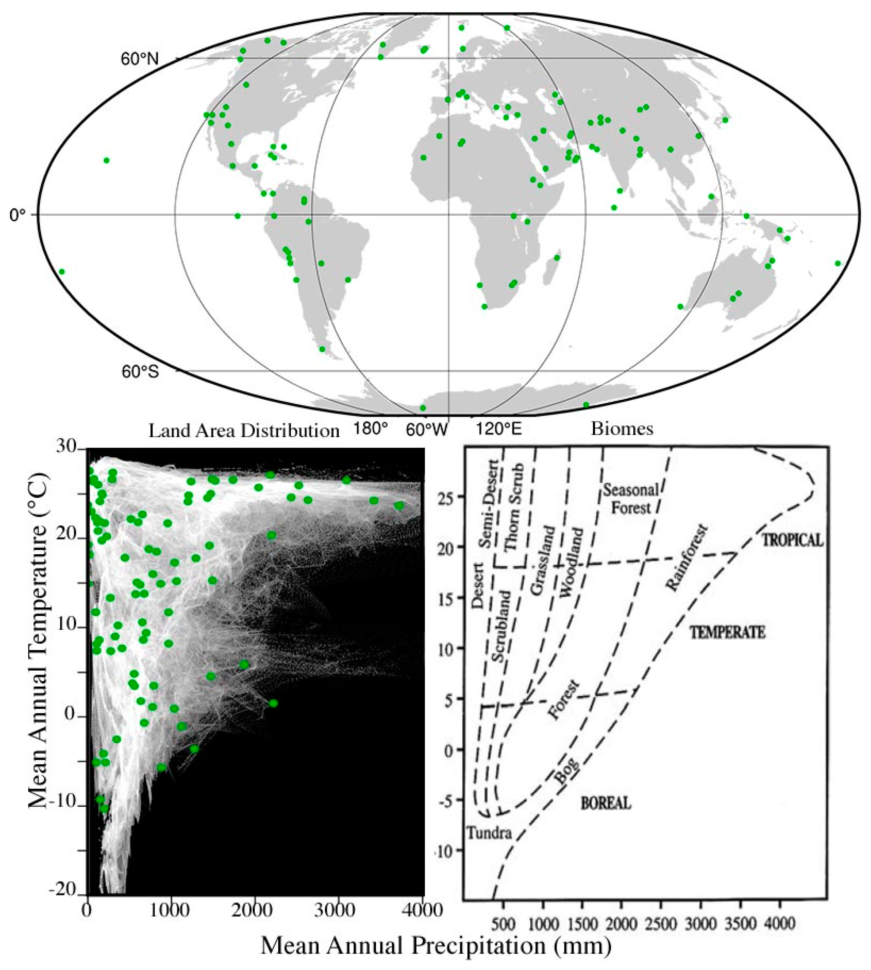
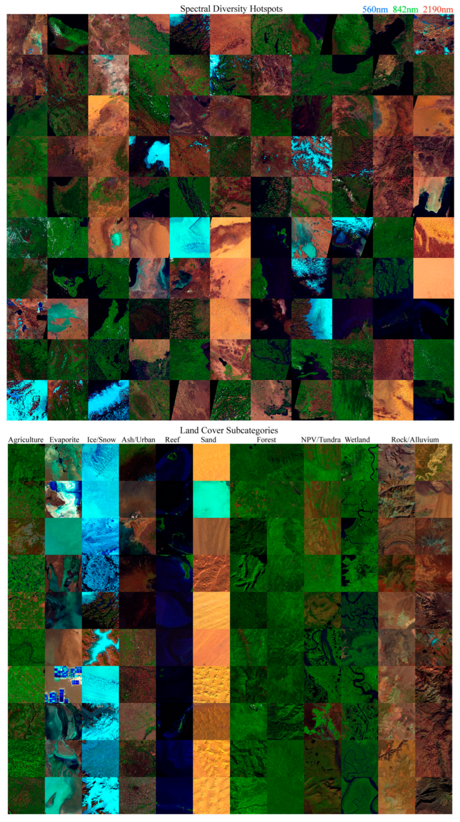
We construct a composite mixing space from a set of 110 Sentinel 2 MSI tiles collected from spectral diversity hotspots worldwide. The geographic locations and biome designations of these hotspots are shown in Figure 1. Unlike previous studies, we include numerous examples of cryospheric landscapes, evaporite basins and shallow marine environments, in addition to a range of anthropogenically modified landscapes (e.g., urban & agriculture). From this collection of (110 tiles × 10,9802 pixels =) 13.3 × 10⁹ Sentinel 2 spectra we identify a second set of (12 categories × 10 examples =) 120 subtiles from specific land cover subcategories. Diverse sets of either 5 or 10 subtiles, each 10 × 10 km in area, are chosen from agricultural (10), evaporite (10), cryospheric (10), volcanic (5), urban (5), shallow marine (10), sand dune (10), closed (10) and open (10) canopy forest, scrub/shrub (5), tundra (5), wetland (10), and igneous/sedimentary/metamorphic rock + alluvium (10 + 10) landscapes for a total 120,000,000 subcategory-specific spectra. False color composites of both of these aggregate mosaics are shown in Figure 2. Tile IDs and subcategory subtile locations are given in Appendix B. All data were downloaded free-of-charge as Level 1C exoatmospheric reflectance from the USGS EarthExplorer data portal (https://earthexplorer.usgs.gov/, accessed on 1 October 2022).
The spectral diversity hotspots were chosen on the basis of climatic gradients, biome diversity, soil diversity, plant diversity and geologic diversity—both within and among individual tiles. Sources used include geologic (https://mrdata.usgs.gov/geology/world/map-us.html, accessed on 11 September 2021) and climatic (https://storymaps.arcgis.com/stories/61a5d4e9494f46c2b520a984b2398f3b, accessed on 11 September 2021) basemaps in conjunction with maps of soils (https://atlas-for-the-end-of-the-world.com/world_maps/world_maps_soils.html, accessed on 11 September 2021), biomes (https://www.worldwildlife.org/publications/terrestrial-ecoregions-of-the-world, accessed on 11 September 2021), plant biodiversity (https://databasin.org/datasets/43478f840ac84173979b22631c2ed672/, accessed on 11 September 2021) and crop wild relatives (https://colostate.pressbooks.pub/cropwildrelatives/chapter/introduction-to-crop-wild-relatives/, accessed on 11 September 2021).
2.2. Methods
All analyses described in this study use Sentinel 2 MSI bands 1, 2, 3, 4, 5, 6, 7, 8, 8a, 11, and 12. The 20 m and 60 m bands (1) are coregistered with and upsampled to the 10 m bands (2, 3, 4, 8) by bilinear interpolation.
The compilation of 13.3 × 10⁹ Sentinel 2 spectra from 110 spectral diversity hotspots provides a basis for statistical assessment of the information content of the MSI spectral bands. The parametric Pearson correlation coefficient and the non-parametric Mutual Information metric were computed for all band pairs. The Pearson correlation coefficient, rxy, is given as:
where x and y are band-specific reflectances for each spectrum in the mosaic. Correlations are computed for all 55 band pairs.
The mutual information metric, as originally conceived by [16] and further formalized [17], is defined for two random variables X and Y as the Kullback–Leibler divergence from the product of the joint distribution from the product of the marginal distributions. That is,
where MI is mutual information, DKL is the Kullback–Leibler divergence, pX,Y is the joint distribution of X and Y, and pX and pY are the marginal distributions of X and Y. The MI of a variable with itself is defined as its self-information. Both mutual and self-information are bounded by [0, +], and MI SI. Conceptually, both self-information and MI can be understood as measures of “surprise”—the less probable are more surprising than probable events, and events with 100% probability are totally “unsurprising” (information = 0). Computation of MI was performed in Python using scikit-learn (package sklearn.featureselection.mutual_info_regression, with the implementation of [18,19]). As with the correlations, MI is computed for all 55 band pairs.
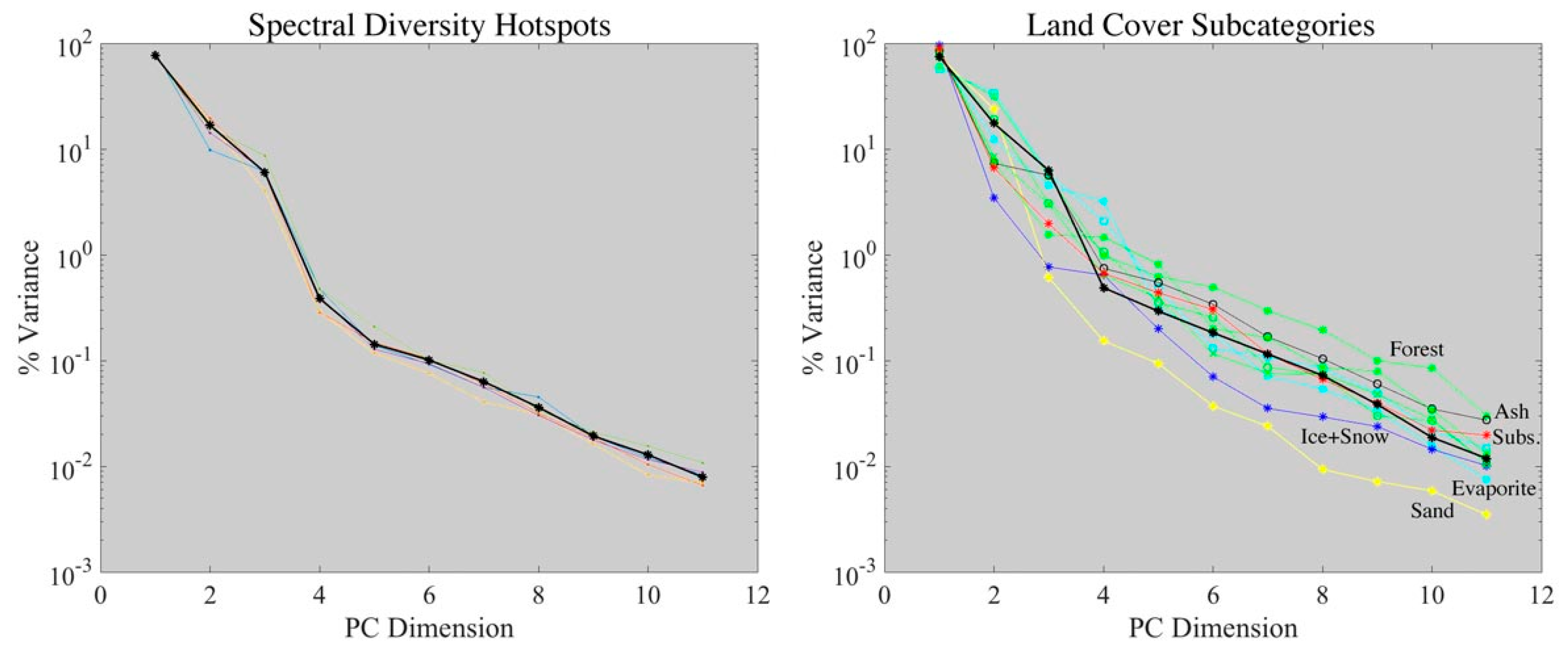
Spectral dimensionality is estimated from the variance partition of the eigenvalues of the spectra in the compilation mosaics described above. Variance partition by principal component dimension, given by the sum-normalized eigenvalues of the Singular Value Decomposition of the mosaics, and land cover subcategories, are shown in Figure 3. Because the tiles in the 120 tile spectral diversity hotspot mosaic are arranged in alphabetical order of the tile IDs (effectively random geographically), and most tiles are internally spectrally diverse, the mosaic can be subdivided into 5 subsets to assess the scaling of the spectral dimensionality of the compilation with number of spectra. Spectral dimensionality is estimated from variance partition for both the 110 tile Spectral Diversity Hotspot mosaic and the 120 subset land cover subcategory mosaic.
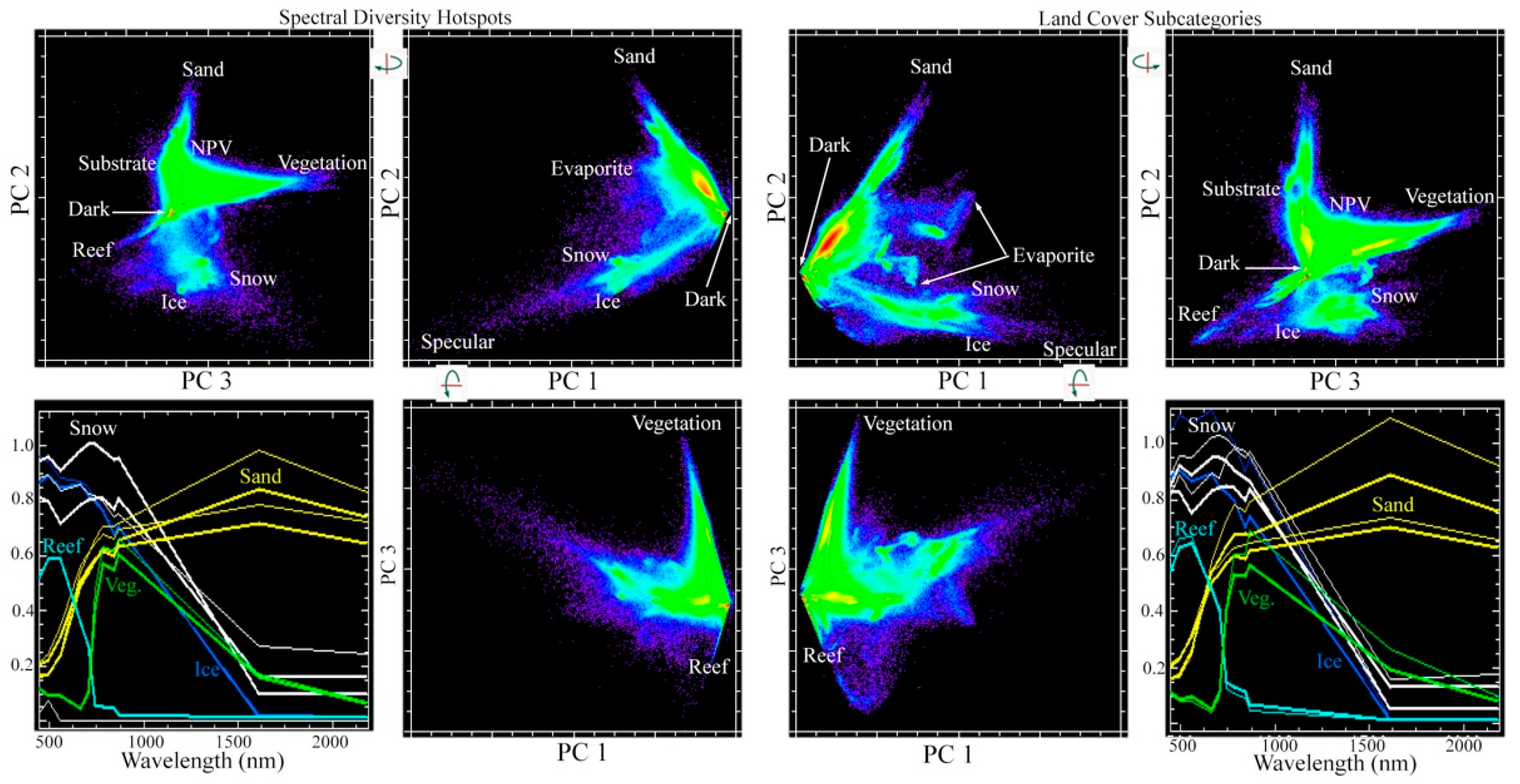
The topology of the Sentinel 2 MSI spectral mixing space is characterized with the low order principal components identified by the variance partition. As described by [20], apexes of the mixing space indicate spectral endmembers and straight edges between apexes indicate binary mixing lines between the corresponding endmembers. Three pairwise combinations of the three low order PCs provide orthogonal planar projections of the 3D mixing space. Because the PC transform maximizes variance partition into the smallest number of uncorrelated dimensions, it reveals the “global” structure of the mixing space corresponding to differences in the shape of the spectral continuum of different endmembers. Therefore, different categories of land cover with physical properties form distinct limbs on the mixing space.
An alternative approach can be provided by manifold learning. Here, “local” structure is revealed by a nonlinear mapping of high-dimensional spectra into lower-dimensional embedding space. This mapping is constructed in such a way to optimally preserve local (statistical “nearest neighbor”) distance and/or connectivity structures. In this analysis we use the Uniform Manifold Approximation and Projection (UMAP) algorithm [21] to provide a complementary projection for comparison to the PC-derived mixing space. The UMAP algorithm assumes that the Sentinel-2 spectra are uniformly distributed on a locally connected Riemannian manifold with an (approximately) locally constant Riemannian metric. UMAP models this manifold using a fuzzy topological structure, then seeks a low-dimensional (2- or 3-D) embedding with an optimally similar fuzzy topological structure. In general, the resulting embedding is nonlinear and not invertible. For excellent background information on UMAP, see: https://umap-learn.readthedocs.io/en/latest/ (accessed on 1 October 2022).
All UMAP computations were performed using the open source umap-learn Python package on a commercially available laptop computer with 32 GB RAM, 2GHz Quad-Core Intel Core i5 CPU, and a 1536 MB Intel Iris Plus Graphics GPU. Hyperparameter sensitivity was investigated by sweeps which looped through various choices of n_components, n_neighbors, and min_dist. Results were found to be relatively insensitive to all three hyperparameters, within at least 2 orders of magnitude of variability. All UMAP shown in this analysis used n_components = 2, n_neighbors = 5 or 500, and min_dist = 0.1.
Spectral EMs derived from the composite spectral mixing space provide the basis for the standardized SVD model, which is inverted to provide endmember fraction estimates for all spectra in the mosaic. The 3 EM linear spectral mixture model is given explicitly as a set of 11 band-specific mixing equations. Because the number of mixing equations exceeds the number of unknown fractions, the system is overdetermined, allowing for inversion by minimization of model misfit.
where E is the 3 column matrix of 11-band endmember vectors, O is the observed spectral vector to be modeled, FS|V|D is the vector of endmember fractions to be estimated, and ε is the model misfit to be minimized by the inversion. In addition, a unit sum constraint equation is included. The least squares solution, F = (ETE)−1ET O [22] for the S,V,D endmember fraction estimates gives fractions well-bounded [0, 1]. Model validity is assessed by the Root Mean Square (RMS) of the difference between observed and modeled spectra using the S, V, D estimates and endmember spectra in the forward model (L2 norm).
| FSE1 + FVE1 + FDE1 O1 |
| . . . |
| . . = . In matrix notation: O = FE + ε |
| . . . |
| FSE11 + FVE11 + FDE11 O11 |
3. Results
Information content of the Sentinel 2 MSI bands is quantified using both Pearson’s r parametric correlation and the mutual information (MI) metric for all 55 band pairs for the 8 × 10 land cover subcategory mosaic. Table 1 and Table 2 give the r and MI matrices for each band pair for the 80 tile subset. In both matrices, values ≥ 0.8 are shown in bold italic. As in previous studies, the highest correlations occur between adjacent bands within the visible, near infrared (NIR) and shortwave infrared (SWIR) wavebands. However, unlike the study of [12] which focused only on soils and agriculture, this analysis also finds high correlations between visible and SWIR bands as a result of the high albedo sands included in the mosaic. The mutual information matrix shows a similar pattern of higher MI between adjacent band pairs within wavebands, but more pronounced than for r. In comparing correlations and MI estimates for all 55 band pairs, the two metrics show a decidedly nonlinear relationship, with a correlation of 0.88 and MI of 1.195 (r on MI) and 1.16 (MI on r) (Appendix A).
The spectral dimensionality of both the 110 tile spectral diversity hotspot mosaic and the 120 subset land cover subcategory mosaic are nearly identical (Figure 3), suggesting that the subcategories chosen encompass the salient structure of the larger spectral diversity hotspot mosaic. The variance partition in Figure 3 indicates that both mosaics are effectively 3D, containing 99% and 98% of spectral variance in the three low order dimensions and <<1% variance in all higher order dimensions. Figure 3 also shows the variance partition of 5 subsets of 20 tiles each, compared to the variance partition of the full 110 tile spectral diversity hotspot mosaic. The fact that all 5 subsets have nearly identical variance partition to the full mosaic suggests that each is sufficiently spectrally diverse to encompass the diversity of the full spectral mixing space. The implication of this convergence is that the full 110 tile mosaic is more than sufficient to encompass full global spectral diversity. Figure 3 also shows the variance partition of each of the 12 land cover subcategories compared to the variance partition of the full mosaic. As expected, there is significant variation among the subcategories with more homogeneous land cover like snow and sand showing lower relative dimensionality and others like evaporites showing higher relative dimensionality.
The topology of the spectral mixing spaces of both mosaics are very similar and consistent with their spectral dimensionality. Figure 4 shows the 3D mixing spaces of the 110 tile Spectral Diversity Hotspot mosaic and the 120 subset land cover subcategory mosaic as orthogonal projections of bivariate PC distributions, along with the most conspicuous spectral endmembers from each. Both mixing spaces show complete mixing continua spanning the Substrate, Vegetation and Dark endmembers (PC 3 vs. 2 projections)—although the greatest spectral variance is associated with the PC 1 vs. 2 projection, driven by the strong contrast of the two highest albedo endmembers, sand and snow. Snow/ice and reefs each form distinct mixing continua with the Dark endmember, while evaporites form more distinct clusters without a single dominant mixing continuum. This suggests a more complex spectral continuum that may not be as linear as the others. It is noteworthy that neither reefs nor evaporites generally represent linear spectral mixing among distinct land cover types. Whereas aggregate albedo of most landscapes is modulated by a combination of reflectance, illumination flux density and shadow, the albedo of reefs is also strongly influenced by water depth while the albedo of evaporite basins is most strongly modulated by moisture content and the presence of standing water. Purely cryospheric environments are distinguished from other environments by their more homogeneous gradients spanning the snow-firn-ice continuum. Partial snow cover in non-cryospheric environments (e.g., boreal forests) may exhibit linear or nonlinear spectral mixing, but is sufficiently complex to warrant a more focused investigation separately.
Because reefs, evaporite basins and cryospheric environments are geographically and spectrally distinct from the SVD continuum that encompasses the majority of Earth’s biomes, the focus of the rest of the analysis is on the 8 × 10 column subset of the land cover subcategories spanning the SVD continuum. This mixing space is effectively 2D with (81% + 14% =) 95% of variance in the two low order PC dimensions. This triangular mixing space is dominated by the Substrate-Dark and Vegetation-Dark mixing continua as seen in Figure 5. Unlike previous studies, the Sentinel 2 MSI SVD space shows a clear distinction (kink & discontinuity) between high albedo sands and the lower albedo substrates that bound one side of the SVD continuum. Most non-forest biomes fall within this continuum, with varying amounts of nonphotosynthetic vegetation (NPV) and exposed substrate interspersed with herbaceous and woody photosynthetic vegetation.
The Substrate limb discontinuity, combined with the diffuse apex of the Vegetation limb suggest two different, but related, SVD models. Because pure sands (e.g., dunefields) rarely support vegetation communities, an SVD model using an inner Substrate endmember (Si) is more physically plausible than an SVD model using an outer Substrate endmember (So) composed of pure sand. However, the outer Substrate endmember could be used for modeling landscapes where bright sands are prominent. Similarly, an outer Vegetation endmember (Vo) composed of a single pixel spectrum is less representative than an inner Vegetation endmember (Vi) composed of an average of several individual spectra at the more densely occupied inner Vegetation apex of the mixing space. Comparisons of inner and outer S and V endmembers are shown in Figure 5. All 5 endmember spectra are given in Table 3.
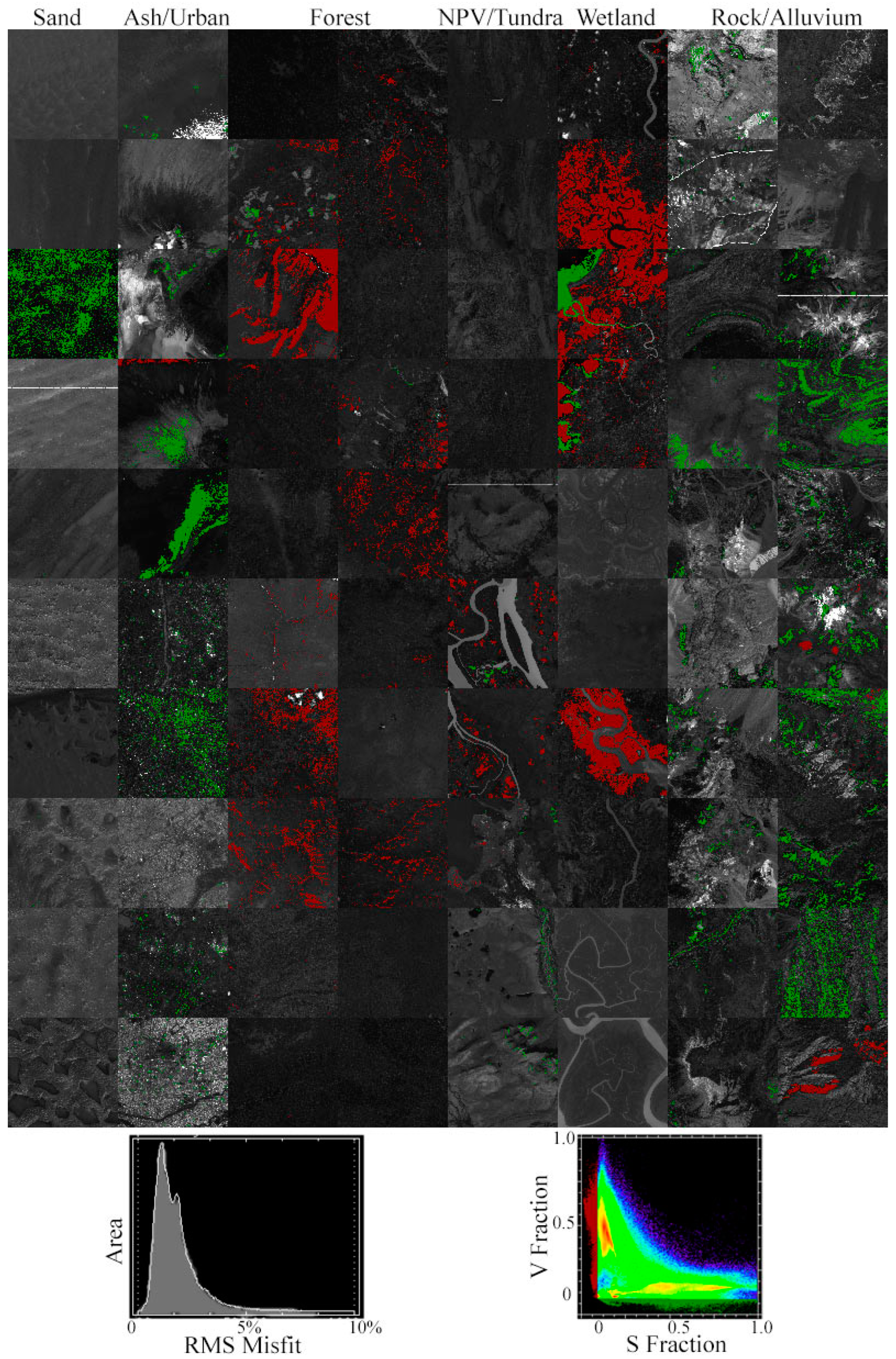
Inversion of the SVD linear mixture model using the inner Si and Vi endmembers yields the SVD fraction space shown in Figure 5. As expected, S fractions for the high albedo sands outside the triangular model exceed 1.0 with Dark fractions <0, but all other fraction estimates are well-bounded [0, 1]. Relatively small percentages of the binary S-D and V-D mixtures have V and S (respectively) fractions are slightly negative, but almost all are within 5% of 0. As shown in Figure 6, the spectra with these slightly negative near-zero fractions are limited to a few spatially contiguous geographies (e.g., mangroves, dunes or volcanic ash deposits). The distribution of RMS misfit between the observed and modeled spectra for the 80 subcategory composite has <6% misfit for >99% of 80,000,000 Sentinel 2 spectra, with the upper tail of higher misfits also limited to a few specific land covers not represented in the SVD model (e.g., turbid water, evaporites and light snow).
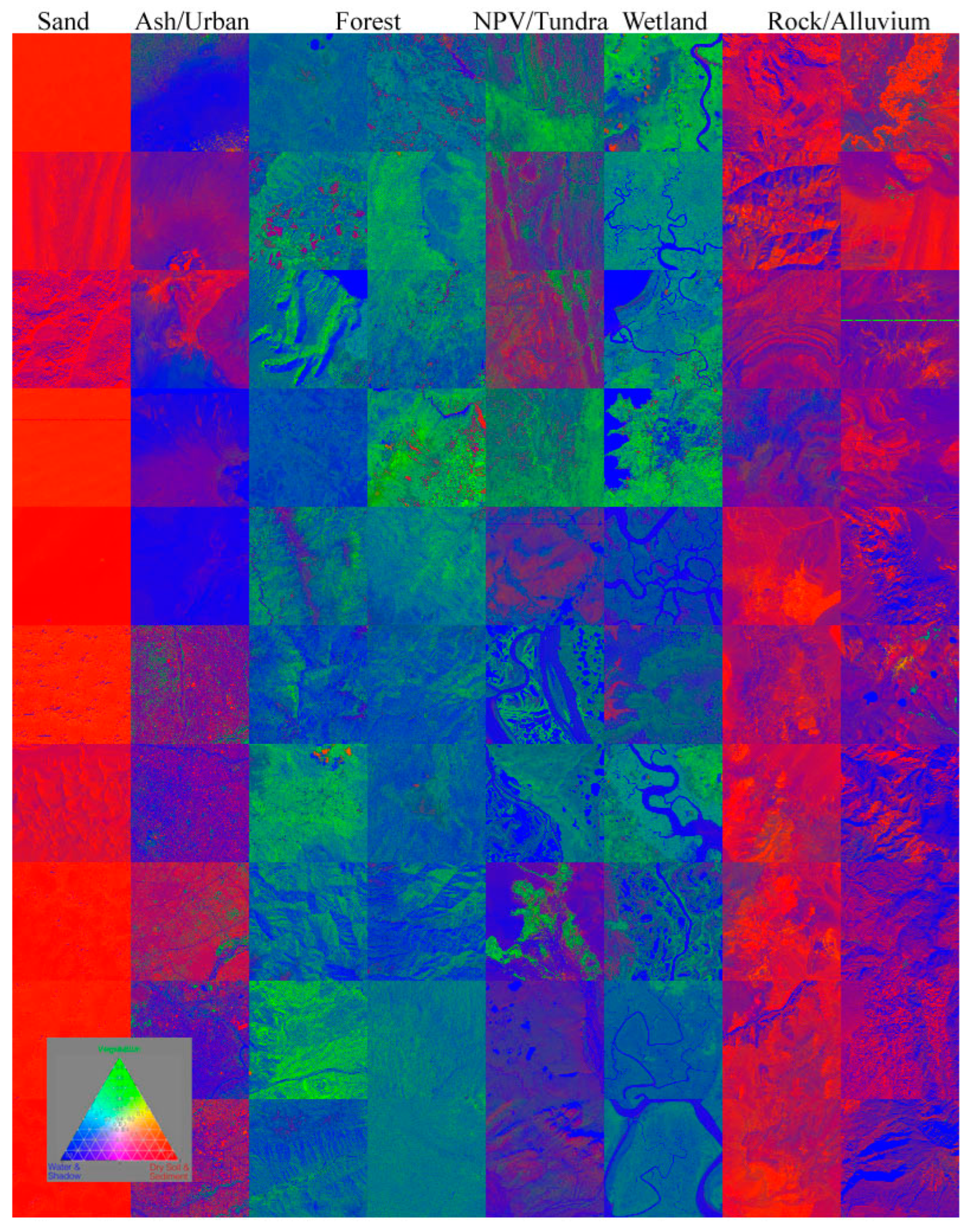
The SVD fraction composite for the 8 × 10 land cover subcategories (Figure 7) is skewed toward RGB primaries, consistent with the S-D and V-D binary mixing continua seen in the SVD mixing space. The larger, more spatially heterogeneous collection of 110 spectral diversity hotspot tiles shows a wider range of intermediate spectral mixtures, as would be expected.
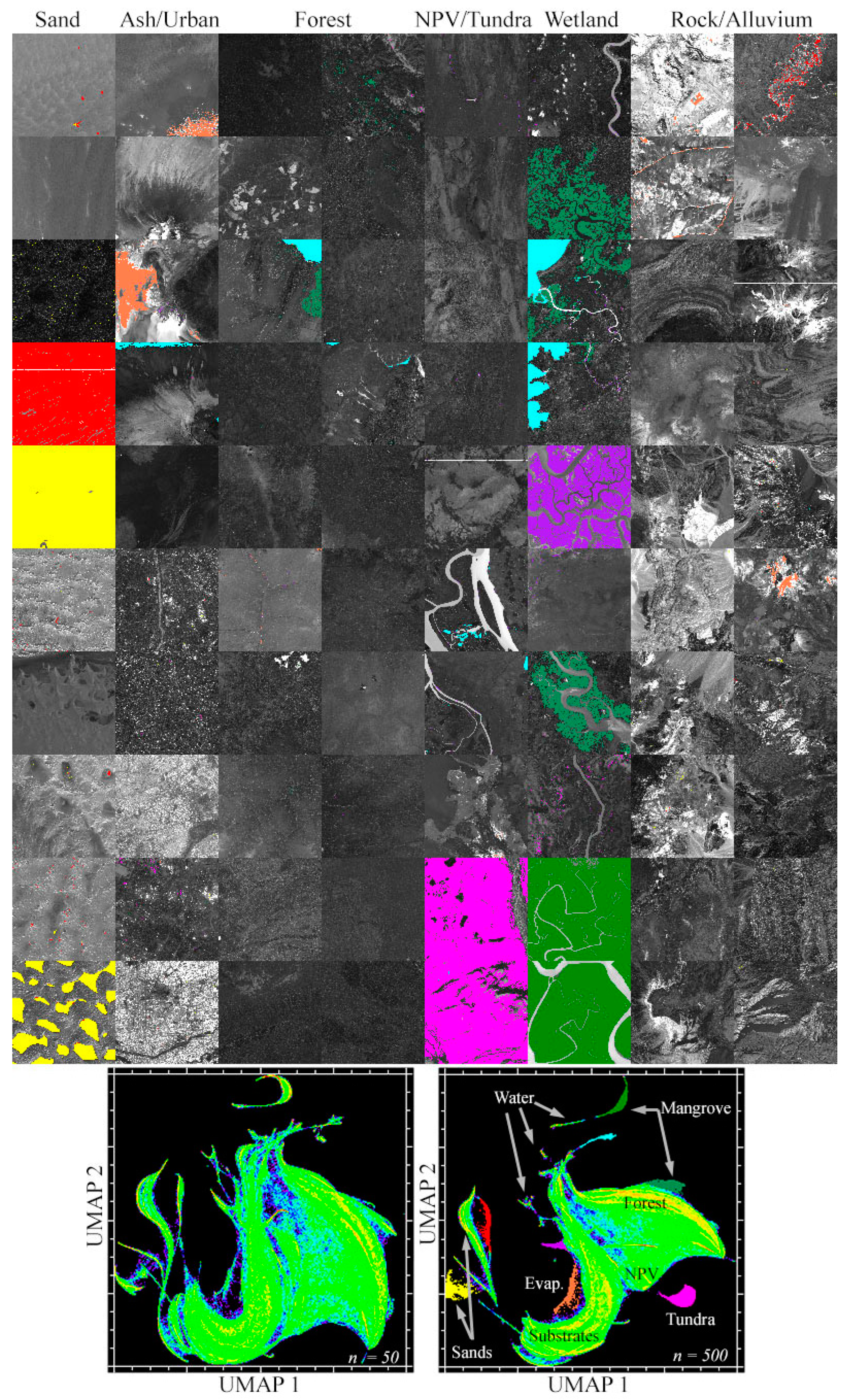
The spectral mixing space rendered by the 2D UMAP embedding preserves the binary S-D and V-D mixing trends that dominate the PC and fraction spaces. Figure 8 shows a broader mixing continuum for the V-D limb extending to NPV-dominant biomes near the distinct S-D continuum. However, both UMAP embeddings also show a number of distinct clusters located outside the S-D and V-D continua. Most obvious are the several distinct sand clusters associated with different dunefields with distinct sand mineralogies. Additionally, noteworthy are the single distinct clusters associated with two tundra sites in the Canadian and Alaskan arctic and the single cluster associated with two mangrove sites in the Bangladesh Sundarban. It is noteworthy that all of the distinct clusters are associated with specific, spatially contiguous, areas within individual (sometimes multiple) subsets that are evident when labeled clusters in the UMAP space are back-projected to geographic space.
4. Discussion
4.1. Spectral Information Content
The increased NIR spectral resolution of the Sentinel 2 MSI sensors contributes substantially to the spectral information content. While the correlations of adjacent spectral bands within the visible, NIR and SWIR are >0.8, scatterplots of band pairs reveal conspicuous departures from linearity in all but the highest correlations (>~0.95) which are reflected in correspondingly lower MI scores. A comparison of all bands with MSI band 8 in Appendix A illustrates a variety of such features, suggesting a diversity of spectra with significantly different reflectance (e.g., absorptions) between adjacent spectral bands. As in previous studies using Landsat multispectral and AVIRIS hyperspectral, the primary correlation structure clearly distinguishes visible, NIR and SWIR wavebands [12], but both r and MI suggest only moderate redundancy between adjacent spectral bands within each waveband. This may be partially responsible for the two clearly diverging lower limbs of the V-D continuum (Fv < ~0.5) trending toward the Dark endmember and toward the ternary mixing NPV + soil + shadow region near the S-D mixing continuum. Empirically, these mixing trends appear to correspond to closed and open canopy forest. Figure 5 also shows two distinct subparallel clusters on a single mixing trend on the V-D mixing continuum in the PC 3 vs. 2 space. These features are not seen in either the Landsat or MODIS mixing spaces [7,8].
Among the new VNIR bands provided by Sentinel 2 MSI, the greatest redundancy appears to be among bands 7, 8 and 8a, as indicated by some of the highest MI values. Whereas bands 4 and 5 have a correlation of 0.99, their MI is a comparatively lower 1.03, suggesting that the MI metric can resolve nonredundancies that correlation does not. The curvature of the log-linear relationship between the upper tails of the r and MI relationship (Appendix A) suggests that the two metrics are sensitive to different disparities between band reflectance distributions. Given the wide diversity of reflectances included in these mixing spaces, the similarities and differences in spectral continuum shape may overshadow meaningful differences in VNIR band information content. The fact that the UMAP embeddings identify a number of distinct clusters and apexes not apparent in the PC-derived feature space suggests that subtle differences in continuum curvature captured by the narrow NIR bands may indeed provide potentially useful resolving power to discriminate between otherwise similar reflectances within land cover subcategories.
4.2. Spectral Dimensionality and Mixing Space Topology
While the full mixing spaces shown in Figure 4 are both 3D, neither is amenable to a single mixture model containing 6+ endmembers (SVD + evaporite, reef, snow/ice). Such a mixture model would be both physically and mathematically implausible. Physically, as discussed above, reefs, evaporite basins and cryospheric landscapes are generally distinct from the continuum of biomes (Figure 1) in which a substrate continuum is interspersed with multiple scales of photosynthetic and nonphotosynthetic vegetation and structural shadow. Mathematically, the similarity of spectral shape of many evaporites with ice and snow spectra, and the inverse similarity of both to vegetation spectra will destabilize any inversion containing either two or all three of these endmembers because they are far from orthogonal, and often nearly colinear. The result is significant percentages of strongly negative (<−0.5) fractions in one or more of the fraction distributions. These are the primary reasons we focus on the 8 × 10 subset mosaic and the SVD model for the latter part of this analysis.
4.3. The SVD Model
The new, lower amplitude, Substrate endmember identified from the break in the S-D continuum supports a more physically plausible mixture model than earlier SVD models which used sand spectra for the Substrate EM. Using high albedo sand as an endmember has the undesirable consequence of likely underestimating the true substrate fraction in most situations where sand is not actually present. While we have advocated the use of local Substrate endmembers in previous studies, we find the use of a more realistic standardized Substrate reflectance as a reasonable substitute in situations where a single local Substrate endmember cannot be identified. In many landscapes, a more distinct plane of substrates may be more apparent than in the mixing spaces of these unusually diverse collections of spectra. If so, local soil and NPV endmembers might be distinguishable, as we have found in similar analyses of compilations of hyperspectral data in agricultural environments [13]. Because we did not identify a distinct apex associated with NPV in either of the composite mixing spaces, and observe that NPV occupies an intermediate region on the Substrate-Dark mixing continuum, we find no reason to extend the SVD model to include a NPV endmember.
The use of a lower amplitude inner Substrate endmember also provides more dynamic range to the Substrate fraction distribution by eliminating the much brighter sands which compress the dynamic range of the Substrate fraction. Allowing greater dynamic range may also facilitate distinction between different dry soil reflectances and different moisture content within a single soil type. At present, variations in dry reflectance and variations in moisture content are accommodated by varying fractions of Dark endmember—representing a fundamental ambiguity in the SVD model specifically and broadband reflectance generally. While this distinction may be impossible in single date imagery, spatiotemporal variations in soil moisture (and hence the S-D fraction continuum) of a single location may facilitate distinguishing these two effects on soil reflectance.
4.4. Manifold Topology and Spectral Resolution
The use of nonlinear, nonparametric dimensionality reduction provides a new and potentially very useful approach to spectral feature/mixing space characterization [23]. The presence of numerous distinct clusters in the UMAP projections contrasts strongly to the much more continuous PC-derived feature spaces. While the latter are essential to identifying spectral endmembers and verifying linearity of spectral mixing, the variance maximization on which the PC transform is based is much more sensitive to the shape of the spectral continuum than the presence of more subtle (lower variance) absorption features. In contrast, manifold learning algorithms that preserve local structure in the form of nearest neighbor proximity (e.g., UMAP, t-SNE) make it possible to identify more subtle differences in spectral curvature and absorption features (often aliased in multispectral imagery) that convey real physical meaning and may considerably extend the usable information content of narrowband multispectral sensors like Sentinel 2 MSI. The companion study to this [24] carries this duality a step further by combining the physically interpretable structure of the SVD mixing space with the more subtle features of local scale manifolds in the form of a joint characterization of the spectral mixing space.
In summary, the construction of a diverse collection of Sentinel 2 MSI tiles from 110 spectral diversity hotspots worldwide provides a basis for a globally representative spectral feature space. Because spectral mixing is pervasive in most biomes, even at 10 m resolution, we refer to this aliased feature space as a spectral mixing space. Identification of more spectrally homogeneous examples of a variety of specific land cover subcategories makes it possible to separate landscapes dominated by nonlinear spectral mixing (reefs, evaporite basins and cryospheric landscapes) from the more linear SVD continuum that spans most terrestrial biomes. Global standardized SVD endmembers chosen from the inner apexes of the SVD mixing space provide the basis for a general model of fractional subpixel land cover that is applicable to most biomes. While the PC-based mixing space allows for unambiguous identification of spectral endmembers, and determination of linearity of mixing (and inversion of linear mixture models), the use of nonlinear manifold learning to project proximity-preserving embeddings of the higher dimensional mixing space allows for identification of both mixing continua and isolated clusters of spectrally distinct land covers that are not generally apparent in the PC-based mixing space.
Author Contributions
Conceptualization, C.S. and D.S.; methodology, C.S. and D.S.; writing and editing, C.S. and D.S. All authors have read and agreed to the published version of the manuscript.
Funding
DS gratefully acknowledges funding from the USDA NIFA Sustainable Agroecosystems program (Grant # 2022-67019-36397), the NASA Land-Cover/Land Use Change program (Grant # NNH21ZDA001N-LCLUC), the NASA Remote Sensing of Water Quality program (Grant # 80NSSC22K0907), and the NSF Signals in the Soil program (Award # 2226649). CS acknowledges the support of the endowment of the Lamont Doherty Earth Observatory.
Data Availability Statement
The data supporting this manuscript can be downloaded free of charge from the web portals listed in the main text.
Acknowledgments
We are grateful to the three anonymous reviewers for help comments and suggestions.
Conflicts of Interest
The authors declare no conflict of interest.
Appendix A. Correlation and Mutual Information
Figure A1.
Correlation vs. Mutual Information estimates and band to band bivariate distributions for the 80 land cover specific subset mosaic. For all band to band pairs (top) correlation and Mutual Information estimates show a correlation of 0.88 and MI of 1.195 (r on MI) and 1.16 (MI on r), with some degree of Log-linear scaling on the lower tail of the distribution and clear nonlinearity on the upper tail. The range of both metrics suggests that almost all non-adjacent, and some adjacent, band combinations provide some discriminative utility for at least some land cover subcategories. Bivariate distributions of MSI band 8 with all other bands show considerable deviations from linearity for all but band 7.

Appendix B

Table A1.
Sentinel 2 tileIDs.
| c1 | c2 |
| S2A_MSIL1C_20160723T143750_T19KEQ | S2A_MSIL1C_20170205T210921_N0204_R057_T04QHH |
| S2A_MSIL1C_20160723T143750__T19KER | S2B_MSIL1C_20180311T185149_N0206_R113_T10SFJ |
| S2A_MSIL1C_20170118T081241_N0204_R078_T35MRV | S2A_MSIL1C_20170315T101021_N0204_R022_T32TPP |
| S2A_MSIL1C_20170119T074231_N0204_R092_T36JTT | S2A_MSIL1C_20170412T074611_N0204_R135_T37PDQ |
| S2A_MSIL1C_20170119T074231_N0204_R092_T36JUT | S2A_MSIL1C_20170427T021921_N0205_R060_T50HLH |
| S2A_MSIL1C_20170119T143731_N0204_R096_T20NNM | S2A_MSIL1C_20170427T153621_N0205_R068_T18NTP |
| S2A_MSIL1C_20170124T051101_N0204_R019_T43PGL | S2A_MSIL1C_20170428T215921_N0205_R086_T01KFS |
| S2A_MSIL1C_20170124T051101_N0204_R019_T44RQV | S2A_MSIL1C_20170506T054641_N0205_R048_T42QXM |
| S2A_MSIL1C_20170124T165551_N0204_R026_T14QQE | S2A_MSIL1C_20170508T012701_N0205_R074_T54STE |
| S2A_MSIL1C_20170125T202521_N0204_R042_T58CDU | S2A_MSIL1C_20170604T043701_N0205_R033_T45RYL |
| c3 | c4 |
| S2A_MSIL1C_20170613T182921_N0205_R027_T11SMB | S2A_MSIL1C_20170723T064631_N0205_R020_T41TKG |
| S2A_MSIL1C_20170620T181921_N0205_R127_T12TTK | S2A_MSIL1C_20170723T182921_N0205_R027_T11UQQ |
| S2A_MSIL1C_20170621T074941_N0205_R135_T37RGL | S2A_MSIL1C_20170724T145731_N0205_R039_T18LZL |
| S2A_MSIL1C_20170627T180911_N0205_R084_T12SUF | S2A_MSIL1C_20170830T125301_N0205_R138_T27WXM |
| S2A_MSIL1C_20170627T180911_N0205_R084_T12SUG | S2A_MSIL1C_20170830T131241_N0205_R138_T23KLP |
| S2A_MSIL1C_20170628T173901_N0205_R098_T13SCS | S2A_MSIL1C_20170908T063621_N0205_R120_T40QFK |
| S2A_MSIL1C_20170704T013711_N0205_R031_T52MHD | S2A_MSIL1C_20170914T065621_N0205_R063_T40TFQ |
| S2A_MSIL1C_20170705T022551_N0205_R046_T50NMN | S2A_MSIL1C_20170915T213531_N0205_R086_T06WVS |
| S2A_MSIL1C_20170718T210021_N0205_R100_T08WNB | S2A_MSIL1C_20170916T055631_N0205_R091_T42RUN |
| S2A_MSIL1C_20170719T084601_N0205_R107_T41XNE | S2A_MSIL1C_20170917T190351_N0205_R113_T10SFG |
| c5 | c6 |
| S2A_MSIL1C_20170919T142931_N0205_R139_T23VMH | S2A_MSIL1C_20171117T064141_N0206_R120_T40RFU |
| S2B_MSIL1C_20180328T183949_N0206_R070_T11SKA | S2A_MSIL1C_20171129T142031_N0206_R010_T18FXJ |
| S2A_MSIL1C_20170923T074231_N0205_R049_T37PHN | S2A_MSIL1C_20171201T150711_N0206_R039_T18LZH |
| S2A_MSIL1C_20171002T150621_N0205_R039_T19LBE | S2A_MSIL1C_20171203T034121_N0206_R061_T48QUM |
| S2A_MSIL1C_20171003T143321_N0205_R053_T20MQC | S2A_MSIL1C_20171207T082321_N0206_R121_T34HCH |
| S2A_MSIL1C_20171013T080931_N0205_R049_T25CEM | S2A_MSIL1C_20171208T111441_N0206_R137_T29QKD |
| S2A_MSIL1C_20171016T073911_N0205_R092_T36MZC | S2A_MSIL1C_20171209T072301_N0206_R006_T38QND |
| S2A_MSIL1C_20171017T103021_N0205_R108_T32TLQ | S2A_MSIL1C_20171210T065251_N0206_R020_T40QCJ |
| S2A_MSIL1C_20171107T070231_N0206_R120_T39LUC | S2A_MSIL1C_20160615T183312_N0204_R127_T11SPS |
| S2A_MSIL1C_20171117T064141_N0206_R120_T40RFU | S2A_OPER_PRD_MSIL1C_PDMC_20150813T101657 |
| c7 | c8 |
| S2A_MSIL1C_20150813T101026_N0204_R022_T32UPU | S2A_OPER_MSI_L1C_TL_EPA__20161012T193400_A006777_T55KCB |
| S2A_MSIL1C_20151022T184002_N0204_R027_T11SMA | S2B_MSIL1C_20170713T023549_N0205_R089_T51RTN |
| S2A_OPER_PRD_MSIL1C_PDMC_20151206T145051 | S2B_MSIL1C_20170723T124309_N0205_R095_T28WDT |
| S2A_OPER_PRD_MSIL1C_PDMC_20160318T145513_01 | S2B_MSIL1C_20170727T053639_N0205_R005_T43SFV |
| S2A_OPER_MSI_L1C_TL_SGS__20161011T162433_A006812_T32WPT | S2B_MSIL1C_20170730T040549_N0205_R047_T47SND |
| S2A_OPER_MSI_L1C_TL_SGS__20161013T032322_A006834_T56LKR | S2B_MSIL1C_20170816T005709_N0205_R002_T53JQJ |
| S2A_OPER_MSI_L1C_TL_EPA__20161012T193400_A006777_T55LCC | S2B_MSIL1C_20170817T114639_N0205_R023_T33XWF |
| S2A_OPER_MSI_L1C_TL_MTI__20161014T211238_A006858_T15MXV | S2B_MSIL1C_20170824T145909_N0205_R125_T22WEV |
| S2A_OPER_MSI_L1C_TL_SGS__20161017T100159_A006894_T45QYG | S2B_MSIL1C_20170826T155519_N0205_R011_T17NMJ |
| S2A_OPER_MSI_L1C_TL_MTI__20161018T111609_A006910_T38RPV | S2B_MSIL1C_20170905T085549_N0205_R007_T35TMF |
| c9 | c10 |
| S2B_MSIL1C_20170906T002659_N0205_R016_T55KCA | S2B_MSIL1C_20171013T081959_N0205_R121_T36SYF |
| S2B_MSIL1C_20170912T084549_N0205_R107_T36TUL | S2B_MSIL1C_20171019T083959_N0205_R064_T36STF |
| S2B_MSIL1C_20170912T170949_N0205_R112_T14RLP | S2B_MSIL1C_20171101T004649_N0206_R102_T54JTL |
| S2B_MSIL1C_20170916T215519_N0205_R029_T06WVB | S2B_MSIL1C_20171103T061009_N0206_R134_T42SWC |
| S2B_MSIL1C_20170918T054629_N0205_R048_T43SDT | S2B_MSIL1C_20171103T061009_N0206_R134_T42SWD |
| S2B_MSIL1C_20170918T205119_N0205_R057_T07VEG | S2B_MSIL1C_20171116T132219_N0206_R038_T23KKP |
| S2B_MSIL1C_20170919T140039_N0205_R067_T21KVA | S2B_MSIL1C_20171123T043059_N0206_R133_T45QYE |
| S2B_MSIL1C_20170929T222959_N0205_R072_T60KWF | S2B_MSIL1C_20171130T160619_N0206_R097_T17RMH |
| S2B_MSIL1C_20171008T105009_N0205_R051_T30TYN | S2B_MSIL1C_20171202T064229_N0206_R120_T40RGU |
| S2B_MSIL1C_20171009T003649_N0205_R059_T55MDP | S2B_MSIL1C_20171207T105419_N0206_R051_T30RVT |
| c11 | |
| S2B_MSIL1C_20171208T052209_N0206_R062_T44SMD | |
| S2B_MSIL1C_20180729T141049_N0206_R110_T21LTC | |
| S2B_MSIL1C_20171208T084329_N0206_R064_T33JWN | |
| S2B_MSIL1C_20171212T064249_N0206_R120_T40QEL | |
| S2B_MSIL1C_20171212T064249_N0206_R120_T40QFH | |
| S2B_MSIL1C_20171212T100359_N0206_R122_T32RLQ | |
| S2B_MSIL1C_20180622T085559_N0206_R007_T34RGS | |
| S2B_MSIL1C_20171214T155519_N0206_R011_T18RUN | |
| S2B_MSIL1C_20171215T152629_N0206_R025_T18NUF | |
| S2B_MSIL1C_20171227T160459_N0206_R054_T17QME | |
Table A2.
TileIDs and NW corner coordinates of land cover subcategory subsets.
| Agriculture | |||
| TileID | UTM Zone | Easting | Northing |
| S2A_MSIL1C_20170205T210921_N0204_R057_T04QHH | 4N | 868610 | 2223190 |
| S2A_MSIL1C_20170315T101021_N0204_R022_T32TPP | 32N | 623950 | 4864330 |
| S2A_MSIL1C_20170508T012701_N0205_R074_T54STE | 54N | 269220 | 3988590 |
| S2A_MSIL1C_20170723T064631_N0205_R020_T41TKG | 41N | 266210 | 4645260 |
| S2A_MSIL1C_20170917T190351_N0205_R113_T10SFG | 10N | 688930 | 4167330 |
| S2A_OPER_PRD_MSIL1C_PDMC_20161017T044357 | 45N | 723470 | 2625060 |
| S2B_MSIL1C_20170730T040549_N0205_R047_T47SND | 47N | 554190 | 4363690 |
| S2B_MSIL1C_20170918T054629_N0205_R048_T43SDT | 43N | 459570 | 3800040 |
| S2B_MSIL1C_20171008T105009_N0205_R051_T30TYN | 30N | 702100 | 4787760 |
| S2B_MSIL1C_20171013T081959_N0205_R121_T36SYF | 36N | 778000 | 4095680 |
| Sand | |||
| TileID | UTM Zone | Easting | Northing |
| S2A_MSIL1C_20170628T173901_N0205_R098_T13SCS | 13N | 372290 | 3654900 |
| S2A_MSIL1C_20170908T063621_N0205_R120_T40QFK | 40N | 653400 | 2447190 |
| S2A_MSIL1C_20171119T040041_N0206_R004_T48TUK | 48N | 305540 | 4438710 |
| S2A_MSIL1C_20171208T111441_N0206_R137_T29QKD | 29N | 291550 | 2399280 |
| S2A_MSIL1C_20171209T072301_N0206_R006_T38QND | 38N | 527910 | 1890720 |
| S2B_MSIL1C_20171207T105419_N0206_R051_T30RVT | 30N | 481880 | 3290910 |
| S2B_MSIL1C_20171208T084329_N0206_R064_T33JWN | 33S | 541880 | 7265640 |
| S2B_MSIL1C_20171212T100359_N0206_R122_T32RLQ | 32N | 339750 | 2966720 |
| S2B_MSIL1C_20171212T100359_N0206_R122_T32RLR | 32N | 331950 | 3100020 |
| Lava & Ash | |||
| TileID | UTM Zone | Easting | Northing |
| S2A_MSIL1C_20170205T210921_N0204_R057_T04QHH | 4N | 861160 | 2206290 |
| S2A_MSIL1C_20171016T073911_N0205_R092_T36MZC | 36S | 819250 | 9703580 |
| S2A_MSIL1C_20171016T073911_N0205_R092_T36MZC | 36S | 834220 | 9768640 |
| S2A_OPER_PRD_MSIL1C_PDMC_20161014T163303 | 15S | 652170 | 9967520 |
| S2B_MSIL1C_20170723T124309_N0205_R095_T28WDT | 28N | 399960 | 7200220 |
| Urban | |||
| TileID | UTM Zone | Easting | Northing |
| S2A_MSIL1C_20170508T012701_N0205_R074_T54STE | 54N | 269890 | 3950620 |
| S2A_MSIL1C_20170830T131241_N0205_R138_T23KLP | 23S | 328970 | 7398470 |
| S2A_MSIL1C_20170916T055631_N0205_R091_T42RUN | 42N | 300000 | 2758120 |
| S2A_MSIL1C_20171017T103021_N0205_R108_T32TLQ | 32N | 390060 | 4999690 |
| S2B_MSIL1C_20170912T170949_N0205_R112_T14RLP | 14N | 364980 | 2848280 |
| Forest—1 | |||
| TileID | UTM Zone | Easting | Northing |
| S2A_MSIL1C_20170118T081241_N0204_R078_T35MRV | 35S | 831290 | 9963030 |
| S2A_MSIL1C_20170119T074231_N0204_R092_T36JTT | 36S | 284150 | 7247210 |
| S2A_MSIL1C_20170205T210921_N0204_R057_T04QHH | 4N | 847400 | 2230620 |
| S2A_MSIL1C_20170427T021921_N0205_R060_T50HLH | 50S | 355240 | 6230970 |
| S2A_MSIL1C_20170508T012701_N0205_R074_T54STE | 54N | 257880 | 3907290 |
| S2A_MSIL1C_20170604T043701_N0205_R033_T45RYL | 45N | 794940 | 3088140 |
| S2A_MSIL1C_20170705T022551_N0205_R046_T50NMN | 50N | 450950 | 704020 |
| S2A_MSIL1C_20170724T145731_N0205_R039_T18LZL | 18S | 875170 | 8546360 |
| S2A_MSIL1C_20170724T145731_N0205_R039_T19LBF | 19S | 215640 | 8582190 |
| S2A_MSIL1C_20170830T131241_N0205_R138_T23KLP | 23S | 321220 | 7348390 |
| Forest—2 | |||
| TileID | UTM Zone | Easting | Northing |
| S2A_MSIL1C_20170917T190351_N0205_R113_T10SFG | 10N | 607440 | 4106660 |
| S2A_OPER_PRD_MSIL1C_PDMC_20151206T145051 | 20N | 469370 | 431170 |
| S2B_MSIL1C_20170713T023549_N0205_R089_T51RTN | 51N | 231700 | 3257530 |
| S2B_MSIL1C_20170718T101029_N0205_R022_T32TQS | 32N | 773730 | 5121020 |
| S2B_MSIL1C_20170906T002659_N0205_R016_T55KCA | 55S | 353630 | 8006280 |
| S2B_MSIL1C_20170912T084549_N0205_R107_T36TUL | 36N | 335150 | 4512660 |
| S2B_MSIL1C_20171009T003649_N0205_R059_T55MDP | 55S | 469610 | 9317570 |
| S2B_MSIL1C_20171013T081959_N0205_R121_T36SYF | 36N | 791100 | 4092030 |
| S2B_MSIL1C_20171116T132219_N0206_R038_T23KKP | 23S | 215910 | 7344400 |
| S2B_MSIL1C_20171215T152629_N0206_R025_T18NUF | 18N | 381240 | 26200 |
| Senescent Vegetation | |||
| TileID | UTM Zone | Easting | Northing |
| S2A_MSIL1C_20170119T074231_N0204_R092_T36JUT | 36S | 387540 | 7237130 |
| S2A_MSIL1C_20170119T074231_N0204_R092_T36JUT | 36S | 381920 | 7259800 |
| S2A_MSIL1C_20170119T074231_N0204_R092_T36JUT | 36S | 375110 | 7261040 |
| S2A_MSIL1C_20170119T074231_N0204_R092_T36JUT | 36S | 379990 | 7209420 |
| S2A_MSIL1C_20170516T154911_N0205_R054_T18TWQ | 18N | 563770 | 4938390 |
| Tundra & Wetlands | |||
| TileID | UTM Zone | Easting | Northing |
| S2A_MSIL1C_20170718T210021_N0205_R100_T08WNB | 8N | 508380 | 7654750 |
| S2A_MSIL1C_20170718T210021_N0205_R100_T08WNB | 8N | 540940 | 7608620 |
| S2A_OPER_PRD_MSIL1C_PDMC_20160318T145513 | 19S | 495986 | 7997974 |
| S2B_MSIL1C_20170916T215519_N0205_R029_T06WVB | 6N | 442210 | 7700040 |
| S2B_MSIL1C_20170916T215519_N0205_R029_T06WVB | 6N | 458950 | 7676830 |
| Mangroves | |||
| TileID | UTM Zone | Easting | Northing |
| S2A_MSIL1C_20170427T153621_N0205_R068_T18NTP | 18N | 258620 | 824760 |
| S2A_MSIL1C_20170704T013711_N0205_R031_T52MHD | 52S | 814620 | 9839210 |
| S2A_MSIL1C_20170705T022551_N0205_R046_T50NMN | 50N | 498390 | 752360 |
| S2A_MSIL1C_20170705T022551_N0205_R046_T50NMN | 50N | 423780 | 704730 |
| S2A_MSIL1C_20170916T055631_N0205_R091_T42RUN | 42N | 319520 | 2736030 |
| S2A_OPER_PRD_MSIL1C_PDMC_20161018T073751 | 38N | 655730 | 3419140 |
| S2B_MSIL1C_20170826T155519_N0205_R011_T17NMJ | 17N | 472220 | 875270 |
| S2B_MSIL1C_20170919T140039_N0205_R067_T21KVA | 21S | 445610 | 8017250 |
| S2B_MSIL1C_20171123T043059_N0206_R133_T45QYE | 45N | 756960 | 2481220 |
| S2B_MSIL1C_20171123T043059_N0206_R133_T45QYE | 45N | 763390 | 2429410 |
| Rock & Alluvium—1 | |||
| TileID | UTM Zone | Easting | Northing |
| S2A_MSIL1C_20160723T143750_T19KER | 19S | 506000 | 7534310 |
| S2A_MSIL1C_20170124T051101_N0204_R019_T44RQV | 44N | 781870 | 3417600 |
| S2A_MSIL1C_20170412T074611_N0204_R135_T37PDQ | 37N | 467190 | 1496550 |
| S2A_MSIL1C_20170412T074611_N0204_R135_T37PDQ | 37N | 415880 | 1480390 |
| S2A_MSIL1C_20170613T182921_N0205_R027_T11SMB | 11N | 478340 | 4162580 |
| S2A_MSIL1C_20170613T182921_N0205_R027_T11SMB | 11N | 441920 | 4110190 |
| S2A_MSIL1C_20170613T182921_N0205_R027_T11SMB | 11N | 424630 | 4194020 |
| S2A_MSIL1C_20170613T182921_N0205_R027_T11SMB | 11N | 429810 | 4180830 |
| S2A_MSIL1C_20170627T180911_N0205_R084_T12SUF | 12N | 310360 | 4011400 |
| S2A_MSIL1C_20170627T180911_N0205_R084_T12SUF | 12N | 304930 | 4096250 |
| Rock & Alluvium—2 | |||
| TileID | UTM Zone | Easting | Northing |
| S2A_MSIL1C_20170627T180911_N0205_R084_T12SUG | 12N | 393280 | 4169500 |
| S2A_MSIL1C_20170908T063621_N0205_R120_T40QFK | 40N | 664760 | 2494790 |
| S2A_MSIL1C_20171201T150711_N0206_R039_T18LZH | 18S | 866060 | 8213050 |
| S2A_MSIL1C_20171207T082321_N0206_R121_T34HCH | 34S | 395100 | 6286480 |
| S2A_OPER_PRD_MSIL1C_PDMC_20151022T184002 | 11N | 516790 | 4027140 |
| S2A_OPER_PRD_MSIL1C_PDMC_20160318T145513 | 19S | 486817 | 8008443 |
| S2B_MSIL1C_20171103T061009_N0206_R134_T42SWC | 42N | 576560 | 3774420 |
| S2B_MSIL1C_20171103T061009_N0206_R134_T42SWD | 42N | 544220 | 3856340 |
| S2B_MSIL1C_20171202T064229_N0206_R120_T40RGU | 40N | 768340 | 3304040 |
| S2B_MSIL1C_20171212T064249_N0206_R120_T40QEL | 40N | 520620 | 2570980 |
References
- Drusch, M.; Del Bello, U.; Carlier, S.; Colin, O.; Fernandez, V.; Gascon, F.; Hoersch, B.; Isola, C.; Laberinti, P.; Martimort, P. Sentinel-2: ESA’s Optical High-Resolution Mission for GMES Operational Services. Remote Sens. Environ. 2012, 120, 25–36. [Google Scholar] [CrossRef]
- Wulder, M.A.; Roy, D.P.; Radeloff, V.C.; Loveland, T.R.; Anderson, M.C.; Johnson, D.M.; Healey, S.; Zhu, Z.; Scambos, T.A.; Pahlevan, N. Fifty Years of Landsat Science and Impacts. Remote Sens. Environ. 2022, 280, 113195. [Google Scholar] [CrossRef]
- Boardman, J.W.; Green, R.O. Exploring the Spectral Variability of the Earth as Measured by AVIRIS in 1999. In Proceedings of the Summaries of the 8th Annual JPL Airborne Geoscience Workshop; NASA: Pasadena, CA, USA, 2000; Volume 1, pp. 1–12. [Google Scholar]
- Cawse-Nicholson, K.; Hook, S.J.; Miller, C.E.; Thompson, D.R. Intrinsic Dimensionality in Combined Visible to Thermal Infrared Imagery. IEEE J. Sel. Top. Appl. Earth Obs. Remote Sens. 2019, 12, 4977–4984. [Google Scholar] [CrossRef]
- Small, C. The Landsat ETM+ Spectral Mixing Space. Remote Sens. Environ. 2004, 93, 1–17. [Google Scholar] [CrossRef]
- Small, C.; Milesi, C. Multi-Scale Standardized Spectral Mixture Models. Remote Sens. Environ. 2013, 136, 442–454. [Google Scholar] [CrossRef] [Green Version]
- Sousa, D.; Small, C. Global Cross-Calibration of Landsat Spectral Mixture Models. Remote Sens. Environ. 2017, 192, 139–149. [Google Scholar] [CrossRef] [Green Version]
- Sousa, D.; Small, C. Globally Standardized MODIS Spectral Mixture Models. Remote Sens. Lett. 2019, 10, 1018–1027. [Google Scholar] [CrossRef]
- Sousa, D.; Brodrick, P.G.; Cawse-Nicholson, K.; Fisher, J.B.; Pavlick, R.; Small, C.; Thompson, D.R. The Spectral Mixture Residual: A Source of Low-Variance Information to Enhance the Explainability and Accuracy of Surface Biology and Geology Retrievals. J. Geophys. Res. Biogeosci. 2022, 127, e2021JG006672. [Google Scholar] [CrossRef]
- Kauth, R.J.; Thomas, G.S. The Tasselled Cap—A Graphic Description of the Spectral-Temporal Development of Agricultural Crops as Seen by Landsat. In LARS Symposia; Purdue University: West Lafayette, IN, USA, 1976; p. 159. [Google Scholar]
- Crist, E.P.; Cicone, R.C. A Physically-Based Transformation of Thematic Mapper Data—The TM Tasseled Cap. IEEE Trans. Geosci. Remote Sens. 1984, GE-22, 256–263. [Google Scholar] [CrossRef]
- Sousa, D.; Small, C. Multisensor Analysis of Spectral Dimensionality and Soil Diversity in the Great Central Valley of California. Sensors 2018, 18, 583. [Google Scholar] [CrossRef] [PubMed]
- Sousa, D.; Small, C. Linking Common Multispectral Vegetation Indices to Hyperspectral Mixture Models: Results from 5 Nm, 3 m Airborne Imaging Spectroscopy in a Diverse Agricultural Landscape. arXiv 2022, arXiv:2208.06480. [Google Scholar]
- Small, C. Global Population Distribution and Urban Land Use in Geophysical Parameter Space. Earth Interact. 2004, 8, 1–18. [Google Scholar] [CrossRef]
- Houghton, J.T.; Meira Filho, L.G.; Callander, B.A.; Harris, N.; Kattenberg, A.; Maskell, K. Climate Change 1995: The Science of Climate Change; Cambridge University Press: Cambridge, UK, 1996; 572p. [Google Scholar]
- Shannon, C.E. A Mathematical Theory of Communication. Bell Syst. Tech. J. 1948, 27, 379–423. [Google Scholar] [CrossRef] [Green Version]
- Kozachenko, L.F.; Leonenko, N.N. Sample Estimate of the Entropy of a Random Vector. Probl. Peredachi Inf. 1987, 23, 9–16. [Google Scholar]
- Kraskov, A.; Stögbauer, H.; Grassberger, P. Estimating Mutual Information. Phys. Rev. E 2004, 69, 066138. [Google Scholar] [CrossRef] [PubMed] [Green Version]
- Ross, B.C. Mutual Information between Discrete and Continuous Data Sets. PLoS ONE 2014, 9, e87357. [Google Scholar] [CrossRef] [PubMed]
- Boardman, J.W. Automating Spectral Unmixing of AVIRIS Data Using Convex Geometry Concepts. AVIRIS Workshop 1993, 1, 11–14. [Google Scholar]
- McInnes, L.; Healy, J.; Melville, J. Umap: Uniform Manifold Approximation and Projection for Dimension Reduction. arXiv 2018, arXiv:1802.03426. [Google Scholar]
- Settle, J.J.; Drake, N.A. Linear Mixing and the Estimation of Ground Cover Proportions. Int. J. Remote Sens. 1993, 14, 1159–1177. [Google Scholar] [CrossRef]
- Sousa, D.; Small, C. Joint Characterization of Multiscale Information in High Dimensional Data. Adv. Artif. Intell. Mach. Learn. 2021, 1, 196–212. [Google Scholar] [CrossRef]
- Sousa, D.; Small, C. Joint Characterization of Sentinel-2 Reflectance: Insights from Manifold Learning. Remote Sens. 2022, 14, 5688. [Google Scholar] [CrossRef]
Figure 1.
Geographic and climatic distributions of 110 Sentinel 2 tiles from spectral diversity hotspots. Geographic distribution of sample sites is guided by climatic and geologic diversity as well as overall species biodiversity. Individual tile selection criteria favor spectral diversity arising from land cover diversity within and across biomes. Tile geographic coverage corresponds well to global land area distribution within the climatic parameter space (lower left) from [14]. All biomes are well represented. Biome classification (lower right) adapted from [15].

Figure 2.
Sentinel 2 composites for 110 spectral diversity hotspot tiles (110 × 110 km) and specific land cover subcategories (10 × 10 km) selected from individual hotspot tiles. Identical 1% linear stretch applied to both mosaics.
Figure 2.
Sentinel 2 composites for 110 spectral diversity hotspot tiles (110 × 110 km) and specific land cover subcategories (10 × 10 km) selected from individual hotspot tiles. Identical 1% linear stretch applied to both mosaics.

Figure 3.
Spectral dimensionality from variance partition. Five 20 tile subsets (left) each have very similar variance partition to the full 110 tile aggregate (black) with 99% variance in the first 3 dimensions. The aggregate of 120 land cover subcategory subsets (right-black) also has very similar variance partition with 98% in the first 3 dimensions. The individual land cover subcategories vary somewhat, with sand and ice + snow having lower dimensionality than more heterogeneous categories. All have <1% variance in all dimensions >4. Both mosaics can be considered 3D in the sense that the 3 low order dimensions represent >98% of total variance.

Figure 4.
Spectral mixing spaces for Sentinel 2 mosaics. Orthogonal projections show the 3D topology of the PC spaces as continuous with clearly defined apexes corresponding to physically distinct spectral endmembers. Vegetation and Sand + Substrate endmembers show strongly linear mixing with the Dark (shadow or water) endmember. Both mosaics have very similar topology and endmembers in the 3D PC space, indicating that the 120 land cover subcategories capture the salient features of the 110 spectral diversity hotspots.

Figure 5.
Sentinel 2 SVD spectral mixing space, spectral endmembers, and the corresponding SVD fraction space. An eight column (80,000,000 spectra) subset of the Land Cover Subcategory mosaic encompassing the SVD-bounded plane of the full mixing space is effectively 2D with PC dimensions 1 (81%) and 2 (14%) accounting for 95% of total variance, compared to PC 3 (2%). Maximum amplitude (Outer) and lower amplitude mean (Inner) endmember spectra for Substrate and Vegetation define bases for maximal and minimal SVD models (left). Inversion of the minimal model provides liberal estimates of SVD fractions (right), but excludes pure sand landscapes. Because sands lie outside the minimal SVD model, their Substrate fractions exceed 1.0 with Dark fractions < 0. The resulting planar SVD fraction distribution can be projected onto a 2D ternary diagram (lower right) with no loss of information.

Figure 6.
SVD model misfit and negative fraction distributions. RMS misfit map (linear stretch [0, 10%]) shows largest misfits associated with snow, evaporites and turbid water. RMS distribution shows 99% of spectra with <5% misfit (92% < 3%). Negative S (red) and V (green) fractions are well within 0.1 of zero.

Figure 7.
Minimal model SVD fraction mosaic for the primary land cover subset. Linear stretch [0, 1] for all fractions. Sands are saturated red because they are outside the minimal model with SI fractions > 1.
Figure 7.
Minimal model SVD fraction mosaic for the primary land cover subset. Linear stretch [0, 1] for all fractions. Sands are saturated red because they are outside the minimal model with SI fractions > 1.

Figure 8.
UMAP manifolds with distinct clusters labeled in mixing space then back-projected into geographic space (on RMS misfit map). Distinct clusters of spectra in the mixing space correspond to geographically distinct and spatially contiguous land cover.
Figure 8.
UMAP manifolds with distinct clusters labeled in mixing space then back-projected into geographic space (on RMS misfit map). Distinct clusters of spectra in the mixing space correspond to geographically distinct and spatially contiguous land cover.

Table 1.
Sentinel 2 MSI Band Pearson Correlation (r).
| 1 | 2 | 3 | 4 | 5 | 6 | 7 | 8 | 8a | 11 | 12 |
|---|---|---|---|---|---|---|---|---|---|---|
| 1 | 0.62 | 0.57 | 0.5 | 0.47 | 0.31 | 0.21 | 0.21 | 0.18 | 0.39 | 0.42 |
| 0.62 | 1 | 0.96 | 0.85 | 0.8 | 0.53 | 0.35 | 0.37 | 0.3 | 0.67 | 0.71 |
| 0.57 | 0.96 | 1 | 0.95 | 0.93 | 0.7 | 0.52 | 0.55 | 0.48 | 0.82 | 0.85 |
| 0.5 | 0.85 | 0.95 | 1 | 0.99 | 0.76 | 0.57 | 0.6 | 0.53 | 0.92 | 0.95 |
| 0.47 | 0.8 | 0.93 | 0.99 | 1 | 0.84 | 0.65 | 0.69 | 0.63 | 0.95 | 0.96 |
| 0.31 | 0.53 | 0.7 | 0.76 | 0.84 | 1 | 0.9 | 0.96 | 0.94 | 0.87 | 0.8 |
| 0.21 | 0.35 | 0.52 | 0.57 | 0.65 | 0.9 | 1 | 0.91 | 0.92 | 0.71 | 0.62 |
| 0.21 | 0.37 | 0.55 | 0.6 | 0.69 | 0.96 | 0.91 | 1 | 0.98 | 0.76 | 0.66 |
| 0.18 | 0.3 | 0.48 | 0.53 | 0.63 | 0.94 | 0.92 | 0.98 | 1 | 0.71 | 0.6 |
| 0.39 | 0.67 | 0.82 | 0.92 | 0.95 | 0.87 | 0.71 | 0.76 | 0.71 | 1 | 0.98 |
| 0.42 | 0.71 | 0.85 | 0.95 | 0.96 | 0.8 | 0.62 | 0.66 | 0.6 | 0.98 | 1 |
Table 2.
Sentinel 2 MSI Band Mutual Information (MI, 3 nearest neighbors).
| 1 | 2 | 3 | 4 | 5 | 6 | 7 | 8 | 8a | 11 | 12 |
|---|---|---|---|---|---|---|---|---|---|---|
| 1.06 | 0.86 | 0.56 | 0.42 | 0.41 | 0.19 | 0.17 | 0.15 | 0.15 | 0.29 | 0.33 |
| 0.68 | 1.39 | 0.85 | 0.61 | 0.58 | 0.25 | 0.22 | 0.21 | 0.2 | 0.39 | 0.44 |
| 0.49 | 0.96 | 1.28 | 0.83 | 0.8 | 0.38 | 0.31 | 0.32 | 0.28 | 0.54 | 0.57 |
| 0.39 | 0.83 | 0.9 | 1.17 | 1.03 | 0.59 | 0.52 | 0.53 | 0.49 | 0.68 | 0.76 |
| 0.34 | 0.66 | 0.83 | 0.99 | 1.29 | 0.69 | 0.57 | 0.54 | 0.52 | 0.81 | 0.79 |
| 0.14 | 0.21 | 0.36 | 0.5 | 0.59 | 1.37 | 1.03 | 0.96 | 0.93 | 0.55 | 0.43 |
| 0.1 | 0.16 | 0.28 | 0.44 | 0.5 | 1.04 | 1.34 | 1.11 | 1.19 | 0.46 | 0.39 |
| 0.09 | 0.16 | 0.28 | 0.44 | 0.46 | 0.95 | 1.08 | 1.4 | 1.08 | 0.45 | 0.37 |
| 0.08 | 0.14 | 0.24 | 0.39 | 0.44 | 0.9 | 1.15 | 1.08 | 1.42 | 0.44 | 0.37 |
| 0.24 | 0.41 | 0.53 | 0.67 | 0.81 | 0.64 | 0.58 | 0.57 | 0.58 | 1.28 | 0.88 |
| 0.27 | 0.51 | 0.6 | 0.78 | 0.88 | 0.55 | 0.51 | 0.5 | 0.5 | 1.01 | 1.1 |
Table 3.
Sentinel 2 MSI Spectral Endmembers (Exoatmospheric reflectance × 10,000).
| λ (nm) | Si | Vi | D | So | Vo |
|---|---|---|---|---|---|
| 443 | 1754 | 1084 | 1198 | 1536 | 1194 |
| 490 | 1799 | 827 | 946 | 1556 | 909 |
| 560 | 2154 | 892 | 739 | 2291 | 969 |
| 665 | 3028 | 410 | 280 | 5485 | 447 |
| 705 | 3303 | 1070 | 208 | 6236 | 1126 |
| 740 | 3472 | 4206 | 180 | 6889 | 4762 |
| 783 | 3656 | 5646 | 167 | 7323 | 6323 |
| 842 | 3566 | 5495 | 135 | 7176 | 6193 |
| 865 | 3686 | 6236 | 129 | 7530 | 6629 |
| 1610 | 5097 | 2101 | 26 | 10,252 | 1731 |
| 2190 | 4736 | 775 | 14 | 8745 | 712 |
Publisher’s Note: MDPI stays neutral with regard to jurisdictional claims in published maps and institutional affiliations. |
© 2022 by the authors. Licensee MDPI, Basel, Switzerland. This article is an open access article distributed under the terms and conditions of the Creative Commons Attribution (CC BY) license (https://creativecommons.org/licenses/by/4.0/).
Share and Cite
MDPI and ACS Style
Small, C.; Sousa, D. The Sentinel 2 MSI Spectral Mixing Space. Remote Sens. 2022, 14, 5748. https://doi.org/10.3390/rs14225748
AMA Style
Small C, Sousa D. The Sentinel 2 MSI Spectral Mixing Space. Remote Sensing. 2022; 14(22):5748. https://doi.org/10.3390/rs14225748
Chicago/Turabian StyleSmall, Christopher, and Daniel Sousa. 2022. "The Sentinel 2 MSI Spectral Mixing Space" Remote Sensing 14, no. 22: 5748. https://doi.org/10.3390/rs14225748
Note that from the first issue of 2016, this journal uses article numbers instead of page numbers. See further details here.