Article

Assimilation of Backscatter Observations into a Hydrological Model: A Case Study in Belgium Using ASCAT Data

1
Royal Meteorological Institute of Belgium, Avenue Circulaire 3, B-1180 Brussels, Belgium
2
Department of Meteorology and NCEO, University of Reading, Reading RG6 7BE, UK
3
Department of Physics and Astronomy “Augusto Righi”, University of Bologna, 40126 Bologna, Italy
4
Research Institute for Geo-Hydrological Protection, National Research Council, Via della Madonna Alta 126, 06128 Perugia, Italy
5
Department of Environment, Ghent University, Coupure Links 653, B-9000 Ghent, Belgium
6
Department of Earth and Environmental Sciences, KU Leuven, Celestijnenlaan 200E, B-3001 Leuven, Belgium
*
Author to whom correspondence should be addressed.
Remote Sens. 2022, 14(22), 5740; https://doi.org/10.3390/rs14225740
Submission received: 13 October 2022 / Revised: 8 November 2022 / Accepted: 8 November 2022 / Published: 13 November 2022
(This article belongs to the Special Issue Innovative Belgian Earth Observation Research for the Environment)

Abstract

:
We investigated the possibilities of improving hydrological simulations by assimilating radar backscatter observations from the advanced scatterometer (ASCAT) in the hydrological model SCHEME using a calibrated water cloud model (WCM) as an observation operator. The WCM simulates backscatter based on soil moisture and vegetation data and can therefore be used to generate observation predictions for data assimilation. The study was conducted over two Belgian catchments with different hydrological regimes: the Demer and the Ourthe catchment. The main differences between the two catchments can be summarized in precipitation and streamflow levels, which are higher in the Ourthe. The data assimilation method adopted here was the ensemble Kalman filter (EnKF), whereby the uncertainty of the state estimate was described via the ensemble statistics. The focus was on the optimization of the EnKF, and possible solutions to address biases introduced by ensemble perturbations were investigated. The latter issue contributes to the fact that backscatter data assimilation only marginally improves the overall scores of the discharge simulations over the deterministic reference run, and only for the Ourthe catchment. These performances, however, considerably depend on the period considered within the 5 years of analysis. Future lines of research on bias correction, the data assimilation of soil moisture and backscatter data are also outlined.

1. Introduction

Earth-observing satellites collect a wealth of information about processes over land, oceans and atmosphere [1,2,3]. Some of them, e.g, space-borne radar scatterometers, could also help hydrological forecasts. Although their data are mainly used to monitor wind speed over the oceans [4], it was shown that scatterometers operating at C-band frequency (approximately 5 GHz) can be used to monitor sea ice [5,6] and land-related variables, such as surface soil moisture (SSM) [7,8] and vegetation optical depth [9], related to both vegetation water content and leaf area index (LAI).
The retrieval products of SSM and LAI can be readily integrated into hydrological and land surface models. Most hydrological data assimilation (DA) studies only assimilated SSM [10,11,12,13,14]. More recently, vegetation has been updated in land surface models that simulate vegetation dynamically in large-scale studies [15,16]. Joint SSM and LAI DA has not been fully explored for regional hydrological studies because hydrological models that focus on rainfall–runoff simulations do not dynamically simulate vegetation. Furthermore, satellite retrievals typically rely heavily on auxiliary data, such as vegetation, topography and temperature, and cover geographical areas much larger than the catchments of a hydrological model. As a result, they may be inconsistent with the structure and the climatology of the model in which they are integrated, with a risk of degrading the model performance [17,18].
Since the C-band backscatter signal ( σ ° ) carries information about the water content of the soil and the vegetation, it can be used directly in a DA system to update the relevant model state variables associated with soil moisture and vegetation. Obviously, such a direct backscatter DA into a hydrological model cannot take place in the same phase space as the model variables, and a specific mapping model is needed as an observation operator.
Among the several DA options available, the ensemble Kalman filter (EnKF) [19] is often used in geosciences and in hydrology in particular [20]. It is a Monte-Carlo-like variant of the well known Kalman filter, suitable for non-linear models; like the Kalman filter [21], the EnKF assumes zero-mean Gaussian error statistics and is adjoint-free. Therefore, its use with models affected by significant biases and with bounded variables, such as SSM, presents several challenges [13,22].
The main objective of the present article is to study the performance of a hydrological model in an ensemble data assimilation context. This work is motivated by the need for accurate initial model states in hydrological forecasting and the potential to improve them by using remotely sensed data of land surface variables [23,24,25]. The modelling framework is defined by the hydrological model SCHEME (SCHEldt-MEuse, from the names of the two major rivers of Belgium). It is the basis of a hydrological ensemble prediction system that runs operationally at the Royal Meteorological Institute of Belgium (RMI, [26]). Land data assimilation is not yet included in the operational system but has been implemented in the SCHEME model for research purposes to assimilate remotely sensed soil moisture retrievals [13].
The EnKF was also adopted here to assimilate backscatter data from the advanced scatterometer (ASCAT) instrument on board MetOp [27] in the hydrological model SCHEME at each grid cell individually (one-dimensional). The water cloud model (WCM) by Attema and Ulaby [28] was used as an observation operator for the purpose of performing backscatter simulations. The WCM acted in this case as a forward operator that makes use of the SSM information from the hydrological model and of ancillary information of satellite-observed LAI to produce the model estimate of the observable (simulated backscatter) [29,30]. In particular, the following steps were taken:
  • ASCAT data were processed in such a way that backscatter time series at the spatial resolution of the SCHEME model were generated. For this purpose, the static azimuth correction and incidence angle normalization of the TU Wien retrieval algorithm [31] were used together with a resampling of the data to the SCHEME model grid;
  • The vegetation parameter input to the SCHEME model was updated. This was achieved using LAI data from PROBA-V [32], processed at the temporal and spatial scales of the SCHEME model;
  • The WCM was calibrated for a selection of catchments in the domain of the SCHEME model;
  • An EnKF was implemented, taking into account all of the previous components (data, models SCHEME and WCM, dynamical variable constraints);
  • A series of numerical experiments was carried out, including a deterministic reference run, ensemble open loop (OL) simulations and DA, to assess the DA system performance.
The article is organized as follows. In Section 2, the models are introduced together with the data, the study area, the DA method and related issues. Section 3 presents a selection of the OL and EnKF experiments and the statistical scores quantifying the performance of the DA system. The findings are then discussed in Section 4 and Section 5, where more physical insight is provided and future research is outlined.

2. Data, Models and Data Assimilation

2.1. Data

2.1.1. Catchments, Hydrometeorological and Soil Data

Our study considered two catchments in Belgium, the Demer and the Ourthe, located in the Scheldt and the Meuse River basins, respectively (Figure 1). The climate is generally oceanic with warm summers and mild winters, but local differences occur between the two catchments, as we will clarify.
The Demer catchment covers an area of 1775 km 2 and its elevation ranges from 17 m at the outlet to 175 m above sea level in its far southeast. The land use categories can be summarized as being 46% crops, 29% meadows, 18% forests and 7% inhabited land. Its climate is characterized by warmer summers than in the rest of the country, especially in the northern part, due to the low altitude and its proximity to the ocean. Snow is not frequent: it falls in small quantities and does not last long.
The Ourthe catchment covers an area of 1616 km 2 and its elevation varies between 112 m near the outlet to 663 m above sea level in its east border. It is mainly a densely forested hilly area with 15% crops, 35% meadows, 48% forests and 2% inhabited land. Summers are noticeably cooler and snow is much more frequent in the Ourthe than in the Demer catchment due to its altitude and a stronger continental influence from the east. The higher parts are usually covered by snow for several days per year.
Meteorological data are provided by a network of stations of the Royal Meteorological Institute of Belgium (approximately one station per 100 km 2 ). Relevant meteorological variables used as the input in the SCHEME model are precipitation, air temperature, solar radiation, air humidity, wind speed and cloud cover. These data are collected at in situ stations and processed for the period 2010–2019. Quality control is routinely carried out because these data are also used operationally. The method of Thiessen polygons is adopted to calculate the precipitation field at the horizontal resolution of the SCHEME model, namely 7 km × 7 km . For the other meteorological variables, the inverse distance squared weighted interpolation is used to obtain the corresponding fields. For temperature in particular, the lapse rate of 0.0065 ° C · m 1 is applied to account for altitude variations.
Table 1, Table 2 and Table 3 provide a summary of the hydrometeorology of the two catchments in terms of averages and records for a historical reference (climatological) period (1971–2000 for streamflow, 1966–1995 for meteorology) and for the time period considered in this study (2010–2019). The precipitation and temperature values presented in the tables were calculated based on areal averages over the catchments. The streamflow corresponds to measurements at each catchment outlet (Molenstede for the Demer, Tabreux for the Ourthe). There is a small decrease in the average streamflow in the current period compared to the climatological one in both catchments. On the other hand, the high flows appear to be noticeably increased, something that is in direct relation with the noticeable increase in precipitation in winter (Table 2, maximum monthly average). Nevertheless, yearly precipitation appears to be decreased when compared to the climatological values, whereas the high daily records remain within the reference range (Table 2, yearly average, record high in one day). All of the temperature indices have increased in both catchments (Table 3), clearly showing that the current period is markedly warmer than the reference period.
The SCHEME model uses meteorological information to compute soil moisture indices with values between 0 and 1. However, the WCM needs soil moisture data from SCHEME expressed in volumetric units ( m 3 / m 3 ) as an input. Therefore, soil information is needed to convert the SCHEME indices to volumetric units using the equation
SSM v = SSM × ( FC PWP ) + PWP ,
where FC is the field capacity, PWP is the permanent wilting point, SSM is the surface soil moisture index of the SCHEME model and SSM v the volumetric soil moisture. The soil data needed for this transformation are provided by the European Centre for Medium Range Weather Forecasts (ECMWF, [34]) in the form of global soil type distribution, together with the field capacity and wilting point corresponding to each soil type. Figure 2 shows the soil types for a larger area around Belgium. There are two soil types inside the Demer catchment and only one inside the Ourthe according to this classification.

2.1.2. Satellite Data

Two different satellite data sets are used in the study period 2010–2019: backscatter data from ASCAT as observations for our data assimilation (DA) procedure, and leaf area index (LAI) data from PROBA-V as a temporally evolving input parameter for the SCHEME and the water cloud model (WCM).
In the present study, backscatter observations ( σ ° ) from the ASCAT sensor on board the European MetOp-A,B,C satellites were used. These satellites are flying in a sun-synchronous orbit at approximately 817 km above the surface of the Earth, while the radar operates at C-band (5.255 GHz, VV polarization). The ASCAT sensor scans with its two sets of three fan-beam antennas, two swaths that are approximately 550 km each situated 360 km apart from the satellite ground track. Thus, a σ ° triplet was produced with incidence angles varying between 34 ° and 64 ° for the fore and aft beams, and between 25 ° and 53 ° for the mid beam over each swath.
The ASCAT Level 1 σ ° data are provided by EUMETSAT at a 25 km swath grid. Such data cannot be used directly for DA purposes; processing is necessary. We applied, in particular, the same azimuth correction and incidence angle normalization to ASCAT data as in the TU Wien change detection method. Since the original Level 1 σ ° measurements are provided in orbit geometry, they were first re-sampled to a fixed Earth grid in order to generate time series for each grid point. The fixed grid used here was the SCHEME model grid and the re-sampling was based on the weighted average of the nearest σ ° observations using a Hamming window. The angle adjustments applied to the ASCAT data were based on the assumption that backscatter dependence on the incidence angle can be approximated by a second-order polynomial. For the azimuth correction, the data were classified according to parameters defining the azimuth angle under which a location is seen (fore, mid or aft beam; left or right swath; ascending or descending orbit), resulting in twelve possible configurations.
For the incidence angle normalization, the reference angle chosen here was 40 ° . The method used treated the backscatter again as a quadratic function of the incidence angle, and made use of the ASCAT geometry and, in particular, of the fact that the fore and aft beams have the same incidence angle. This observation allows for an approximation of the derivative of backscatter as a function of the incidence angle by finite differences (local slopes), ultimately allowing for the calculation of the polynomial coefficients if enough local slope data can be generated. For the technical details of the TU Wien algorithm, we refer the reader to [31,35,36], and for more recent developments on the ASCAT backscatter-incidence angle dependence, to [37]. The final result of this processing is a unique corrected and normalized backscatter value for each grid cell and time step of the SCHEME model.
At freezing temperatures, the backscatter signal strongly decreases because of the inability of the soil water molecules to align themselves to the external electromagnetic field. The effect of freezing is more complex in the case of vegetation due to the adaptation mechanisms of the plants to withstand the cold winter weather. To avoid difficulties related to freezing conditions, ASCAT data are not used when the average daily air temperature drops below 2 ° C.
Vegetation in the SCHEME and the WCM is quantified by the LAI. The LAI is defined as half the area of photosynthetically active elements of the vegetation per unit of horizontal ground area. The LAI data used here were provided in the form of a Level 3 product by Copernicus Global Land Service (CGLS) based on observations from the PROBA-V sensor onboard the PROBA platform [32]. PROBA-V operates at an altitude of 820 km in a sun-synchronous orbit, with a local overpass time of 10:45 a.m. The instrument views the surface of the Earth under an angle of 102 . 6 ° corresponding to a swath of 2295 km . The imaging of areas around the equator requires two days, whereas, for latitudes beyond 35 ° (north and south), all areas are acquired at least once per day.
The PROBA-V Level 3 LAI product used here had a spatial resolution of 1 km × 1 km and availability period of 10 days. The PROBA-V processing is described in [38,39]. In order to use the product for modeling purposes, changes in spatial and temporal scale are needed. In particular, an upscaling to match the coarser SCHEME model resolution was carried out together with a linear interpolation in time to generate daily data. The spatial upscaling consisted of averaging the LAI values inside a SCHEME model grid cell.

2.2. Models

2.2.1. The Hydrological Model SCHEME

The hydrological model SCHEME is the distributed version of the conceptual model IRMB (Integrated Runoff Model, Franz Bultot, [40]). The IRMB model has been used in small catchments from 100 to up to 1600 km 2 for climate change impact studies, mainly in Belgium and in Switzerland [41,42].
SCHEME is optimized for river basins up to 20,000 km 2 with a spatial resolution 7 km × 7 km and describes the heterogeneity of the local hydrometeorological conditions. It is used in medium-range streamflow forecasts ranging from preliminary to advanced studies aimed at improving a semi-operational hydrological ensemble prediction system [26,43]. It runs at daily time steps and comprises nine different land covers represented by appropriate fractions depending on the grid cell. The soil properties are described by two soil layers and the water exchanges between them.
The actual evapotranspiration depends on the water intercepted by the vegetation, the water content of the two soil layers and the potential evapotranspiration calculated according to the Penman formula [44]. Surface runoff is simulated with a unit hydrograph, and the underground water is represented by two reservoirs. Figure 3 depicts SCHEME’s main features and processes.
The soil water content and runoff calculation in SCHEME is based on simple water balance considerations. The parameters controlling the model processes are calibrated on a selection of catchments in the Scheldt and Meuse river basins and then regionalized over the corresponding basins. The capacity of the upper soil layer is one of the model parameters that are optimized and regionalized, as described in [13,40].

2.2.2. The Water Cloud Model (WCM)

In order to assimilate backscatter data, we used the WCM [28] as an observation operator to simulate backscatter from the SCHEME model output. In the WCM, the backscatter is computed based on the assumption that the vegetation can be modeled as a cloud of identical water droplets, uniformly distributed in space according to a Poisson process, which scatters the incident radar beam back. In its first-order approximation, where multiple scattering effects are not taken into account, the WCM represents backscatter as the sum of two terms, the vegetation backscatter, σ v e g ° , and the soil backscatter, σ s o i l ° , attenuated by the vegetation layer:
σ ° = σ v e g ° + t 2 σ s o i l ° ,
where the two right-hand-side terms are given in linear scale and the vegetation attenuation factor t 2 is given by:
t 2 = exp ( 2 B V cos θ ) .
In this equation, B is a parameter related to the total vegetation attenuation, V is the vegetation descriptor (here, the LAI) accounting for direct vegetation attenuation and θ is a fixed angle (here, the reference incidence angle of the backscatter observations, θ = 40 ° ). The two terms in Equation (2) are given by
σ v e g ° = A V ( 1 t 2 ) cos θ ,
where A is a parameter related to the vegetation scattering and depends on the canopy type, V is the vegetation descriptor (here, LAI) accounting for direct vegetation backscatter and:
10 log ( σ s o i l ° ) dB = C + D · SSM v
in dB, with parameters C and D and volumetric surface soil moisture SSM v (Equation (1)). The linear dependence in Equation (5) is supported by experimental evidence, while the sum of the radar beam backscatter contributions from the vegetation layer leads to Equation (4). Therefore, the WCM used here had a total of four parameters to be calibrated: A, B, C and D.
The SSM and the LAI data needed to perform backscatter simulations with the WCM were provided, respectively, by the SCHEME model and the PROBA-V LAI product described in Section 2.1.2. To calibrate the WCM, the SSM output from a deterministic SCHEME simulation was used. The diagnostic conversion of SSM to SSM v was fixed per Equation (1) and made part of the observation operator. The calibration was carried out with the shuffled complex evolution algorithm (SCE-UA, [45]) for each grid cell in the Demer and the Ourthe catchments over the period 2010–2014. The objective function to be minimized combines the root mean square error between the observed and the simulated backscatter and a parameter penalty term. We refer the reader to [30] for more details about the method.

2.3. Data Assimilation Method

2.3.1. EnKF

The data assimilation method adopted here was the ensemble Kalman filter (EnKF [46,47,48]), which uses an ensemble of model trajectories that is evolved via the full nonlinear model to describe the flow-dependent forecast error distribution. The EnKF is a Gaussian method and the uncertainty about the state estimate is described via the ensemble mean and the ensemble covariance.
If ( x k a ) i is the analysis at time step k for the ensemble member i { 1 , , n } , then the forecast ( x k + 1 f ) i at time step k + 1 generated with the model M is:
( x k + 1 f ) i = M ( ( x k a ) i , w k i ) ,
where the random term w k i is a realization of the model error, representing the complete effect of perturbations to forcing and model variables. Observations z k ° with random error ϵ k were collected at time steps k and their simulated counterparts z k f (observation predictions) were generated using the nonlinear observation operator H k ( · ) :
( z k f ) i = H k ( x k f ) i .
The EnKF works in a sequential fashion whereby the ensemble of forecast states, x f , is updated when new observations are available. This process produces the analysis ensemble:
( x k a ) i = ( x k f ) i + K k ( ( z k ° ) i ( z k f ) i ) ,
where the Kalman gain matrix, K k , is given by:
K = Cov ( x f , z f ) Cov ( z f , z f ) + R 1 ,
with all entries evaluated at time step k (we dropped the index in the equation for the simplicity of notation). The matrix Cov ( x f , z f ) is the sample error covariance (across the ensemble) between the model state forecast x f and the observation prediction z f . Similarly, Cov ( z f , z f ) is the sample error covariance of the observation predictions. R is the observation error covariance.
The ensemble size was set here to n = 50 . In the present one-dimensional setting, the model state and the assimilated data are scalar quantities; thus, all matrices in Equation (9) reduce to scalar real numbers. The observations z ° are given by the ASCAT backscatter σ ° , processed as described in Section 2.1.2. The dynamic state variable x is the surface soil moisture (SSM) from the SCHEME model and the observation operator is given by the WCM. The observation prediction is generated by using, as an input in the WCM, the SCHEME model SSM v and the PROBA-V LAI product.

2.3.2. Perturbations

We worked with the stochastic version of the EnKF [46], whereby random perturbations are applied to precipitation and to the dynamic state variable (SSM) to generate the ensemble of trajectories, as well as to the assimilated σ ° observations to prevent an under-estimation of the analysis error (see, e.g., [47]). There was an initial set of perturbations used to generate the SSM ensemble the day at which the ensemble simulation starts, and then, at each daily forecast time step, new soil moisture perturbations were introduced using the method developed in [13]. Perturbations were designed to preserve the bounds of SSM by using truncated distributions in their generation. Let x 0 be an SSM value (expressed in the range 0–1) to which we added a noise term ϵ S drawn from a truncated normal distribution r ( N ( 0 , σ 2 ) ) . Since both x 0 and x 0 + ϵ S must belong to the interval 0 , 1 , we have x 0 ϵ S 1 x 0 . These inequalities define the interval on which r ( N ( 0 , σ k 2 ) ) has to be restricted, with standard deviation σ k drawn from the corresponding probability distribution of SSM standard deviations at time step k as in [13].
Together with perturbing the model state vector to mimic the model internal variability, we also mimicked the uncertainty in the external forcing (process error) by perturbing the precipitation fields. Precipitation forcing uncertainties are represented by random multiplicative perturbations drawn from a truncated log-normal distribution with standard deviation varying in time between 0.5 and 5.0 according to the precipitation value. For the calculation of precipitation perturbations, the same technique as in the case of SSM above was applied, taking into account the multiplicative nature of such perturbations to determine the interval in which they can vary. In this approach, we assumed an upper limit of precipitation at 60 mm/day.
A similar approach was adopted for ASCAT σ ° in linear scale as well to avoid unrealistic values compared to the long-term ASCAT observations (2010–2019) after applying the observation perturbations, i.e., an upper limit was set. We worked in linear scale with additive perturbations drawn from a truncated normal distribution. The standard deviation of the observation perturbation distribution is a fraction of the RMSE between the ASCAT σ ° observations and the deterministic (calibrated) WCM σ ° simulations and varies spatially between 1 × 10 3 and 2 × 10 3 in the linear scale across grid cells. The RMSE calculations were carried out for the period 2010–2014 for each grid cell of SCHEME and separately in each catchment.
The EnKF update is fully Gaussian and there are no physical nor dynamical constraints in it that could prevent the analysis values to be out of bounds. This is a well known issue in EnKF-like methods. Only sufficiently small values of the Kalman gain K could keep the updated soil moisture states inside the bounds; for example, when the covariance R is very large. However, this would imply a very small or negligible impact of DA. One pragmatic solution would be to repeat the observation sampling each time the bounds are exceeded, hoping that, after a reasonable number of iterations, the innovation term will become sufficiently small. In our case, this approach proved to be very inefficient even after as many as 10 6 iterations. Instead, we used a tolerance parameter T to randomly choose a new updated value when x a exceeded its bounds. If x a < 0 after updating, then
x a = u · T
and if x a > 1 after updating, then
x a = 1 u · T
where u is a random number between 0 and 1. T is a small real number used in order to generate a model state value near the bound by applying the previous rule; we set T = 2.5 × 10 1 .

2.3.3. Addressing Bias Issues

The EnKF is formulated under the assumption of unbiased model simulations and observations. These conditions are rarely met in real applications and one has to cope with them by attempting to estimate and remove the biases whenever possible. In the present case, biases between observed ASCAT backscatter and simulated backscatter obtained with deterministic SCHEME estimates of SSM and PROBA-V LAI were minimized by calibrating the WCM parameters. However, the use of ensemble perturbations introduces bias between ensemble backscatter simulations and observations.
More specifically, the perturbations applied to the SCHEME model forcing (precipitation), model state (SSM) and observations (backscatter) have an average of 0 if they act additively, or 1 if they act multiplicatively. Therefore, in the limit of a very large sample, the averages of the perturbed values are indistinguishable from the deterministic ones. However, the model state (SSM) is bounded and the SCHEME model is non-linear; therefore, bias generation during ensemble perturbation (needed for DA) cannot be ruled out.
The amount and impact of the latter was elucidated by performing DA-free ensemble runs, hereafter referred to as open loop (OL) simulations. In the OL, the precipitation and SSM perturbations are active but the Kalman equation is disabled. Figure 4 illustrates an example for the areal averaged SSM over the two catchments, Demer and Ourthe, and for one year in OL simulations. Note that, due to areal averaging over the catchments, the reference simulation may sometimes appear completely outside the range of the ensemble (e.g., November 2011), when, in fact, at several places in the catchments, the reference values are inside the ensemble range. The reference simulation is the deterministic SCHEME model run without perturbations or DA.
By visually inspecting Figure 4, it is evident that a negative bias is introduced in OL SSM simulations due to perturbations. The bias with respect to the reference (deterministic) simulation was approximately 12.3 % and 10.1 % for the Demer and the Ourthe catchments, respectively.
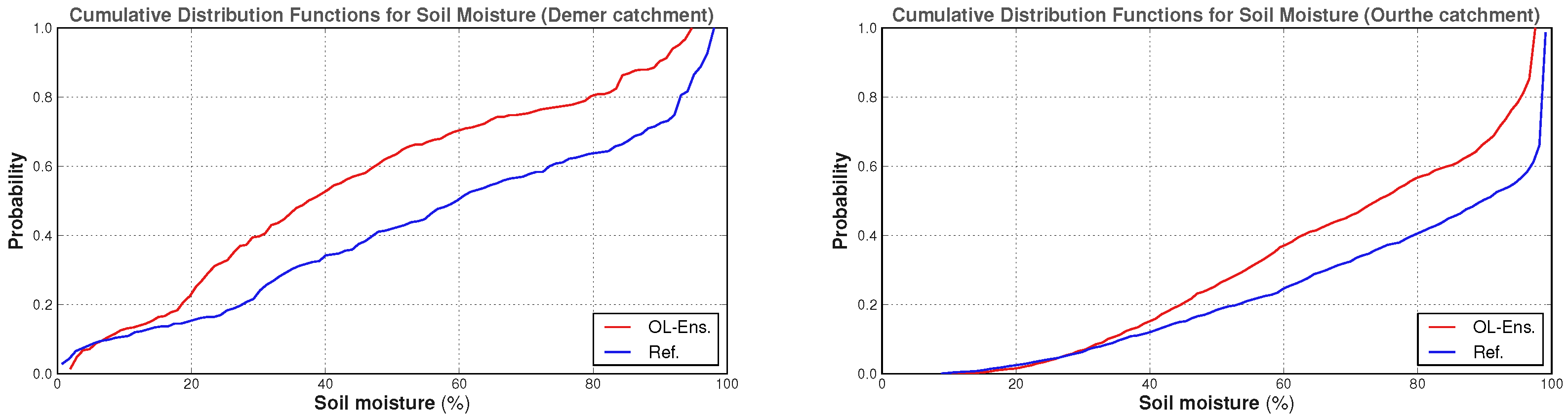
The introduction of SSM bias via ensemble perturbation is a known problem and can be solved by recentering the ensemble around a reference deterministic simulation as in, e.g., [49]. This approach assumes that the ensemble spread is created by adding Gaussian noise only to the model state variables in an ideal case, which is not true here, thus leading us to opt for an alternative solution for perturbation bias correction, which is as follows. We performed OL and reference simulations for the period 2010–2015 for both catchments. We then took spatial averages over the catchments to obtain the reference and the OL ensemble SSM time series. Based on the OL ensemble average and the reference time series, we constructed the cumulative distribution functions (CDFs) for SSM shown in Figure 5.
The CDFs can be used to measure the difference between the OL average and the reference soil moisture values at an equal probability. This leads to the soil moisture bias estimates (red lines) displayed in Figure 6, to which, we fitted a polynomial in order to allow for the calculation of a bias correction for any SSM value. In this case, the polynomial was of degree four for both catchments (blue lines in Figure 6).
The distributions and the bias functions in Figure 5 and Figure 6 provide the statistical properties of time series obtained after the averaging of simulated data over the catchments. The objective here was to apply a bias correction to the forecasted SCHEME model state (SSM) at each model time step, with the goal of minimizing the effect of the bias on the ensemble OL (bias as, e.g., in Figure 4) and DA performance. More specifically for the DA case, the bias-corrected SSM forecast should also enter as an input in the WCM and the Kalman equation. However, using the bias estimates of Figure 6 to correct SSM forecasts at each time step (with feedback into the model) would produce large correction values in the intermediate SSM range (e.g., between 40 % and 60 % for the Demer or 60 % and 80 % for the Ourthe in Figure 6). This would quickly lead to water accumulation in the upper soil layer under low evaporation conditions, which prevail in autumn and winter in Belgium. Therefore, the bias correction was adapted as follows to take into account the evaporation effect.
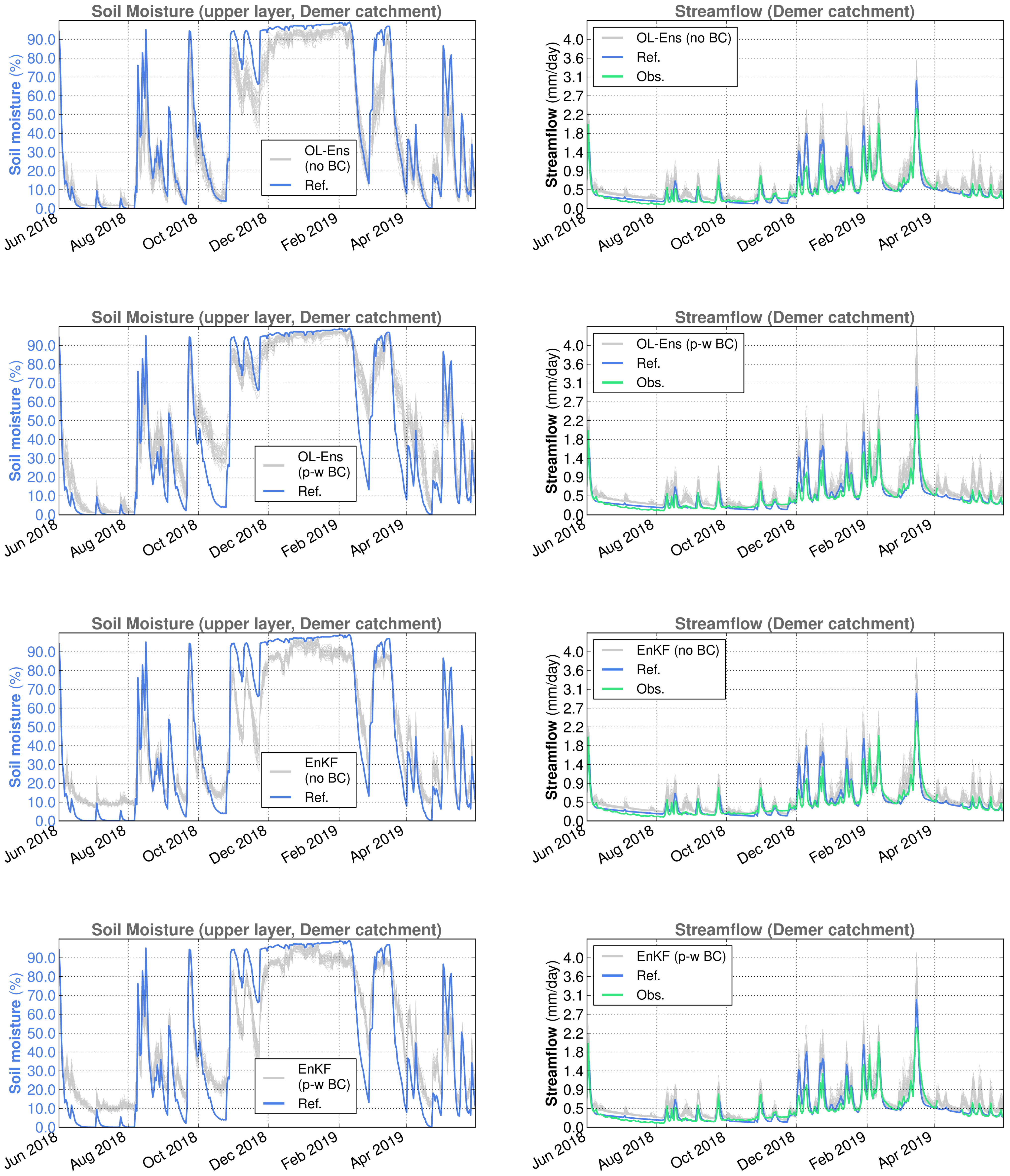
We only applied a fraction of the bias correction term above, according to the potential evapotranspiration (PET) levels. In this approach, there were two bias sub-functions defined for different intervals of PET, hence the name piece-wise bias correction (or “p-w BC” for short). More precisely, if B is the SSM bias provided by the bias function (Figure 6) and SSM bc is the bias-corrected surface soil moisture, then
SSM bc = SSM C 1 · B , if PET < P 0 SSM C 2 · B , if PET P 0 .
The PET threshold is P 0 = 1.0 mm / day for Demer and P 0 = 0.8 mm / day for Ourthe. The constants C 1 and C 2 adjusting the bias correction were calculated by minimizing the OL SSM bias relative to a deterministic simulation over the period 2010–2015. The values were C 1 = 0.20 , C 2 = 0.60 for the Demer, and C 1 = 0.08 , C 2 = 0.25 for the Ourthe (resulting in a bias of 1.93 % for the Demer and 2.26 % for the Ourthe catchment). In short, the correction given by Equation (12) was applied to the forecasted SSM at each model time step for either the OL or DA simulation, and it ensured that a bias-corrected SSM enters as an input in the WCM and the Kalman equation.

3. Results

Three different types of experiments were performed with the SCHEME model: the reference or deterministic run, the open loop (OL) and the data assimilation (DA) runs, depicted in Figure 7. The OL and DA experiments produce ensembles of simulated data and can be with or without the bias correction of Section 2.3.3 (not shown in the figure for simplicity).
The results of the reference, OL and DA experiments with the SCHEME model are given in Figure 8 and Figure 9 for the Demer catchment and in Figure 10 and Figure 11 for the Ourthe catchment. These figures illustrate all of the possible simulation options, namely OL and the EnKF with and without the application of the piece-wise bias correction (cf. Section 2.3.3). For brevity, only two years are presented here, June 2016–May 2017 and June 2018–May 2019, out of five years of the study period.
The surface soil moisture (SSM) time series have significant differences between the Demer and the Ourthe catchments. In the Ourthe, the period of time with SSM values near the saturation is considerably longer than in the Demer. In addition, SSM never reaches values close to zero in the Ourthe, whereas this happens every year in the Demer. Short-time-scale SSM variations are determined by rainfall and the season of the year. The alternation of wet and dry periods in summer, low elevation and limited forest presence are at the origin of the great SSM variability in the Demer catchment.
A visual inspection of Figure 8, Figure 9, Figure 10 and Figure 11 suggests that the OL SSM ensembles without bias correction are negatively biased relative to the reference simulation, in line with Section 2.3.3.
The effect of backscatter DA is evident at the level of soil moisture, with varying features depending on the catchment. For example, in the case of the Demer catchment, under dry conditions, DA yields higher SSM values when combined with piece-wise SSM bias correction than both the reference simulation and DA without bias correction (cf. Figure 8 and Figure 9). This leads to slightly higher streamflow values under bias correction and dry conditions. On the other hand, the application of SSM bias correction does not seem to have a substantial impact in the Ourthe catchment when DA takes place (cf. Figure 10 and Figure 11).
The streamflow ensembles generally appear to be positively biased relative to observations and the reference simulation. The differences between the simulated (reference, OL and EnKF average) and observed streamflow time series are quantified using well-established statistical scores such as bias (B), root mean square error (RMSE), Pearson correlation coefficient (R) and Nash–Sutcliffe efficiency coefficient (NSE). Such scores are calculated annually and for the whole five-year period from June 2014 to May 2019. Although the streamflow output of the SCHEME model is sensitive to SSM fluctuations over short time periods as well, multiannual metrics reflect the combined effect of a variety of hydrological conditions and better represent the SSM bias correction effect. The results of such statistical scores for all possible combinations of data and time periods are shown in Table 4 and Table 5, with multi-year summary statistics at the bottom.
The statistics show that the OL experiments introduce positive streamflow biases in all cases without exception. Indeed, the bias of each OL streamflow simulation is larger than the bias of the corresponding reference simulation. In terms of the NSE, the performance of the OL streamflow ensembles obtained is generally lower than the performance of the corresponding reference simulations, with some exceptions (first two years in Table 4, second and third year in Table 5). This is mainly due to the application of precipitation perturbations during the OL runs.
One can consider the ensemble pairs OL–EnKF under the same conditions, i.e., both without bias correction or both with piece-wise bias correction. According to the scores in the tables, the performance difference in terms of RMSE or NSE between the OL and EnKF is larger when both are generated by the application of the SSM piece-wise bias correction during the corresponding model runs.
Although there is not a clear conclusion from the statistical scores over long time periods, there are several cases in both catchments where an improvement (decreased errors or increased NSE) in streamflow estimations is observed in the DA experiments. In other instances, the reference simulation has a better performance than the EnKF ensemble average. The most characteristic case is the year June 2018–May 2019 in the Demer catchment, where DA leads to a significant decrease in NSE. The very opposite is the year June 2016–May 2017 in the Ourthe catchment, characterized by a large improvement in the simulation performance after DA.

4. Discussion

4.1. DA Performance

The streamflow results obtained in this study reveal several aspects of backscatter DA in a hydrological model. The impact is not systematically positive: it differs between the two catchments and through time, with the succession of periods of positive and negative or negligible effect. Over the full 5-year period, and in terms of the NSE, DA leads to a little improvement over the reference streamflow simulation in the Ourthe catchment and to a little deterioration in the Demer catchment, regardless of whether the bias correction is implemented or not.
At the yearly time scale, the period June 2018–May 2019 is remarkable for the Demer catchment because it is characterized by a performance deterioration of the DA (cf. Table 4), particularly when the bias correction is applied. We argue that this is due to unsuitable soil moisture levels after the DA update. Indeed, as we can see in Figure 9, backscatter DA increases the SSM compared to the reference experiment during two months in summer 2018 and two months in spring 2019. As a result, the precipitation in these months yields an increased streamflow.
Figure 12 explains why DA-updated SSM appears to be increased in June and July 2018 with respect to the deterministic run, even without the bias correction. We observe that the innovation (here, the difference between ASCAT and WCM backscatter) is, for the most part, positive in these months, and, when it is negative, the soil moisture to which it has to be applied is nearly zero. This will trigger the random generation of SSM according to the tolerance introduced in Equation (10), often resulting in increased SSM values.
The SSM update through DA can have a different effect in other cases, as we see in Table 5 for the Ourthe catchment and, in particular, in the year June 2016–May 2017. In this case, we observe a large improvement in the hydrological performance in terms of NSE. Figure 10 shows the clear association between the decreased EnKF SSM ensemble levels and the simulated EnKF streamflow ensemble, which appears to be also decreased with respect to the reference simulation. For this particular situation, we note that the SSM profile follows the ASCAT signal variations seen in Figure 13, with the exception of the second half of January 2017, which is under freezing conditions, implying that DA does not take place.
We can have varying results at shorter time scales. For example, during March 2017, we obtained, in the Demer catchment, NSE values equal to 0.833, 0.886 and 0.902 for the reference simulation and the EnKF without and with bias correction, respectively. In this case, although the SCHEME model already performs very well, backscatter DA further improves its performance (even more so with bias correction). In other instances, DA leads to large improvements in the streamflow simulations. This is the case in November and October 2017, with very large increases in model performance in terms of the NSE coefficient: 0.442 and −1.500, respectively, for the reference SCHEME model simulation, compared to 0.819 and 0.603, respectively, for the EnKF average.

4.2. Comparison with SSM Retrieval DA

Our results can be juxtaposed with analogous results obtained in [13], whereby the H-SAF H07 SSM retrieval product was assimilated into the hydrological model SCHEME in the period June 2014–May 2016 using the EnKF. The main difference is that [13] only applied a climatological bias correction depending on the grid cell and time step, and otherwise directly updated SSM in SCHEME using SSM satellite retrievals instead of backscatter. Table 6 below summarizes the statistical scores for the assimilation of the H-SAF SSM retrieval product and the C-band backscatter signals over the common time period. The comparison was performed for the backscatter EnKF experiment without perturbation bias correction for SSM since, in [13], SSM is used without perturbation bias correction as well.
In the year June 2014–May 2015, the H07 DA presents higher errors when compared to the reference simulation, which leads to a clearly lower NSE value. The bias of the backscatter DA is consistently lower than both the reference and the H07 EnKF mean in all cases. Overall, for the two-year period considered here, the backscatter DA is characterized by lower errors and a higher NSE coefficient, underlining the potential of the method for hydrological applications.

4.3. Remaining Bias Issues

Another factor to consider here is the nonlinear character of the SCHEME model and its piece-wise continuity, given that the SSM value at each grid cell is directly related to the generation of streamflow through a threshold exceedance. More precisely, if, during a precipitation event, SSM exceeds its upper limit, then the surplus is used by the model to compute contributions to the streamflow and infiltration to the lower soil layer. In the EnKF, precipitation is perturbed. A precipitation value that is not able to produce streamflow can reach, after the application of perturbations, higher values that are able to fill the upper soil layer and exceed its capacity, leading to streamflow generation. Therefore, the EnKF itself, by its own very nature, combined with the model non-linearity, introduces bias at the level of streamflow in particular. In [13], a simple method used to address this issue has been proposed. Due to the highly non-linear observation operator, the same method cannot be applied in the present case, and developing an alternative is beyond the scope of this study.

5. Conclusions

This study presents the first ASCAT backscatter data assimilation (DA) system associated with the operational model SCHEME of the Royal Meteorological Institute of Belgium. The data assimilation system shows a varying performance in terms of streamflow statistics depending on the catchment, the time scale and the hydrological conditions. Over the available 5-year period, an improvement in the DA streamflow performance over a deterministic simulation is observed only in the Ourthe catchment. The hydrological conditions play an important role as well. In our EnKF implementation, very dry conditions degrade the performance of the DA streamflow ensembles because the corresponding SSM ensembles after the DA update never drop as low as the reference SSM SCHEME model run.
The main limitation of our system is in the generation of ensembles and in addressing SSM biases associated with it. While the perturbation bias correction attempts to minimize the SSM bias between a deterministic and ensemble simulation, it does not necessarily improve the performance of the ensemble streamflow simulations with respect to the observations. This suggests that the proposed bias correction method might not be optimal or not blend well with our DA implementation. Other biases (cf. Section 4.3) certainly play a role here. Future research should thus attempt to optimize the bias correction scheme.
Nevertheless, the negative effects of the ensemble perturbations do not limit the assessment of the DA impact relative to the OL performance. The comparison between the DA and the OL simulations gives insight into the potential value of assimilating backscatter observations into the SCHEME model. The DA improves streamflow over the OL simulations, whereas the DA improvement over the deterministic reference simulation is not clear. Furthermore, the DA improvement over the OL is systematically visible over the full time series in the Ourthe catchment. This study also demonstrated the advantage of using backscatter DA over SSM retrieval DA for the performance of streamflow simulations. These results further support the idea of pursuing backscatter DA, even for catchments with a higher vegetation density, such as the Ourthe catchment.
Finally, new perspectives for hydrological forecasting can be foreseen. We have shown that the updated SSM after DA can be considerably different from the reference simulation. Therefore, it would be very interesting to use updated SSM to generate new initial conditions for hydrological forecasts. The study of this forecasting setup can be combined with the optimization attempts mentioned previously to provide more insight toward the potential of backscatter DA in hydrology.

Author Contributions

Conceptualization, P.B., E.R., S.V. and G.D.L.; methodology, P.B., A.C. and G.D.L.; software, P.B., S.M. and H.L.; formal analysis, P.B.; investigation, P.B.; writing—original draft preparation, P.B.; writing—review and editing, P.B., A.C., E.R., S.V., S.M., H.L., M.B. and G.D.L.; visualization, P.B.; supervision, S.V.; funding acquisition, E.R. and S.V. All authors have read and agreed to the published version of the manuscript.

Funding

This research was funded by the Belgian Science Policy Office (BELSPO) through the STEREO III project EODAHR (Improving early warnings through Earth observation data assimilation and hydrological retrospective forecast, contract no. SR/00/376, 2019–2021).

Institutional Review Board Statement

Not applicable.

Informed Consent Statement

Not applicable.

Data Availability Statement

ASCAT data are available through the EUMETSAT Earth Observation Portal (https://eoportal.eumetsat.int (accessed on 1 September 2022)) and LAI data through the Copernicus Global Land Service (https://land.copernicus.eu/global/products/lai (accessed on 1 September 2022)). SCHEME model output data can be provided upon request.

Acknowledgments

The authors would like to thank Sebastian Hahn (TU Wien, Vienna, Austria) for clarifying several points of the TU Wien change detection method.

Conflicts of Interest

The authors declare no conflict of interest.

Abbreviations

The following abbreviations are used in this manuscript:
ASCATAdvanced scatterometer
CGLSCopernicus Global Land Service
ECMWFEuropean Centre for Medium-Range Weather Forecasts
EnKFEnsemble Kalman filter
EUMETSATEuropean Organisation for the Exploitation of Meteorological Satellites
FCField capacity
LAILeaf area index
MetOpMeteorological Operational Satellite
NSENash–Sutcliffe efficiency coefficient
OLOpen loop (simulation)
PETPotential evapotranspiration
PROBA-VProject for On-Board Autonomy–Vegetation
PWPPermanent wilting point
RMIRoyal Meteorological Institute of Belgium
RMSERoot mean square error
SCE-UAShuffled complex evolution algorithm - University of Arizona
SCHEMESCHEldt and MEuse (hydrological model)
SSMSurface soil moisture
SSM v Surface soil moisture (volumetric)
WCMWater cloud model

References

  1. Crow, W.T.; Chen, F.; Reichle, R.H.; Xia, Y.; Liu, Q. Exploiting soil moisture, precipitation, and streamflow observations to evaluate soil moisture/runoff coupling in land surface models. Geophys. Res. Lett. 2018, 45, 4869–4878. [Google Scholar] [CrossRef]
  2. Ermida, S.L.; Trigo, I.F.; DaCamara, C.C.; Jiménez, C.; Prigent, C. Quantifying the clear-sky bias of satellite land surface temperature using microwave-based estimates. J. Geophys. Res. Atmos. 2019, 124, 844–857. [Google Scholar] [CrossRef]
  3. Li, Z.; Stoffelen, A.; Verhoef, A.; Verspeek, J. Numerical weather prediction Ocean Calibration for the Chinese-French Oceanography Satellite wind scatterometer and wind retrieval evaluation. Earth Space Sci. 2021, 8, e2020EA001606. [Google Scholar] [CrossRef]
  4. Stoffelen, A.; Verspeek, J.A.; Vogelzang, J.; Verhoef, A. The CMOD7 geophysical model function for ASCAT and ERS wind retrievals. IEEE J. Sel. Topics Appl. Earth Obs. Remote Sens. 2017, 10, 2123–2134. [Google Scholar] [CrossRef]
  5. Belmonte Rivas, M.; Verspeek, J.; Verhoef, A.; Stoffelen, A. Bayesian Sea Ice Detection with the Advanced Scatterometer ASCAT. IEEE Trans. Geosci. Remote Sens. 2012, 50, 2649–2657. [Google Scholar] [CrossRef]
  6. Belmonte Rivas, M.; Otosaka, I.; Stoffelen, A.; Verhoef, A. A scatterometer record of sea ice extents and backscatter: 1992–2016. Cryosphere 2018, 12, 2941–2953. [Google Scholar] [CrossRef] [Green Version]
  7. Wagner, W.; Hahn, S.; Kidd, R.; Melzer, T.; Bartalis, Z.; Hasenauer, S.; Figa-Saldaña, J.; de Rosnay, P.; Jann, A.; Schneider, S.; et al. The ASCAT soil moisture product: A review of its specifications, validation results, and emerging applications. Meteorol. Z. 2013, 22, 5–33. [Google Scholar] [CrossRef] [Green Version]
  8. Tong, R.; Parajka, J.; Salentinig, A.; Pfeil, I.; Komma, J.; Széles, B.; Kubàn, M.; Valent, P.; Vreugdenhil, M.; Wagner, W.; et al. The value of ASCAT soil moisture and MODIS snow cover data for calibrating a conceptual hydrologic model. Hydrol. Earth Syst. Sci. 2021, 25, 1389–1410. [Google Scholar]
  9. Vreugdenhil, M.; Hahn, S.; Melzer, T.; Bauer-Marschallinger, B.; Reimer, C.; Dorigo, W.A.; Wagner, W. Assessing vegetation dynamics over mainland Australia with Metop ASCAT. IEEE J. Sel. Top. Appl. Earth Obs. Remote Sens. 2017, 10, 2240–2248. [Google Scholar] [CrossRef]
  10. Pauwels, V.R.N.; Hoeben, R.; Verhoest, N.E.C.; De Troch, F.P.; Troch, P.A. Improvement of TOPLATS-based discharge predictions through assimilation of ERS-based remotely sensed soil moisture values. Hydrol. Process. 2002, 16, 995–1013. [Google Scholar] [CrossRef]
  11. Massari, C.; Brocca, L.; Tarpanelli, A.; Moramarco, T. Data Assimilation of Satellite Soil Moisture into Rainfall-Runoff Modelling: A Complex Recipe? Remote Sens. 2015, 7, 11403–11433. [Google Scholar] [CrossRef]
  12. Wanders, N.; Karssenberg, D.; de Roo, A.; de Jong, S.M.; Bierkens, M.F.P. The suitability of remotely sensed soil moisture for improving operational flood forecasting. Hydrol. Earth Syst. Sci. 2014, 18, 2343–2357. [Google Scholar] [CrossRef] [Green Version]
  13. Baguis, P.; Roulin, E. Soil Moisture Data Assimilation in a Hydrological Model: A Case Study in Belgium Using Large-Scale Satellite Data. Remote Sens. 2017, 10, 820. [Google Scholar] [CrossRef] [Green Version]
  14. Seo, E.; Lee, M.I.; Reichle, R.H. Assimilation of SMAP and ASCAT soil moisture retrievals into the JULES land surface model using the Local Ensemble Transform Kalman Filter. Remote Sens. Environ. 2021, 253, 112222. [Google Scholar] [CrossRef]
  15. Albergel, C.; Munier, S.; Leroux, D.J.; Dewaele, H.; Fairbairn, D.; Barbu, A.L.; Gelati, E.; Dorigo, W.; Faroux, S.; Meurey, C.; et al. Sequential assimilation of satellite-derived vegetation and soil moisture products using SURFEX v8.0: LDAS-Monde assessment over the Euro-Mediterranean area. Geosci. Model. Dev. 2017, 10, 3889–3912. [Google Scholar] [CrossRef] [Green Version]
  16. Kumar, S.V.; Mocko, D.M.; Wang, S.; Peters-Lidard, C.D.; Borak, J. Assimilation of Remotely Sensed Leaf Area Index into the Noah-MP Land Surface Model: Impacts on Water and Carbon Fluxes and States over the Continental United States. J. Hydrometeorol. 2019, 20, 1359–1377. [Google Scholar] [CrossRef]
  17. De Lannoy, G.J.M.; Reichle, R.H. Global assimilation of multiangle and multipolarization SMOS brightness temperature observations into the GEOS-5 Catchment Land Surface Model for soil moisture estimation. J. Hydrometeorol. 2016, 17, 669–691. [Google Scholar] [CrossRef] [Green Version]
  18. De Lannoy, G.J.M.; Bechtold, M.; Albergel, C.; Brocca, L.; Calvet, J.-C.; Carrassi, A. Perspective on satellite-based land data assimilation to estimate water cycle components in an era of advanced data availability and model sophistication. Front. Water 2022, 4, 981745. [Google Scholar] [CrossRef]
  19. Evensen, G.; Vossepoel, F.C.; van Leeuwen, P.J. Data Assimilation Fundamentals; Springer Nature: Cham, Switzerland, 2022. [Google Scholar]
  20. Reichle, R.H.; McLaughlin, D.B.; Entekhabi, D. Hydrologic Data Assimilation with the Ensemble Kalman Filter. Mon. Weather Rev. 2002, 130, 103–114. [Google Scholar] [CrossRef]
  21. Kalman, R.E. A new approach to linear filtering and prediction problems. J. Basic Eng. 1960, 82, 35–45. [Google Scholar] [CrossRef] [Green Version]
  22. De Lannoy, G.J.M.; Houser, P.R.; Pauwels, V.R.N.; Verhoest, N.E.C. Assessment of model uncertainty for soil moisture through ensemble verification. J. Geophys. Res. 2006, 111, 1–18. [Google Scholar]
  23. Li, H.; Luo, L.; Wood, E.F.; Schaake, J. The role of initial conditions and forcing uncertainties in seasonal hydrologic forecasting. J. Geophys. Res. 2009, 114, D04114. [Google Scholar] [CrossRef]
  24. DeChant, C.M.; Moradkhani, H. Improving the characterization of initial condition for ensemble streamflow prediction using data assimilation. Hydrol. Earth Syst. Sci. 2011, 15, 3399–3410. [Google Scholar] [CrossRef] [Green Version]
  25. Arsenault, K.; Shukla, S.; Hazra, A.; Getirana, A.; McNally, A.; Kumar, S.V.; Koster, R.D.; Peters-Lidard, C.D.; Zaitchik, B.F.; Badr, H.; et al. The NASA Hydrological Forecast System for Food and Water Security Applications. Bull. Am. Meteorol. Soc. 2020, 101, E1007–E1025. [Google Scholar] [CrossRef] [Green Version]
  26. Roulin, E.; Vannitsem, S. Skill of medium-range hydrological ensemble predictions. J. Hydrometeorol. 2005, 6, 729–744. [Google Scholar] [CrossRef]
  27. Gelsthorpe, R.V.; Schied, E.; Wilson, J.J.W. ASCAT—MetOp’s Advanced Scatterometer. ESA Bull. 2000, 102, 19–27. [Google Scholar]
  28. Attema, E.; Ulaby, F. Vegetation modeled as a water cloud. Radio Sci. 1978, 13, 357–364. [Google Scholar] [CrossRef]
  29. Shamambo, D.C.; Bonan, B.; Calvet, J.-C.; Albergel, C.; Hahn, S. Interpretation of ASCAT Radar Scatterometer Observations over Land: A Case Study over Southwestern France. Remote Sens. 2019, 11, 2842. [Google Scholar] [CrossRef] [Green Version]
  30. Lievens, H.; Martens, B.; Verhoest, N.E.C.; Hahn, S.; Reichle, R.H.; Miralles, D.G. Assimilation of global radar backscatter and radiometer brightness temperature observations to improve soil moisture on land evaporation estimates. Remote Sens. Environ. 2017, 189, 194–210. [Google Scholar]
  31. Hahn, S.; Reimer, C.; Vreugdenhil, M.; Melzer, T.; Wagner, W. Dynamic Characterization of the Incidence Angle Dependence of Backscatter Using MetOp ASCAT. IEEE J. Sel. Top. Appl. Earth Obs. Remote Sens. 2017, 10, 2348–2359. [Google Scholar] [CrossRef]
  32. Francois, M.; Santandrea, S.; Mellab, K.; Vrancken, D.; Versluys, J. The PROBA-V mission: The space segment. Int. J. Remote Sens. 2014, 35, 2548–2564. [Google Scholar] [CrossRef]
  33. Danielson, J.J.; Gesch, D.B. Global Multi-Resolution Terrain Elevation Data 2010 (GMTED2010); US Geological Survey: Washington, DC, USA, 2011; Volume 2011-1073, 23p. [CrossRef] [Green Version]
  34. Balsamo, G.; Viterbo, P.; Beljaars, A.; van den Hurk, B.; Hirschi, M.; Betts, A.K.; Scipal, K. A Revised Hydrology for the ECMWF Model: Verification from Field Site to Terrestrial Water Storage and Impact in the Integrated Forecast System. J. Hydrometeorol. 2009, 10, 623–643. [Google Scholar] [CrossRef] [Green Version]
  35. Wagner, W.; Lemoine, G.; Rott, H. A method for estimating soil moisture from ERS scatterometer and soil data. Remote Sens. Environ. 1999, 70, 191–207. [Google Scholar]
  36. Bartalis, Z.; Scipal, K.; Wagner, W. Azimuthal anisotropy of scatterometer measurements over land. IEEE Trans. Geosci. Remote Sens. 2006, 44, 2083–2092. [Google Scholar] [CrossRef]
  37. Greimeister-Pfeil, I.; Wagner, W.; Quast, R.; Hahn, S.; Steele-Dunne, S.; Vreugdenhil, M. Analysis of short-term soil moisture effects on the ASCAT backscatter-incidence angle dependence. Sci. Remote Sens. 2022, 5, 100053. [Google Scholar] [CrossRef]
  38. Sterckx, S.; Benhadj, I.; Duhoux, G.; Livens, S.; Dierckx, W.; Goor, E.; Adriaensen, S.; Heyns, W.; Van Hoof, K.; Strackx, G.; et al. The PROBA-V mission: Image processing and calibration. Int. J. Remote Sens. 2014, 35, 2565–2588. [Google Scholar] [CrossRef]
  39. Dierckx, W.; Sterckx, S.; Benhadj, I.; Livens, S.; Duhoux, G.; Van Achteren, T.; Francois, M.; Mellab, K.; Saint, G. PROBA-V mission for global vegetation monitoring: Standard products and image quality. Int. J. Remote Sens. 2014, 35, 2589–2614. [Google Scholar]
  40. Bultot, F.; Dupriez, G. Conceptual hydrological model for an average-sized catchment area. J. Hydrol. 1976, 29, 251–292. [Google Scholar] [CrossRef]
  41. Bultot, F.; Gellens, D.; Spreafico, M.; Schädler, B. Repercussions of a CO2 doubling on the waterbalance—A case study in Switzerland. J. Hydrol. 1992, 137, 199–208. [Google Scholar] [CrossRef]
  42. Bultot, F.; Dupriez, G.L.; Gellens, D. Estimated annual regime of energy-balance components, evapotranspiration and soil moisture for a drainage basin in the case of a CO2 doubling. Clim. Chang. 1988, 12, 39–56. [Google Scholar]
  43. Van den Bergh, J.; Roulin, E. Postprocessing of Medium Range Hydrological Ensemble Forecasts Making Use of Reforecasts. Hydrology 2016, 3, 21. [Google Scholar] [CrossRef] [Green Version]
  44. Penman, H. Natural evaporation from open water, bare soil and grass. Proc. Roy. Soc. Ser. A 1948, 193, 120–145. [Google Scholar]
  45. Duan, Q.Y.; Sorooshian, S.; Gupta, V.K. Optimal use of the SCE-UA global optimization method for calibrating watershed models. J. Hydrol. 1994, 158, 265–284. [Google Scholar] [CrossRef]
  46. Evensen, G. Sequential data assimilation with a nonlinear quasi-geostrophic model using Monte Carlo methods to forecast error statistics. J. Geophys. Res. Oceans 1994, 99, 10143–10162. [Google Scholar]
  47. Evensen, G. The Ensemble Kalman Filter: Theoretical formulation and practical implementation. Ocean Dyn. 2003, 53, 343–367. [Google Scholar] [CrossRef]
  48. Carrassi, A.; Bocquet, M.; Bertino, L.; Evensen, G. Data assimilation in the geosciences: An overview of methods, issues, and perspectives. Wiley Interdiscip. Rev. Clim. Chang. 2018, 9, e535. [Google Scholar] [CrossRef] [Green Version]
  49. Ryu, D.; Crow, W.T.; Zhan, X.; Jackson, T.J. Correcting Unintended Perturbation Biases in Hydrologic Data Assimilation. J. Hydrometeorol. 2009, 10, 734–750. [Google Scholar] [CrossRef]
Figure 1. Left: the river basins (Scheldt and Meuse, in light colors) and the catchments (Demer and Ourthe, in dark colors) included in the present study. Right: the Demer and Ourthe catchments with topographic features and their outlets. The elevation data are based on [33].
Remotesensing 14 05740 g001
Figure 2. Soil types following [34].
Remotesensing 14 05740 g002
Figure 3. Diagram of processes of the SCHEME model. Model parameters: (1) w d s x , threshold value for upper soil reservoir; (2) scr ( 4 ) , seasonal runoff coefficients; (3) μ , redirection coefficient for surface flow; (4) a, b and c, parameters describing a unit hydrograph; (5) α 1 and α 2 , recession coefficients of the underground reservoirs; (6) v and D, routing module parameters.
Remotesensing 14 05740 g003
Figure 4. Spatially averaged SSM over the Demer and the Ourthe catchments. The reference simulation obtained with the deterministic SCHEME model run and the original open loop ensembles (OL-Ens) are depicted (June 2011–May 2012).
Remotesensing 14 05740 g004
Figure 5. Cumulative distribution functions for surface soil moisture based on spatially averaged open loop and reference data for the period 2010–2015.
Remotesensing 14 05740 g005
Figure 6. Bias functions for SSM based on the CDFs for the period 2010–2015 (original data and curve fit).
Remotesensing 14 05740 g006
Figure 7. The three types of experiments performed with the SCHEME model.
Remotesensing 14 05740 g007
Figure 8. Spatially averaged surface soil moisture (reference simulation and ensemble members) and streamflow (reference simulation, observations and ensemble members) for the Demer catchment in SCHEME model simulations, June 2016–May 2017. From top to bottom: OL without bias correction, OL with piece-wise bias correction, EnKF without bias correction, EnKF with piece-wise bias correction.
Remotesensing 14 05740 g008
Figure 9. Spatially averaged surface soil moisture (reference simulation and ensemble members) and streamflow (reference simulation, observations and ensemble members) for the Demer catchment in SCHEME model simulations, June 2018–May 2019. From top to bottom: OL without bias correction, OL with piece-wise bias correction, EnKF without bias correction, EnKF with piece-wise bias correction.
Remotesensing 14 05740 g009
Figure 10. Spatially averaged surface soil moisture (reference simulation and ensemble members) and streamflow (reference simulation, observations and ensemble members) for the Ourthe catchment in SCHEME model simulations, June 2016–May 2017. From top to bottom: OL without bias correction, OL with piece-wise bias correction, EnKF without bias correction, EnKF with piece-wise bias correction.
Remotesensing 14 05740 g010
Figure 11. Spatially averaged surface soil moisture (reference simulation and ensemble members) and streamflow (reference simulation, observations and ensemble members) for the Ourthe catchment in SCHEME model simulations, June 2018–May 2019. From top to bottom: OL without bias correction, OL with piece-wise bias correction, EnKF without bias correction, EnKF with piece-wise bias correction.
Remotesensing 14 05740 g011
Figure 12. Spatially averaged backscatter, simulated (WCM) and observed (ASCAT) and SSM (deterministic SCHEME run) for the Demer catchment, June 2018–May 2019.
Remotesensing 14 05740 g012
Figure 13. Spatially averaged backscatter, simulated (WCM) and observed (ASCAT) and SSM (deterministic SCHEME run) for the Ourthe catchment, June 2016–May 2017.
Remotesensing 14 05740 g013
Table 1. Synoptic streamflow climatology.
Streamflow (mm/Day)ClimatologicalStudy Period
1971–20002010–2019
Demer catchment
Average0.620.61
Record low0.020.10
Minimum monthly average0.380.35
Record high2.922.74
Maximum monthly average0.891.07
Ourthe catchment
Average1.201.12
Record low0.030.06
Minimum monthly average0.320.32
Record high19.7914.74
Maximum monthly average2.232.78
Table 2. Synoptic precipitation climatology (totals, areal averaged).
Precipitation (mm)ClimatologicalStudy Period
1966–19952010–2019
Demer catchment
Yearly average768726
Record high in one day5650
Minimum monthly average5036
Maximum monthly average7782
Ourthe catchment
Yearly average988930
Record high in one day7744
Minimum monthly average6945
Maximum monthly average100121
Table 3. Synoptic temperature climatology (areal averaged).
Temperature ( ° C)ClimatologicalStudy Period
1966–19952010–2019
Demer catchment
Average9.810.8
Record low−19.5−15.6
Minimum monthly average2.83.2
Record high35.640.0
Maximum monthly average17.719.1
Ourthe catchment
Average8.39.0
Record low−19.0−15.5
Minimum monthly average0.91.14
Record high34.036.9
Maximum monthly average16.517.4
Table 4. Synoptic statistics for streamflow, Demer catchment. The unit for bias and RMSE is mm/day and the scores are calculated with respect to the streamflow observations.
BRMSERNSE
1 June 2014–31 May 2015
Reference simulation−0.090.200.930.80
OL mean, no BC0.060.200.930.81
OL mean, p-w BC0.120.240.930.73
EnKF mean, no BC0.030.190.920.82
EnKF mean, p-w BC0.070.210.920.79
1 June 2015–31 May 2016
Reference simulation−0.110.200.940.84
OL mean, no BC0.060.170.950.88
OL mean, p-w BC0.130.220.950.81
EnKF mean, no BC0.040.170.950.89
EnKF mean, p-w BC0.070.190.940.87
1 June 2016–31 May 2017
Reference simulation−0.060.250.920.82
OL mean, no BC0.050.250.920.82
OL mean, p-w BC0.120.290.920.75
EnKF mean, no BC−0.000.250.910.83
EnKF mean, p-w BC0.030.250.910.82
1 June 2017–31 May 2018
Reference simulation−0.060.160.950.84
OL mean, no BC0.110.190.950.75
OL mean, p-w BC0.150.230.960.65
EnKF mean, no BC0.090.170.950.80
EnKF mean, p-w BC0.110.190.950.75
1 June 2018–31 May 2019
Reference simulation0.040.170.910.77
OL mean, no BC0.150.230.920.61
OL mean, p-w BC0.190.260.940.51
EnKF mean, no BC0.150.220.930.64
EnKF mean, p-w BC0.160.230.930.59
1 June 2014–31 May 2019
Reference simulation−0.060.200.920.83
OL mean, no BC0.080.210.930.81
OL mean, p-w BC0.190.260.940.51
EnKF mean, no BC0.060.200.920.82
EnKF mean, p-w BC0.090.210.930.80
Table 5. Synoptic statistics for streamflow, Ourthe catchment. The unit for bias and RMSE is mm/day and the scores are calculated with respect to the streamflow observations.
BRMSERNSE
1 June 2014–31 May 2015
Reference simulation0.060.580.880.77
OL mean, no BC0.140.590.880.75
OL mean, p-w BC0.280.710.840.64
EnKF mean, no BC−0.090.610.870.74
EnKF mean, p-w BC−0.070.620.860.73
1 June 2015–31 May 2016
Reference simulation0.380.800.880.67
OL mean, no BC0.400.770.880.69
OL mean, p-w BC0.520.910.850.58
EnKF mean, no BC−0.020.580.920.82
EnKF mean, p-w BC0.010.580.920.83
1 June 2016–31 May 2017
Reference simulation0.390.730.840.43
OL mean, no BC0.430.700.850.49
OL mean, p-w BC0.550.820.840.30
EnKF mean, no BC0.110.510.860.72
EnKF mean, p-w BC0.140.510.860.72
1 June 2017–31 May 2018
Reference simulation0.030.450.950.89
OL mean, no BC0.160.560.930.83
OL mean, p-w BC0.300.650.910.78
EnKF mean, no BC−0.010.600.930.81
EnKF mean, p-w BC0.000.580.930.82
1 June 2018–31 May 2019
Reference simulation0.060.610.870.76
OL mean, no BC0.240.640.880.73
OL mean, p-w BC0.340.720.860.66
EnKF mean, no BC0.180.640.870.73
EnKF mean, p-w BC0.190.650.870.73
1 June 2014–31 May 2019
Reference simulation0.190.640.880.74
OL mean, no BC0.270.660.880.73
OL mean, p-w BC0.400.770.860.63
EnKF mean, no BC0.030.590.890.78
EnKF mean, p-w BC0.050.590.890.78
Table 6. Synoptic statistics for streamflow under H07 and backscatter data assimilation, Demer catchment. The unit for bias and RMSE is mm/day.
BRMSERNSE
1 June 2014–31 May 2015
Reference simulation−0.090.200.930.80
EnKF, backscatter DA0.030.190.920.82
EnKF, H07 DA0.100.220.920.76
1 June 2015–31 May 2016
Reference simulation−0.110.200.940.84
EnKF, backscatter DA0.040.170.950.89
EnKF, H07 DA0.070.160.960.89
1 June 2014–31 May 2016
Reference simulation−0.100.200.930.82
EnKF, backscatter DA0.040.180.930.86
EnKF, H07 DA0.090.200.940.83
Publisher’s Note: MDPI stays neutral with regard to jurisdictional claims in published maps and institutional affiliations.

