Article

Comparing Gaofen-5, Ground, and Huanjing-1A Spectra for the Monitoring of Soil Salinity with the BP Neural Network Improved by Particle Swarm Optimization

1
Key Laboratory of Desert and Desertification, Northwest Institute of Eco-Environment and Resources, Chinese Academy of Sciences, Lanzhou 730000, China
2
University of Chinese Academy of Sciences, Beijing 100049, China
3
Drylands Salinization Research Station, Northwest Institute of Eco-Environment and Resources, Chinese Academy of Sciences, Lanzhou 730000, China
*
Author to whom correspondence should be addressed.
Remote Sens. 2022, 14(22), 5719; https://doi.org/10.3390/rs14225719
Submission received: 26 October 2022 / Revised: 10 November 2022 / Accepted: 10 November 2022 / Published: 12 November 2022

Abstract

:
Most of the world’s saline soils are found in arid or semiarid areas, where salinization is becoming serious. Ground laboratory hyperspectral data (analytical spectral devices, ASD) as well as spaceborne hyperspectral data, including Gaofen-5 (GF-5) and Huanjing-1A (HJ-1A), provide convenient salinity monitoring. However, the difference among ASD, GF-5, and HJ-1A spectra in salinity monitoring remains unclear. So, we used ASD, GF-5, and HJ-1A spectra as data sources in Gaotai County of Hexi Corridor, which has been affected by salinization. For a more comprehensive comparison of the three spectra datum, four kinds of band screening methods, including Pearson correlation coefficient (PCC), principal component analysis (PCA), successive projections algorithm (SPA), and random forest (RF) were used to reduce the dimension of hyperspectral data. Particle swarm optimization (PSO) was used to improve the random initialization of weights and thresholds of the back propagation neural network (BPNN) model. The results showed that root mean square error (RMSE) and determination of the coefficients (R2) of models based on ASD and HJ-1A spectra were basically similar. ASD spectra (RMSE = 4 mS·cm−1, R2 = 0.82) and HJ-1A (RMSE = 2.98 mS·cm−1, R2 = 0.93) performed better than GF-5 spectra (RMSE = 6.45 mS·cm−1, R2 = 0.67) in some cases. The good modelling result of HJ-1A and GF-5 data confirmed that spaceborne hyperspectral imagery has great potential in salinity mapping. Then, we used HJ-1A and GF-5 hyperspectral imagery to map soil salinity. The results of GF-5 and HJ-1A showed that extremely and highly saline soil mainly occurred in grassland and the southern part of arable land in Gaotai County. Other lands mainly featured non-saline and slightly saline soil. This can provide a reference for salinity monitoring research.

1. Introduction

Soil salinization is a kind of land degradation that seriously threatens food security and sustainable social development, including primary and secondary salinization [1,2]. The excessive salt in the soil is not conducive to the growth and development of plants, reducing water absorption by roots [3]. Currently, 20% of the world’s irrigated area is affected by soil salinization and waterlogging. This proportion will continue to increase in the future [4]. Therefore, monitoring soil salinity with methods such as mathematical models is necessary.
Linear models have limitations and are only suitable for cases with linear relationships between parameters. In contrast, nonlinear machine learning models are more suitable for cases with no linear relationship between parameters [5,6,7,8]. Fathizad et al. used a random forest (RF) machine learning model to estimate soil salinity in the Yazd-Ardakan Plain of Iran, and the accuracy of the model was optimal (R2 = 0.73) [9]. At present, a large number of studies use intelligent optimization algorithms to optimize machine learning algorithms for better prediction, such as particle swarm optimization–extreme learning machine (PSO-ELM) [10], particle swarm optimization–support vector machine (PSO-SVM) [11,12], ant colony optimization–support vector machine (ACO-SVM) [13], whale optimization algorithm–extreme learning machine (WOA-ELM) [14], particle swarm optimization–Elman recurrent neural network (PSO-ERNN) [15], modified whale optimization algorithm–artificial neural network (MWOA-ANN) [16], etc. Liu et al. proved that the particle swarm optimization–back propagation neural network (PSO-BPNN) had the most minor error compared with traditional BPNN [17]. In terms of soil salinization, there are many studies using machine learning algorithms (e.g., BPNN, RF, ELM, etc.) [7,9,18], but few studies using intelligent optimization algorithms (e.g., PSO, ACO, WOA, etc.) to optimize machine learning algorithms [19].
Multispectral, hyperspectral, and microwave remote sensing on different platforms are widely used in soil organic matter, phosphorus, salinity, and potassium [20,21]. Zhang et al. and Taghadosi et al. proved that microwave remote sensing data with the advantage of working in all weather and strong penetrability is conducive to the retrieval of soil salinity [22,23]. Multispectral data with low spectral resolution and mixed pixels lacks diagnostic spectra for predicting soil information, so spatial resolution and other auxiliary information are essential for multispectral data. Ma et al. combined unmanned aerial vehicle (UAV) multispectral images characterized by high spatial resolution with large-scale Sentinel-2A data and then conducted an accurate inversion research of soil salt content for China’s Kenli district [24]. Khanna et al. found that there was a loss of the ability to detect vegetation stress with broader spectral bands [25]. Other studies have shown that fine spectral resolution of hyperspectral data was beneficial for improving estimation accuracy [26,27]. Hyperspectral data (e.g., GF-5, ZY-1-02D, PRISMA, AVIRIS, EO-1 Hyperion and HJ-1A, etc.) is increasingly widely used [28,29,30,31,32,33,34]. Hu et al. estimated field-scale soil salinity using hyperspectral cameras mounted on a drone platform and obtained an ideal result [30]. Hyperspectral data have characteristics of high spectral resolution and band connection but information redundancy. Preprocessing the hyperspectral data can improve inversion accuracy. Reducing the dimension of hyperspectral data is very important. The fractional-order differential is another conducive method to mining details [35,36,37]. Wang et al. found that the optimal inversion model for soil organic matter in China’s Aibi Lake was gray relational analysis–back propagation neural network (GRA-BPNN) with 1.2 order data source [38].
The process of salinization is mainly the accumulation of soluble salt carried by water. Gaotai County of Hexi Corridor is located in the middle reaches of the Heihe River Basin, where soil salinization is typical due to the relatively dry climate, intense evaporation, and unreasonable farming–animal husbandry irrigation. This area is located in the arid region of Northwest China. Research on soil salinization of Gaotai County is conducive to preventing land degradation and protecting fragile ecological environments in Hexi Corridor. Electrical conductivity (EC) is an important surrogate indicator of soil salinity and there is a significant correlation between EC and soil salinity [39,40,41]. Currently, due to the low cost of multispectral imagery and the difficult availability of hyperspectral datasets [42], few studies have compared the feasibility of ground and spaceborne hyperspectral data in soil salinity monitoring. In order to explore the applicability of ASD, GF-5, and HJ-1A hyperspectral data in soil salinity monitoring and large-scale soil salinity mapping, this research took Gaotai county in Hexi Corridor as the study area, and combined EC with ASD, HJ-1A, and GF-5 data to establish the PSO-BPNN model. We also used four band screening methods (PCC, PCA, SPA, and RF) to reduce the dimension of hyperspectral data. Therefore, we finally established five models (e.g., PCC-PSO-BPNN, PCA-PSO-BPNN, SPA-PSO-BPNN, RF-PSO-BPNN, and PSO-BPNN without band screening method) for each kind of spectra. The primary purpose is to provide a reference for soil salinity monitoring and management in the study area.

2. Study Area and Method
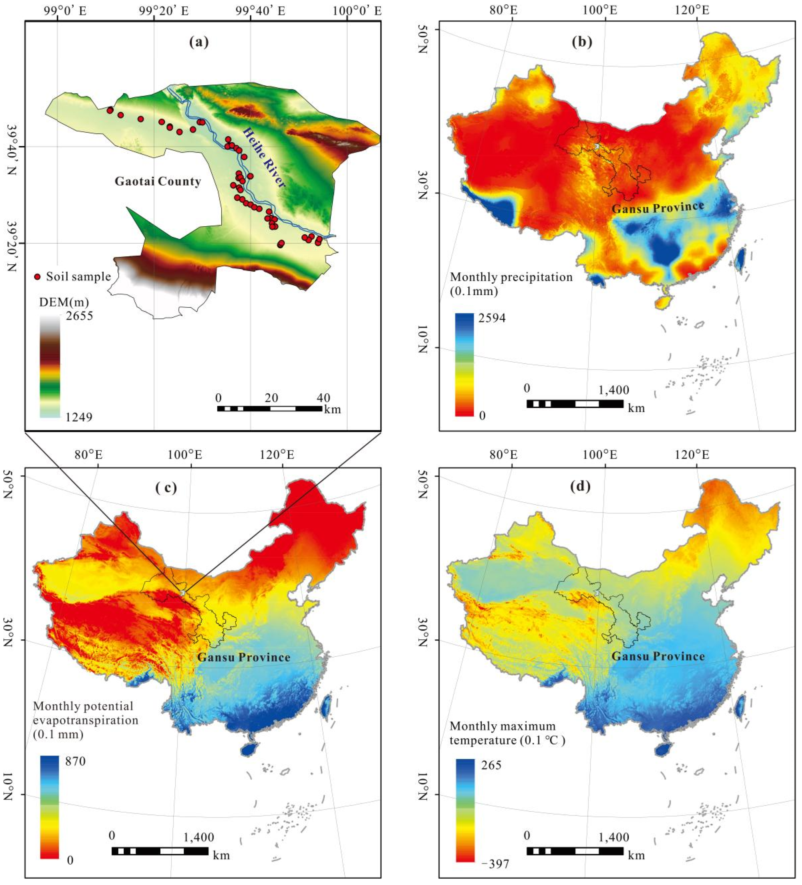
2.1. Study Area

Located in the middle reaches of the Heihe River Basin, Gaotai is an important county in Zhangye City, Gansu Province. The geographical location of Gaotai County is between 98°57′27″–100°06′42″E and 39°03′50″–39°59′52″N. The terrain is low in the middle areas and high in the north and south areas. It is adjacent to Heli Mountain in the north and Qilian Mountain in the south. The Heihe River flows through its central area (Figure 1). The region has a typical temperate continental climate, with a cold and dry winter as well as a hot and slightly rainy summer. The average annual precipitation is small, and the temperature in summer is relatively high, so the evaporation is large (Figure 1). The arid climate leads to increasingly serious soil salinization, which threatens the further development of the primary industry. The ecological environment of this area is fragile, and thus the prevention and control of soil salinization are imminent.

2.2. Field Sampling and Spectra Process

2.2.1. Field Sampling

In this study, the land surface environment and traffic accessibility in the study area were comprehensively considered. Samples were evenly arranged, and three topsoil sub-samples (0–10 cm) were collected at each sample using the three-point sampling method [42]. We determined the typical distribution area of saline soil through large-scale field investigation and selected soil samples representing different types of saline soil. Fifty samples were collected during 22–30 September 2020. Soil samples were naturally air-dried, and plant residues were removed. After that, all samples were finely ground and processed with a sieve whose pore size was 1 mm. Each soil sample was divided into two parts, which were used for ASD laboratory spectra and chemical composition measurement, respectively. The EC was measured with a LEICI conductivity meter (Version DDS-307A, INESA Scientific Instrument Co., Ltd., Shanghai, China).

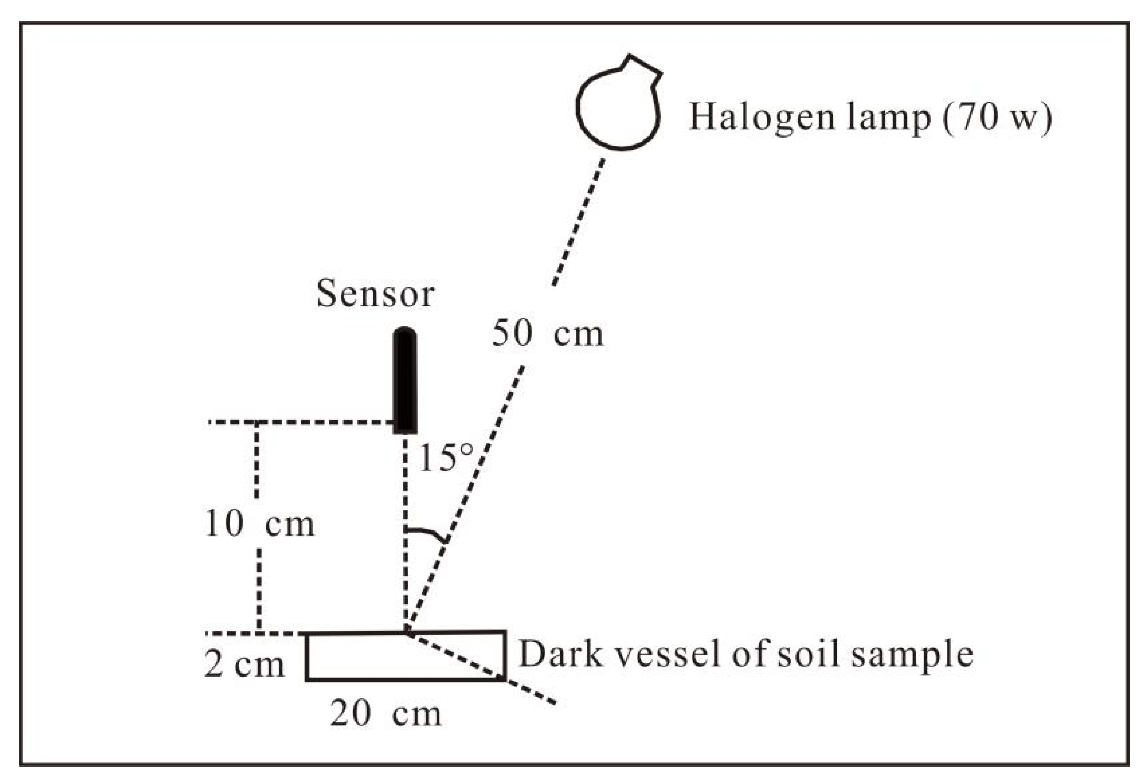
2.2.2. Laboratory Spectra Process Using Analytical Spectral Devices (ASD, USA)

In this study, the ASD FieldSpec 4 spectrometer with a wavelength range of 350–2500 nm and a resampling interval of 1 nm was used. Then, we finished the laboratory spectra measurement in a darkroom environment to obtain the ASD spectra. We first placed the sieved soil sample in a dark vessel (diameter = 20 cm, depth = 2 cm) and scraped the surface with a plastic blade (Figure 2). Then a 70 W halogen lamp was used as the light source. The distance between the light source and the soil was 50 cm, and the zenith angle was 15°. The probe was 10 cm away from the soil sample. A whiteboard was used for calibration before each measurement to eliminate the interference of dark current [51,52,53,54,55]. A total of twenty spectral curves were collected from four mutually perpendicular directions, and the average value was taken as the hyperspectral reflectance of the sample. To remove noise interference, we first removed bands (350–399 nm and 2401–2500 nm) located at a low signal-to-noise ratio (SNR) and then performed Savitzky–Golay filter transformation on hyperspectral reflectance data in the Unscrambler® X (Version 10.4, CAMO company, Oslo, Norway) [56].

2.2.3. GF-5 and HJ-1A Hyperspectral Imagery Process

Gaotai County of Hexi Corridor is located in the arid region of Northwest China. Considering the arid climate, small population density, minor surface environment change in the arid region of Northwest China, and data availability, this study used four GF-5 images accepted from 9 December 2019 to 22 January 2020 as the data source, with a swath of 60 km, a spatial resolution of 30 m, a spectral range of 400–2500 nm, and a spectral resolution of 5 nm in the visible near-infrared (VNIR) spectra and 10 nm in the short-wave infrared (SWIR) spectra. In addition, we also used nine HJ-1A images from 12 January 2018 to 21 December 2021, with a swath of 50 km, a spatial resolution of 100 m, and a spectral range of 450–950 nm (Figure 3).
In this study, PIE-Hyp software (Version 6.3, Piesat Information Technology Co., Ltd., Beijing, China) was used to preprocess 330 bands of GF-5 data (150 bands in the visible near-infrared range and 180 bands in the short-wave infrared range). The GF-5 data was downloaded from http://gaofenplatform.com/channels/4.html (accessed on 16 January 2022). First of all, it was necessary to remove the water vapour absorption bands (a total of 25 bands in two ranges: 43rd–50th band and 96th–112th band) and exclude bands in the overlapping part of the visible band and short-wave infrared band (the first four bands of the short-wave infrared band in the overlapping part). The software and instruction for hyperspectral image processing were downloaded from the software’s official website (https://www.piesat.cn/node/154, accessed on 20 March 2022). As a result, we outputted 301 bands. Then we removed vertical stripes and performed radiometric, atmospheric, and geometric correction on GF-5 data.
HJ-1A satellite hyperspectral imaging radiometer (HSI) data is a level-2 product that has undergone radiometric correction and system geometric correction. The data used in this study were downloaded from http://36.112.130.153:7777/DSSPlatform/productSearch.html (accessed on 22 January 2022). In this study, the HJ-1A/B Tools were used to import data, and the Convert Data Tool was used to convert the downloaded hyperspectral data into Band Interleaved by Pixel (BIP). The research directly removed the first twenty bands with severe noise and then used the Replace Bad Lines Tool to repair bad lines in the image, and used the Global Stripping Method and the Rotate/Flip Data Tool in the ENVI (Version 5.1, Exelis Visual Information Solutions Company, CA, USA) software to remove stripes. In ENVI, the FLAASH atmospheric correction method was used to process data, and the Select GCP: Image to Image Tool of ENVI was used to complete the geometric correction with Landsat 8 and shuttle radar topography mission (SRTM) DEM data [57,58].
To eliminate the influence of noise, this study performed Savitzky–Golay filter transformation on the GF-5 and HJ-1A hyperspectral reflectance data in the Unscrambler® X (Version 10.4, CAMO company, Oslo, Norway) [56].

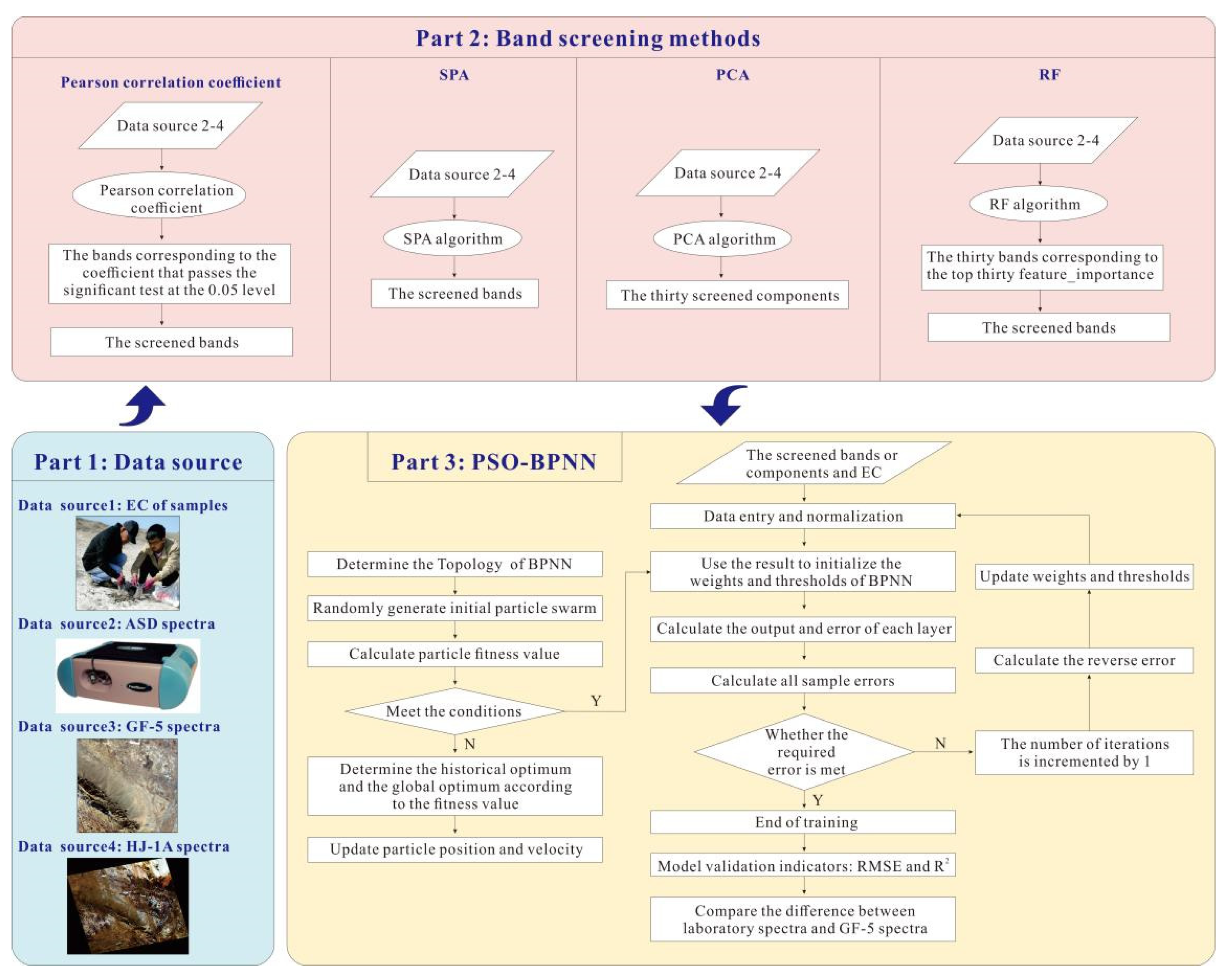
2.3. Model Establishment and Verification

The Kennard–Stone algorithm was used to select the calibration dataset and validation dataset [59]. From other studies, we can understand that the number of soil samples depends on the area of the study region [55,60], so among the 50 soil samples, 33 samples were used as the calibration dataset, and 17 samples were used as the validation dataset. The soil salinity inversion model used in this study was PSO-BPNN. The PSO algorithm code was derived from the book of Bao et al. [61]. The BPNN algorithm code was derived from neural network code in the book of Wang et al. [50,51,52,53,54,55,56,57,58,59,60,61,62]. PSO was used to optimize initial weights and thresholds of BPNN to accelerate the network convergence speed and avoid falling into local minima [63]. BPNN consists of an input layer, a hidden layer, and an output layer, and the total network error is controlled by adjusting weights [17]. In this study, the number of input layer nodes was determined by the dimension of input data (Table 1). The dimension of output data determined the number of output layer nodes. The number of hidden layer nodes was 10. The population size of PSO was 20. Band screening methods included PCC, PCA, SPA, and RF (Figure 4). The PCC for this study was performed in SPSS 23. PCA and RF were performed in PyCharm 2021.2.1 by using Python programming language (Version 3.6, Python Software Foundation, Wilmington, DE, USA). SPA and PSO-BPNN were finished in MATLAB (Version R2017a, MathWorks Inc., Natick, MA, USA).
In this study, the root mean square error (RMSE) and determination of coefficients (R2) were used to verify the model’s ability to predict EC. R2 is proportional to the simulation accuracy of models and indicates the stability of models. The RMSE is inversely proportional to the simulation accuracy of models [64].

3. Results

3.1. Descriptive Statistics of EC

The maximum, minimum, mean, median, and standard deviation (SD) of EC of all datasets were between those of calibration datasets and validation datasets, indicating that the calibration datasets could be used to establish the salinity prediction model (Table 2). The coefficient of variation (CV) of all datasets, calibration datasets, and validation datasets was large, indicating that the EC of all soil samples varied greatly.

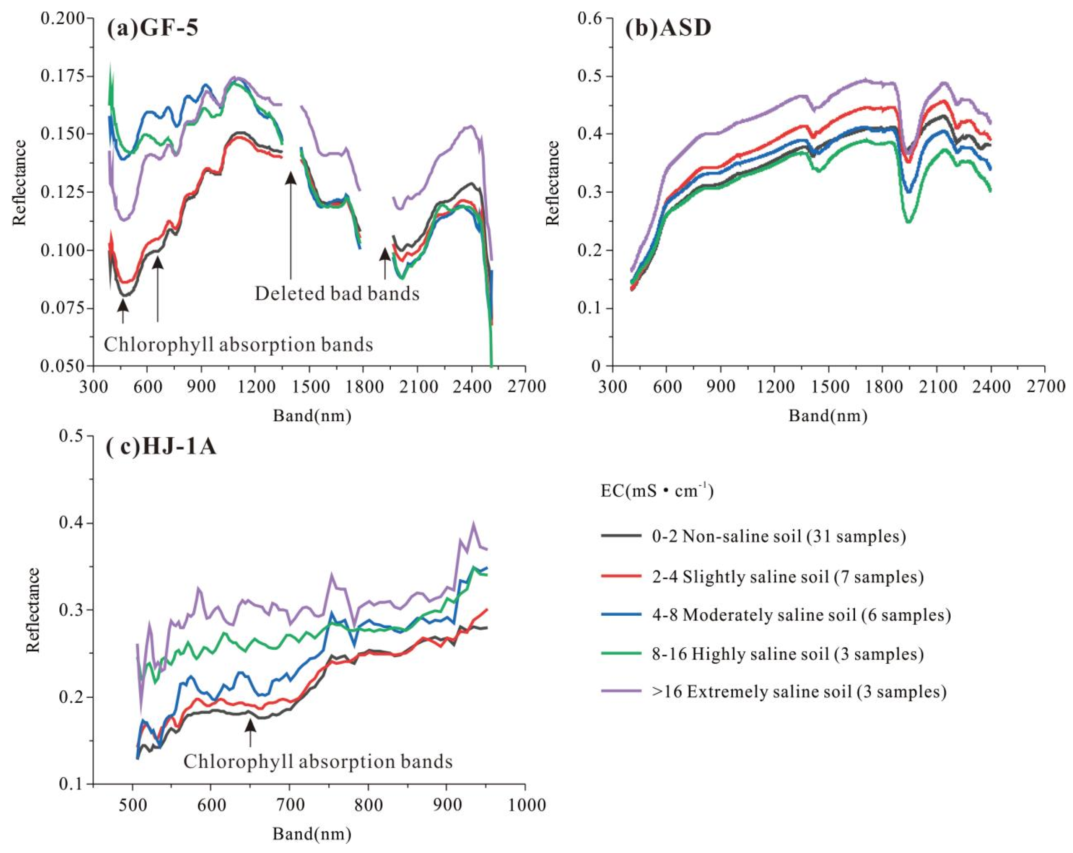
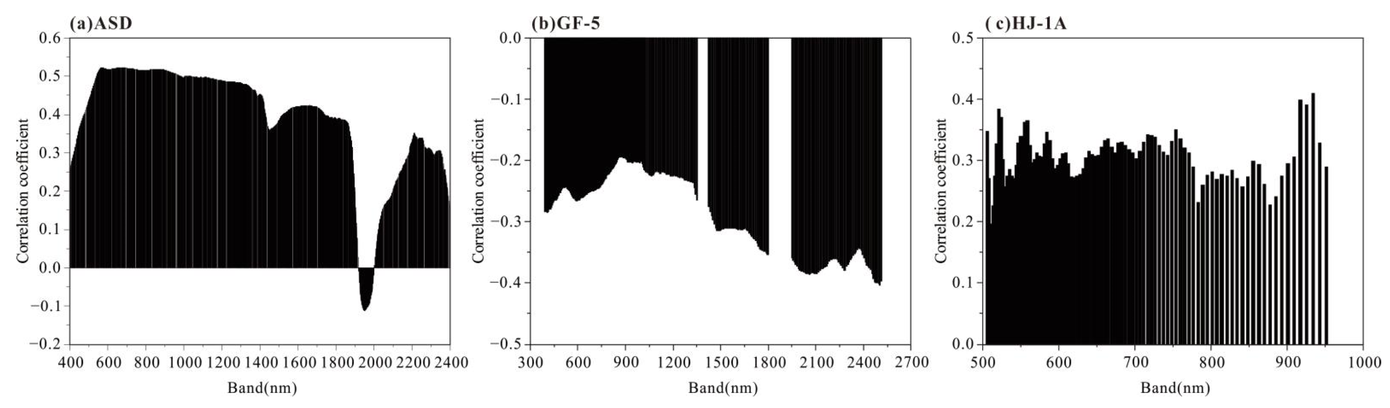
3.2. Hyperspectral Curve of Soil Samples

The slope of the ASD spectra curve in the range of 400–600 nm was high, and the reflectance increased sharply. The slope of the curve in the range of 600–1900 nm was stable. The slope of the curve in the range of 2100–2400 nm tended to decrease. Obviously, this study’s hyperspectral reflectance curve was wavy [65]. Most soil samples in the study area had water absorption valleys at approximately 1400, 1950, and 2350 nm, which were related to hydroxide ion groups in the soil (Figure 5). In this study, the hyperspectral reflectance of the extremely saline soil was much higher than that of other saline soils. Except for extremely saline soil, the difference in the hyperspectral reflectance of samples corresponding to different EC was small in this study. Possibly affected by hygroscopic water, the moderately and highly saline soils did not exhibit high reflectance. Therefore, this study used a nonlinear machine-learning algorithm to invert soil salinity.
The spatial resolution of the GF-5 hyperspectral imagery is 30 m. There might be vegetation inside the pixels of the soil sample. So, the spectral reflectance curve of soil samples was affected by vegetation in the mixed pixels. The 400–450 nm and 650–700 nm bands are chlorophyll absorption bands, and vegetation has a strong reflection in the 750–1300 nm bands. Water absorption significantly affected these bands of GF-5 data at approximately 1400 and 1950 nm, so they were deleted in this study. The GF-5 reflectance of extremely, highly, and moderately saline soil was basically higher than that of slightly saline soil and non-saline soil.
The fluctuation trend of the spectral reflectance curve of HJ-1A was similar to that of GF-5, but there was basically a positive correlation between HJ-1A and EC. With the increase of EC, the fluctuation of spectral reflectance increased.
In conclusion, the reflectance of extremely saline soil of ASD, GF-5, and HJ-1A was the highest. Compared with the reflectance curve of HJ-1A, the sample’s reflectance curve of GF-5 has relatively typical vegetation characteristics. This might have an impact on salinity inversion modeling in this study.

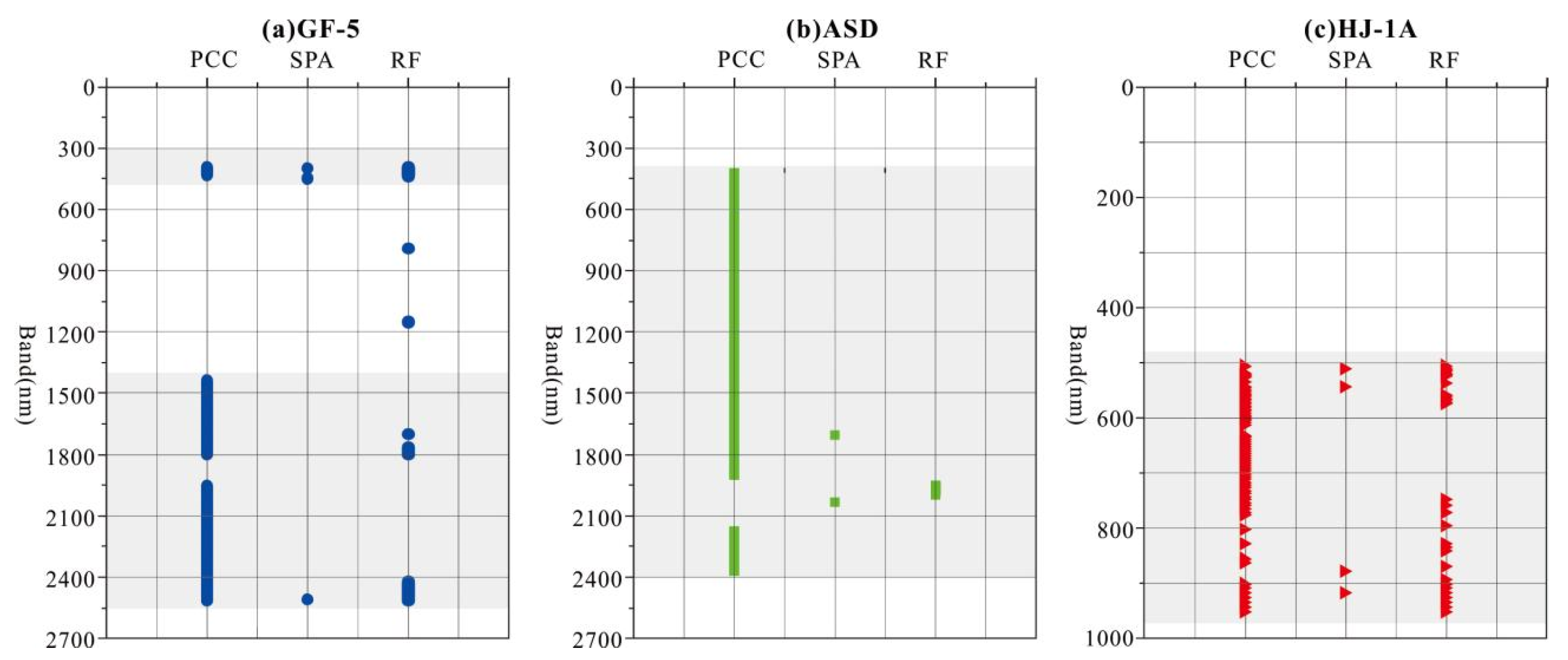
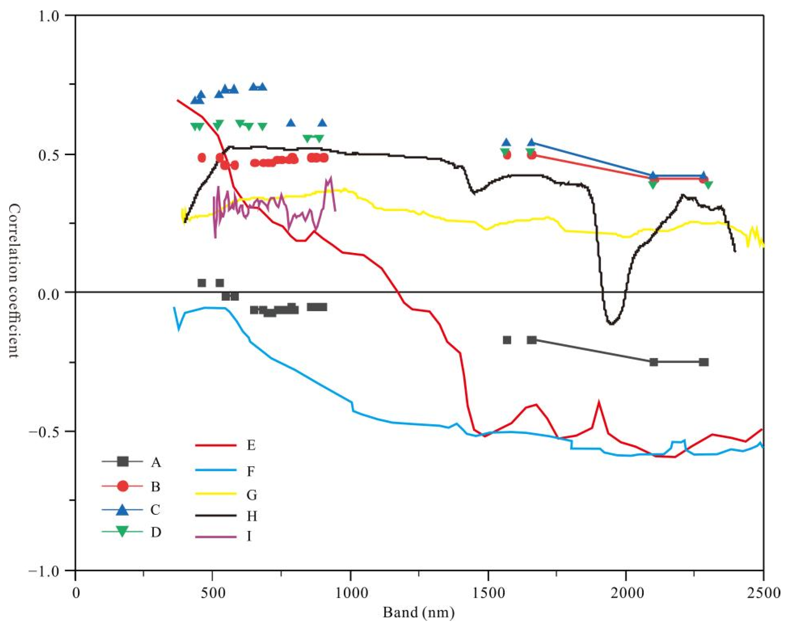
3.3. The Results of Four Band Screening Methods

In this study, all bands of ASD, GF-5, and HJ-1A that passed the significance test at 0.05 level were selected to build a soil salinity prediction model. Visible bands of ASD and HJ-1A spectra had a high correlation with EC, which showed that these bands had more soil-EC-sensitive information than GF-5 (Figure 6). The correlation between the visible band of GF-5 and EC was slightly lower than that of ASD and HJ-1A. The correlation between EC and the short-wave infrared band of GF-5 was higher than other bands. The correlation of GF-5 and HJ-1A spaceborne spectra with EC was relatively lower than that of ASD laboratory spectra, while that of GF-5 was similar to HJ-1A in general. The 2200–2650 nm bands can be used to distinguish soil texture, and soil moisture is more sensitive in 1450 and 1950 nm bands. Therefore, soil moisture can be estimated with near-infrared bands, while visible and near-infrared bands are sensitive to organic matter. Bands of 620 nm and 900 nm are sensitive to iron in the soil. So, the sensitive bands of saline soil are mainly in the range of 400–2500 nm. According to the spectral reflectance curve (Figure 6), we could find that GF-5 hyperspectral data used in this study was affected by vegetation on the soil surface, so the correlation between the reflectance of visible bands and saline soil was low, which might affect the accuracy of salinity monitoring model. The spatial resolution of GF-5 and HJ-1A is 30 m and 100 m, respectively. This study used a three-point sampling method, and the probability that one sample’s three sub-samples are located in one pixel with 30 m resolution is significantly lower than that with 100 m resolution. In this study, an ASD handheld spectrometer was used to measure the spectral reflectance of three sub-samples, which could ensure a relatively higher correlation between spectral reflectance and EC.
In the aspect of PCA, RF, and SPA, the three spectra datum in this study were treated in the same way. We set the number of principal components after dimension reduction for PCA to thirty. Principal components are linear combinations of all bands, independent of each other, but retain the main spectral information of the original bands. The bands corresponding to the top thirty importance calculated by the RF algorithm were selected for modeling in this study. The bands of HJ-1A spectra selected by RF algorithm were mainly located in the visible near-infrared band, while those of ASD were mainly located at 1800–2100 nm, indicating that these bands contain relatively rich spectral information (Figure 7). The bands of GF-5 screened by the RF did not show regular distribution characteristics. Most bands of GF-5 and HJ-1A spectra screened by SPA were located at 400–600 nm, while those of ASD were located at 1500–2100 nm. Considering the results of the four band screening methods, we could conclude that bands sensitive to soil salinity were mainly concentrated at the beginning and end of 400–2500 nm.

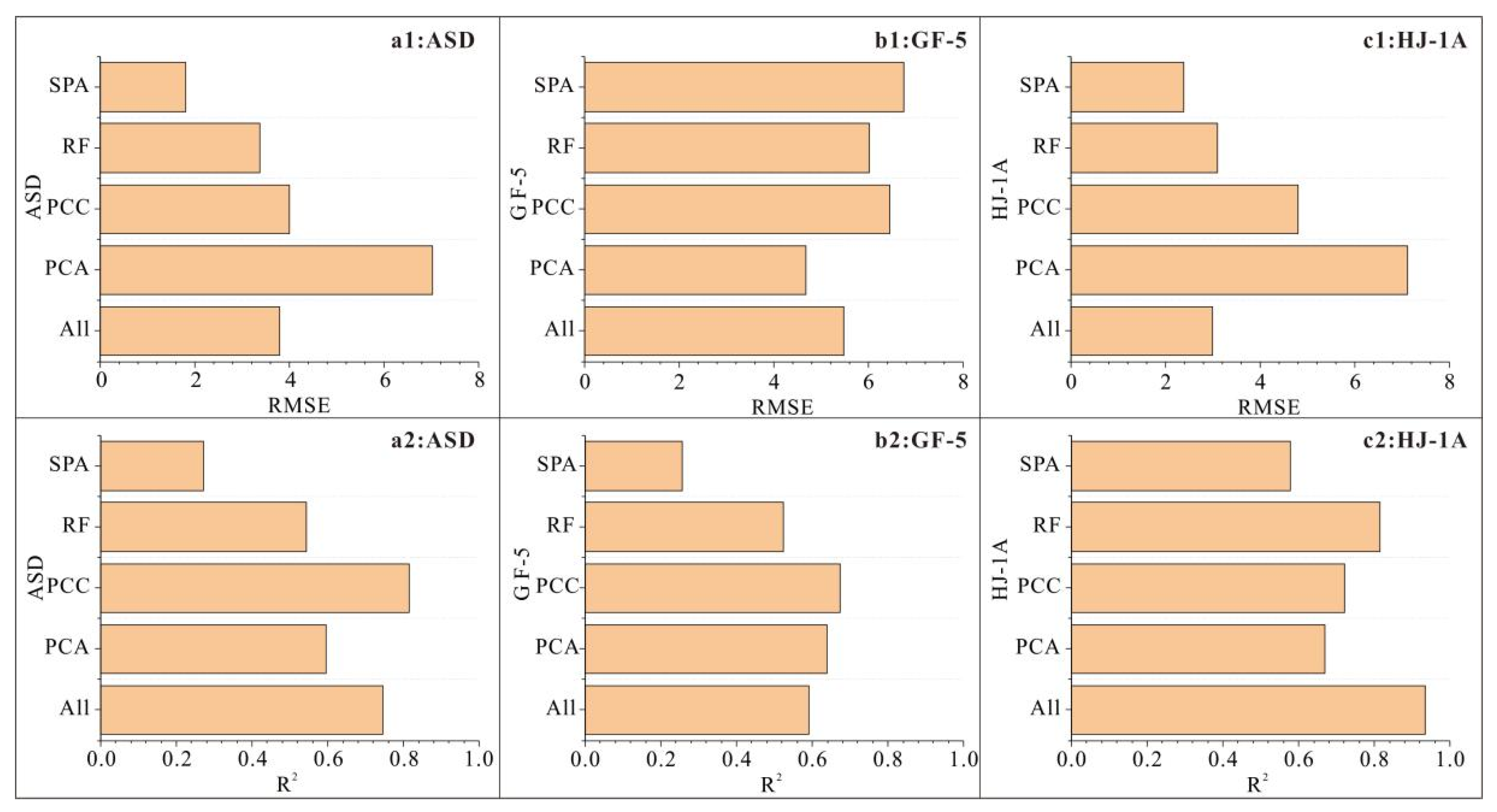
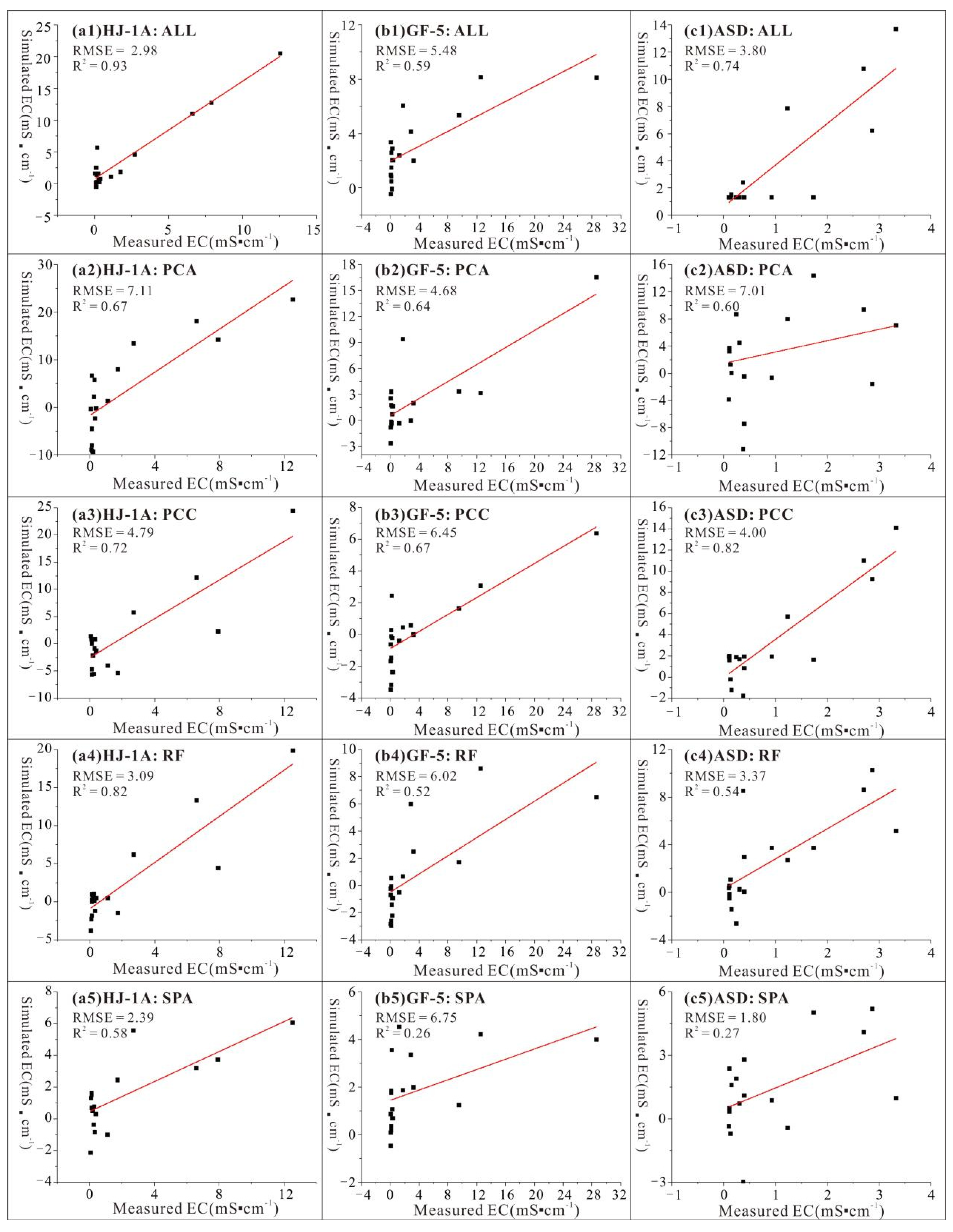
3.4. PSO-BPNN Modeling Results Based on Different Band Screening Methods

The modeling results of four band screening methods of ASD, HJ-1A, and GF-5 spectra were quite different. Overall, the best band screening method for ASD and GF-5 spectra was PCC, and the worst was SPA (Figure 8). The best band screening method of HJ-1A spectra was RF, and the worst was SPA. The model based on the PCC band screening method had the most stable performance, in general. The mean values of all model validation indicators of ASD and HJ-1A spectra were similar. The result of HJ-1A spectra was relatively better than that of GF-5 spectra in the salinity monitoring, which might be due to the influence of vegetation as well as the mismatch between sub-samples of one sample and pixel in GF-5 imagery. The good result of GF-5 and HJ-1A proved the potential and feasibility of these spectra to map soil salinity.
The PSO-BPNN that had the best simulation accuracy for ASD spectra was based on bands selected by PCC, whose RMSE and R2 were 4.00 mS·cm−1 and 0.82, respectively. The model that had the best simulation accuracy for HJ-1A spectra was based on all bands without band screening method, the RMSE and R2 of which were 2.98 mS·cm−1 and 0.93, respectively. The model that had the best simulation accuracy for GF-5 spectra was based on bands selected by PCC, and its RMSE and R2 were 6.45 mS·cm−1 and 0.67, respectively (Figure 9). These indicated that PCC was the most suitable and robust band screening method for PSO-BPNN to predict EC in the study area and that the prediction accuracy of the model was basically improved after dimension reduction by using the band screening method in most cases.

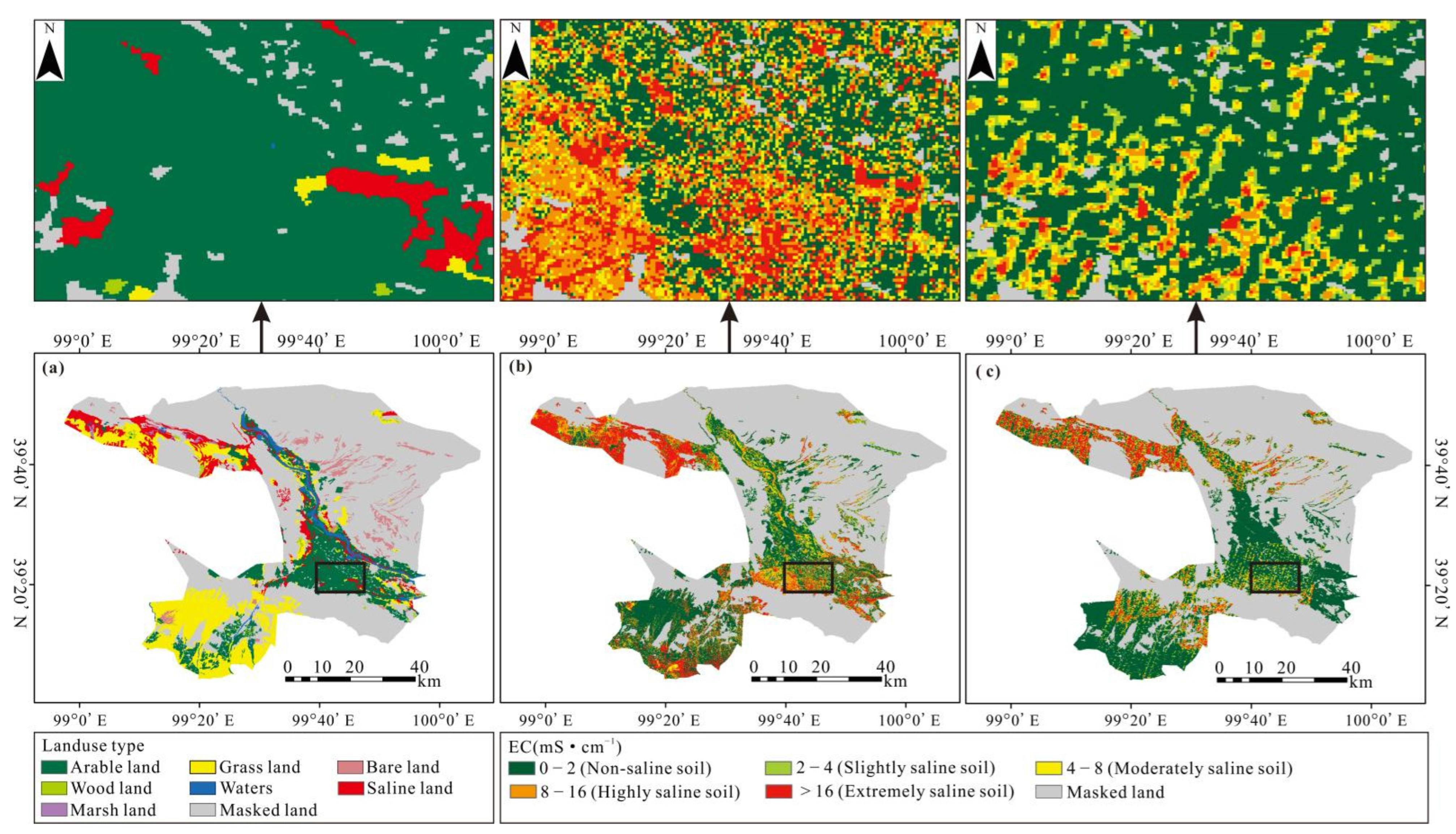
3.5. Distribution of Saline Soil in Gaotai County

It was found that the performance of PCC-PSO-BPNN was best for GF-5 spectra. Therefore, the PCC-PSO-BPNN model was used to map the soil salinity distribution in the study area with GF-5 spectra. When all bands of HJ-1A were used to build the PSO-BPNN model, the salinity monitoring result was the best. So, we used the PSO-BPNN model with all bands of HJ-1A spectra to map soil salinity distribution. We inputted GF-5 and HJ-1A remote sensing images into the optimal model saved in the MATLAB platform to obtain the distribution map of soil salinity.
From the result, we could verify that the signal-to-noise ratio and spatial resolution of GF-5 were better than that of HJ-1A. The detailed spectral information of GF-5 spectra was more abundant than that of HJ-1A (Figure 10). Yin et al. proved that GF-5 spectra with a high spectral resolution, good signal-to-noise ratio, and wide swath coverage could provide convenience for quick and large-scale soil salinity monitoring [67]. However, the simulation accuracy of the PSO-BPNN model based on HJ-1A was relatively higher than that of GF-5, with a better signal-to-noise ratio, which indicated that PSO-BPNN had a strong ability to deal with noise.
The distribution of saline soil predicted by GF-5 and HJ-1A was similar (Figure 10). The results of HJ-1A showed that most arable lands were moderately, highly, and extremely saline soil. The map derived from GF-5 indicated that most arable lands were highly and extremely saline soil. The prediction results of these two spaceborne hyperspectral data showed that the saline soil in arable land was distributed in patches, mainly in the south of arable land. The northwest grassland in Gaotai County was basically extremely saline soil. Some grasslands in southwest Gaotai County were highly and extremely saline soil. The other unmasked land in Gaotai County belonged to non-saline and slightly saline soil.

4. Discussion

4.1. Comparative Analysis of Different Data Sources

The performance of models established by ASD, HJ-1A, and GF-5 spectra in this study was relatively good, and models of ASD and HJ-1A spectra performed better than those of the GF-5 spectra. Other studies obtained similar results. Yin et al. used ASD laboratory spectra as well as GF-5 spectra to predict soil copper content with a piecewise partial least square regression (P-PLSR) model, and found that the inversion accuracy of the former was slightly better than that of the latter [67]. Hong et al. reached a similar result [68]. The spectral reflectance curve indicated that soil samples of this study in GF-5 imagery were affected by vegetation. The GF-5 spectral reflectance curve of samples has relatively obvious vegetation characteristics. In addition, the spatial resolution of HJ-1A and GF-5 hyperspectral imagery is 100 m and 30 m, respectively. We used a three-point sampling method in this study, which might affect the matching degree between one sample’s three sub-samples and pixel of spaceborne HJ-1A and GF-5 hyperspectral imagery, thus affecting the performance of models.
At present, many studies have carried out comparative analyses of data sources with different spectral and spatial resolutions. Hyperspectral data characterized by large data volume and multicollinearity usually contains three types of spectral data: effective data, redundant data, and non-informative data [69]. Lu et al. compared the performance of multispectral and hyperspectral images in estimating the chlorophyll content of vegetation and found that the predictive ability of the hyperspectral image was slightly better than that of the multispectral image, but its redundant bands could not significantly improve the model performance [70]. Therefore, we used PCC, RF, SPA, and PCA to reduce the dimension of hyperspectral data and found that the accuracy of the model coupled with the band screening method was improved. Hong et al. used continuous wavelet transform (CWT) and competitive adaptive reweighted sampling (CARS) to screen airborne hyperspectral imagery and ASD spectra, and used the RF algorithm to predict soil organic carbon, and found that the ASD spectra had a better result than airborne hyperspectral imagery (Table 3) [68]. Wang et al. established a soil salinity estimation model based on hyperspectral data and multispectral data, and found that the hyperspectral model was slightly better than the multispectral model [71]. However, Shruti Khanna et al. compared three multispectral satellite sensors (WorldView2, RapidEye, and Landsat EMT+) with the aerial hyperspectral AVIRIS sensor and found that spectral resolution was not as strong as the spatial resolution in improving the detection and mapping of oil-impacted wetlands, suggesting that broadband data with high spatial resolution might be sufficient to detect oil-impacted wetlands [23]. Therefore, in the future, we may use multispectral data with a higher spatial resolution to carry out comparative research.

4.2. Spatial Distribution Mapping of Soil Salinity

Remote sensing technology has been widely used in soil salinity prediction for a long time [66]. Both indoor and field spectra can only provide point-to-point data and are not suitable for continuous prediction and mapping of the soil content [72,73]. Many studies have used measurement results of field samples to study the distribution of saline soil, while few have upscaled the estimation models to airborne or spaceborne imagery [74]. Spaceborne hyperspectral sensors with higher spectral resolution have increased the potential for the prediction of soil content [75]. However, due to the differences in the surface environment in different regions, there is no widely applicable soil salinity monitoring model, and the existing research is mainly based on the local scale [76,77,78]. Gaotai County, in the middle reaches of the Heihe River basin, is a typical salinization area in the Hexi Corridor. We obtained relatively good salinity monitoring results in Gaotai County when using spaceborne satellite hyperspectral data to predict soil salinity, which indicated that HJ-1A and GF-5 might be suitable for soil salinity mapping in this area in the future.

4.3. Analysis of the Sensitive Bands of Soil Salinization

This study showed that bands of hyperspectral data had a large amount of information sensitive to soil salinity at the beginning and end of 400–2500 nm bands. Wang et al. proved that soil salt content had high correlations with bands at the beginning and final wavelengths and had low coefficients with bands in the middle wavelengths of laboratory hyperspectral reflectance data (400–2500 nm) (Figure 11) [51]. The laboratory hyperspectral band at 2257 nm among bands from 400 to 2500 nm showed the highest correlation with EC [5]. The other remote sensing imagery had a similar result. Wang et al. proved that bands 1–4 of Landsat 8 OLI and Sentinel-2 MSI had a good correlation with soil salinity, while the latter was more sensitive to soil salinity than the former [79]. Zhou et al. found that all bands of Sentinel-2A multispectral remote sensing images were not related to soil salinity, and the highest correlation was 0.24 [80], which might be caused by the complexity of soil structure and surface environment. However, in another study, the reflectance data of all bands of Sentinel-2A data exhibited a positive correlation with soil salt content; band 2 (490 nm), band 8 (842 nm), band 8a (865 nm), band 11 (1610 nm), and band 12 (2190 nm) were significantly correlated with soil salt content [81]. Band 2 and band 12 were located at the head and tail of 400–2500 nm. This was basically consistent with the conclusion of our study.

4.4. Applicability of Machine Learning Algorithms

In this study, we built a PSO-BPNN model based on PCC, PCA, SPA, and RF, and obtained optimal results. The simulation accuracy of the PSO-BPNN model, whose data source was HJ-1A, was higher than the model based on GF-5 with good spatial resolution and signal-to-noise ratio, which indicated that PSO-BPNN had a strong ability to deal with noise. Other studies based on machine learning methods had similar results [82,83,84] (Table 4). Wei et al. proposed the particle swarm optimization–support vector machine regression (PSO-SVR) and PSO-BPNN models to study soil salinity and found that the prediction accuracy of PSO-BPNN and PSO-SVR was better than that of BPNN and SVR [19]. Fu et al. built a particle swarm optimization–probability neural network (PSO-PNN) model to study soil salt content and proved that this model had excellent predictive power [85].

5. Conclusions

Soil salinization problems occur in many arid regions around the world. A large number of studies focus on ground hyperspectral or spaceborne multispectral data, and few studies compare the spaceborne hyperspectral image and ground hyperspectral data in soil salinity monitoring. Therefore, we chose Gaotai County of Hexi Corridor in Northwestern China as the study area. Soil salinity inversion models (PCC-PSO-BPNN, PCA-PSO-BPNN, SPA-PSO-BPNN, RF-PSO-BPNN, and PSO-BPNN without band screening method) were established to compare the applicability of ASD, HJ-1A, and GF-5 spectra in soil salinity monitoring, and carry out the study of the distribution of different saline soils. The initial weights and thresholds of the BPNN algorithm are random, and the PSO algorithm improves this shortcoming.
The band screening methods in this study showed that bands at the beginning and end of 400–2500 nm had a higher correlation with EC, and have more sensitive soil information. In general, the overall performance of PCC-PSO-BPNN was more stable and robust. The band screening method might improve the accuracy of the model. The mean results of models for HJ-1A spectra were relatively better than those for the GF-5 spectra, with good spatial resolution and signal-to-noise ratio. This indicated that PSO-BPNN could effectively deal with noise. The different matching degree between one sample’s three sub-samples and pixels of GF-5 and HJ-1A imagery might be another reason for the result. The soil reflectance curve showed that GF-5 might be influenced by vegetation. The probability that one sample’s three sub-samples were located in a pixel with a resolution of 30 m (GF-5) was much lower than that in a pixel with a resolution of 100 m (HJ-1A).
The soil salinity distribution map based on HJ-1A and GF-5 showed that the extremely and highly saline soil in Gaotai County was mainly distributed in grassland and arable land. Other unmasked lands mainly featured non-saline and slightly saline soil. This study analyzed the difference in the ability of soil salinity prediction among GF-5, ASD, and HJ-1A spectra, and did not study different multispectral data sources, which will be studied in future research.

Author Contributions

X.J. completed the field sampling, laboratory experiment, formal analysis, and manuscript writing. X.X. helped design the field work and revise the manuscript. All authors have read and agreed to the published version of the manuscript.

Funding

This work was supported by the Second Tibetan Plateau Scientific Expedition and Research Program (2019QZKK0305).

Data Availability Statement

The GF-5 data was from http://gaofenplatform.com/channels/4.html (accessed on 16 January 2022). The PIE-Hyp software was from https://www.piesat.cn/node/154 (accessed on 20 March 2022). The HJ-1A data was from http://36.112.130.153:7777/DSSPlatform/productSearch.html (accessed on 22 January 2022). The land use data was from https://www.resdc.cn/Default.aspx (accessed on 30 January 2022).

Conflicts of Interest

The authors declare no conflict of interest.

References

  1. Hopmans, J.W.; Qureshi, A.S.; Kisekka, I.; Munns, R.; Grattan, S.R.; Rengasamy, P.; Ben-Gal, A.; Assouline, S.; Javaux, M.; Minhas, P.S. Advances in Agronomy; Academic Press: Pittsburgh, PA, USA, 2021. [Google Scholar]
  2. Salcedo, F.P.; Cutillas, P.P.; Cabañero, J.J.A.; Vivaldi, A.G. Use of remote sensing to evaluate the effects of environmental factors on soil salinity in a semi-arid area. Sci. Total Environ. 2022, 815, 152524. [Google Scholar] [CrossRef]
  3. Zhu, K.; Sun, Z.; Zhao, F.; Yang, T.; Tian, Z.; Lai, J.; Zhu, W.; Long, B. Relating Hyperspectral Vegetation Indices with Soil Salinity at Different Depths for the Diagnosis of Winter Wheat Salt Stress. Remote Sens. 2021, 13, 250. [Google Scholar] [CrossRef]
  4. Singh, A. Soil salinization management for sustainable development: A review. J. Environ. Manag. 2021, 277, 111383. [Google Scholar] [CrossRef] [PubMed]
  5. Mashimbye, Z.E.; Cho, M.A.; Nell, J.P.; De Clercq, W.P.; Van Niekerk, A.; Turner, D.P. Model-Based Integrated Methods for Quantitative Estimation of Soil Salinity from Hyperspectral Remote Sensing Data: A Case Study of Selected South African Soils. Pedosphere 2012, 22, 640–649. [Google Scholar] [CrossRef]
  6. Wu, W.; Zucca, C.; Muhaimeed, A.S.; Al-Shafie, W.M.; Fadhil Al-Quraishi, A.M.; Nangia, V.; Zhu, M.; Liu, G. Soil salinity prediction and mapping by machine learning regression in Central Mesopotamia, Iraq. Land Degrad. Dev. 2018, 29, 4005–4014. [Google Scholar] [CrossRef]
  7. Ma, L.; Yang, S.; Simayi, Z.; Gu, Q.; Li, J.; Yang, X.; Ding, J. Modeling variations in soil salinity in the oasis of Junggar Basin, China. Land Degrad. Dev. 2018, 29, 551–562. [Google Scholar] [CrossRef]
  8. Xu, H.; Chen, C.; Zheng, H.; Luo, G.; Yang, L.; Wang, W.; Wu, S.; Ding, J. AGA-SVR-based selection of feature subsets and optimization of parameter in regional soil salinization monitoring. Int. J. Remote Sens. 2020, 41, 4470–4495. [Google Scholar] [CrossRef]
  9. Fathizad, H.; Ali Hakimzadeh Ardakani, M.; Sodaiezadeh, H.; Kerry, R.; Taghizadeh-Mehrjardi, R. Investigation of the spatial and temporal variation of soil salinity using random forests in the central desert of Iran. Geoderma 2020, 365, 114233. [Google Scholar] [CrossRef]
  10. Figueiredo, E.M.N.; Ludermir, T.B. Investigating the use of alternative topologies on performance of the PSO-ELM. Neurocomputing 2014, 127, 4–12. [Google Scholar] [CrossRef]
  11. Lin, S.; Ying, K.; Chen, S.; Lee, Z. Particle swarm optimization for parameter determination and feature selection of support vector machines. Expert Syst. Appl. 2008, 35, 1817–1824. [Google Scholar] [CrossRef]
  12. Wei, J.; Jian-qi, Z.; Xiang, Z. Face recognition method based on support vector machine and particle swarm optimization. Expert Syst. Appl. 2011, 38, 4390–4393. [Google Scholar] [CrossRef]
  13. Zhang, X.; Chen, X.; He, Z. An ACO-based algorithm for parameter optimization of support vector machines. Expert Syst. Appl. 2010, 37, 6618–6628. [Google Scholar] [CrossRef]
  14. Li, L.; Sun, J.; Tseng, M.; Li, Z. Extreme learning machine optimized by whale optimization algorithm using insulated gate bipolar transistor module aging degree evaluation. Expert Syst. Appl. 2019, 127, 58–67. [Google Scholar] [CrossRef]
  15. Ab Aziz, M.F.; Mostafa, S.A.; Foozy, C.F.M.; Mohammed, M.A.; Elhoseny, M.; Abualkishik, A.Z. Integrating Elman recurrent neural network with particle swarm optimization algorithms for an improved hybrid training of multidisciplinary datasets. Expert Syst. Appl. 2021, 183, 115441. [Google Scholar] [CrossRef]
  16. Kushwah, R.; Kaushik, M.; Chugh, K. A modified whale optimization algorithm to overcome delayed convergence in artificial neural networks. Soft Comput. 2021, 25, 10275–10286. [Google Scholar] [CrossRef]
  17. Liu, X.; Liu, Z.; Liang, Z.; Zhu, S.; Correia, J.A.F.O.; De Jesus, A.M.P. PSO-BP Neural Network-Based Strain Prediction of Wind Turbine Blades. Materials 2019, 12, 1889. [Google Scholar] [CrossRef] [Green Version]
  18. Das, B.; Manohara, K.K.; Mahajan, G.R.; Sahoo, R.N. Spectroscopy based novel spectral indices, PCA- and PLSR-coupled machine learning models for salinity stress phenotyping of rice. Spectrochim. Acta Part A Mol. Biomol. Spectrosc. 2020, 229, 117983. [Google Scholar] [CrossRef]
  19. Wei, Q.; Nurmemet, I.; Gao, M.; Xie, B. Inversion of Soil Salinity Using Multisource Remote Sensing Data and Particle Swarm Machine Learning Models in Keriya Oasis, Northwestern China. Remote Sens. 2022, 14, 512. [Google Scholar] [CrossRef]
  20. Daniel, K.W.; Tripathi, N.K.; Honda, K. Artificial neural network analysis of laboratory and in situ spectra for the estimation of macronutrients in soils of Lop Buri (Thailand). Soil Res. 2003, 41, 47–59. [Google Scholar] [CrossRef]
  21. Yu, X.; Chang, C.; Song, J.; Zhuge, Y.; Wang, A. Precise Monitoring of Soil Salinity in China’s Yellow River Delta Using UAV-Borne Multispectral Imagery and a Soil Salinity Retrieval Index. Sensors 2022, 22, 546. [Google Scholar] [CrossRef]
  22. Taghadosi, M.M.; Hasanlou, M.; Eftekhari, K. Soil salinity mapping using dual-polarized SAR Sentinel-1 imagery. Int. J. Remote Sens. 2019, 40, 237–252. [Google Scholar] [CrossRef]
  23. Zhang, Q.; Li, L.; Sun, R.; Zhu, D.; Zhang, C.; Chen, Q. Retrieval of the Soil Salinity from Sentinel-1 Dual-Polarized SAR Data Based on Deep Neural Network Regression. IEEE Geosci. Remote Sens. Lett. 2020, 19, 4006905. [Google Scholar] [CrossRef]
  24. Ma, Y.; Chen, H.; Zhao, G.; Wang, Z.; Wang, D. Spectral Index Fusion for Salinized Soil Salinity Inversion Using Sentinel-2A and UAV Images in a Coastal Area. IEEE Access 2020, 8, 159595–159608. [Google Scholar] [CrossRef]
  25. Khanna, S.; Maria, J.S.; Ustin, S.L.; Shapiro, K.; Haverkamp, P.J.; Lay, M. Comparing the Potential of Multispectral and Hyperspectral Data for Monitoring Oil Spill Impact. Sensors 2018, 18, 558. [Google Scholar] [CrossRef] [PubMed] [Green Version]
  26. van Wagtendonk, J.W.; Root, R.R.; Key, C.H. Comparison of AVIRIS and Landsat ETM+ detection capabilities for burn severity. Remote Sens. Environ. 2004, 92, 397–408. [Google Scholar] [CrossRef]
  27. Teillet, P.M.; Staenz, K.; William, D.J. Effects of spectral, spatial, and radiometric characteristics on remote sensing vegetation indices of forested regions. Remote Sens. Environ. 1997, 61, 139–149. [Google Scholar] [CrossRef]
  28. Bai, L.; Wang, C.; Zang, S.; Wu, C.; Luo, J.; Wu, Y. Mapping Soil Alkalinity and Salinity in Northern Songnen Plain, China with the HJ-1 Hyperspectral Imager Data and Partial Least Squares Regression. Sensors 2018, 18, 3855. [Google Scholar] [CrossRef] [Green Version]
  29. Weng, Y.; Gong, P.; Zhu, Z. A Spectral Index for Estimating Soil Salinity in the Yellow River Delta Region of China Using EO-1 Hyperion Data. Pedosphere 2010, 20, 378–388. [Google Scholar] [CrossRef]
  30. Hu, J.; Peng, J.; Zhou, Y.; Xu, D.; Zhao, R.; Jiang, Q.; Fu, T.; Wang, F.; Shi, Z. Quantitative Estimation of Soil Salinity Using UAV-Borne Hyperspectral and Satellite Multispectral Images. Remote Sens. 2019, 11, 736. [Google Scholar] [CrossRef] [Green Version]
  31. Hbirkou, C.; Pätzold, S.; Mahlein, A.; Welp, G. Airborne hyperspectral imaging of spatial soil organic carbon heterogeneity at the field-scale. Geoderma 2012, 175–176, 21–28. [Google Scholar] [CrossRef]
  32. Nouri, M.; Gomez, C.; Gorretta, N.; Roger, J.M. Clay content mapping from airborne hyperspectral Vis-NIR data by transferring a laboratory regression model. Geoderma 2017, 298, 54–66. [Google Scholar] [CrossRef]
  33. Lin, L.; Gao, Z.; Liu, X. Estimation of soil total nitrogen using the synthetic color learning machine (SCLM) method and hyperspectral data. Geoderma 2020, 380, 114664. [Google Scholar] [CrossRef]
  34. Pfitzner, K.S.; Harford, A.J.; Whiteside, T.G.; Bartolo, R.E. Mapping magnesium sulfate salts from saline mine discharge with airborne hyperspectral data. Sci. Total Environ. 2018, 640–641, 1259–1271. [Google Scholar] [CrossRef]
  35. Ghamisi, P.; Couceiro, M.S.; Martins, F.M.L.; Benediktsson, J.A. Multilevel Image Segmentation Based on Fractional-Order Darwinian Particle Swarm Optimization. IEEE Trans. Geosci. Remote Sens. 2014, 52, 2382–2394. [Google Scholar] [CrossRef] [Green Version]
  36. Hong, Y.; Liu, Y.; Chen, Y.; Liu, Y.; Yu, L.; Liu, Y.; Cheng, H. Application of fractional-order derivative in the quantitative estimation of soil organic matter content through visible and near-infrared spectroscopy. Geoderma 2019, 337, 758–769. [Google Scholar] [CrossRef]
  37. Tian, A.; Zhao, J.; Xiong, H.; Gan, S.; Fu, C. Application of Fractional Differential Calculation in Pretreatment of Saline Soil Hyperspectral Reflectance Data. J. Sens. 2018, 2018, 8017614. [Google Scholar] [CrossRef]
  38. Wang, X.; Zhang, F.; Kung, H.; Johnson, V.C. New methods for improving the remote sensing estimation of soil organic matter content (SOMC) in the Ebinur Lake Wetland National Nature Reserve (ELWNNR) in northwest China. Remote Sens. Environ. 2018, 218, 104–118. [Google Scholar] [CrossRef]
  39. Nawar, S.; Buddenbaum, H.; Hill, J.; Kozak, J. Modeling and Mapping of Soil Salinity with Reflectance Spectroscopy and Landsat Data Using Two Quantitative Methods (PLSR and MARS). Remote Sens. 2014, 6, 10813–10834. [Google Scholar] [CrossRef] [Green Version]
  40. Meng, L.; Zhou, S.; Zhang, H.; Bi, X. Estimating soil salinity in different landscapes of the Yellow River Delta through Landsat OLI/TIRS and ETM+ Data. J. Coast. Conserv. 2016, 20, 271–279. [Google Scholar] [CrossRef]
  41. Wang, F.; Yang, S.; Wei, Y.; Shi, Q.; Ding, J. Characterizing soil salinity at multiple depth using electromagnetic induction and remote sensing data with random forests: A case study in Tarim River Basin of southern Xinjiang, China. Sci. Total Environ. 2021, 754, 142030. [Google Scholar] [CrossRef]
  42. Shi, H.; Hellwich, O.; Luo, G.; Chen, C.; He, H.; Ochege, F.U.; Van de Voorde, T.; Kurban, A.; de Maeyer, P. A Global Meta-Analysis of Soil Salinity Prediction Integrating Satellite Remote Sensing, Soil Sampling, and Machine Learning. IEEE Trans. Geosci. Remote Sens. 2021, 60, 4505815. [Google Scholar] [CrossRef]
  43. Ding, Y.X.; Peng, S.Z. Spatiotemporal trends and attribution of drought across China from 1901–2100. Sustainability 2020, 12, 477. [Google Scholar] [CrossRef] [Green Version]
  44. Ding, Y.X.; Peng, S.Z. Spatiotemporal change and attribution of potential evapotranspiration over China from 1901 to 2100. Theor. Appl. Climatol. 2021, 145, 79–94. [Google Scholar] [CrossRef]
  45. Peng, S.Z.; Gang, C.; Cao, Y.; Chen, Y.M. Assessment of climate change trends over the loess plateau in China from 1901 to 2100. Int. J. Climatol. 2017, 38, 2250–2264. [Google Scholar] [CrossRef]
  46. Peng, S.Z.; Ding, Y.X.; Liu, W.Z.; Li, Z. 1 km monthly temperature and precipitation dataset for China from 1901 to 2017. Earth Syst. Sci. Data 2019, 11, 1931–1946. [Google Scholar] [CrossRef] [Green Version]
  47. Peng, S.Z. 1 km Monthly Potential Evapotranspiration Dataset in China (1990–2021); National Tibetan Plateau Data Center: Beijing, China, 2022. [Google Scholar]
  48. Peng, S.Z. 1-km Monthly Maximum Temperature Dataset for China (1901–2021); National Tibetan Plateau Data Center: Beijing, China, 2020. [Google Scholar]
  49. Peng, S.Z. 1-km Monthly Precipitation Dataset for China (1901–2021); National Tibetan Plateau Data Center: Beijing, China, 2020. [Google Scholar]
  50. Peng, S.Z.; Ding, Y.X.; Wen, Z.M.; Chen, Y.M.; Cao, Y.; Ren, J.Y. Spatiotemporal change and trend analysis of potential evapotranspiration over the Loess Plateau of China during 2011–2100. Agric. For. Meteorol. 2020, 233, 183–194. [Google Scholar] [CrossRef] [Green Version]
  51. Wang, Q.; Li, P.; Chen, X. Modeling salinity effects on soil reflectance under various moisture conditions and its inverse application: A laboratory experiment. Geoderma 2012, 170, 103–111. [Google Scholar] [CrossRef]
  52. Adeline, K.R.M.; Gomez, C.; Gorretta, N.; Roger, J.M. Predictive ability of soil properties to spectral degradation from laboratory Vis-NIR spectroscopy data. Geoderma 2017, 288, 143–153. [Google Scholar] [CrossRef] [Green Version]
  53. Farifteh, J.; van der Meer, F.; van der Meijde, M.; Atzberger, C. Spectral characteristics of salt-affected soils: A laboratory experiment. Geoderma 2008, 145, 196–206. [Google Scholar] [CrossRef]
  54. Tian, Y.; Zhang, J.; Yao, X.; Cao, W.; Zhu, Y. Laboratory assessment of three quantitative methods for estimating the organic matter content of soils in China based on visible/near-infrared reflectance spectra. Geoderma 2013, 202–203, 161–170. [Google Scholar] [CrossRef]
  55. Nawar, S.; Buddenbaum, H.; Hill, J.; Kozak, J.; Mouazen, A.M. Estimating the soil clay content and organic matter by means of different calibration methods of vis-NIR diffuse reflectance spectroscopy. Soil Tillage Res. 2016, 155, 510–522. [Google Scholar] [CrossRef] [Green Version]
  56. Savitzky, A.; Golay, M.J. Smoothing and differentiation of data by simplified least squares procedures. Anal. Chem. 1964, 36, 1627–1639. [Google Scholar] [CrossRef]
  57. Tian, H.; Cao, C.; Xu, M.; Zhu, Z.; Liu, D.; Wang, X.; Cui, S. Estimation of chlorophyll-a concentration in coastal waters with HJ-1A HSI data using a three-band bio-optical model and validation. Int. J. Remote Sens. 2014, 35, 5984–6003. [Google Scholar] [CrossRef]
  58. Yan, J.; Zhou, K.; Liu, D.; Wang, J.; Wang, L.; Liu, H. Alteration information extraction using improved relative absorption band-depth images, from HJ-1A HSI data: A case study in Xinjiang Hatu gold ore district. Int. J. Remote Sens. 2014, 35, 6728–6741. [Google Scholar] [CrossRef]
  59. Kennard, R.W.; Stone, L.A. Computer aided design of experiments. Technometrics 1969, 11, 137–148. [Google Scholar] [CrossRef]
  60. Wang, J.; Wang, W.; Hu, Y.; Tian, S.; Liu, D. Soil Moisture and Salinity Inversion Based on New Remote Sensing Index and Neural Network at a Salina-Alkaline Wetland. Water 2021, 13, 2762. [Google Scholar] [CrossRef]
  61. Bao, Z.Y.; Yu, J.Z.; Yang, S. Intelligent Optimization Algorithm and Its MATLAB Example; Electronics Industry Press: Beijing, China, 2018. [Google Scholar]
  62. Wang, X.C.; Shi, F.; Yu, L.; Li, Y. Analysis of 43 Cases of Neural Network in MATLAB; Beihang University Press: Beijing, China, 2013. [Google Scholar]
  63. Norouz, M. Visual-Inertial State Estimation Based on PSO-BPNN UKF. In Proceedings of the 2020 28th Iranian Conference on Electrical Engineering (ICEE), Tabriz, Iran, 4–6 August 2020; IEEE: New York, NY, USA, 2020. [Google Scholar]
  64. Shi, Z.; Wang, Q.L.; Peng, J.; Ji, W.J.; Liu, H.X.; Li, X.; Rossel, R.A.V. Development of a national VNIR soil-spectral library for soil classification and prediction of organic matter concentrations. Sci. China Earth Sci. 2014, 44, 978–988. [Google Scholar] [CrossRef]
  65. Dai, C.D.; Jiang, X.G.; Tang, L.L. Application Processing and Analysis of Remote Sensing Image; Tsinghua University Press: Beijing, China, 2003. [Google Scholar]
  66. Ivushkin, K.; Bartholomeus, H.; Bregt, A.K.; Pulatov, A.; Kempen, B.; de Sousa, L. Global mapping of soil salinity change. Remote Sens. Environ. 2019, 231, 111260. [Google Scholar] [CrossRef]
  67. Yin, F.; Wu, M.; Liu, L.; Zhu, Y.; Feng, J.; Yin, D.; Yin, C.; Yin, C. Predicting the abundance of copper in soil using reflectance spectroscopy and GF5 hyperspectral imagery. Int. J. Appl. Earth Obs. 2021, 102, 102420. [Google Scholar] [CrossRef]
  68. Hong, Y.; Chen, S.; Chen, Y.; Linderman, M.; Mouazen, A.M.; Liu, Y.; Guo, L.; Yu, L.; Liu, Y.; Cheng, H.; et al. Comparing laboratory and airborne hyperspectral data for the estimation and mapping of topsoil organic carbon: Feature selection coupled with random forest. Soil Tillage Res. 2020, 199, 104589. [Google Scholar] [CrossRef]
  69. Zhang, Y.; Li, M.; Zheng, L.; Qin, Q.; Lee, W.S. Spectral features extraction for estimation of soil total nitrogen content based on modified ant colony optimization algorithm. Geoderma 2019, 333, 23–34. [Google Scholar] [CrossRef]
  70. Lu, B.; He, Y.; Dao, P.D. Comparing the Performance of Multispectral and Hyperspectral Images for Estimating Vegetation Properties. IEEE J. Sel. Top. Appl. Earth Obs. Remote Sens. 2019, 12, 1784–1797. [Google Scholar] [CrossRef]
  71. Wang, X.; Zhang, F.; Ding, J.; Kung, H.T.; Latif, A.; Johnson, V.C. Estimation of soil salt content (SSC) in the Ebinur Lake Wetland National Nature Reserve (ELWNNR), Northwest China, based on a Bootstrap-BP neural network model and optimal spectral indices. Sci. Total Environ. 2018, 615, 918–930. [Google Scholar] [CrossRef]
  72. Franceschini, M.H.D.; Demattê, J.A.M.; Da Silva Terra, F.; Vicente, L.E.; Bartholomeus, H.; de Souza Filho, C.R. Prediction of soil properties using imaging spectroscopy: Considering fractional vegetation cover to improve accuracy. Int. J. Appl. Earth Obs. 2015, 38, 358–370. [Google Scholar] [CrossRef]
  73. Guo, L.; Zhang, H.; Shi, T.; Chen, Y.; Jiang, Q.; Linderman, M. Prediction of soil organic carbon stock by laboratory spectral data and airborne hyperspectral images. Geoderma 2019, 337, 32–41. [Google Scholar] [CrossRef]
  74. Lu, P.; Wang, L.; Niu, Z.; Li, L.; Zhang, W. Prediction of soil properties using laboratory VIS–NIR spectroscopy and Hyperion imagery. J. Geochem. Explor. 2013, 132, 26–33. [Google Scholar] [CrossRef]
  75. Han, L.; Liu, Z.; Ning, Y.; Zhao, Z. Research Process of Remote Sensing Inversion of Soil Heavy Metal Pollution in Mining Area. Conserv. Util. Miner. Resour. 2019, 39, 109–117. [Google Scholar]
  76. Allbed, A.; Kumar, L.; Aldakheel, Y.Y. Assessing soil salinity using soil salinity and vegetation indices derived from IKONOS high-spatial resolution imageries: Applications in a date palm dominated region. Geoderma 2014, 230, 1–8. [Google Scholar] [CrossRef]
  77. Allbed, A.; Kumar, L.; Sinha, P. Mapping and Modelling Spatial Variation in Soil Salinity in the Al Hassa Oasis Based on Remote Sensing Indicators and Regression Techniques. Remote Sens. 2014, 6, 1137–1157. [Google Scholar] [CrossRef] [Green Version]
  78. Douaoui, A.E.K.; Nicolas, H.; Walter, C. Detecting salinity hazards within a semiarid context by means of combining soil and remote-sensing data. Geoderma 2006, 134, 217–230. [Google Scholar] [CrossRef]
  79. Wang, J.; Ding, J.; Yu, D.; Teng, D.; He, B.; Chen, X.; Ge, X.; Zhang, Z.; Wang, Y.; Yang, X.; et al. Machine learning-based detection of soil salinity in an arid desert region, Northwest China: A comparison between Landsat-8 OLI and Sentinel-2 MSI. Sci. Total Environ. 2020, 707, 136092. [Google Scholar] [CrossRef] [PubMed]
  80. Zhou, X.; Zhang, F.; Liu, C.; Kung, H.; Johnson, V.C. Soil salinity inversion based on novel spectral index. Environ. Earth Sci. 2021, 80, 501. [Google Scholar] [CrossRef]
  81. Xu, X.; Chen, Y.; Wang, M.; Wang, S.; Li, K.; Li, Y. Improving Estimates of Soil Salt Content by Using Two-Date Image Spectral Changes in Yinbei, China. Remote Sens. 2021, 13, 4165. [Google Scholar] [CrossRef]
  82. Liu, P.; Liu, Z.; Hu, Y.; Shi, Z.; Pan, Y.; Wang, L.; Wang, G. Integrating a Hybrid Back Propagation Neural Network and Particle Swarm Optimization for Estimating Soil Heavy Metal Contents Using Hyperspectral Data. Sustainability 2019, 11, 419. [Google Scholar] [CrossRef] [Green Version]
  83. Liu, X.; Fu, H. PSO-based support vector machine with cuckoo search technique for clinical disease diagnoses. Sci. World J. 2014, 2014, 548483. [Google Scholar] [CrossRef] [Green Version]
  84. Zhou, J.; Zhu, S.; Qiu, Y.; Armaghani, D.J.; Zhou, A.; Yong, W. Predicting tunnel squeezing using support vector machine optimized by whale optimization algorithm. Acta Geotech. 2022, 17, 1343–1366. [Google Scholar] [CrossRef]
  85. Fu, C.; Gan, S.; Yuan, X.; Xiong, H.; Tian, A.A. Determination of Soil Salt Content Using a Probability Neural Network Model Based on Particle Swarm Optimization in Areas Affected and Non-Affected by Human Activities. Remote Sens. 2018, 10, 1387. [Google Scholar] [CrossRef]
Figure 1. DEM of Gaotai County in Gansu Province, China. (a) Soil sample; (b) monthly precipitation; (c) monthly potential evapotranspiration; (d) monthly maximum temperature, in 2021, China [43,44,45,46,47,48,49,50].
Remotesensing 14 05719 g001
Figure 2. The setup of laboratory spectral measurement.
Remotesensing 14 05719 g002
Figure 3. GF-5 and HJ-1A data preprocessing flow chart.
Remotesensing 14 05719 g003
Figure 4. Technical flow chart of this research.
Remotesensing 14 05719 g004
Figure 5. GF-5 (a), ASD (b), and HJ-1A (c) spectra curve of soil samples corresponding to different EC values (the number in parentheses was the sample size, and the classification standard of saline soil referred to the research of Ivushkin et al. [66]. The deleted bad bands of GF-5 were seriously influenced by water).
Remotesensing 14 05719 g005
Figure 6. The Pearson correlation coefficient between EC and reflectance of ASD (a), GF-5 (b), and HJ-1A (c) spectra.
Remotesensing 14 05719 g006
Figure 7. The screened bands of three band screening methods (PCC, SPA, and RF) for (a) GF-5, (b) ASD, and (c) HJ-1A spectra. The principal components after PCA processing are linear combinations of the original variables, so PCA was not shown in the figure.
Remotesensing 14 05719 g007
Figure 8. The simulation results of four band screening methods (SPA, RF, PCA, and PCC) for the validation dataset of ASD ((a1) RMSE, (a2) R2), GF-5 ((b1) RMSE, (b2) R2), and HJ-1A ((c1) RMSE, (c2) R2) spectra. ‘ALL’ in this figure represents all bands.
Remotesensing 14 05719 g008
Figure 9. The PSO-BPNN model’s simulation result based on validation dataset of HJ-1A (a1a5), GF-5 (b1b5), and ASD (c1c5) spectra. ‘ALL’ in this figure represents all bands.
Remotesensing 14 05719 g009
Figure 10. Land use map (a) and soil salinity distribution map based on GF-5 (b) and HJ-1A (c) spectra in the study area (the land use data was downloaded from https://www.resdc.cn/Default. aspx (accessed on 30 January 2022) and the classification standard of saline soil referred to the research of Ivushkin et al. [66]). The masked area included construction land, desert, Gobi and other unused land.
Remotesensing 14 05719 g010
Figure 11. The comparison of correlation coefficient between bands and soil salinity from different studies. A and B were redrawn from Zhou et al. [80] and Xu et al. [81], respectively. C, D were redrawn from Wang et al. [79]. E, F was redrawn from Wang et al. [51]. F was redrawn from Mashimbye et al. [5]. G, H, I were the coefficient for GF-5, ASD, and HJ-1A spectra in this study, respectively.
Remotesensing 14 05719 g011
Table 1. The parameters of the PSO-BPNN.
ParameterValue
Transfer functions for hidden layerLogsig
Transfer function for output layerPurelin
Training functionTraingdx
Neural network creation functionNewff
Learning rate0.01
Maximum epochs1000
Performance goal0.00001
Population size20
Number of input layer nodeThe dimension of the input data
Number of hidden layer node10
Number of output layer nodeThe dimension of the output data
Table 2. Descriptive statistics of EC of soil samples collected in the study area.
DataSample NumbersMaximum
(mS·cm−1)
Minimum
(mS·cm−1)
Mean
(mS·cm−1)
Median
(mS·cm−1)
SD
(mS·cm−1)
CV (%)
All Datasets5057.400.054.771.0910.54221
Calibration Datasets3357.400.065.571.1012.02216
Validation Datasets1728.600.053.230.406.87212
Table 3. The comparison of results with different data sources among other research.
Study AreaData SourceAlgorithmR2RMSEReferences
The northwest of Zhongtiao Mountain in Shanxi Province, ChinaGF-5 spectraP-PLSR0.6080.78 mg/kg[67]
Laboratory hyperspectral dataP-PLSR0.7724.43 mg/kg
Southern Ontario, CanadaA hyperspectral image on a manned helicopterRF0.8512 µg/cm2[70]
A modified camera-based three-band imageRF0.4324 µg/cm2
A RedEdge sensor-based five-band imageRF0.8213 µg/cm2
Southeastern Iowa, the United StatesLaboratory hyperspectral dataRF0.810.18%[68]
Airborne hyperspectral dataRF0.490.30%
Ebinur Lake Wetland National Nature Reserve (ELWNNR), ChinaField hyperspectral dataBootstrap-BPNN0.766.97 g/kg[71]
HJ-B CCDBootstrap-BPNN0.865.72 g/kg
Landsat OLIBootstrap-BPNN0.655.42 g/kg
Table 4. The comparison of inversion accuracy of algorithms among different studies.
AlgorithmValidation IndicatorsReferences
BPNNR2 = 0.54, RMSE = 1.45 g/kg[19]
SVRR2 = 0.53, RMSE = 1.25 g/kg
PSO-BPNNR2 = 0.78, RMSE = 3.67 g/kg
PSO-SVRR2 = 0.73, RMSE = 1.47 g/kg
GA-SVMPrecision = 76.09%, Recall = 87.50%[83]
PSO-SVMPrecision = 76.09%, Recall = 87.50%
CS-PSO-SVMPrecision = 81.82%, Recall = 90.00%
BPNNR2 = 0.39, relative root mean square error (RRMSE) = 34.05%[82]
PSO-BPNNR2 = 0.76, RRMSE = 12.04%
WOA-SVMPrecision = 1.00, Recall = 1.00[84]
SVMPrecision = 0.63, Recall = 1.00
Publisher’s Note: MDPI stays neutral with regard to jurisdictional claims in published maps and institutional affiliations.

