Article

A Band Subset Selection Approach Based on Sparse Self-Representation and Band Grouping for Hyperspectral Image Classification

Department of Mechanical and Electro-Mechanical Engineering, National Sun Yat-sen University, Kaohsiung 80424, Taiwan
*
Author to whom correspondence should be addressed.
Remote Sens. 2022, 14(22), 5686; https://doi.org/10.3390/rs14225686
Submission received: 7 October 2022 / Revised: 2 November 2022 / Accepted: 7 November 2022 / Published: 10 November 2022
(This article belongs to the Special Issue Advances in Hyperspectral Data Exploitation II)

Abstract

:
Band subset selection (BSS) is one of the ways to implement band selection (BS) for a hyperspectral image (HSI). Different from conventional BS methods, which select bands one by one, BSS selects a band subset each time and preserves the best one from the collection of the band subsets. This paper proposes a BSS method, called band grouping-based sparse self-representation BSS (BG-SSRBSS), for hyperspectral image classification. It formulates BS as a sparse self-representation (SSR) problem in which the entire bands can be represented by a set of informatively complementary bands. The BG-SSRBSS consists of two steps. To tackle the issue of selecting redundant bands, it first applies band grouping (BG) techniques to pre-group the entire bands to form multiple band groups, and then performs band group subset selection (BGSS) to find the optimal band group subset. The corresponding representative bands are taken as the BS result. To efficiently find the nearly global optimal subset among all possible band group subsets, sequential and successive iterative search algorithms are adopted. Land cover classification experiments conducted on three real HSI datasets show that BG-SSRBSS can improve classification accuracy by 4–20% compared to the existing BSS methods and requires less computation time.

1. Introduction

Band selection is one of the most important techniques to deal with the dimension issue for hyperspectral images (HSI) [1,2] in the remote sensing community. With the abundant spectral information captured by the HSI image sensor, a HSI image cube usually has enormous data volume and contains a large amount of inter-band redundancy. As a consequence, using the entire bands for data transmission, storage, and image analysis is sometimes impracticable. The objective of BS is to select a set of bands that can best represent the information of the original cube. In the past, many different types of BS methods were proposed for various kinds of applications, such as classification, spectral unmixing, endmember extraction, and target detection. There are many ways to achieve BS. According to [1], they can roughly be classified as six divisions: ranking-based [3,4,5,6], searching-based [7,8,9,10,11,12,13,14,15,16,17,18], clustering-based [19,20,21,22,23], sparsity-based [24,25,26,27,28,29], embedding-based [30,31,32,33,34], and hybrid scheme based [35,36,37].
Suppose a HSI cube contains L bands. Let p denotes the number of bands required to be selected. Given an objective or evaluation function, the BS aims to find the best band group from all C p   L = L ! p ! L   p ! possible combinations. Since it is almost impossible to exhaust all combinations in practice, using an efficient search strategy to select the band is necessary. From the point of view of algorithm design, some BS methods adopt sequential forward selection (SFS) to select bands one by one in a sequential manner, referred to as sequential multiple band selection (SQMBS). Many existing ranking-based and searching-based approaches belong to SQMBS. However, the drawbacks of SQMBS are apparent: 1. The selected bands may no longer be able to be replaced or removed. It reduces the probability of finding the global optimal or nearly global optimal solution among all possible band subsets; 2. The initial condition (i.e., the first-selected band or the given ranking criterion) may greatly affect the BS result. As a result, the SQMBS may be implemented efficiently; however, it could only find the locally optimal band subset. In order to tackle this dilemma, recent BS works towards developing an approach that can select multiple bands each time, called simultaneous multiple band selection (SMMBS) [18]. Since there are L ! p ! L     p !   band subsets that can be considered by SMMBS in total, the main issue is located on the design of the search strategy. For instance, clonal selection algorithm (CSA) [9], particle swarm optimization (PSO) [10], evolution-based methods [8,12], multigraph determinantal point processes (MDPP) [22], and other clustering algorithms [19,20,21,23] were proposed to achieve SMMBS. Although those works have shown great success on BS, the searching algorithms may rely on a random initialization process that creates the irreproducibility and inconsistency in BS results. In addition, the performance of some search algorithms heavily relies on the initial parameter setting. These innate characteristics limit the practicality and stability of such methods.
Recently, a new branch of SMMBS was developed to resolve this issue, called band subset selection (BSS) [16,17,18]. The BSS formulates a BS problem as an endmember finding a procedure in which each band is considered an endmember and it is desired to select an optimal set of p endmembers (bands) from the entire L endmembers (bands). The main difference between BSS and the above-mentioned SMMBS methods is that BSS utilizes a double-nested iterative algorithm originating from N-FINDER algorithms [38,39] to search the optimal band subset in an efficient way. More concretely, given an initial band subset with p bands, the BSS can gradually find the optimal band subset by continuously updating/replacing its members. The first advantage of BSS is that it avoids performing an exhausted search while it can find a nearly global optimal solution. The second advantage of BSS is that using a random initial condition is unnecessary. The initial band subset is purely determined by uniform band selection (UBS) instead of random selection to ensure the consistency of the final BS result while keeping high information complementary of the selected bands. Additionally, in BSS’s framework, the p is suggested to be determined by virtual dimensionality (VD) [40,41] algorithms, which provides a clear guidance for p. The third advantage of BSS is the flexibility of choosing evaluation function. We can adopt the most suitable objective functions to evaluate the band subsets according to the back-end application.
On the other hand, sparse representation-based techniques have shown promising results in hyperspectral image classification [42,43] and spectral unmixing [44,45]. Recently, the sparse representation was applied to solve the BS problem [24,25,26,27,28,29]. Most of them adopted a so-called sparse self-representation (SSR) model [46], which is regarded as an extended version of the traditional sparse representation. The SSR-based BS assumes that all bands of a HSI image can be linearly represented by a set of a few bands. More specifically, the SSR-based BS treats each band as a band vector, and all band vectors play the roles of both dictionary matrix and input matrix. The objective is to find a set of band vectors that can minimize the sparse error (reconstructed error) with sparsity p. Based on the characteristics of the complementary in vector space, the SSR-based BS is able to select the band groups with highly informative complementarity. Those approaches especially show effectiveness on the topic of HSI image classification. Motivated by this idea, we can employ the SSR model as the evaluation criterion for BSS and develop a new BSS approach called sparse self-representation BSS (SSRBSS). The optimization of SSRBSS is to find a band subset that minimizes the reconstruction error of the SSR model. Similar to the existing BSS methods, two search strategies, referred to as successive (SC) and sequential (SQ) iterative algorithms, are used for the efficient search of the optimal band subset. However, according to the results of the existing BSS approaches [16,17,18], the selected bands may still be very adjacent or clustered in some specific spectral regions. This is mainly due to the inherent characteristics of the evaluation function or the interference of the noise in band images. It would lead to the high information redundancy in the selected bands, which may not be favorable to subsequent image analysis. This issue can also occur on SSRBSS.
In order to tackle this dilemma, this paper proposes band grouping-based SSRBSS (BG-SSRBSS) by integrating band grouping (BG) techniques into an SSRBSS framework. In BG-SSRBSS, BG is employed as a pre-processing step that divides all the bands into g band groups   ( g     p ) in the direction of the spectrum. Such a process is the so-called neighborhood band grouping (NBG) [47]. The NBG can group the adjacent bands together to achieve the effect of removing redundancy. After all the bands are pre-grouped, the BG-SSRBSS performs band group subset selection (BGSS), which finds an optimal band group subset (composed of p groups) that minimizes the reconstruction error of the SSR model. Finally, the representative bands of the selected band group subset are taken as the BS result. It is noted that all the band members of the selected band groups are involved in the SSR optimization. Such a concept originated from group orthogonal matching pursuit [48], which can select groups of variables for the best regression performance. Based on the above, the concept of BG-SSRBSS can be viewed as a combination of a band decorrelation process (BD) [49] with BSS, where the redundant bands are predefined in advance and removed after BSS’s optimization is done. In other words, it possesses the capabilities of efficiently searching an optimal subset and removing redundant bands. In BG-SSRBSS, the parameter g controls the degree of redundancy removal. Finally, it is worth mentioning that SSRBSS belongs to a special case of BG-SSRBSS when g = p .
The experiments conducted on three real HSI datasets verify the effectiveness of the proposed BG-SSRBSS in BS as well as the classification performance. The main contributions of this paper are as follows.
  • We integrate the SSR model with a BSS framework and propose the SSRBSS method for hyperspectral image classification. The SSRBSS adopts the reconstructed error of the SSR model as the objective function to evaluate the quality of band subset. In our SSRBSS, the search for the optimal band subset can be efficiently done via SC or SQ search scheme, and the model error can be efficiently calculated via least square equation.
  • In order to reduce the information redundancy in the final selected bands, a novel two-stage BS method is proposed, called band grouping-based SSRBSS (BG-SSRBSS). In BG-SSRBSS, the BG is adopted as preprocessing to partition all the bands into several non-overlapping band groups; then, BGSS is performed to find the most influential band group subset via SC or SQ search. The representative bands of the optimal band group are taken as the BS result. It is worth mentioning that BG-SSRBSS integrates SSRBSS into one framework.
  • The proposed BG-SSRBSS enlarges the existing BSS framework to a new branch, called band grouping-based BSS (BG-BSS). In BG-BSS, any type of subset evaluation criteria, as well as BG methods, can be used.
Despite the success provided by BG-SSRBSS, it also suffers from an obvious issue occurring in all BSS methods: when p changes, the entire iteration process must be re-run to find a new optimal subset. Another issue is the difficulty in setting an appropriate g value. In BG-SSRBSS, g controls the degree of removing redundant bands. Setting the g value too large or too small would result in poor performance of BG-SSRBSS. We leave this part of investigating the relationship between g and p to our future work.
The remainder of this paper is organized as follows. Section 2 introduces the related works. Section 3 gives a brief review of BSS. Section 4 introduces the SSR Model and SSSRBSS method. Section 5 presents the proposed BG-SSRBSS method. Section 6 describes the real HSI datasets for experiment, experimental settings, and results. Finally, the conclusion is drawn in Section 7.

2. Related Works

In the past, many SMMBS methods were proposed to solve the BS problem. For example, Feng, J. et al. [9] proposed a new clonal selection algorithm (CSA) that can search an appropriate band subset by the trivariate mutual information (TMI) or semi-supervised TMI (STMI) criteria for hyperspectral image classification. Su, H. et al. [10] proposed a particle swarm optimization (PSO)-based system to select bands. Two PSOs are incorporated in the system in which an outer one is responsible for selecting the optimal number of bands, while the inner one is in charge of searching for the optimal bands. Yuan et al. [19] proposed a novel technique named the dual-clustering-based BS method to select the most discriminative bands. They proposed a new descriptor to reveal the contextual information of HSI that can take both spatial and spectral information in the clustering process. Yuan et al. [22] proposed a multigraph determinantal point process (MDPP) model to find a diverse band combination that contains discriminative and informative bands for hyperspectral applications. They adopted a graph framework to exploit the intrinsic structure of different bands and used Mix-DPP to find the most diverse band combinations. Zeng et al. [23] proposed a novel clustering-based approach using deep subspace clustering (DSC). This approach combines the subspace clustering task into a convolutional auto-encoder by treating it as a self-expressive layer that can learn a nonlinear spectral–spatial relationship during the training process. Those works demonstrated the great success in hyperspectral image classification. However, their performance relies on a random initialization process or parameter setting.
BSS [16,17,18] is a new type of SMMBS methods to achieve BS. In BSS, the evaluation function plays the key role to select bands. Wang et al. [16] proposed a constrain band subset selection (CBSS) that uses the measure proposed in CBS [4] to evaluate the quality of multiple band subsets. Chang et al. [17] formulated BSS as a channel capacity problem in an information theorem and proposed channel capacity BSS (CCBSS), in which the band subset represents the channel input and the entire set of bands represents the channel output. These works demonstrate that the BSS-based approaches have great potential in finding a band subset suitable for endmember extraction and land cover classification. Followed by this trend, Yu et al. [18] developed LCMV-BSS, which makes use of linearly constrained minimum variance (LCMV) as the objective function to find the optimal band subset for hyperspectral image classification. This work also demonstrates the strength of BSS against a few existing SMMBS approaches. Based on the selectivity of the objective function, apparently, there is still a lot of space for BSS-based approaches.
On the other hands, sparse representation is a popular technique to solve the BS problem [24,25,26,27,28,29]. For example, Li et al. [24] proposed a sparse representation-based band selection (SpaBS) algorithm. They adopted K-SVD to decompose the image data into the multiplication of the signature matrix and the coefficient matrix. The bands are selected based on the histogram of the coefficient matrix. Lai et al. [27] proposed an efficient BS method, called SpaBS-OMP, to select the representative bands in an efficient way. They formulated the BS problem as the optimization of the SSR model and used the orthogonal matching pursuit (OMP) algorithm to select bands one-by-one in a sequential fashion from the dictionary matrix. Sun et al. [28] proposed a dissimilarity-weighted sparse self-representation (DWSSR) method to select a proper band subset for HSI classification. The DWSSR improves from the traditional SSR model by integrating a new dissimilarity-weighted regularization term. The experiment proves that using DWSSR’s selected bands could reach higher accuracy and lower computing time than the compared methods.

3. Band Subset Selection (BSS)

The BSS were originally proposed in [16,17,18]. Let B i   ( 1     i     L ) represent a band in a HSI cube, Ω = B 1 ,   B 2 ,   ,   B L   represents the full band set, and Ω p = B l 1 , B l 2 ,   , B l p   represent a band subset selected from Ω . Given a specific objective function J ( · ) , BSS aims to find an optimal band subset Ω p * = B 1 ( * ) ,   B 2 ( * ) ,   ,   B p ( * )   that can maximize or minimize J ( · ) . Thus, the problem of BSS can be formulated by
Ω p * = arg max / min Ω p     Ω   J Ω p
In the existing BSS approaches, the initial band subset Ω p ( 0 ) is suggested to be determined by UBS, and p is determined by VD [40]. After the initial condition Ω p ( 0 )   is set, BSS finds a better band subset Ω p ( t )   by iteratively exchanging the members between previous band subsets Ω p ( t 1 ) and the corresponding complementary band set     Ω     Ω p ( t 1 ) , and retaining the one that maximizes or minimizes the objective function until the iteration ends. The iteration process is controlled by a double-nested for loop. Two search methods, referred to as successive (SC) and sequential (SQ) algorithms, can be used in the iteration. Thus, BSS can be subdivided into two methods: SC BSS and SQ BSS.

3.1. SC BSS

In SC BSS, the outer loop controls the index of the current band subset, and the inner loop controls the index of the complementary band set. The procedure of SC-BSS is described as follows:
  • Initialization:
    Set Ω p ( 0 ) = { B 1 0 ,   B 2 0 ,   ,   B p ( 0 ) } by UBS or random band selection, and calculate E ( 0 ) = J Ω p ( 0 ) .
  • Outer Loop:
    Use index j as a counter to check all the bands in Ω p ( j ) (1 ≤ jp). If j > p, the algorithm terminates.
  • Inner Loop:
    Use index l as a counter to track the l th band B l (1 ≤ lL). If B l     Ω p j 1 , set candidate band B * = B l , and calculate E l ( j ) = J B 1 j 1 ,   ,   B j - 1   j 1 , B * ,   B j + 1 j 1 ,   ,   B p j 1 . Inner loop ends.
  • Suppose E k ( j ) denotes the smallest (or largest) value found in Inner Loop. If E k ( j )   <   E ( j 1 ) (or E k ( j )   >   E ( j 1 ) ) , B j j will be replaced by B * = B k . Then update Ω p ( j ) = B 1 j 1 ,   ,   B j - 1 j 1 ,   B k ,   B j - 1 j 1 ,   ,   B p j 1 and set E ( j ) = E k ( j ) . Otherwise, set Ω p j = Ω p j 1 and E ( j ) = E ( j 1 ) . Finally, let jj + 1 and go to Step 2. Outer loop ends.
  • Step 2–4 will be repeated until the termination condition is reached. The final output is Ω p * =   Ω p p .

3.2. SQ BSS

Conversely, the outer loop of SQ BSS controls the index of the complementary band set while the inner loop controls the index of the current band subset. The procedure of SQ BSS is described as follow.
  • Initialization:
    Set Ω p ( 0 ) = { B 1 0 ,   B 2 0 ,   ,   B p ( 0 ) } by UBS or random band selection, and calculate E ( 0 ) = J Ω p ( 0 ) .
  • Outer Loop:
    Use index l as a counter to check if band B l     Ω for 1 ≤ lL. If l > L, the algorithm terminates. If B l     Ω p ( l 1 ) , set candidate band B * = B l , then go to Inner Loop. Otherwise, set Ω p ( l ) = Ω p ( l 1 ) and E ( l ) = E ( l 1 ) .
  • Inner Loop:
    Use index j be a counter to track the j th band of Ω p for 1 ≤ jp. Then calculate   J B * , , B j l 1 , , B p l 1 ,   J B 1 l 1 , , B * , , B p l 1 ,…,   J B 1 l 1 , , B j l 1 , , B * . Inner loop ends.
  • Suppose E k ( l ) denotes the smallest (or largest) value found in Inner Loop. If E k ( l )   <   E ( l 1 ) (or E k ( l )   >   E ( l 1 ) ) , B k ( l 1 ) will be replaced by B * , that is Ω p ( l ) = B 1 l 1 , , B k - 1 l 1 , B * , B k + 1 l 1 , , B p l 1 . Finally, set E ( l ) = E k ( l ) and ll + 1. Go to Step 2. Outer loop ends.
  • Step 2–5 will be repeated until the termination criterion is reached. The final output is Ω p * =   Ω p L .

4. SSR Model and SSRBSS

This section briefly explains the concept of SSR model and introduces the SSRBSS method, which is a combination of the SSR model and BSS.

4.1. The SSR Model for BS

The SSR model was used to solve BS problems in the past [24,25,26,27,28,29]. Let L and N be the total numbers of bands and spectral pixels in a HSI cube, respectively (N >> L). Suppose b i     R N × 1 represents the band vector of band B i , and B = b 1 ,   b 2 ,   ,   b L     R N × L represents the HSI matrix. The optimization of SSR-based BS is formulated as:
C * = arg min C || B BC || F 2   s . t . || C || 0 , 2     p
where C     R L × L is the sparse coefficient matrix and p is sparsity. The objective of (2) is to find an optimal coefficient matrix C * with only p non-zero rows that minimizes the reconstructed error || B BC || F 2 From another point of view, solving (2) is equivalent to finding an optimal band subset Ω p * with p band members. Figure 1 shows the concept of the SSR-based BS.
The past works adopt several optimization algorithms such as K-SVD [24], LSR [26], OMP [27], or ADMM [28] to search the optimal band subset to fulfill the minimum reconstruction error of the SSR model. Additional constraints can be imposed during the optimization.

4.2. SSRBSS

If we combine the BSS framework introduced in Section 3 with the SSR model, a new BSS approach can be developed, referred to as SSR-based BSS (SSRBSS). The difference from the existing SSR-based BS approaches is that we adopt BSS’s SC/SQ search strategy to find the optimal band vector subset from the dictionary matrix B, and thus, do not rely on the above-mentioned optimization algorithms. More concretely, the SSRBSS designates multiple band subsets, evaluates them via the error of the SSR model, and leaves the best one at the end. Suppose Ω p ( t ) is a band subset designated by BSS’s at time t, and P denotes its band vector matrix, the problem (2) can be re-formulated as:
Q ^ = arg min Q || B PQ || F 2
where Q     R p × N denotes the coefficient matrix respect to P. If there is no constraint imposed for Q, the problem (3) can be efficiently solved by the least square formula:
Q ^ P T P - 1 P T B
Furthermore, the reconstruction error of B given P can be expressed by
  E ( P ) = || B P Q ^ || F 2
Equations (4) and (5) can be used to measure the quality of any band subset. As a result, the SSRBSS can be regarded as a BSS method using Equation (3) as the objective function and can also be viewed as a solution to solve SSR-based BS problems in Equation (2) via the SC or SQ search method.

5. BG-SSRBSS

This section introduces the details of the proposed BG-SSRBSS method, which include band grouping (BG) methods, the band group subset selection (BGSS) process, and BG-SSRBSS algorithms.

5.1. Band Grouping and Representative Bands

It is known that the adjacent bands in an HSI cube are highly similar because of the nature of continuous spectrum. When performing BS, according to the characteristics of the algorithm, similar or adjacent bands are inevitably selected, which may produce poor BS results. Therefore, it is necessary to take some strategies to avoid selecting redundant bands.
Band grouping (BG) [47,50] is a technique that can cluster similar bands together into the same group. Suppose Ω present the full band set. The BG method can segment Ω to a set of non-overlapping band group set Φ g = G 1 ,   G 2 ,   ,   G g , where g denotes the number of band groups, and G i (1 ≤ ig) means the i-th band group with n i   band members B G i 1 ,   B G i 2 ,   B G i 3 ,   ,   B G in i . Once all the L bands are grouped, it is able to limit the number of candidate bands in each group that will be picked by BS at the same time. Doing so can ensure that the selected bands will be more informatively complementary or less informatively redundant. As we know, the similarity between the non-adjacent bands is usually lower than that between adjacent bands. If BG is operated in the direction of spectrum, theoretically, it will produce the best decorrelation result. Such a method is called neighbor band grouping (NBG). The simplest BG method is uniform band grouping (UBG), which segments the spectrum uniformly. However, it does not take into account the image/spectral information at all. Theoretically, it is impossible to obtain a good grouping performance. In this paper, we adopt two NBG methods to be a preprocessing step for our BG-SSRBSS. One is fast neighborhood grouping (FNG) [47], and the other is the band decorrelation (BD) [6,50] process.
The FNG is a coarse-to-fine NGB method. It first partitions all bands uniformly into g band groups, called coarse band grouping, and then performs a fine neighborhood grouping scheme to repartition the initial groups to obtain finer band grouping result. The BD is a decorrelation process proposed in PBS [6]. The basic idea of PBS is to select an information criterion to prioritize all bands and select the first p bands with highest prioritization scores. However, it often occurs that one band is selected and its adjacent bands are also selected because their priority scores are similar. In this situation, it is able to use BD to remove those redundant bands by imposing a limit that the newly incoming band must be certainly different form the selected bands via spectral angle mapper (SAM) or spectral information divergence (SID) measure with a threshold ϵ. If we directly apply BD to all the bands B 1 ,   B 2 ,   ,   B L in original band order, we can obtain a NBG result.
Except for the decrease in information redundancy of the selected bands, another advantage of using BG is to reduce the number of iterations required in searching the optimal subset under SC/SQ search so as to save the computing time.

5.2. Band Group Subset Selection (BGSS) and BG-SSRBSS

After the BG is done, the next step is to find the optimal band group subset that can maximize or minimize J ( · ) . Such a step is called band group subset selection (BGSS). If the SSR model is adopted for J ( · ) , a new BS approach, called BG-SSRBSS, is proposed.
More specifically, Ω is first divided into g band groups via BG, denoted as Φ g = G 1 ,   G 2 ,   ,   G g . The next step is to select a band group subset with p band groups from Φ g , denoted as Ψ p t = G 1 ( t ) , G 2 ( t ) , , G p ( t )     Φ g , and calculate Equation (5) with P = G 1 ( t )   G 2 ( t ) G p ( t ) , the concatenation of the band matrices of the p band groups in Ψ p ( t ) , to measure the quality of the current band group subset. This action continues until the optimal band group subset Ψ p * = G 1 ( * ) ,   G 2 ( * ) ,   ,   G p ( * ) is found. The concept of BGSS is demonstrated in Figure 2.
Theoretically, Ψ p * represents the band groups that contribute substantially to the SSR model. The final step is to generate the representative band of each band group in Ψ p * as the BS result. There are several ways to generate the representative band. For instance, it can be assigned by the band with maximum information entropy. In this paper, we select the band that is closest to the centroid of the bands in G i ( * ) as the representative band.
Let B G ik ( * ) present a band in G i ( * ) and b G ik ( * ) be the corresponding band vector ( 1     k     n i ) . The representative band of G i ( * ) can be obtained with the formula
B G i ( * ) r = arg min B G ik ( * ) G i ( * ) || b G ik ( * ) b ¯ G i ( * ) ||
where ‖∙‖ denotes the Euclidean norm and b ¯ G i ( * ) denotes the averaged vector of all the band vectors in G i ( * ) .
According to the choices of search strategy and BG technique, there are six BG-SSRBSS algorithms in total that can be implemented. If BG-SSRBSS is implemented with SC/SQ search strategy, the method is called SC/SQ BG-SSRBSS, respectively. In the case of g   <   L , if FNG is adopted for BG, the algorithm is called SC/SQ FNG-SSRBSS. Similarly, if BD is adopted for BG, the algorithm is called SC/SQ BD-SSRBSS. It is worth noting that if g is set to L , it implies that no BG is carried out. In this case, the SC/SQ BG-SSRBSS degenerates to SC/SQ SSRBSS. In other words, SSRBSS is a special case of BG-SSRBSS.
Table 1 summarizes the names and detailed settings of the six BG-SSRBSS methods. The block diagram of performing BG-SSRBSS is shown in Figure 3.

5.3. Parameter Selection for p and g

Performing BG-SSRBSS only requires two parameters: p the number of bands to be selected) and g (the number of band groups to be partitioned). The parameter p can either be set manually or pre-determined by an auxiliary algorithm such as VD [40,41]. The parameter g can also be freely specified as long as the relationship p     g   <   L holds. When FNG is used for BG, g can be directly specified by any desired value. It is noted that when BD is used for BG, g will be indirectly generated from the BD results performed with BD’s parameter ϵ.
The value of g plays a vital role in our BG-SSRBSS. If g is set too small, it will significantly reduce the number of iterations required in BGSS so as to save computing time. However, it may also lower the probability of finding the nearly global solution to the band subset due to the reduced number of band subset combinations. On the contrary, if g is set too large, this will result in too few bands in each group. It would reduce the performance of removing redundancy between the final selected bands and be unable to reduce the number of iterations required in BGSS. As a result, g must be set to a suitable value for each HSI dataset to maximize the performance of BS. Based on our experience, we will set the value of g to be 2 ~ 4 times the value of p in the experiment to produce the best results.

5.4. BG-SSRBSS Algorithms

We summarize the initialization and optimization procedure for the proposed SC/SQ BG-SSRBSS as Algorithms 1 and 2.
Algorithm 1 SC BG-SSRBSS
Input: A HSI cube with L bands Ω = B 1 ,   B 2 ,   ,   B L   with band matrix B = b 1   b 2 b L
Step 1: Initialization
1. Determine   p and g . It must satisfy p     g .
2. Perform FNG or BD on Ω to generate band groups Φ g = G 1 ,   G 2 ,   ,   G g .
3. Let Ψ p ( 0 ) =   G 1 ( 0 ) ,   G 2 ( 0 ) ,   ,   G p ( 0 ) be the initial band group subset uniformly selected from Φ g .
  Set P = G 1 ( 0 )   G 2 ( 0 ) G p ( 0 ) and calculate E ( 0 ) = E P via Equations (4) and (5).
Step 2: Outer loop
 For j = 1 ,   ,   p do
  Set Ψ p ( j ) = Ψ p ( j 1 )
  Step 3: Inner Loop
For l = 1 ,   ,   g do
   If G l     Ψ p ( j 1 ) , set Ψ temp = Ψ p ( j 1 ) , Ψ temp j = G l
    Set P =   Ψ temp and calculate   E P with Equations (4) and (5)
    If   E P   <   E ( l 1 ) , set Ψ p ( j ) = Ψ temp , and E ( l ) = E P
   Else
     E ( l ) = E ( l 1 )
Step 4: Set Ψ p * = Ψ p p   and calculate the p representative bands of the band groups in Ψ p * with Equation (5)
Output: Band subset Ω p * = B G 1 ( p ) r ,   B G 2 p r ,   ,   B G p ( p ) r
Algorithm 2 SQ BG-SSRBSS
Input: A   HSI   cube   with   L   bands   Ω = B 1 , B 2 , , B L     with   band   matrix   B = b 1   b 2 b L
Step 1: Same as Step 1 of Algorithm 1
Step 2: Outer loop
For   l = 1 ,   ,   g do
If   G l     Ψ p ( l 1 ) ,   set   G * = G l
 Step 3: Inner Loop
For   j = 1 ,   ,   p do
Set   Ψ temp = Ψ p ( l - 1 ) ,   Ψ temp j = G * ,   P = Ψ temp
 Calculate   E P with Equations (4) and (5)
If   E P < E ( l 1 )   set   Ψ p ( l ) = Ψ temp   and   E ( l ) = E P
 Else
Set   E ( l ) = E ( l 1 )   and   Ψ p ( l ) = Ψ p ( l 1 )
Step 4:   Set   Ψ p * = Ψ p ( g ) and calculate the p   representative   bands   of   the   band   groups   in   Ψ p * with Equation (5)
Output: Band   subset   Ω p * = B G 1 ( g ) r , B G 2 g r , ,   B G p ( g ) r

6. Experiments

This section first describes the real HSI datasets for experiments: University of Pavia, Purdue Indian Pines, and Salinas scene. Those datasets are available on the website [51]. Then, the experimental settings are described. Finally, the experimental results and discussion are presented.

6.1. HSI Datasets

The first dataset used for experiments is a real hyperspectral image that was collected by the ROSIS optical sensor over an urban area of the University of Pavia. This image is of the size 610 × 340 with very high spatial resolution, approximately 1.3 m per ground pixel. The original data contains 115 spectral bands with a spectral range from 0.43 μm to 0.86 μm. After removing the noisy bands, the remaining 103 bands are used for the experiments. This image includes nine classes of interest and one background class. Figure 4a–c show the image scene of band 80, the ground truth map, and the class labels of Pavia image, respectively.
The second dataset used for experiments is the Purdue Indiana Indian Pine test site, which was collected by the AVIRIS sensor on 12 June 1992. It has 20 m spatial resolution and 10 nm spectral resolution in the range of 0.4–2.5 μm with a size of 145 × 145 pixel vectors taken from an area of mixed agriculture and forestry in Northwestern Indiana, USA. It was recorded on June 1992 with 220 bands. After removing water absorption bands (bands 104–108, 150–162), 202 bands are retained for analysis. Figure 5a–c show the image scene of band 20, the ground truth map, and the class labels of the Purdue image, respectively.
The third dataset used for experiments is the Salina scene, which was collected by the AVIRIS sensor at Salinas Valley, CA, USA, Its spatial resolution is 3.7 m and spectral resolution is 10 nm. The image size is 512 × 217 with 224 bands. There are 16 classes of plants or crops and 1 background class in the scene. Figure 6a–c show the image scene of band 170, the ground truth map, and the class labels of Salinas image, respectively. In the following, we simply use Pavia, Purdue, and Salinas to refer to these images.

6.2. Expermental Setting

6.2.1. Parameter Setting

For all the BS methods used in the experiment, the p values for the three HSI datasets were determined by a VD algorithm, called noise whitened Harsanyi–Farrand–Chang (NWHFC) [40], with P F   = 10 - 3 . The p values for Pavia, Purdue, and Salinas datasets were 17, 18, and 21, respectively. For the BG-SSRBSS implemented with FNG, the g values for Pavia and Salinas data were set to be 3 times their p values, and the g value of the Purdue dataset was set to be 2 times its p value. When implementing BD, the SAM criterion was used, and the threshold ϵ was empirically set to 0.0227, 0.0132, and 0.054 to produce the corresponding g values for the three datasets. These g values were approximately 3–4 times the p values. Table 2 summarizes the parameters adopted in the experiments.

6.2.2. Classifiers and Quantitative Metrics

After BS was done, the p selected bands were used for land cover classification to evaluate the information integrity. In the experiment, two classifiers were used for the evaluation of different BS algorithms: Linear SVM [52] and HybridSN [53]. The SVM is a pixel-wise classifier that classifies each spectral pixel independently without using spatial information. The HybridSN is a joint spatial–spectral classifier that utilizes the modules of both 3D-CNN and 2D-CNN simultaneously for better prediction. In our experiment, 10% samples of all classes were randomly selected from the image scene for training purposes, and the other 90% were used for test purposes.
Three quantitative metrics were used to evaluate the test results: overall accuracy (OA), average accuracy (AA), and Cohen’s Kappa coefficient (Kappa). Those metrics are the typical quantitative measures used in the literature for HSI classification. The OA is calculated by dividing the number of correctly classified pixels by the number of total pixels. The AA is obtained by averaging the classification rate per class. The Kappa is calculated by both OA’s value and the probability of random agreement. It is a measure that can handle imbalanced data and multi-class problems. Theoretically, Kappa is more informative than OA when dealing with the topic of HSI classification.

6.2.3. State-of-the-Arts Methods for Comparative Study

Three types of BS algorithms were selected for the comparative study. The first one was uniform band selection (UBS), which is a widely used BS method since no prior knowledge is required. The bands were sampled with equal intervals L p or L p from 1st band to the last band. The second type was SQMBS, including OMP-BS [27] and PBS [6]. The PBS was implemented with the variance criterion for better classification performance. The third type was SMMBS, including two BSS methods, CCBSS [17] and LCMV-BSS [18], and FNGBS [47]. The CCBSS was implemented with SAM criterion. Additionally, the result of using full bands (i.e., no BS is implemented) was also considered in the experiments.

6.2.4. Computing Environment

In the experiments, the generation of training and test samples is repeated ten times, and the averaged results are reported. All the experiments were implemented on the hardware with Intel i7-10700 CPU, RTX 3080 GPU, and 80 GB RAM. The BS algorithms and SVM were implemented on Matlab 2021b, and HybridSN was implemented on Jupyter-notebook 6.3.0 with Python 3.6.

6.3. BS Results

Table 3, Table 4 and Table 5 list the bands selected by different BS methods: UBS, OMP-BS, PBS, FNGBS, SC/SQ CCBSS, SC/SQ LCMV-BSS, and the proposed SC/SQ SSRBSS, SC/SQ FNG-SSRBSS, and SC/SQ BD-SSRBSS, for three HSI datasets, respectively. In each table, the upper part shows the results of the compared methods, and the lower part shows the results of the proposed methods. In the results of four BG-SSRBSS methods, the brace {a–b} followed by each band index indicates the range of the corresponding band group generated by BG. Based on the tables, there are several key observations:
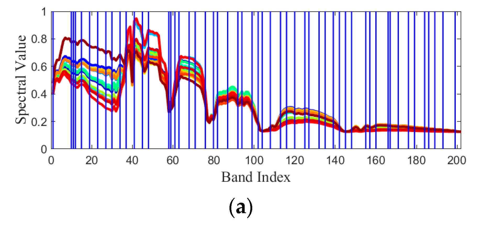
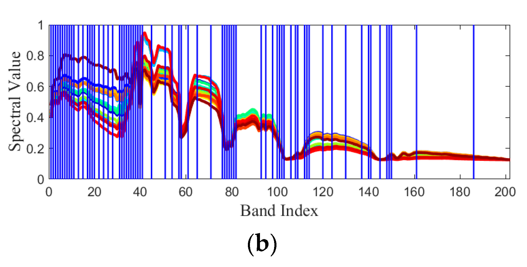
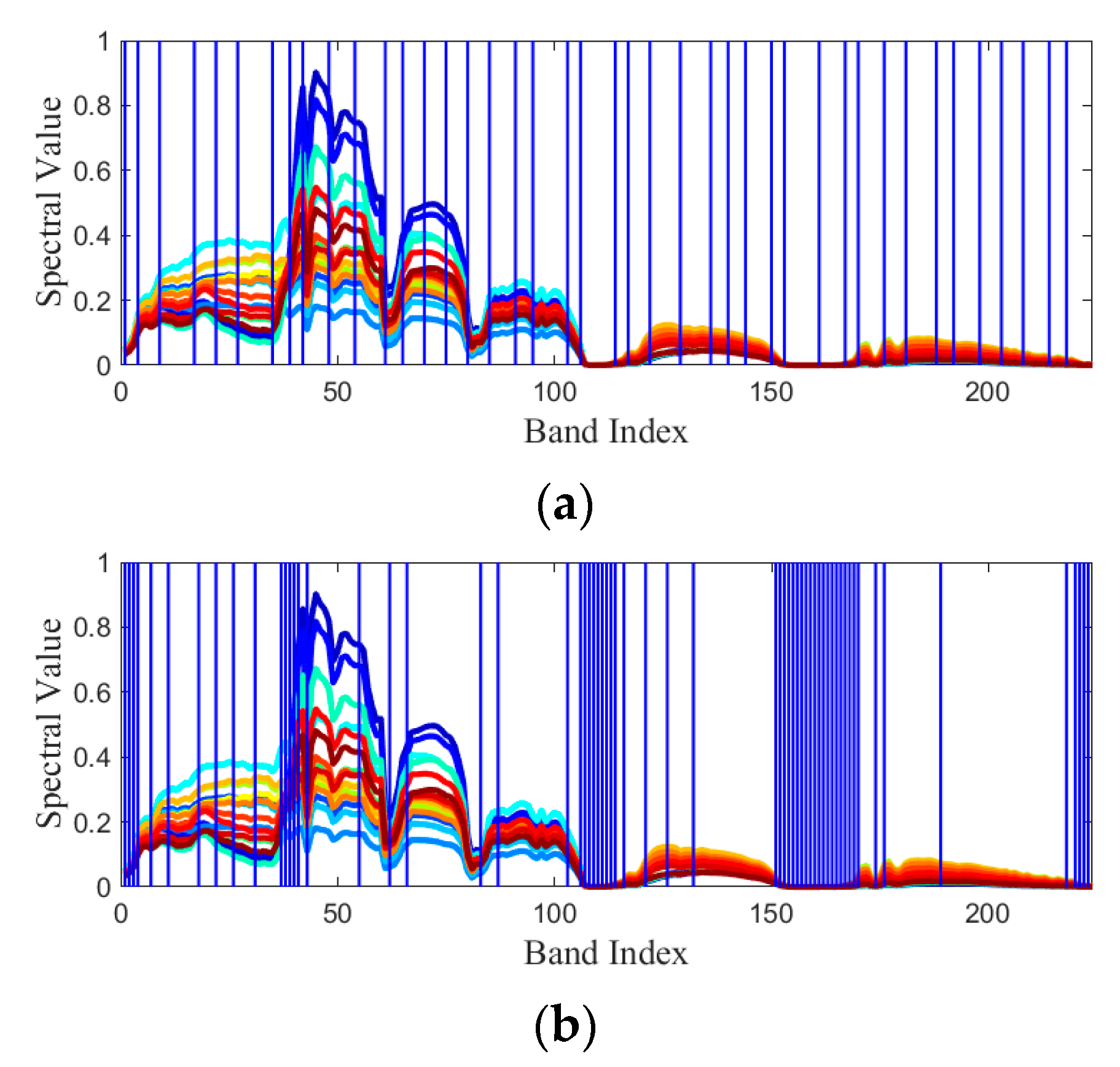
  • The results of CCBSS, PBS, and LCMV-BSS have two issues: selecting adjacent bands and selecting the bands in specific spectral regions. For example, in Table 3, bands 98–103 were selected by PBS, bands 50–57 and 88–96 were selected by SC CCBSS, and bands 1–5, 60–61, and 88–96 were selected by SQ LCMV-BSS. Similar phenomenon can also be found in Table 4 and Table 5.
  • The first issue was significantly alleviated in SC/SQ SSRBSS and OMP-BS. Their selected bands were distributed more uniformly in the whole spectrum. However, there are still cases where the bands in a certain range were ignored to be selected. For example, in Table 4, bands 125–188 were missing from the SC SSRBSS result, while bands 123–190 were missing from the SQ SSRBSS result. A similar phenomenon can also be found in Table 5.
  • The FNG-SSRBSS and BD-SSRBSS methods seemed to overcome both issues. Not only did they reduce the probability of selecting adjacent bands, but they ensured that each segment of the spectrum could generate at least one band for better information integrity.
  • The BG results of FNG-SSRBSS and BD-SSRBSS were obviously different. The group size of the band groups produced by FNG tended to be consistent, while the group size of the BD-generated band groups varied greatly. For instance, in the results for SQ BD-SSRBSS in Table 5, there are three band groups consisting of only 1 band: {3}, {41}, and {222}, and one group containing 29 bands: {190–218}. On the contrary, the group size produced by FNG consistently ranged from 2 to 6. This is due to the inherent nature of each BG algorithm.

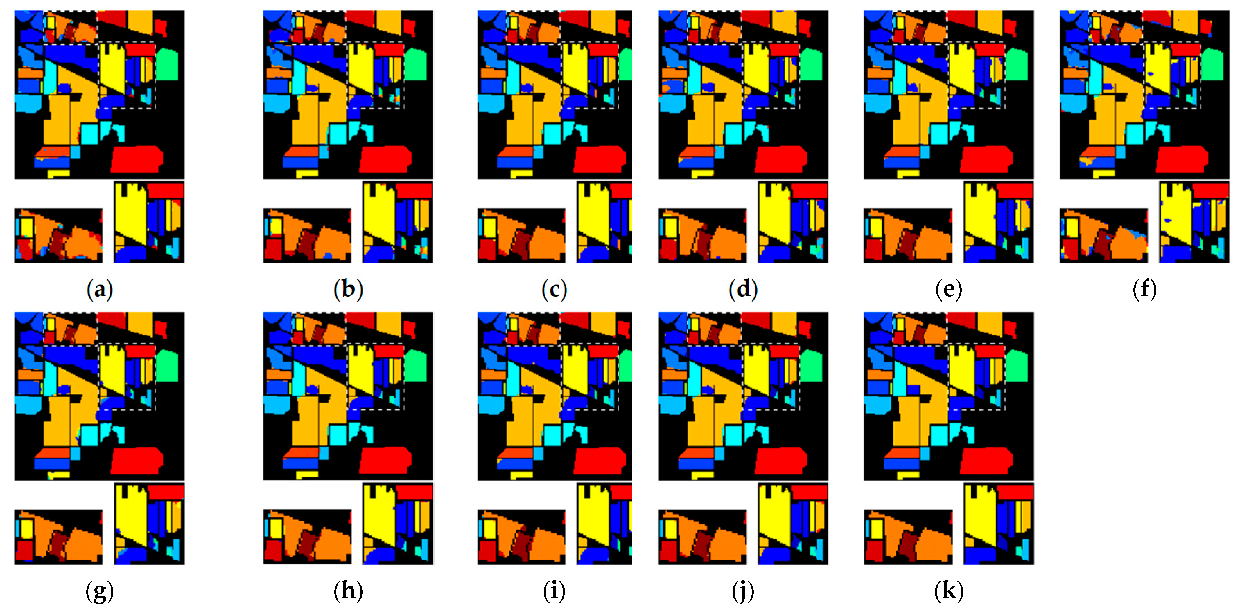
6.4. Classification Results

This section shows the HSI classification results of using two different classifiers performed on the selected bands of various BS methods.

6.4.1. SVM Results

In this section, we adopted the bands selected by UBS, OMP-BS, PBS, FNGBS, SQ CCBSS, SC LCMV-BSS, and the proposed six BG-SSRBSS methods for image classification on the three HSI datasets. Both quantitative and qualitative analysis is presented.
Table 6, Table 7 and Table 8 present the SVM classification results of using the bands listed in Table 3, Table 4, and Table 5, respectively, for Pavia, Purdue, and Salinas datasets. The bold values in each table represents the highest accuracies in the corresponding class. From Table 6, it can be observed that in addition to FNGBS, SQ CCBSS, and SC LCMV-BSS, which only produced 75.66% and 84.28% in OA, the other BS methods, UBS, OMP-BS, PBS, and SC/SQ SSRBSSs could produce 88–90% in OA. We speculate that this is due to their selected bands being more complementary in the spectrum. Among all BS methods, the proposed SQ BS-SSRBSS-2 produced the highest accuracies in OA, AA, and Kappa: 90.57%, 86.3%, and 87.17%. In general, the Pavia data are relatively simpler data for classification. Using the selected bands provided by most BS methods could provide satisfactory classification performance.
Compared to the Pavia dataset, the Purdue dataset is a heavily-mixed image and was considered much more difficult to be classified in the literature. The performance difference between various BS methods can be observed more through the experiments classifying Purdue data. From Table 7, it is found that the OA range is from 60% to 80%. The OA values generated by UBS, PBS, FNGBS, CQ CCBSS, and SC LCMV-BSS are 74.8%, 74.45%, 78.52%, 60.83%, and 62.82%, respectively. Using the bands selected by the proposed SC/SQ SSRBSS, SC/SQ FNG-SSRBSS, and SC/SQ BD-SSRBSS achieved 76–80% in OA. The highest OA, AA, and Kappa values were generated by SQ FNG-SSRBSS: 80.18%, 73.73%, and 77.4%. Additionally, most of the best single-class values were produced by our SSRBSS methods. Similar to Pavia’s classification results shown in Table 6, the performance of SQ CCBSS and SC LCMV-BSS was relatively lower in the comparison. It verifies that the bands selected by the proposed BG-SSRBSS methods contain a larger amount of spectral information to identify different substances.
Among three datasets, the Salinas dataset is the one relatively easier to be classified. From Table 8, it can be seen that except for class 8 and class 15, the accuracy values of the other 14 classes are as high as 98–99%. In addition to PBS and SQ CCBSS, which only provided 85.71% and 87.25% in OA, the other BS methods achieved 90–91% in OA. Similarly, the proposed SQ FNG-SSRBSS achieved the highest overall accuracy of 91.7%. At the same time, the proposed SSRBSS methods produced the best single-class accuracies in classes 1, 2, 4–8, and 10–17.
From the above-mentioned observations, it is concluded that the proposed BG-SSRBSS methods outperformed the compared BS methods. It is worth noting that using BG-SSRBSS’s selected bands could even produce a better classification performance than using full bands in the Purdue and Salinas experiments.

6.4.2. HybridSN Results

The classification performance via a spatial–spectral classifier for various BS methods is another focus of observation. Table 9, Table 10 and Table 11 present the HybridSN classification results of using the bands listed in Table 3, Table 4, and Table 5, respectively, for the Pavia, Purdue, and Salinas datasets. By virtue of the information integration capability through spatial and spectral dimensions of CNN, the classification performance on the Pavia and Salinas datasets was close to 100%. Simultaneously, the classification results of the Purdue data were also greatly improved to 98%. Almost all BS methods reached nearly the same classification performance as using full bands. Despite the powerful classification capabilities provided by HybridSN, the proposed SSRBSS methods still slightly outperform the other ones. It was found that the best OA in Table 11 was obtained by using SC FNG-SSRBSS (99.77%), the best OA in Table 10 was obtained by using SQ SSRBSS, and the best OA in Table 11 was obtained by SC BD-SSRBSS.
In order to see the difference in using various BS approaches by visual assessment, Figure 7 shows the HybridSN classification maps of the Pavia dataset by using full bands and the bands selected by various BS methods. Although those maps are similar, the advantages of BG-SSRBSS can be seen in tiny details. For instance, in the maps of UBS and SQ CCBSS, Figure 7b,e, several pixels in the prairie below the scene were misclassified as bare soil or trees instead of meadows. In the cropped image, a few pixels of gravel (cyan) were misclassified as self-blocking bricks (red) in the maps of SQ CCBSS and SC LCMV-BSS. These tiny classification defects were relatively absent from the results of the SQ SSRBSS and SC FNG-SSRBSS methods shown in Figure 7h,i. Similarly, Figure 8 shows the HybridSN classification maps of Purdue image by using full bands and the bands selected by various BS methods. There are several obvious classification flaws could be found in the maps of the compared BS methods, for example, classes 3, 12 in Figure 8a; classes 2, 4, 5 in Figure 8b; classes 3, 4, 11 in Figure 8d; classes 2, 3, 11, 14, in Figure 8e; and classes 2, 4, 11 in Figure 8f. In contrast, there are significantly fewer misclassification pixels in BG-SSRBSS’s maps shown in Figure 8g–i. Finally, Figure 9 shows the HybridSN classification maps of the Salinas dataset by using full bands and the bands selected by various BS methods. In the maps of the compared BS methods (Figure 9b–f), it can be observed that a few pixels located in class 8 (Grape-untrained) and class 15 (Vineyard-untrained) were misclassified. Surprisingly, such an issue is milder in the proposed BG-SSRBSS’s maps shown in Figure 9g–i. In conclusion, the result of visual assessment also verifies the strength of the proposed BG-SSRBSS.

6.5. Discussion

In addition to the quantitative analysis and visual comparison presented in Section 6.4, there are additional findings from Table 3, Table 4, Table 5, Table 6, Table 7, Table 8, Table 9, Table 10 and Table 11 worthy of mentioning:
  • According to Table 3, Table 4, Table 5, Table 6, Table 7 and Table 8, the BS methods that utilize sparse self-representation as objective function, OMP-BS and SSRBSSs, significantly outperformed the other ones. It implies that the SSR model is indeed an ideal objective function for BS in hyperspectral image classification.
  • According to Table 3, Table 4, Table 5, Table 6, Table 7 and Table 8, the BS methods that utilize sparse self-representation as objective function, OMP-BS and SSRBSSs, significantly outperformed the other ones. It implies that the SSR model is indeed an ideal objective function for BS in hyperspectral image classification.
  • The classification performance of using full bands was usually not the best. This shows that the excessive redundant information in full bands could interfere with the performance of the classifier due to the curse of dimensionality.
  • Among all BSS methods, the proposed BG-SSRBSSs significantly outperformed SQ CCBSS and SC LCMV-BSS, particularly in Purdue’s experiment. This implies that SSR is a more suitable objective function than CC or LCMV for selecting the bands useful for classification.
  • According to the results of six BG-SSRBSSs, the classification accuracy of using SC and SQ search methods are quite similar, even though their final selected band groups are slightly different. This suggests that both of them could find good local optimal solutions.
As we know, the BG plays an important role for BG-SSRBSS. Here we further investigate the NBG performance of two BG methods. Figure 10, Figure 11 and Figure 12 demonstrate the FNG and BD results of the Pavia, Purdue, and Salinas datasets, respectively. In each figure, the x-axis denotes band index, the y-axis denotes spectral reflectance, and the vertical blue line indicates the boundary of two adjacent band groups. Each spectral curve represents the spectral signature of the class with the same color in the corresponding ground truth map shown in Figure 4, Figure 5 and Figure 6. As we can see, the BG results of using FNG and BD are quite different. The FNG seems to segment the spectrum more uniformly, while the BD tends to segment more in the regions whose spectral values of different classes are lower or closed. However, after the selection done by BGSS, the resulting bands made no obvious difference in classification performance. This shows that the given g values are large enough so that all BG-SSRBSSs could find the ideal band group combinations for effective classification.
Since BG-SSRBSS belongs to a search-based BS method, its computation speed is worthy of attention. Table 12 tabulates the computing times in seconds for OMP-BS, PBS, SC/SQ CCBSS (SAM), SC/SQ LCMV-BSS, and the proposed six BG-SSRBSS methods.
The computing time of each BG-SSRBSS method is expressed as the summation of the time required by BG and BGSS. It is apparent that the proposed BG-SSRBSS (FNG-SSRBSS and BD-SSRBSS) require less time than CCBSS and LCMV-BSS in most cases, particularly for the Purdue and Salinas datasets. Another interesting point is that the FNG-SSRBSS and BD-SSRBSS require less computing time than the SSRBSS. This is simply because the number of iterations required for SC/SQ searches was drastically reduced. More specifically, the SSRBSS roughly requires a total of ( L p )   ×   p computations of the optimizations of the SSR model, while the BGSSRBS only requires a total of (g p) × p computations. Although the size of the matrix P formed in BG-SSRBSS is larger than that in SSRBSS, the overall computation time did not increase dramatically because the optimization of the SSR model could be efficiently calculated with Matlab. Overall, compared with the existing BSS methods, the proposed BG-SSRBSS can strike a balance between classification accuracy and computational complexity.

7. Conclusions

This paper developed a new BS method, called BG-SSRBSS, which can select an informative band subset for hyperspectral image classification. The BG-SSRBSS consists of two parts: band grouping (BG) and band group subset selection (BGSS). The BG divides entire bands into several non-overlapping band groups in the direction of the spectrum. It can be viewed as a pre-decorrelation process. Using BG not only reduces the similarity between selected bands, but also decreases the number of iterations required in BGSS’s search so as to reduce computing time. The BGSS aims to find the optimal band group subset with minimal reconstruction error of the SSR model via SC or SQ search. Finally, the representative bands of the optimal band group subset are taken as the BS result. The experiments conducted on three HSI datasets show that using the bands selected by BG-SRBSSS could achieve better classification accuracy than state-of-the-art methods either with two different classifiers.
It is worth noted that if BG is not used, the BG-SSRBSS will degenerate to a typical BSS approach, called SSRBSS. From this point of view, the proposed BG-SSRBSS enlarges the existing BSS framework to a brand new approach: Band-grouping-based BSS (BG-BSS). How to produce better band groups as the input of BG-BSS would be an interesting topic. On the other hand, the current BSS approaches, as well as our BG-SSRBSS, can be run with multiple cycles. That is, it is able to use the result of the first run as the input of the next run. Doing so may prompt BSS to find better band subsets. This part will be reserved for our future work. Furthermore, there are several points that can be improved under the existing BSS framework. For instance, how to select a more appropriate initial band subset to reach the global optima, and how to provide a guidance that can automatically determine the value of parameter g in BG-BSS. Those parts will also be investigated in the future.

Author Contributions

Conceptualization, K.-H.L.; methodology, K.-H.L.; software and data curation, Y.-K.C. and T.-Y.C.; writing—original draft preparation, K.-H.L.; writing—review and editing, K.-H.L. and Y.-K.C. All authors have read and agreed to the published version of the manuscript.

Funding

This research was supported in part by the National Science and Technology Council (NSTC) in Grant No.: NSTC 111-2221-E-110-030-MY2.

Data Availability Statement

Publicly available datasets were analyzed in this study. This data can be found here: https://www.ehu.eus/ccwintco/index.php/Hyperspectral_Remote_Sensing_Scenes.

Conflicts of Interest

The authors declare no conflict of interest.

References

  1. Sun, W.; Du, Q. Hyperspectral Band Selection: A Review. IEEE Geosci. Remote Sens. Mag. 2019, 7, 118–139. [Google Scholar] [CrossRef]
  2. Patro, R.N.; Subudhi, S.; Biswal, P.K.; Dell’Acqua, F. A Review of Unsupervised Band Selection Techniques: Land Cover Classification for Hyperspectral Earth Observation Data. IEEE Geosci. Remote Sens. Mag. 2021, 9, 72–111. [Google Scholar] [CrossRef]
  3. Chang, C.-I.; Du, Q.; Sun, T.-L.; Althouse, M.L. A joint band prioritization and band-decorrelation approach to band selection for hyperspectral image classification. IEEE Trans. Geosci. Remote Sens. 1999, 37, 2631–2641. [Google Scholar] [CrossRef] [Green Version]
  4. Chang, C.-I.; Wang, S. Constrained band selection for hyperspectral imagery. IEEE Trans. Geosci. Remote Sens. 2006, 44, 1575–1585. [Google Scholar] [CrossRef]
  5. Huang, R.; He, M. Band selection based on feature weighting for classification of hyperspectral data. IEEE Geosci. Remote Sens. Lett. 2005, 2, 156–159. [Google Scholar] [CrossRef]
  6. Chang, C.-I.; Liu, K.-H. Progressive Band Selection of Spectral Unmixing for Hyperspectral Imagery. IEEE Trans. Geosci. Remote Sens. 2014, 52, 2002–2017. [Google Scholar] [CrossRef]
  7. Du, Q.; Yang, H. Similarity-based unsupervised band selection for Hyperspectral Image Analysis. IEEE Geosci. Remote Sens. Lett. 2008, 5, 564–568. [Google Scholar] [CrossRef]
  8. Yin, J.; Wang, Y.; Hu, J. A New Dimensionality Reduction Algorithm for Hyperspectral Image Using Evolutionary Strategy, IEEE Trans. Ind. Informat. 2012, 8, 935–943. [Google Scholar] [CrossRef]
  9. Feng, J.; Jiao, L.; Zhang, X.; Sun, T. Hyperspectral band selection based on trivariate mutual information and clonal selection. IEEE Trans. Geosci. Remote Sens. 2014, 52, 4092–4105. [Google Scholar] [CrossRef]
  10. Su, H.; Du, Q.; Chen, G.; Du, P. Optimized Hyperspectral Band Selection Using Particle Swarm Optimization. IEEE J. Sel. Topics Appl. Earth Observ. Remote Sens. 2014, 7, 2659–2670. [Google Scholar] [CrossRef]
  11. Ghamisi, P.; Couceiro, M.S.; Benediktsson, J.A. A Novel Feature Selection Approach Based on FODPSO and SVM. IEEE Trans. Geosci. Remote Sens. 2015, 53, 2935–2947. [Google Scholar] [CrossRef] [Green Version]
  12. Su, H.; Yong, B.; Du, Q. Hyperspectral Band Selection Using Improved Firefly Algorithm. IEEE Geosci. Remote Sens. Lett. 2016, 13, 68–72. [Google Scholar] [CrossRef]
  13. Medjahed, S.A.; Ait Saadi, T.; Benyettou, A.; Ouali, M. Gray Wolf Optimizer for Hyperspectral Band Selection. Appl. Soft Comput. 2016, 40, 178–186. [Google Scholar] [CrossRef]
  14. Imbiriba, T.; Bermudez, J.C.M.; Richard, C. Band Selection for Nonlinear Unmixing of Hyperspectral Images as a Maximal Clique Problem. IEEE Trans. Image Process. 2017, 26, 2179–2191. [Google Scholar] [CrossRef] [Green Version]
  15. Wang, C.; Gong, M.; Zhang, M.; Chan, Y. Unsupervised Hyperspectral Image Band Selection via Column Subset Selection. IEEE Geosci. Remote Sens. Lett. 2015, 12, 1411–1415. [Google Scholar] [CrossRef]
  16. Wang, L.; Li, H.; Xue, B.; Chang, C. Constrained Band Subset Selection for Hyperspectral Imagery. IEEE Geosci. Remote Sens. Lett. 2017, 14, 2032–2036. [Google Scholar] [CrossRef]
  17. Chang, C.; Lee, L.; Xue, B.; Song, M.; Chen, J. Channel Capacity Approach to Hyperspectral Band Subset Selection. IEEE J. Sel. Topics Appl. Earth Observ. Remote Sens. 2017, 10, 4630–4644. [Google Scholar] [CrossRef]
  18. Yu, C.; Song, M.; Chang, C.-I. Band Subset Selection for Hyperspectral Image Classification. Remote Sens. 2018, 10, 113. [Google Scholar] [CrossRef] [Green Version]
  19. Yuan, Y.; Lin, J.; Wang, Q. Dual-clustering-based hyperspectral band selection by contextual analysis. IEEE Trans. Geosci. Remote Sens. 2016, 54, 1431–1445. [Google Scholar] [CrossRef]
  20. Zhu, G.; Huang, Y.; Lei, J.; Bi, Z.; Xu, F. Unsupervised hyperspectral band selection by dominant set extraction. IEEE Trans. Geosci. Remote Sens. 2016, 54, 227–239. [Google Scholar] [CrossRef]
  21. Yang, C.; Tan, Y.; Bruzzone, L.; Lu, L.; Guan, R. Discriminative feature metric learning in the affinity propagation model for band selection in hyperspectral images. Remote Sens. 2017, 9, 782. [Google Scholar] [CrossRef] [Green Version]
  22. Yuan, Y.; Zheng, X.; Lu, X. Discovering Diverse Subset for Unsupervised Hyperspectral Band Selection. IEEE Trans. Image Process. 2017, 26, 51–64. [Google Scholar] [CrossRef] [PubMed]
  23. Zeng, M.; Cai, Y.; Cai, Z.; Liu, X.; Hu, P.; Ku, J. Unsupervised Hyperspectral Image Band Selection Based on Deep Subspace Clustering. IEEE Geosci. Remote Sens. Lett. 2019, 16, 1889–1893. [Google Scholar] [CrossRef]
  24. Li, S.; Qi, H. Sparse representation based band selection for hyperspectral images. In Proceedings of the 18th IEEE International Conference on Image Processing, Brussels, Belgium, 11–14 September 2011; IEEE: Piscataway, NJ, USA, 2011; pp. 2693–2696. [Google Scholar] [CrossRef]
  25. Li, H.; Wang, Y.; Duan, J.; Xiang, S.; Pan, C. Group sparsitybased semi-supervised band selection for hyperspectral images. In Proceedings of the IEEE International Conference on Image Processing, Melbourne, Australia, 15–18 September 2013; IEEE: Piscataway, NJ, USA; pp. 3225–3229. [Google Scholar] [CrossRef]
  26. Sun, W.; Zhang, L.; Du, B.; Li, W.; Mark Lai, Y. Band Selection Using Improved Sparse Subspace Clustering for Hyperspectral Imagery Classification. IEEE J. Sel. Topics Appl. Earth Observ. Remote Sens. 2015, 8, 2784–2797. [Google Scholar] [CrossRef]
  27. Lai, C.-H.; Chen, C.-S.; Chen, S.-Y.; Liu, K.-H. Sequential band selection method based on group orthogonal matching pursuit. In Proceedings of the 8th Workshop on Hyperspectral Image and Signal Processing: Evolution in Remote Sensing (WHISPERS), Los Angeles, CA, USA, 21–24 August 2016; pp. 1–4. [Google Scholar] [CrossRef]
  28. Sun, W.; Zhang, L.; Zhang, L.; Lai, Y.M. A Dissimilarity-Weighted Sparse Self-Representation Method for Band Selection in Hyperspectral Imagery Classification. IEEE J. Sel. Top. Appl. Earth Obs. Remote Sens. 2016, 9, 4374–4388. [Google Scholar] [CrossRef]
  29. Sun, W.; Tian, L.; Xu, Y.; Zhang, D.; Du, Q. Fast and Robust Self-Representation Method for Hyperspectral Band Selection. IEEE J. Sel. Top. Appl. Earth Obs. Remote Sens. 2017, 10, 5087–5098. [Google Scholar] [CrossRef]
  30. Kuo, B.-C.; Ho, H.-H.; Li, C.-H.; Hung, C.-C.; Taur, J.-S. A kernel-based feature selection method for SVM with RBF kernel for hyperspectral image classification. IEEE J. Select. Topics Appl. Earth Observ. Remote Sens. 2014, 7, 317–326. [Google Scholar] [CrossRef]
  31. Ribalta Lorenzo, P.; Tulczyjew, L.; Marcinkiewicz, M.; Nalepa, J. Hyperspectral Band Selection Using Attention-Based Convolutional Neural Networks. IEEE Access 2020, 8, 42384–42403. [Google Scholar] [CrossRef]
  32. Cai, R.; Yuan, Y.; Lu, X. Hyperspectral band selection with convolutional neural network. In Proceedings of the Chinese Conference on Pattern Recognition and Computer Vision (PRCV), Guangzhou, China, 23–26 November 2018; pp. 396–408. [Google Scholar] [CrossRef]
  33. Cai, Y.; Liu, X.; Cai, Z. BS-Nets: An end-to-end framework for band selection of hyperspectral image. IEEE Trans. Geosci. Remote Sens. 2020, 58, 1969–1984. [Google Scholar] [CrossRef] [Green Version]
  34. Feng, J.; Li, D.; Gu, J.; Cao, X.; Shang, R.; Zhang, X.; Jiao, L. Deep reinforcement learning for semisupervised hyperspectral band selection. IEEE Trans. Geosci. Remote Sens. 2022, 60, 5501719. [Google Scholar] [CrossRef]
  35. Chang, Y.-L.; Liu, J.-N.; Chen, Y.-L.; Chang, W.-Y.; Hsieh, T.-J.; Huang, B. Hyperspectral band selection based on parallelparticle swarm optimization and impurity function band prioritization schemes. J. Appl. Remote Sens. 2014, 8, 084798. [Google Scholar] [CrossRef]
  36. Paul, A.; Bhattacharya, S.; Dutta, D.; Sharma, J.R.; Dadhwal, V.K. Band selection in hyperspectral imagery using spatial cluster mean and genetic algorithms. GISci. Remote Sens. 2015, 52, 643–659. [Google Scholar] [CrossRef]
  37. Wang, Q.; Lin, J.; Yuan, Y. Salient band selection for hyperspectral image classification via manifold ranking. IEEE Trans. Neural Netw. Learn. Syst. 2016, 27, 1279–1289. [Google Scholar] [CrossRef]
  38. Xiong, W.; Chang, C.-I.; Wu, C.-C.; Kalpakis, K.; Chen, H.M. Fast Algorithms to Implement N-FINDR for Hyperspectral Endmember Extraction. IEEE J. Sel. Top. Appl. Earth Obs. Remote Sens. 2011, 4, 545–564. [Google Scholar] [CrossRef]
  39. Chang, C.-I. Real Time Progressive Hyperspectral Image Processing: Endmember Finding and Anomaly Detection; Springer: New York, NY, USA, 2016. [Google Scholar] [CrossRef]
  40. Chang, C.-I. Hyperspectral Imaging: Techniques for Spectral Detection and Classification; Springer Science & Business Media: Berlin/Heidelberg, Germany, 2003. [Google Scholar] [CrossRef]
  41. Chang, C.-I.; Du, Q. Estimation of number of spectrally distinct signal sources in hyperspectral imagery. IEEE Trans. Geosci. Remote Sens. 2004, 42, 608–619. [Google Scholar] [CrossRef] [Green Version]
  42. Yu, H.; Gao, L.; Liao, W.; Zhang, B. Group Sparse Representation Based on Nonlocal Spatial and Local Spectral Similarity for Hyperspectral Imagery Classification. Remote Sens. 2018, 18, 1695. [Google Scholar] [CrossRef] [Green Version]
  43. Sun, W.; Jiang, M.; Li, W.; Liu, Y. A Symmetric Sparse Representation Based Band Selection Method for Hyperspectral Imagery Classification. Remote Sens. 2016, 8, 238. [Google Scholar] [CrossRef] [Green Version]
  44. Iordache, M.-D.; Bioucas-Dias, J.M.; Plaza, A. Collaborative Sparse Regression for Hyperspectral Unmixing. IEEE Trans. Geosci. Remote Sens. 2014, 52, 341–354. [Google Scholar] [CrossRef] [Green Version]
  45. Li, C.; Ma, Y.; Mei, X.; Liu, C.; Ma, J. Hyperspectral Unmixing with Robust Collaborative Sparse Regression. Remote Sens. 2016, 8, 588. [Google Scholar] [CrossRef] [Green Version]
  46. Elhamifar, E.; Sapiro, G.; Vidal, R. See all by looking at a few: Sparse modeling for finding representative objects. In Proceedings of the IEEE Conference on Computer Vision and Pattern Recognition, Providence, RI, USA, 16–21 June 2012; IEEE: Piscataway, NJ, USA, 2012; pp. 1600–1607. [Google Scholar] [CrossRef] [Green Version]
  47. Wang, Q.; Li, Q.; Li, X. A Fast Neighborhood Grouping Method for Hyperspectral Band Selection. IEEE Trans. Geosci. Remote Sens. 2021, 59, 5028–5039. [Google Scholar] [CrossRef]
  48. Lozano, A.C.; Świrszcz, G.; Abe, N. Group Orthogonal Matching Pursuit for variable selection and prediction. In Proceedings of the 22nd International Conference on Neural Information Processing Systems, Red Hook, NY, USA, 6–14 December 2009; pp. 1150–1158. [Google Scholar]
  49. Chang, C.-I. Hyperspectral Data Processing: Algorithm Design and Analysis; John Wiley & Sons: Hoboken, NJ, USA, 2013. [Google Scholar] [CrossRef]
  50. Bigdeli, B.; Samadzadegan, F.; Reinartz, P. Band Grouping versus Band Clustering in SVM Ensemble Classification of Hyperspectral Imagery. Photogramm. Eng. Remote Sens. 2013, 79, 523–533. [Google Scholar] [CrossRef]
  51. Hyperspectral Remote Sensing Scenes. Available online: https://www.ehu.eus/ccwintco/index.php/Hyperspectral_Remote_Sensing_Scenes (accessed on 6 October 2022).
  52. Chang, C.-C.; Lin, C.-J. LIBSVM: A library for support vector machines. ACM Trans. Intell. Syst. Technol. 2011, 2, 1–27. [Google Scholar] [CrossRef]
  53. Roy, S.K.; Krishna, G.; Dubey, S.R.; Chaudhuri, B.B. HybridSN: Exploring 3-D–2-D CNN Feature Hierarchy for Hyperspectral Image Classification. IEEE Geosci. Remote Sens. Lett. 2020, 17, 277–281. [Google Scholar] [CrossRef]
Figure 1. The concept of SSR model for BS.
Remotesensing 14 05686 g001
Figure 2. The mechanism of BG-SSRBSS.
Remotesensing 14 05686 g002
Figure 3. The block diagram of BG-SSRBSS.
Remotesensing 14 05686 g003
Figure 4. Pavia image scene. (a) Band 80th; (b) Ground truth map for nine classes; (c) Ground truth class label.
Remotesensing 14 05686 g004
Figure 5. Purdue image scene. (a) Band 20th; (b) Ground truth map; (c) Ground truth class labels.
Remotesensing 14 05686 g005
Figure 6. Salinas image scene. (a) Band 170th; (b) Ground truth map; (c) Ground truth class labels.
Remotesensing 14 05686 g006
Figure 7. Classification maps generated by HybridSN using different BS methods for the Pavia dataset: (a) Full bands; (b) UBS; (c) OMP-BS; (d) PBS; (e) FNGBS; (f) SQ CCBSS; (g) LCMV-BSS; (h) SQ SSRBSS; (i) SC FNG-SSRBSS; (j) SQ BD-SSRBSS; (k) Ground truth.
Remotesensing 14 05686 g007
Figure 8. Classification maps generated by HybridSN using different BS methods for the Purdue dataset: (a) Full bands; (b) UBS; (c) OMP-BS; (d) PBS; (e) FNGBS; (f) SQ CCBSS; (g) LCMV-BSS; (h) SQ SSRBSS; (i) SQ FNG-SSRBSS; (j) SC BD-SSRBSS; (k) Ground truth.
Remotesensing 14 05686 g008
Figure 9. Classification maps generated by HybridSN using different BS methods for the Salinas dataset: (a) Full bands; (b) UBS; (c) OMP-BS; (d) PBS; (e) FNGBS; (f) SQ CCBSS; (g) LCMV-BSS; (h) SC SSRBSS; (i) SQ FNG-SSRBSS; (j) SQ BD-SSRBSS; (k) Ground truth.
Remotesensing 14 05686 g009
Figure 10. The BG results for the Pavia experiment. (a) FNG; (b) BD.
Remotesensing 14 05686 g010
Figure 11. The BG results for the Purdue experiment. (a) FNG; (b) BD.
Remotesensing 14 05686 g011aRemotesensing 14 05686 g011b
Figure 12. The BG results for the Salinas experiment. (a) FNG; (b) BD.
Remotesensing 14 05686 g012
Table 1. The names and definition of six BG-SSRBSS methods.
Method’s NameBG MethodSearch Method for BGSSRelationship of g, p, and L
SC FNG-SSRBSSFNGSC p     g   <   L
(w/BG)
SC BD-SSRBSSBD
SQ FNG-SSRBSSFNGSQ
SQ BD-SSRBSSBD
SC SSRBSSn/aSC p   <   g = L
(w/o BG)
SQ SSRBSSn/aSQ
Table 2. The parameters of BG-SSRBSS used in the experiment.
Pg (FNG) g (BD)
Pavia data175168
Purdue data185472
Salinas data214263
Table 3. The bands selected by the proposed and the compared methods for the Pavia dataset.
DataMethodSelected Bands
Pavia
(16 bands)
UBS1, 7, 13, 19, 25, 31, 37, 43, 49, 55, 61, 67, 73, 79, 85, 91, 103
OMP-BS [27]1, 2, 4, 6, 9, 13, 24, 33, 42, 54, 66, 74, 81, 83, 86, 94, 100
PBS [6]1, 27, 37, 43, 51, 52, 64, 83, 89, 91, 94, 95, 98, 100, 101, 102, 103
FNGBS [47]5, 12, 19, 22, 30, 32, 42, 49, 56, 61, 63, 74, 79, 81, 88, 92, 99
SC CCBSS [17]50, 51, 52, 53, 54, 55, 56, 57, 88, 89, 90, 91, 92, 93, 94, 95, 96
SQ CCBSS [17]15, 16, 17, 18, 19, 20, 21, 87, 88, 89, 90, 91, 92, 93, 94, 95, 96
SC LCMV-BSS [18]1, 2, 3, 4, 5, 6, 48, 55, 68, 69, 81, 87, 89, 91, 98, 100, 103
SQ LCMV-BSS [18]1, 2, 3, 4, 5, 59, 60, 61, 88, 89, 90, 91, 92, 93, 94, 95, 96
SC SSRBSS1, 2, 4, 5, 7, 10, 13, 24, 33, 44, 54, 64, 71, 81, 85, 97, 102
SQ SSRBSS1, 2, 3, 5, 8, 12, 20, 31, 44, 54, 64, 73, 82, 83, 85, 94, 101
SC FNG-SSRBSS2{1–3}, 4{4,5}, 6{6,7}, 10{10,11}, 15{14–17}, 22{22,23}, 29{28–30}, 39{38–40}, 48{48,49}, 54{54,55}, 62{62,63}, 72{72,73}, 76{76,77}, 83{82–84}, 89{88–90}, 97{97,98}, 102{102,103}
SQ FNG-SSRBSS2{1–3}, 4{4,5}, 6{6,7}, 8{8,9}, 15{14–17}, 31{31}, 44{44,45}, 54{54,55}, 60{60,61}, 68{68,69}, 74{74,75}, 83{82–84}, 85{85}, 86{86,87}, 95{94–96}, 99{99}, 102{102,103}
SC BD-SSRBSS1{1,2}, 4{4}, 6{6}, 9{9}, 13{13}, 19{19,20}, 31{31,32}, 43{43,44}, 47{47,48}, 55{55,56}, 66{66}, 73{73}, 79{79}, 82{82,83}, 85{85}, 94{92–96}, 101{100–102}
SQ BD-SSRBSS1{1,2}, 4{4}, 6{6}, 8{8}, 11{11}, 19{19,20}, 31{31,32}, 41{41,42}, 53{53,54}, 66{66}, 74{74}, 80{80,81}, 82{82,83}, 85{85}, 94{92–96}, 101{100–102}, 103{103}
Table 4. The bands selected by the proposed and the compared methods for the Purdue dataset.
DataMethodSelected Bands
Purdue
(17 bands)
UBS1, 13, 25, 37, 49, 61, 73, 85, 97, 109, 121, 133, 145, 157, 169, 181, 193, 202
OMP-BS [27]1, 2, 3, 4, 6, 9, 19, 29, 34, 38, 42, 50, 68, 81, 97, 113, 131, 189
PBS [6]1, 7, 10, 26, 34, 44, 46, 48, 57, 65, 66, 85, 87, 92, 107, 157, 166, 196
FNGBS [47]9, 15, 28, 43, 49, 59, 66, 83, 97, 107, 118, 129, 138, 157, 165, 173, 181, 190
SC CCBSS [17]45, 46, 47, 48, 49, 50, 51, 52, 53, 155, 156, 160, 161, 162, 163, 164, 165, 166
SQ CCBSS [17]10, 11, 12, 13, 14, 15, 16, 17, 44, 45, 46, 47, 48, 49, 50, 51, 52, 53
SC LCMV-BSS [18]3, 6, 11, 24, 41, 70, 103, 143, 144, 145, 166, 190, 192, 193, 194, 195, 198, 200
SQ LCMV-BSS [18]13, 63, 65, 66, 69, 70, 72, 75, 89, 103, 119, 123, 168, 169, 171, 195, 197, 198
SC SSRBSS1, 2, 3, 4, 12, 15, 25, 32, 34, 37, 41, 42, 52, 68, 90, 98, 124, 189
SQ SSRBSS1, 2, 3, 4, 7, 8, 18, 30, 33, 35, 38, 42, 53, 62, 72, 90, 122, 191
SC FNG-SSRBSS5{1–10}, 14{13–15}, 18{16–19}, 21{20–23}, 26{24–27}, 33{31–34}, 36{35–37}, 39{38–41}, 44{42–45}, 47{46–48}, 54{49,58}, 65{64–68}, 74{72–76}, 86{83–87}, 88{88–92}, 95{95–99}, 123{121–125}, 154{149–155}
SQ FNG-SSRBSS5{1–10}, 14{13–15}, 26{24–27}, 33{31–34}, 36{35–37}, 39{38–41}, 44{42–45}, 47{46–48}, 62{62–63}, 74{72–76}, 93{93,94}, 119{117–120}, 123{121–125}, 126{126,127}, 147{146–148}, 156{156,157}, 159{158–160}, 192{190–193}
SC BD-SSRBSS1{1,2}, 3{3}, 4{4}, 5{5}, 9{9}, 12{12,13}, 16{16,17}, 27{27,28}, 32{32}, 35{35}, 38{38}, 44{42–45}, 51{46–51}, 69{66–71}, 85{83–93}, 97{96–98}, 123{121–124}, 193{187–202}
SQ BD-SSRBSS1{1,2}, 3{3}, 4{4}, 5{5}, 12{12,13}, 16{16,17}, 27{27,28}, 33{33}, 35{35}, 38{38}, 44{42–45}, 53{52–54}, 74{72–76}, 85{83–93}, 97{96–98}, 123{121–124}, 149{149}, 193{187–202}
Table 5. The bands selected by the proposed and the compared methods for the Salinas dataset.
DataMethodSelected Bands
Salinas
(21 bands)
UBS1, 12, 23, 34, 45, 56, 67, 78, 89, 100, 111, 122, 133, 144, 155, 166, 177, 188, 199, 210, 224
OMP-BS [27]1, 2, 3, 4, 8, 14, 19, 23, 31, 34, 37, 39, 42, 50, 66, 72, 104, 121, 126, 152, 198
PBS [6]1, 20, 60, 197, 203, 204, 207, 208, 209, 210, 211, 213, 214, 215, 216, 217, 219, 221, 222, 223, 224
FNGBS [47]7, 15, 31, 38, 55, 62, 67, 83, 92, 96, 118, 122, 137, 147, 152, 166, 172, 187, 196, 212, 217
SC CCBSS [17]1, 2, 3, 4, 5, 10, 18, 26, 34, 37, 39, 42, 48, 57, 70, 76, 85, 134, 152, 170, 184
SQ CCBSS [17]26, 27, 28, 29, 30, 31, 32, 33, 34, 35, 42, 43, 44, 45, 46, 47, 48, 49, 50, 51, 52
SC LCMV-BSS [18]27, 44, 54, 61, 64, 74, 80, 88, 94, 104, 124, 134, 144, 154, 164, 174, 184, 194, 204, 214, 216
SQ LCMV-BSS [18]1, 2, 6, 24, 27, 28, 34, 44, 46, 54, 74, 84, 104, 114, 134, 144, 164, 174, 184, 194, 204
SC SSRBSS1, 2, 3, 4, 5, 10, 18, 26, 34, 37, 39, 42, 48, 57, 70, 76, 85, 134, 152, 170, 184
SQ SSRBSS1, 2, 3, 4, 5, 9, 14, 20, 28, 35, 38, 41, 46, 55, 67, 76, 83, 92, 134, 170, 184
SC FNG-SSRBSS3{1–4}, 6{5–9}, 12{10–17}, 21{18–22}, 33{28–35}, 37{36–39}, 41{40–42}, 47{43–48}, 58{55–61}, 68{66–70}, 78{76–80}, 94{92–95}, 133{130–136}, 142{141–144}, 152{151–153}, 165{162–167}, 175{171–176}, 185{182–188}, 193{193–198}, 201{199–203}, 215{215–218}
SQ FNG-SSRBSS3{1–4}, 6{5–9}, 12{10–17}, 21{18–22}, 33{28–35}, 37{36–39}, 41{40–42}, 47{43–48}, 53{49–54}, 58{55–61}, 68{66–70}, 78{76–80}, 94{92–95}, 133{130–136}, 152{151–153}, 169{168–170}, 175{171–176}, 178{177–181}, 185{182–188}, 193{193–198}, 215{215–218}
SC BD-SSRBSS1{1,2}, 3{3}, 4{4}, 7{5–7}, 9{8–11}, 21{19–22}, 33{32–37}, 40{40}, 51{44–55}, 75{67–83}, 89{88–103}, 115{115,116}, 130{127–132}, 152{152}, 162{162}, 165{165}, 168{168}, 170{170}, 173{171–174}, 203{190–218}, 222{222}
SQ BD-SSRBSS1{1,2}, 3{3}, 4{4}, 7{5–7}, 15{12–18}, 21{19–22}, 29{27–31}, 33{32–37}, 38{38}, 41{41}, 51{44–55}, 60{56–62}, 75{67–83}, 89{88–103}, 130{127–132}, 152{152}, 162{162}, 165{165}, 173{171–174}, 203{190–218}, 222{222}
Table 6. SVM classification results of using the bands described in Table 3 for the Pavia dataset.
ClassFull Bands (Ref)UBSOMP-BSPBSFNGBSSQ CCBSSSC LCMV-BSSSC/SQ SSRBSSSC/SQ FNG-SSRBSSSQ BD-SSRBSS
191.1188.0585.7981.6685.774.9575.7384.18/85.3887.18/87.8287.99/87.24
294.4590.3591.7488.9985.970.6686.0691.53/90.8590.64/87.7992.1/92.1
388.7584.0885.5184.1884.1876.5668.6985.27/85.0884.8/85.5183.99/84.65
497.3596.597.0697.0696.0592.9595.9896.6/96.696.54/96.0896.21/96.89
599.9299.9299.9299.9299.8599.799.9299.92/99.299.92/99.9299.92/99.92
694.8192.590.6987.278879.2687.6792.1/91.890.69/89.8391.01/90.89
795.1893.9894.1394.1394.6693.392.6393.45/93.993.75/94.5194.73/93.98
889.0884.2785.0683.8184.4374.3379.7984.51/86.0485.14/84.7684.54/85.63
999.8999.8910010099.8910099.8999.89/10099.89/99.89100/100
OA93.3689.9890.3187.8686.7675.6684.2889.95/89.9589.68/88.2990.53/90.57
AA89.7786.0686.0183.6383.7974.8679.2285.02/85.4285.75/85.186.28/86.3
Kappa90.9386.4386.8383.5982.2168.3578.9386.37/86.3986/84.2187.11/87.17
Table 7. SVM classification results of using the bands described in Table 4 for the Purdue dataset.
ClassFull Bands (Ref)UBSOMP-BSPBSFNGBSSQ CCBSSSC LCMV-BSSSC/SQ SSRBSSSC/SQ FNG-SSRBSSSC/SQ BD-SSRBSS
192.5983.3387.0387.0385.1874.0781.4887.03/87.0388.88/90.7488.33/88.88
274.6864.4370.2262.6270.9235.5650.7672.66/69.8772.45/73.771.74/71.68
376.6160.1963.364.0269.938.651.3173.98/68.5867.74/73.1465.1/68.22
493.5888.8892.390.5992.7373.9383.3388.03/88.4690.17/94.0191.45/91.88
587.9283.0988.7387.9284.579.6775.6590.34/80.3490.34/90.9489.53/90.14
693.1787.2887.2889.8291.9683.872.4289.69/89.8290.36/91.5689.15/89.02
792.392.392.392.392.388.4680.7692.3/92.392.3/88.4692.3/92.3
896.3195.796.3196.1195.591.4194.6892.84/96.3196.31/95.594.88/94.88
91009510090100756595/95100/10085/90
1083.5773.7676.4474.2782.6466.5267.9775.72/76.4477.27/83.5769.73/71.69
1172.0868.5171.5169.8569.1257.8659.3566.08/67.09867.94/73.9865.35/66.93
1279.4782.0877.8565.7985.1752.7653.0973.61/76.2283.38/80.2978.5/78.5
1399.0596.2297.6496.2296.6992.4588.6797.16/96.6998.58/99.5297.64/98.58
1493.0492.7394.3593.8193.7487.1781.8392.73/94.1292.96/92.5894.51/93.43
1573.4266.8457.3648.6868.9434.2137.166.05/68.4272.1/68.9458.42/69.47
1696.8495.7897.8997.8996.8497.8996.8497.89/97.8996.84/97.8997.89/97.89
OA79.8574.877.1574.4578.5260.8362.8276.1/76.5377.72/80.1875.56/76.34
AA74.7369.0268.5968.1971.5455.3555.0268.04/69.0272.31/73.7367.69/68.84
Kappa77.0571.2673.8970.8675.5255.5257.8572.82/73.374.62/77.472.19/73.1
Table 8. SVM classification results of using the bands described in Table 5 for the Salinas dataset.
ClassFull Bands (Ref)UBSOMP-BSPBSFNGBSSQ CCBSSSC LCMV-BSSSC/SQ SSRBSSSC/SQ FNG-SSRBSSSC/SQ BD-SSRBSS
199.599.399.599.3599.9598.599.399.4/99.699.4/99.799.05/99.4
299.799.499.6799.5910098.8799.7399.51/99.5199.89/99.9799.89/99.46
399.6499.4999.5498.2799.8497.0699.7999.19/99.5499.69/99.2998.98/98.98
499.4299.2199.4999.5699.5699.3598.9999.64/99.4299.21/99.3599.28/99.35
598.9998.7398.3598.5898.9196.3798.9197.57/98.0599.17/98.8798.99/98.35
699.7799.8299.8299.8299.8299.4199.8299.87/99.8299.84/99.8499.92/99.82
799.8899.6699.9199.1399.8899.5599.899.91/99.8899.91/99.9199.83/99.88
879.5578.7179.5963.3479.2871.279.379.38/80.3378.22/79.5180.25/80.71
999.0499.3299.0198.5199.1796.019999.24/99.3899/99.8299.17/99.11
1094.8196.2194.9688.7495.6391.3695.3395.02/95.396.06/95.7995.14/94.56
1199.7199.5399.0698.499.998.3199.7199.43/99.8199.53/99.6299.34/99.53
1299.5899.3799.6399.0699.7999.1699.8999.84/99.6899.74/99.8999.68/99.58
1399.5699.6799.8998.4799.6799.6799.4599.78/99.8999.78/99.8999.67/99.56
1497.7597.6699.1592.9999.7198.3198.1399.53/99.6299.25/99.3497.85/99.43
1574.1873.2176.8567.9475.8568.9475.4976.47/75.5678.9/79.2668.87/72.53
1699.4499.3399.3997.599.598.8399.3999.39/99.3399.44/99.4499.39/99.39
OA90.890.6191.2685.7191.2687.2591.0591.15/91.3491.4/91.790.53/90.57
AA94.9895.2395.0290.6195.6491.4495.2495.12/95.6695.69/95.6986.28/86.3
Kappa89.6789.4590.1984.0190.1885.789.9490.07/90.2790.34/90.6987.11/87.17
Table 9. HybridSN classification results of using the bands described in Table 3 for the Pavia dataset.
Full Bands (Ref)UBSOMP-BSPBSFNGBSSQ CCBSSSC LCMV-BSSSC/SQ SSRBSSSC/SQ FNG-SSRBSSSC/SQ BD-SSRBSS
OA99.4699.7199.7199.6399.799.4599.5399.58/99.6999.77/99.6799.49/99.69
AA99.1899.6199.5499.4399.5799.1899.3299.43/99.5299.96/99.5999.3/99.53
Kappa99.2999.6299.6299.5299.6199.2899.3899.45/99.5999.69/99.5799.33/99.6
Table 10. HybridSN classification results of using the bands described in Table 4 for the Purdue dataset.
Full Bands (Ref)UBSOMP-BSPBSFNG-BSSQ CCBSSSC LCMV-BSSSC/SQ SSRBSSSC/SQ FNG-SSRBSSSC/SQ BD-SSRBSS
OA96.7796.4998.4896.5797.8295.1297.6798.27/98.6398.12/98.2898.36/98.31
AA95.4295.1797.5194.2595.7393.5997.3797.82/97.4696.22/96.2996.81/96.35
Kappa96.329698.2796.0997.5294.4397.3598.03/98.4497.86/98.0498.13/98.08
Table 11. HybridSN classification results of using the bands described in Table 5 for Salinas dataset.
Full Bands (Ref)UBSOMP-BSPBSFNG-BSSQ CCBSSSC LCMV-BSSSC/SQ SSRBSSSC/SQ FNG-SSRBSSSC/SQ BD-SSRBSS
OA99.9499.9599.9499.999.9699.999.8499.95/99.8399.94/99.9699.97/99.96
AA99.9299.8799.8899.8999.9499.8899.8599.92/99.7499.85/99.9299.97/99.91
Kappa99.9399.9499.9499.8999.9699.8999.8299.94/99.4899.94/99.9599.97/99.96
Table 12. Averaged computing time in seconds for various BS methods.
PaviaPurdueSalinas
OMP-BS [27]98.3144.73359.58
SC CCBSS [17]51.88214.57332.19
SQ CCBSS [17]57.32204.44338.11
SC LCMV-BSS [18]247.6139.94414.78
SQ LCMV-BSS [18]275.743.9420.51
SC SSRBSS119.5551.31426.48
SQ SSRBSS125.5653.66395.21
SC FNG-SSRBSS0.47 + 59.880.14 + 14.010.61 + 26.69
SQ FNG-SSRBSS0.47 + 66.040.14 + 18.590.61 + 33.77
SC BD-SSRBSS2.64 + 80.130.48 + 18.081.36 + 52.3
SQ BD-SSRBSS2.64 + 86.830.48 + 21.321.36 + 64.14
Publisher’s Note: MDPI stays neutral with regard to jurisdictional claims in published maps and institutional affiliations.

