Joint Characterization of Sentinel-2 Reflectance: Insights from Manifold Learning

Sousa, Daniel; Small, Christopher

doi:10.3390/rs14225688

Open AccessArticle

Joint Characterization of Sentinel-2 Reflectance: Insights from Manifold Learning

by

Daniel Sousa

^1,*

and

Christopher Small

²

¹

Department of Geography, San Diego State University, San Diego, CA 92182, USA

²

Lamont Doherty Earth Observatory, Columbia University, Palisades, NY 10964, USA

^*

Author to whom correspondence should be addressed.

Remote Sens. 2022, 14(22), 5688; https://doi.org/10.3390/rs14225688

Submission received: 3 October 2022 / Revised: 1 November 2022 / Accepted: 7 November 2022 / Published: 10 November 2022

(This article belongs to the Special Issue Feature Papers for Section Biogeosciences Remote Sensing)

Download

Browse Figures

Versions Notes

Abstract

:

Most applications of multispectral imaging are explicitly or implicitly dependent on the dimensionality and topology of the spectral mixing space. Mixing space characterization refers to the identification of salient properties of the set of pixel reflectance spectra comprising an image (or compilation of images). The underlying premise is that this set of spectra may be described as a low dimensional manifold embedded in a high dimensional vector space. Traditional mixing space characterization uses the linear dimensionality reduction offered by Principal Component Analysis to find projections of pixel spectra onto orthogonal linear subspaces, prioritized by variance. Here, we consider the potential for recent advances in nonlinear dimensionality reduction (specifically, manifold learning) to contribute additional useful information for multispectral mixing space characterization. We integrate linear and nonlinear methods through a novel approach called Joint Characterization (JC). JC is comprised of two components. First, spectral mixture analysis (SMA) linearly projects the high-dimensional reflectance vectors onto a 2D subspace comprising the primary mixing continuum of substrates, vegetation, and dark features (e.g., shadow and water). Second, manifold learning nonlinearly maps the high-dimensional reflectance vectors into a low-D embedding space while preserving manifold topology. The SMA output is physically interpretable in terms of material abundances. The manifold learning output is not generally physically interpretable, but more faithfully preserves high dimensional connectivity and clustering within the mixing space. Used together, the strengths of SMA may compensate for the limitations of manifold learning, and vice versa. Here, we illustrate JC through application to thematic compilations of 90 Sentinel-2 reflectance images selected from a diverse set of biomes and land cover categories. Specifically, we use globally standardized Substrate, Vegetation, and Dark (S, V, D) endmembers (EMs) for SMA, and Uniform Manifold Approximation and Projection (UMAP) for manifold learning. The value of each (SVD and UMAP) model is illustrated, both separately and jointly. JC is shown to successfully characterize both continuous gradations (spectral mixing trends) and discrete clusters (land cover class distinctions) within the spectral mixing space of each land cover category. These features are not clearly identifiable from SVD fractions alone, and not physically interpretable from UMAP alone. Implications are discussed for the design of models which can reliably extract and explainably use high-dimensional spectral information in spatially mixed pixels—a principal challenge in optical remote sensing.

Keywords:

joint characterization; Sentinel-2; spectral mixture analysis; manifold learning; UMAP

1. Introduction

Since the first ERTS-1 images over 50 years ago, Earth scientists have relied on multispectral satellite imaging as a source of impartial, systematic, quantitative observations of land surface processes [1]. These data have progressively advanced in quantity and quality, enabled by both advances in engineering and increasing recognition of the value of such data for both public and private sectors [2,3]. Such advances can be broadly understood as falling along three main axes: improving spatial resolution, shortening revisit time, and increasing spectral fidelity [4,5].

Since 1999, the Landsat program was the only freely available source of decameter scale optical satellite imagery [6]. Recently, the European Space Agency complemented this public record with the 2015 and 2017 launches of the Sentinel-2A/B constellation [7]. These data fundamentally advance the set of multispectral satellite observations available to Earth scientists along all three axes—increasing spatial resolution to 10 m (20 m for NIR & SWIR bands), shortening revisit to 3–5 days, and increasing the number of spectral bands to 13 (with 11 useful for surface processes).

Multispectral image analysis capabilities have advanced alongside observations. Statistical methods for exploiting high dimensional data have become particularly popular in recent decades, largely referred to by the moniker “machine learning” [8,9,10,11]. However, while these methods can generate accurate predictions for many problems, such methods are generally limited by their lack of explicit physical basis [12]. If these methods are to reach their full potential, interpretability—scientific understanding of why a given model works, and when it might not work—will thus be paramount [13].

One subset of machine learning algorithms, referred to as manifold learning, is explicitly designed to preserve connectivity structure (topology) of high dimensional datasets [14,15]. These algorithms are particularly promising in the context of dimensionality reduction—finding an effective, parsimonious representation of the generative geophysical signals captured by high dimensional data. In this context, manifold learning can be considered a nonlinear complement [16] to the longstanding linear dimensionality reduction offered by Principal Component Analysis [17]. Dimensionality reduction can be considered an important subset of the broader question of characterization, particularly as a precursor to effective modeling [18]. Decameter multispectral imagery in particular may provide particularly well-connected high-dimensional topologies due to the prevalence of spatial autocorrelation [19] and ubiquity of spectral mixing [20,21,22]. Manifold learning is increasingly popular in remote sensing for applications like identification of mine explosions [23], hyperspectral feature extraction [24], ship wake morphology [25], rock discontinuities [26], and geologic mapping and reconnaissance [27].

Recently, joint characterization (JC) has been introduced as a novel framework for exploiting synergies between and among complementary dimensionality reduction methods. Briefly, joint characterization uses the strengths of one dimensionality reduction method to mitigate limitations of another method. JC has been shown effective for synthetic images [28], airborne hyperspectral data [28,29], multispectral image time series [30], and gridded climate data [31]. However, to our knowledge, no comparative analysis has yet been performed in which joint characterization is applied systematically to globally diverse compilations of image spectra across a broad range of land cover types.

Here, we conduct such an analysis. Specifically, we illustrate the joint characterization approach for a globally diverse compilation of 90 Sentinel-2 image subsets representative of 9 globally prevalent land cover categories. We implement joint characterization of the composite spectral mixing space using a globally standardized Substrate, Vegetation, Dark (S,V,D) spectral mixture model [32] as our linear, physical model; and the Uniform Manifold Approximation and Projection (UMAP) [33] as our nonlinear, topology-preserving manifold learning model.

In so doing, we ask the following questions:

Geophysical
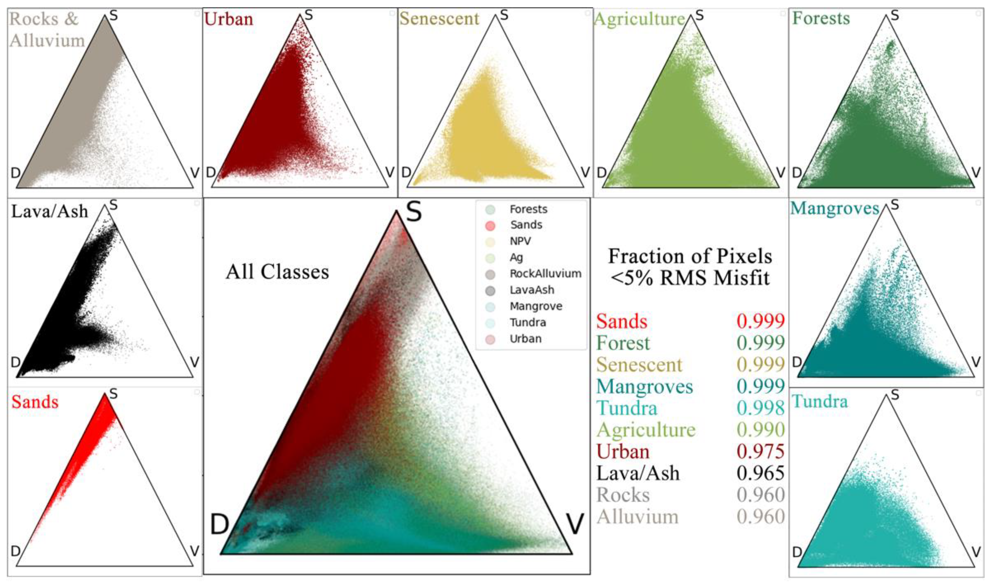
- What is the overall S,V,D fraction distribution of globally diverse representatives of significant land cover categories?
- How well does the global S,V,D model fit each land cover category, as measured by root mean square misfit?
Topological
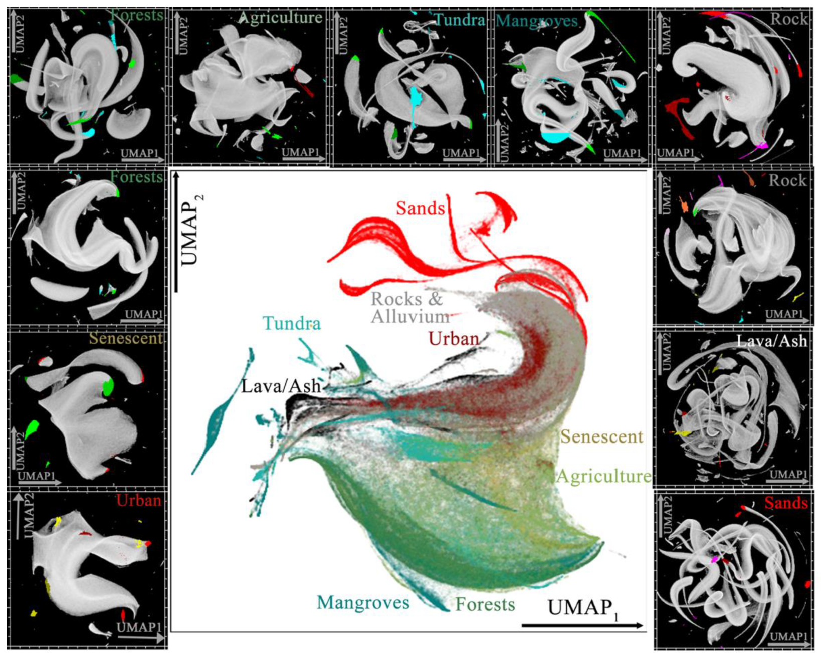
- How clustered or continuous are the manifolds for each land cover category found by UMAP?
Joint
- To what extent can S,V,D fractions and UMAP clusters be used together to yield useful information? Specifically,
  i.
  To what extent are UMAP clusters geographically contiguous?
  ii.
  To what extent do disparate UMAP clusters at similar S,V,D fraction values represent physically plausible and/or spectroscopically interpretable spectral variability?
  iii.
  Are some S,V,D fractions, or land cover classes, better suited to JC than others? If so, why? If not, why not?

2. Materials and Methods

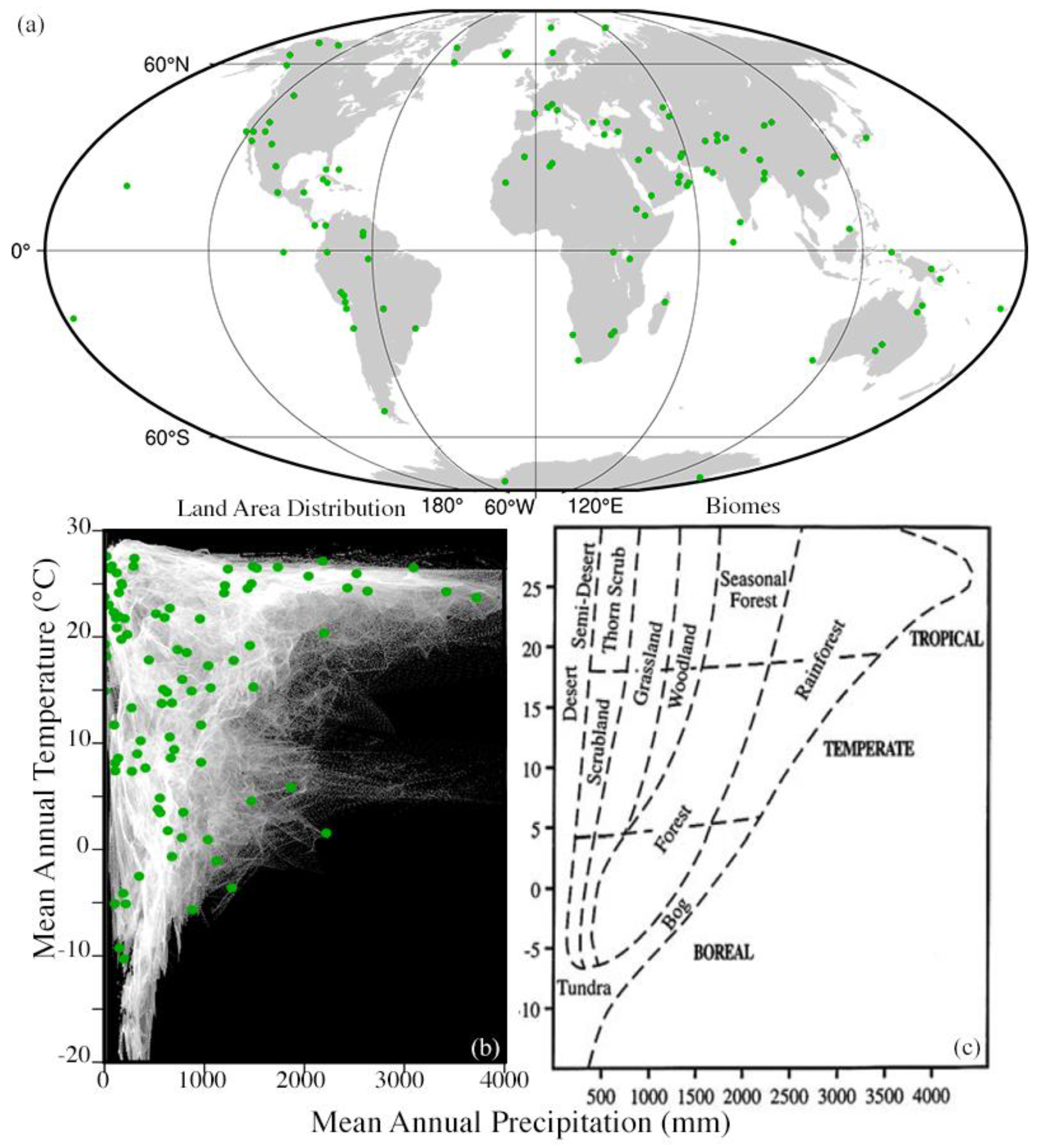
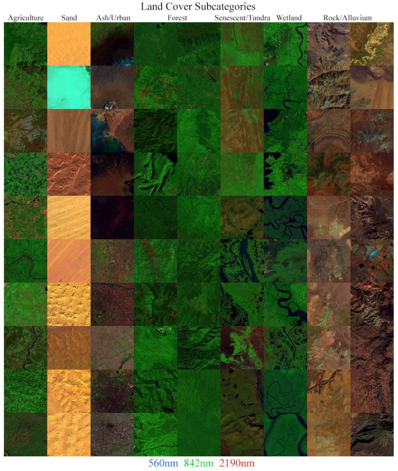
2.1. Data

110 Sentinel-2 image tiles were acquired as Level 1C exoatmospheric reflectance from the USGS EarthExplorer data portal (https://earthexplorer.usgs.gov/; accessed on 1 October 2022). Sites were selected to span a broad geographic diversity, sampling all major biomes and a wide range of geologic histories (Figure 1).

90 subsets were selected as representatives of dominant land cover classes. Each subset covered a 10 × 10 km (1000 × 1000 pixel) area dominated by a particular land cover class. The classes used were: agriculture, sand, lava/ash, urban, forest, senescent vegetation, tundra, wetland/mangrove, and rock/alluvium. For the agriculture, sand, wetland/mangrove, and rock/alluvium classes, 10 representative subsets of each were used. For the lava/ash, urban, senescent vegetation, and tundra classes, 5 subsets were used. For the forest class, 20 subsets were used and subsequent analysis was decomposed into two 10-tile portions. The full mosaic is shown in Figure 2 as a false color composite (R/G/B = SWIR/NIR/Visible). Scene IDs, UTM zones, and northwest corner Eastings and Northings for each subset are listed in Table A1.

Tile selection was based on spectral diversity of land cover, both within and among image tiles. Guided by previous global compilations (e.g., [36,37,38,39]), the collection of 110 Sentinel 2 tiles focused on spectral diversity hotspots spanning all of Earth’s biomes (Figure 1). As explained in detail by [32], maps of plant biodiversity, bedrock lithology, soil type and climatic zone were used to maximize the land cover diversity included in the compilation. In addition, agricultural crop diversity and urban morphologic heterogeneity guided the selection of anthropogenically modified landscapes. As verified by [32], the spectral dimensionality and topology of the 90 subset land cover subcategory mixing space is nearly identical to the larger 110 tile mixing space it represents.

As in [32], Sentinel 2 bands 1–8a, 11 and 12 were coregistered and resampled to 10 m resolution by linear interpolation. For hyperparameter tuning, the 90 land cover subcategory examples were mosaiced and spatially decimated by a factor of 10 in each dimension to reduce redundancy from spatial autocorrelation. This subsampling does not impact the spectral dimensionality or topology of the mixing space, but it does reduce the computational load of the nonlinear manifold learning (UMAP, t-SNE and Laplacian Eigenmap) while facilitating hyperparameter sweeps. Once final hyperparameters were chosen, UMAP was run again on each compilation at full resolution (without decimation).

2.2. Methods

The joint characterization workflow proceeded with the following three steps:

Use a linear spectral mixture model to characterize the overall S,V,D distribution of each land cover class (variance-based, physical, linear).
Use Uniform Manifold Approximation and Projection (UMAP; [33]) to characterize interdimensional topology & clustering (topology-based, statistical, nonlinear)
Synthesize Steps A and B into a set of 1 or more bivariate distributions which use the physical meaning of the Step A fraction distributions to differentiate among purely topological relations identified from Step B (joint characterization).

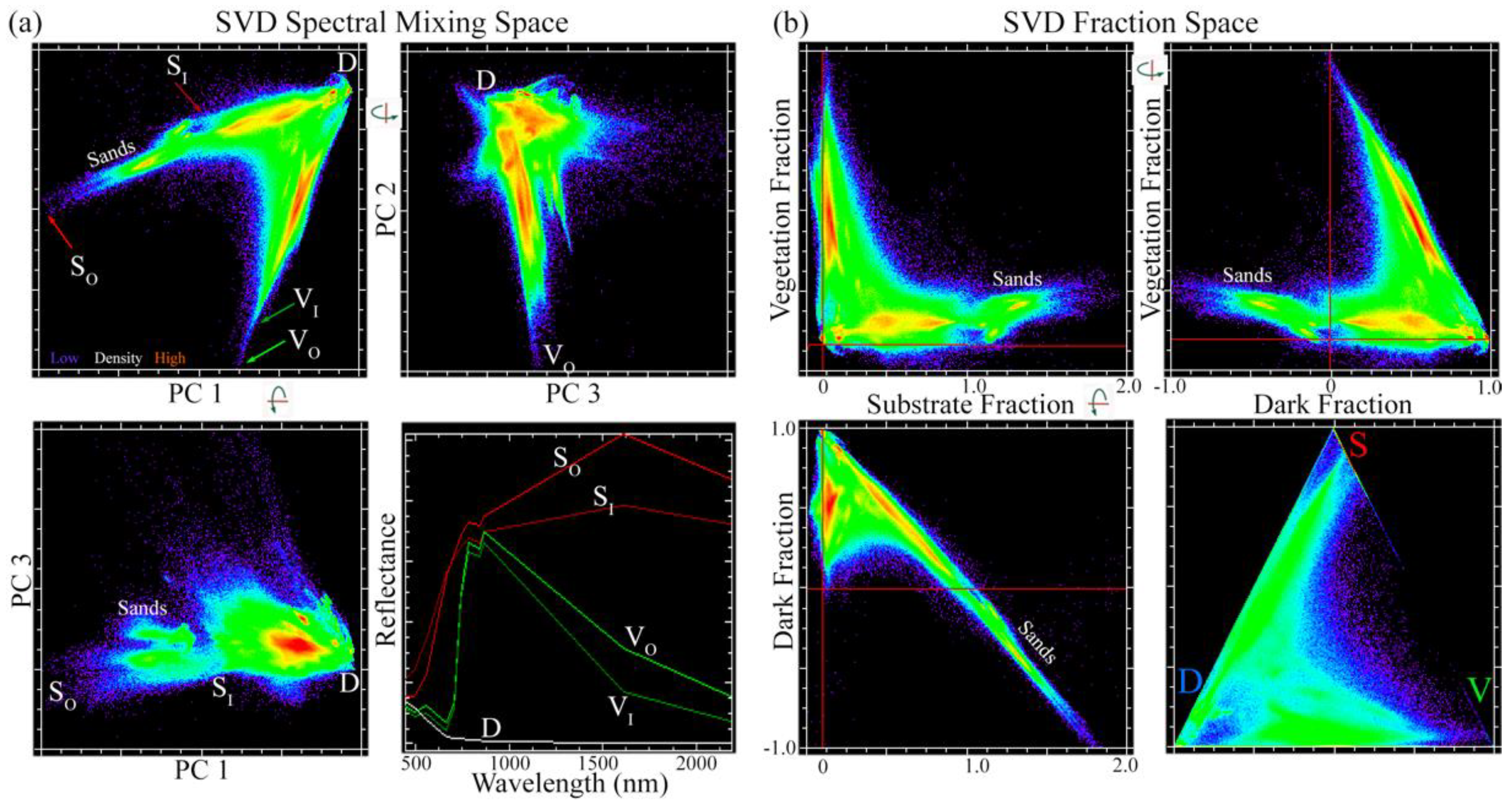
Spectral signatures of clusters identified from Step C were identified, region of interest (ROI) means and spectral separability metrics were computed, and geographic coherence was visually evaluated.

Each step is explained briefly below.

2.2.1. Step A: Linear Characterization and Modeling: Spectral Mixture Analysis

For the linear component of this analysis, the spectral feature space of the 90-tile mosaic was characterized using Principal Component Analysis [17] (Figure 3a) as described by [32]. Consistent with numerous studies with other multispectral and hyperspectral sensors [36,37,38,39,40,41], the preponderance of variance was found to be well-characterized by a small number of dimensions (95% of variance in the first 2 dimensions; 97% in the first 3 dimensions). Additionally, consistent with previous studies, the low-order spectral feature space of this diverse mosaic was found to be well-represented by linear mixing among Substrate, Vegetation, and Dark (S,V,D) spectrally distinct endmembers (EMs). Two sets of endmembers were selected, identifying both: (1) the “outer” (subscript O) convex hull bounded by the most extreme pixel spectra, and (2) the “inner” (subscript I) convex hull which excludes the most extreme spectra and uses 10- to 100-pixel mean spectra from the more densely populated region of each apex. All tiles were then unmixed to S,V,D fractions using the lower amplitude mean (S_I,V_I,D) endmembers [32]. Bivariate fraction distributions (Figure 3, right) show fraction estimates to be within the physical range (0 to 100%) for all tiles except high albedo sands, which give S_I fractions greater than 100% and D fractions less than 0. Mixture model misfit, as quantified by the Root Mean Square Error (RMSE) of misfit between observed and modeled spectra, was less than 6% for over 99% of spectra. Due to the unit sum constraint and the fact that the 3D SVD space maps onto a linear 2D subspace, fraction distributions can also be visualized using a barycentric plot (i.e., ternary diagram) with no loss of information. The remainder of this analysis uses such a visualization to demonstrate variability in S,V,D fraction abundance among land cover classes. For greater detail on variance-based characterization of this mosaic, see [32].

The fundamental principle underlying the S,V,D model is the observation that most decameter terrestrial pixels measure an aggregate of reflected (or scattered) radiance originating from more than one target. This is formalized by a linear spectral mixture model [20,21,22] which can be written as the vector equation

x = Mf + e

(1)

where x is the observed reflectance (or radiance), M is the matrix of spectrally distinct endmember reflectances (or radiances), f is the vector of subpixel area fractions of each endmember, and e is a vector of errors [42].

Specifically, the generalized S,V,D model used in this study takes advantage of the observed generality of Earth’s (terrestrial, non-cryospheric, non-evaporitic) reflectance field as being well-characterized by linear combinations of three stable Substrate, Vegetation, and Dark endmembers [36,43,44].

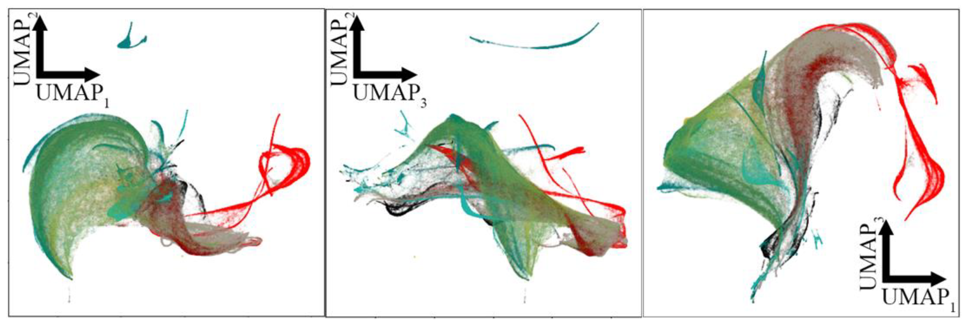
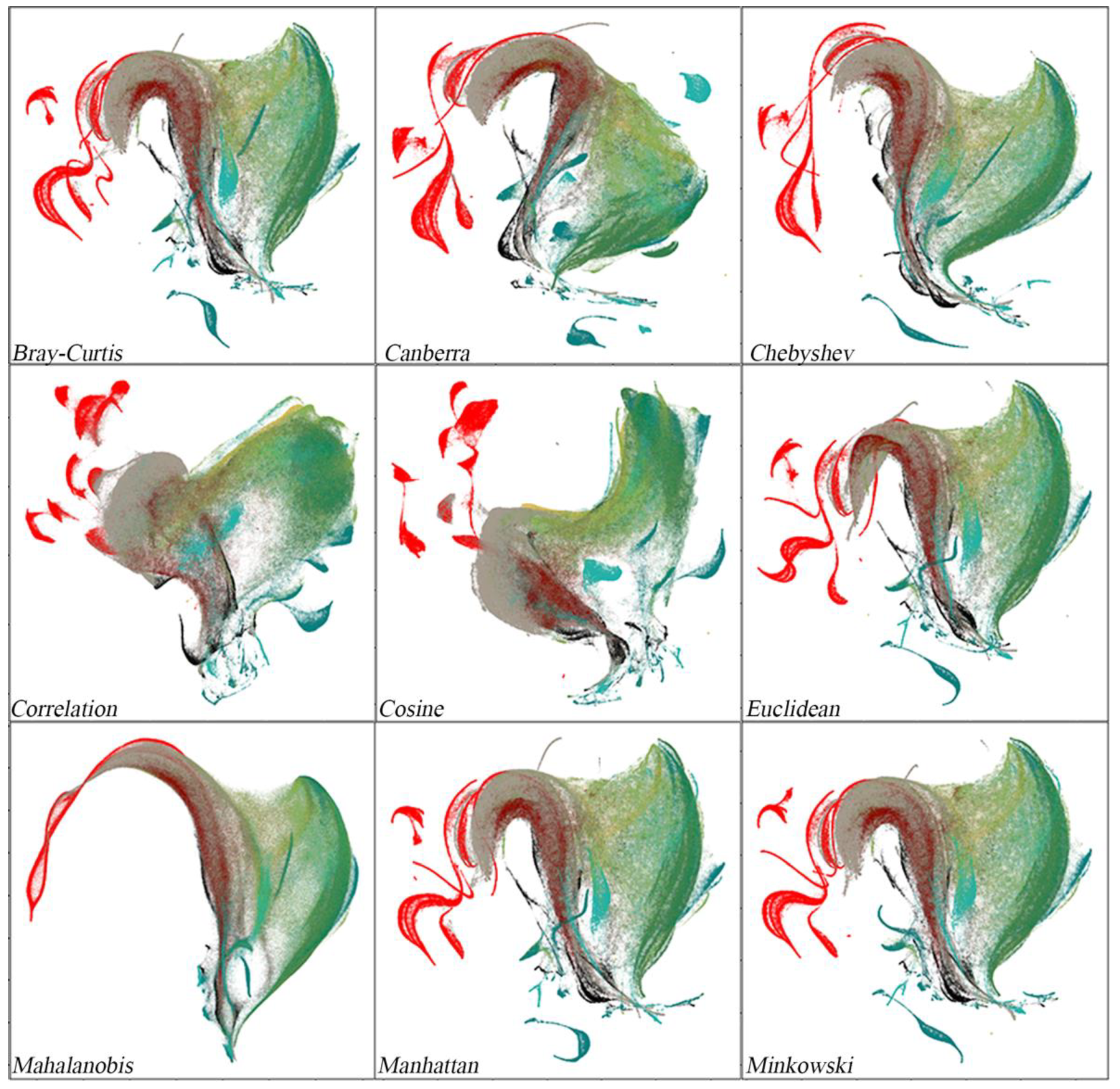
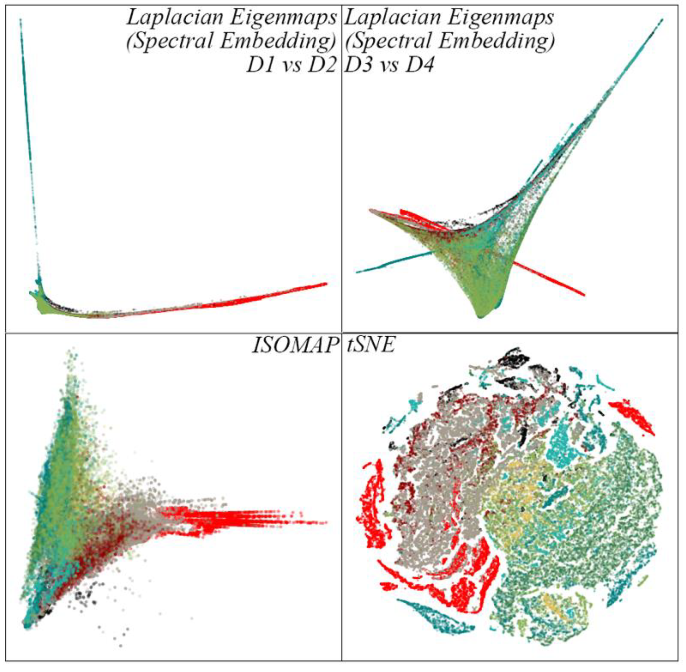
2.2.2. Step B: Nonlinear Characterization and Modeling: Manifold Learning

In this analysis, nonlinear characterization was based on Uniform Manifold Approximation and Projection (UMAP) [33] of the 11D spectral mixing space. UMAP is a novel, increasingly popular algorithm for nonlinear dimensionality reduction. Mathematically, UMAP assumes that the Sentinel-2 spectra are uniformly distributed on a locally connected Riemannian manifold with an (approximately) locally constant Riemannian metric. UMAP models this manifold using a fuzzy topological structure, then seeks a low-dimensional (usually 2 or 3D) embedding with an optimally similar fuzzy topological structure. The resulting embedding is generally nonlinear and noninvertible.

UMAP results depend on choice of several tunable hyperparameters. Among the most important are:

-: n_components: The number of dimensions of the low-D embedding space.
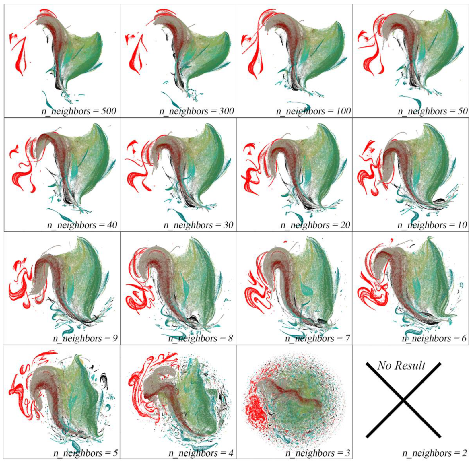
-: n_neighbors: The size of the local neighborhood used when learning the manifold structure of the data.
-: min_dist: The limit on how closely points may be spaced in the output space.
-: metric: The distance metric in the input space.

For all figures in the following analysis, we use the following values:

-: n_components = 2
-: n_neighbors = 30
-: min_dist = 0.1
-: metric = Euclidean

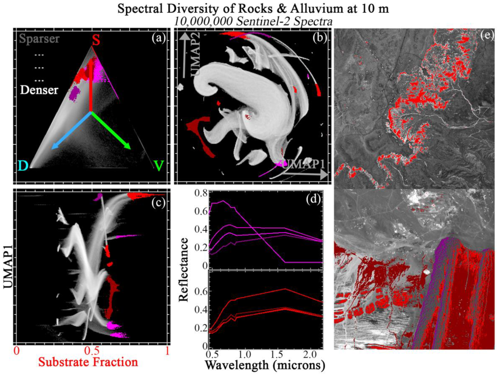
For the sake of presentation, we defer an illustration of dependence on hyperparameter setting to the (Figure A1, Figure A2, Figure A3, Figure A4 and Figure A5).

All UMAP computations were performed using the open source umap-learn Python package on a commercially available laptop computer with 32 GB RAM, 2GHz Quad-Core Intel Core i5 CPU, and a 1536 MB Intel Iris Plus Graphics GPU. Runtime for a typical 10 tile (10,000,000 11-band spectra) subset was approximately 2 hours. For more information about UMAP, see [45].

2.2.3. Step C: Joint Characterization: Bivariate Distributions and Cluster Identification

Linear and nonlinear methods were then combined to perform a joint characterization of the spectral mixing space. In this analysis, we implement JC using bivariate distributions of the linear and nonlinear mixing space characterizations. This step leverages interrelationships between the variance-based (spectral mixture fraction) and topology-based (UMAP embedding) metrics.

In the context of this analysis, the mutually reinforcing goals of JC are to: (1) use the mixture fractions to imbue the UMAP embedding with physical meaning, and likewise (2) to use the UMAP embedding to differentiate between subsets of otherwise apparently continuous, indistinct mixture fractions.

Conceptually, JC follows approaches like [46,47] in seeking a robust analytic framework capable of both (a) exploiting (potentially) high dimensional and/or nonlinear signals, and (b) adhering to the well-known physical constraints of linear mixing processes. The chief novelty is in the fusion of recent developments in manifold learning with a now well-established low-order global S,V,D spectral mixing space.

In the subsequent analysis, spectral endmember fractions are shown on the x-axis and UMAP embedding is shown on the y-axis. Different endmember fractions are more or less useful for understanding different land cover types, so the choice of S, V, or D endmember used in the following JC plots is dependent on the land cover subcategory.

3. Results

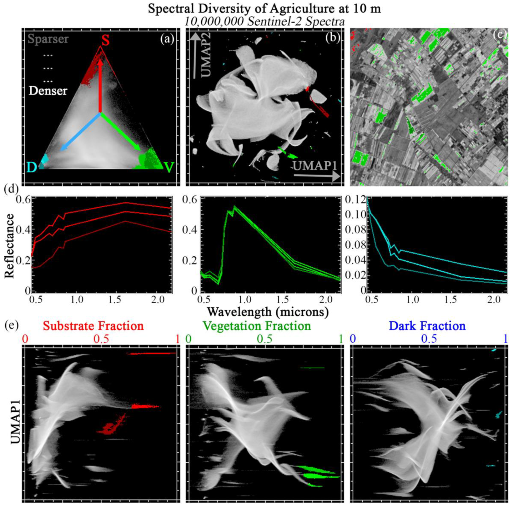
3.1. Agriculture

Figure 4 illustrates the JC workflow as applied to a compilation of 10 tiles from diverse agricultural basins worldwide. From the SVD ternary diagram (top left), we see that this collection spans nearly the entire global mixing space. These spectra are well-fit by the global mixture model (99% spectra with <5% RMSE). Pixels with fractions near 1.0 are observed for each endmember. Both S ↔ D and D ↔ V binary mixtures are observed. Consistent with previous studies, the edge of the space corresponding to S ↔ V binary mixing is much sparser due to the ubiquity of subpixel shadow in even the flattest and smoothest natural landscapes.

The 2D UMAP embedding (top center) suggests that most of the geographic area is well-represented by a single broad, well-connected manifold, but several exceptions are also present in the form of both apexes to the main manifold and smaller pixel clusters disconnected from the main manifold. Joint Characterization (bottom row) shows this useful manifold structure can be present at high fractions for all three S,V,D endmembers. ROI mean spectra with high S endmember fractions show plausible differences in soil moisture, albedo, and/or composition. Dominant variability in JC-identified V endmembers corresponds predominantly to SWIR1 (suggestive of leaf water) and visible bands (suggestive of differences in pigments). Variability in JC-identified D endmembers largely corresponds to overall brightness in the NIR and SWIR (turbidity, flotsam?) and curvature in the visible (chlorophyll, CDOM?).

All endmembers were identified as ROIs from the JC plots. These ROIs were then back-projected onto both the ternary diagram and UMAP plot, and visualized in geographic space for 1 example tile from the 10 comprising this land cover compilation (top right). Geographic coherence (e.g., spatial clusters conforming to visually distinct intra- and inter-field boundaries) strongly implies that the ROIs are likely to have physically meaningful distinctions. Examination of the back-projected ROIs on the ternary diagram shows that they would clearly not be distinct from examination of S,V,D fractions alone; examination of the ROIs on the UMAP plot shows that they would have no physically interpretable context from UMAP alone.

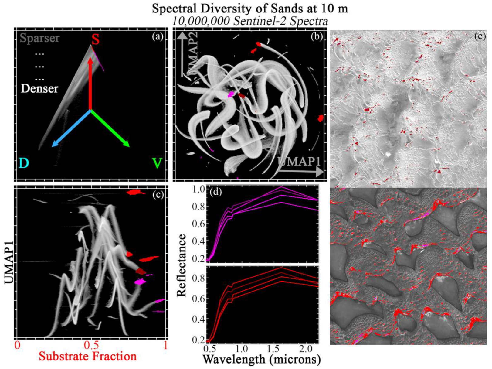
3.2. Sands

Figure 5 shows JC applied to a compilation of 10 tiles collected from geologically diverse sand dunes. As expected, the SVD ternary diagram (top left) shows a strong preferential distribution towards the global S endmember, with most mixing occurring along the S ↔ D binary mixing line. Pixels with substantive V endmember contributions are effectively absent as few plants can grow in pure sand substrate. The sand spectra are well-fit by the global mixture model (99.9% spectra with <5% RMSE)—but fractions regularly exceed 100% due to frequently being brighter than the global soil endmember because of high solar incidence angle on sun-facing dune slopes. This suggests that differences between these spectra and the global S spectrum are largely driven by scaling of overall brightness, and not major changes in spectral curvature.

Examination of 2D UMAP embedding (top center) shows a discontinuous, sinuous manifold with numerous apexes and exterior pixel clusters. For JC of this land cover compilation, the S endmember fraction is the obvious choice for JC of this land cover compilation (bottom left).

Many high S distinct clusters are clearly identifiable from JC. 8 illustrative examples are shown in red and magenta. ROI mean spectra (bottom center) show variability consistent with potential physical drivers like grain size and mineralogy. Here, the S fraction effectively stratifies UMAP clusters by albedo, and UMAP effectively differentiates among subtle differences in spectral curvature among sands with similar albedos.

ROIs are geographically visualized on 2 example tiles (right column). ROI pixels consistently cluster on the basis of topographic position and geographic location in ways that strongly suggest physical meaning (e.g., fine vs. coarse grain size at troughs vs. dune crests). ROIs are again also back-projected onto both the SVD and UMAP spaces. From this back-projection, the complementarity captured by JC is again evident: UMAP clusters without EM fraction context lack physical context, and EM fractions without UMAP are visually indistinct.

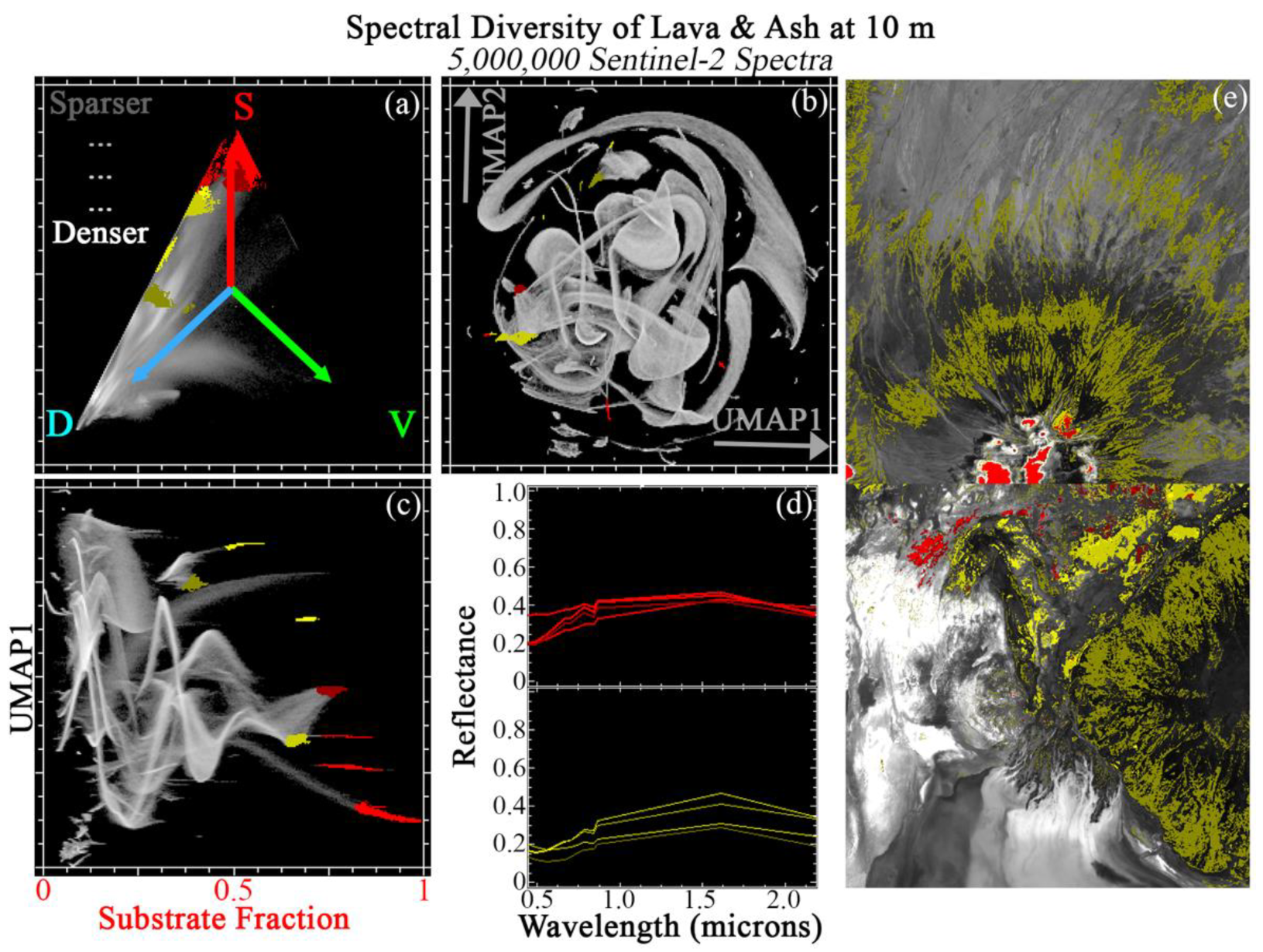
3.3. Lava and Ash

Figure 6 shows JC applied to a compilation of 5 tiles from globally diverse volcanic (lava and ash) landscapes. Within the global SVD mixing space, these landscapes are preferentially distributed between the D and S endmembers (top left). Some substantive mixing towards the V EM is also observed. Relative to the other land cover classes, these spectra are not particularly well fit by global mixture model (96.5% spectra with <5% RMSE). Presumably, this is because the global D endmember corresponds to clear, deep water—not ferromagnesian rock (e.g., basalt).

Examination of 2D UMAP embedding (top center) shows a set of interconnected submanifolds, each with numerous apexes and exterior pixel clusters. The S endmember fraction is again used to illustrate JC of this land cover compilation (bottom left).

Again, many distinct clusters with moderate to high S fraction are clearly identifiable from the JC. 8 of the clearest are shown in red and yellow. These ROIs are differentiated in terms of both overall albedo and spectral curvature across the full visible through shortwave infrared (VSWIR) range. The observed spectral variability is suggestive of differences in underlying (mafic: felsic) mineralogy, mineral vs. glass composition (holocrystalline ↔ holohyaline), texture (aphaneritic ↔ phaneritic), and lava flow age/weathering.

ROIs are geographically visualized on 2 example tiles (right column). ROI pixels consistently cluster on the basis of topographic position and geographic location in ways that strongly suggest geophysical meaning (e.g., topographic position, across vs. within individual flow extents). Back-projection of ROIs onto both SVD and UMAP spaces again highlights the complementarity of each characterization approach.

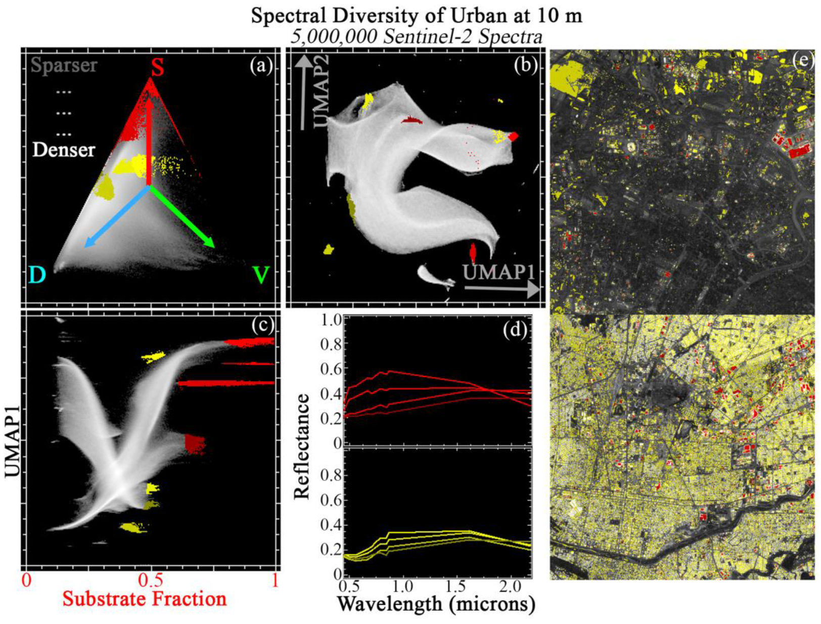
3.4. Urban

Figure 7 shows JC applied to a compilation of 5 tiles from globally diverse urban landscapes. Within the global SVD mixing space, these landscapes are preferentially distributed between the D and S endmembers (top left). More mixing towards the V EM is observed than with the volcanic or sand land cover classes. These spectra are better fit by the global mixture model than the volcanic compilation, but worse fit than the agriculture or sands (97.5% spectra with <5% RMSE).

Examination of 2D UMAP embedding (top center) shows a single, highly connected main manifold, with numerous apexes. This manifold is much more continuous than for the preceding land cover classes, with more dominant global structure and less prominent statistically local clustering. The S endmember fraction is again used to illustrate JC of this land cover compilation (bottom left).

Again, many distinct clusters are clearly identifiable from the JC. 8 of the clearest are shown in red and yellow. These ROIs are differentiated in terms of both overall albedo and spectral curvature across the full VSWIR range, particularly in the infrared spectral region. The observed spectral variability is suggestive of differences in synthetic materials (plastics, asphalt, roofing materials, paint), as well as exposed substrates.

ROIs are geographically visualized on 2 example tiles (right column). ROI pixels consistently cluster in ways suggestive of physical meaning (parking lots, roofs of large buildings, city blocks). Back-projection of ROIs onto both SVD and UMAP spaces again highlights the complementarity of each characterization approach.

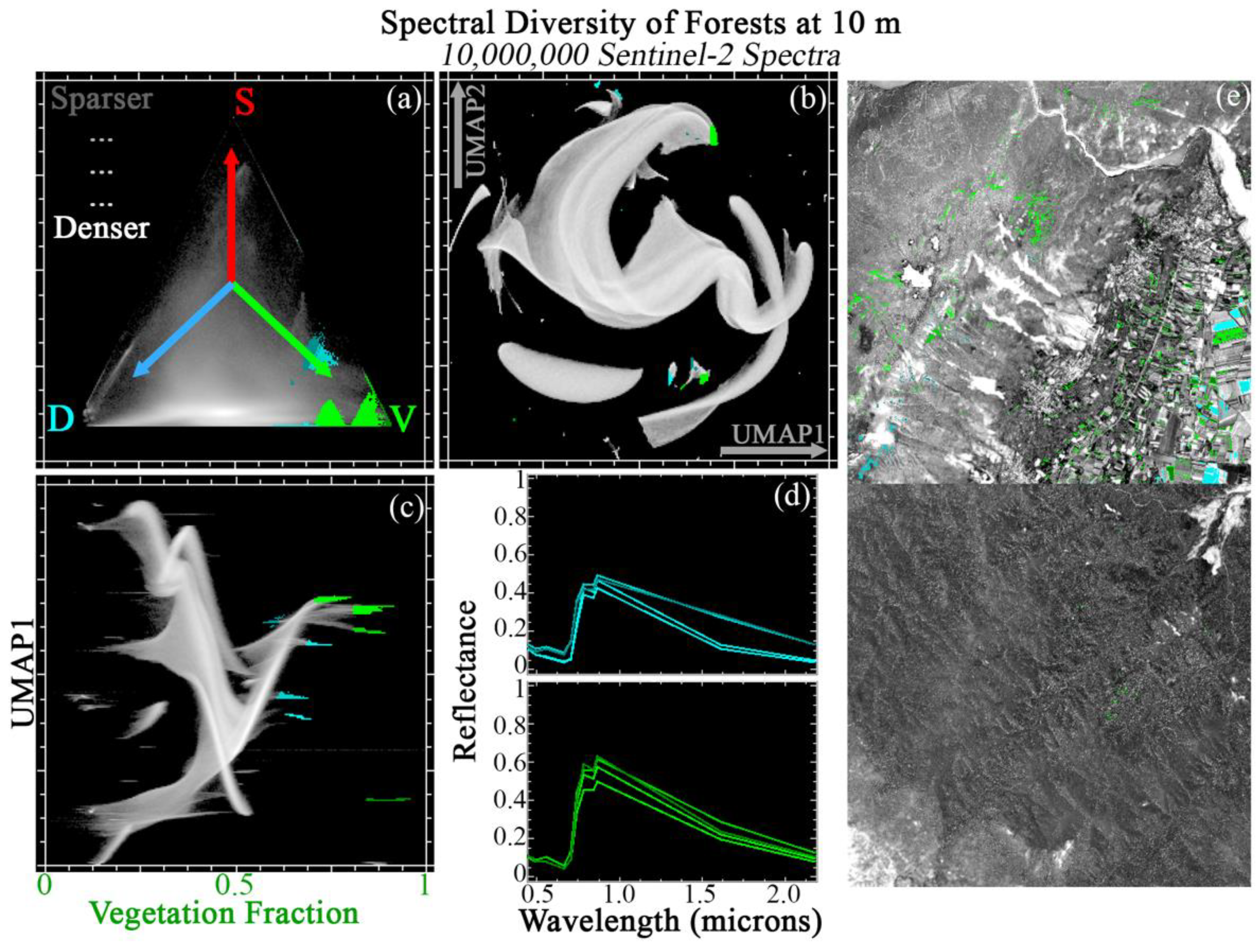
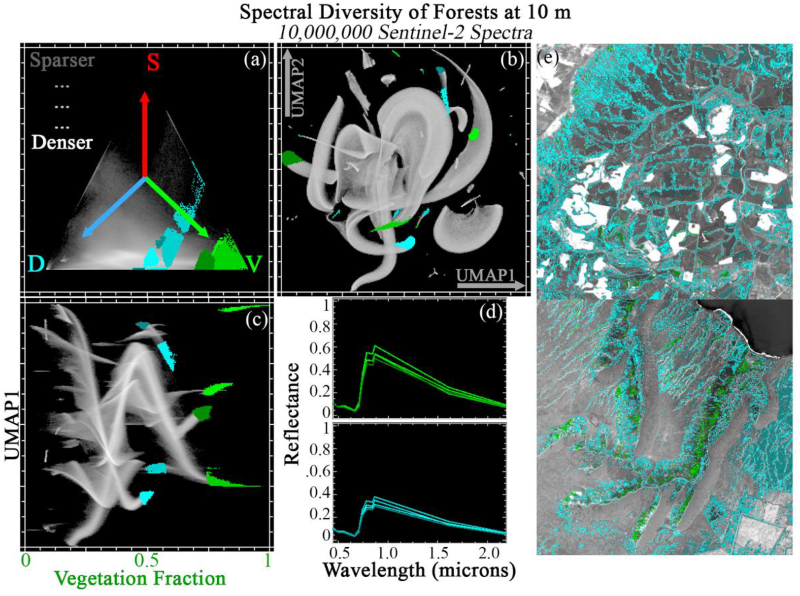
3.5. Forests

Figure 8 and Figure 9 show JC applied to a compilation of 20 tiles (2 sets of 10) from globally diverse forests. Forest spectra are preferentially distributed towards the D ↔ V mixing line (consistent with closed canopy spectra), with a significant amount of additional mixing towards S (consistent with incomplete canopy closure, stems and other woody material, and/or senescent leaves). The forest spectra are better fit by the global SVD mixture model than any preceding land cover class (99.9% spectra with <5% RMSE).

The 2D UMAP embedding (top center) shows a broad, well-connected manifold comprised of several major lobes. This manifold is visually less continuous than Urban, but more continuous than Sands or Lava/Ash. Multiple apexes to the main manifold and smaller disconnected pixel clusters are also present.

The V fraction is the natural endmember to use for Joint Characterization (bottom left). Useful manifold structure is observed at a wide range of V fractions. In each figure, 8 of the clearest are shown in cyan and green. These clusters are differentiated in terms of NIR amplitude (e.g., leaf structure), visible wavelength slope and curvature (e.g., pigments), and overall SWIR brightness (e.g., leaf water & dry matter).

In each figure, ROIs are geographically visualized on 2 example tiles (right column). As with other land cover classes, geographic clustering of ROIs (microtopography, distance from channel, ecological differences among tiles) implies plausible geophysical meaning. Back-projection of ROIs onto both SVD and UMAP spaces again highlights the complementarity of each characterization approach.

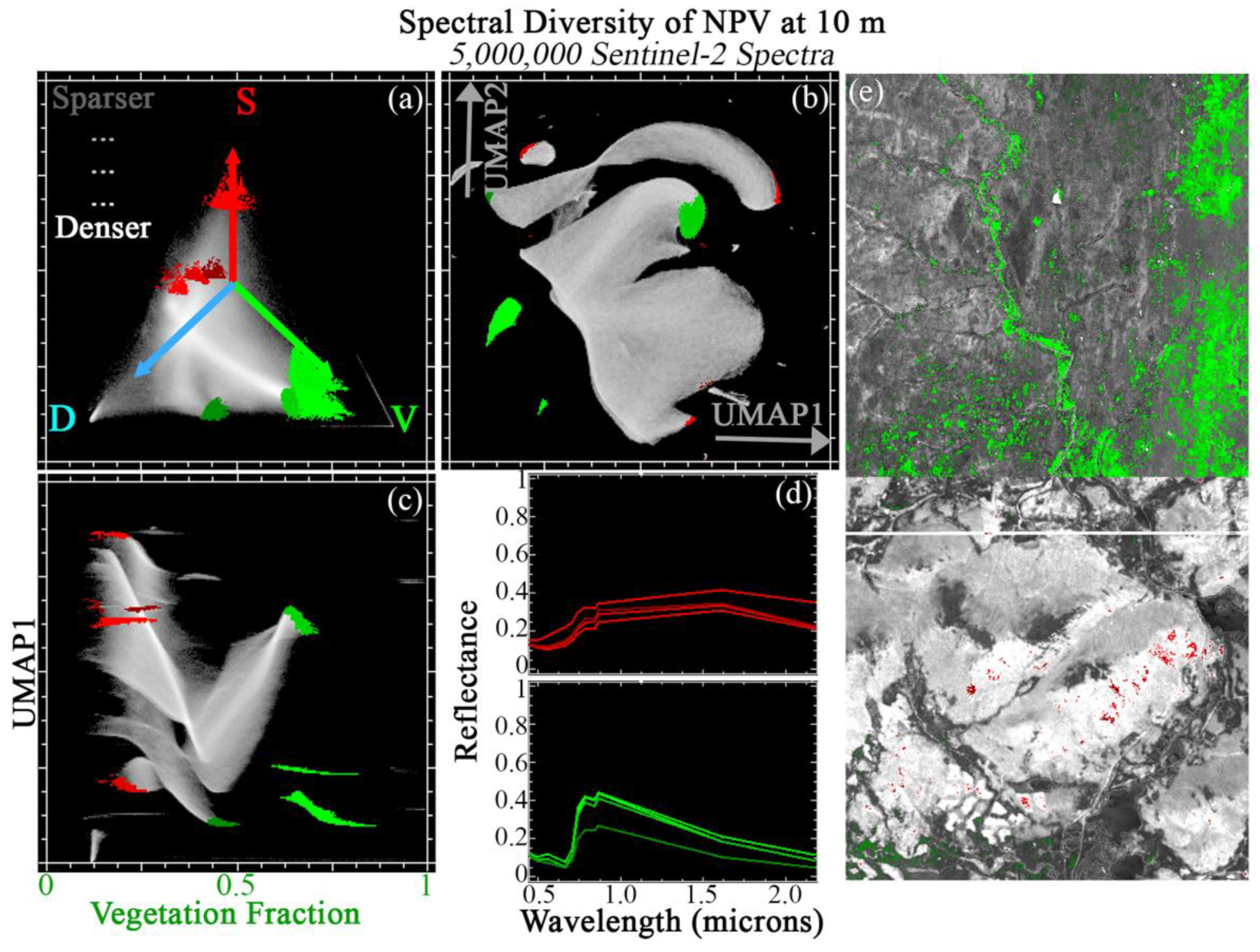
3.6. Senescent Vegetation

Figure 10 shows JC applied to a compilation of 5 tiles from diverse biomes dominated by senescent (non-photosynthetic) vegetation. Within the global SVD mixing space, these landscapes are preferentially distributed towards high- to mid- Dark fraction values, with mixing towards both V and S endmembers well-represented, but less comprehensive than for the agriculture compilation (top left). Like the forest compilations, these spectra are also well fit by the global mixture model (99.9% spectra with <5% RMSE).

Examination of 2D UMAP embedding (top center) shows a single, highly connected main manifold. This continuity of this manifold is comparable to that of the urban land cover compilation. The V endmember fraction is again used to illustrate JC of this land cover compilation (bottom left).

Again, many clusters are clearly identifiable from the JC. 4 of the clearest V-dominated clusters are shown in green. 4 additional S-dominated clusters were selected from the S-based JC (not shown) and projected onto the V-based JC space. S-dominated ROIs are differentiated in terms of differences in NIR brightness and associated curvature. V-dominated ROIs are differentiated in terms of red edge bands and SWIR, along with NIR brightness. The observed spectral variability is suggestive of differences in overall vegetation composition and 3D structure (e.g., differences in volume scattering associated with grass vs. shrub vs. tree morphologies), as well as stage of senescence. V-dominated ROI differences are suggestive of leaf water (SWIR) and leaf structure (red edge, NIR), with one cluster showing significant differences in visible wavelength curvature in addition to a 50% reduction in NIR brightness. ROIs are geographically visualized on 2 example tiles (right column), and again cluster in ways suggestive of biophysical meaning (along river channels, stands of trees, discernable savanna transitions).

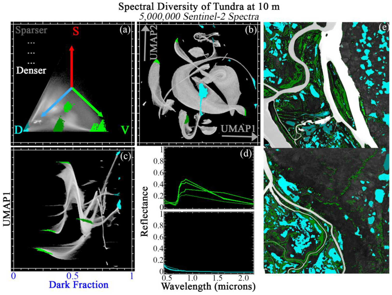
3.7. Tundra

Figure 11 shows JC applied to a compilation of 5 tiles from diverse tundra landscapes. Within the global SVD mixing space, these landscapes are preferentially the D ↔ V mixing line (consistent with dense vegetation and vegetation/water mixtures), with minor additional mixing towards S (consistent with dark, water-saturated soils) (top left). Like the forest and senescent vegetation compilations, these spectra are well fit by the global mixture model (99.8% spectra with <5% RMSE).

Examination of 2D UMAP embedding (top center) shows a single main manifold with several lobes. This manifold is less continuous than the urban or senescent vegetation compilations, but more continuous than the sand or volcanic compilations. Here, the D endmember fraction is used to illustrate JC of this land cover compilation (bottom left).

Again, many clusters are clearly identifiable from the JC. 4 of the clearest D-dominated clusters are shown in cyan. 4 additional low-D (and high V) clusters were also selected (shown in green). D-dominated ROIs are differentiated in terms of overall brightness in the NIR and SWIR (turbidity/flotsam?) and curvature in the visible (chlorophyll, CDOM?). V-dominated ROIs are differentiated in terms of NIR amplitude (plant community structure?), visible wavelength slope and curvature (pigments?), and overall SWIR brightness (canopy & understory water? Spatial mixing with underlying waterlogged substrate?). ROIs are geographically visualized on 2 example tiles (right column), and again cluster in ways highly suggestive of biophysical meaning (V: distance from river channel, microtopography, differences among tiles; D: sets of thermokarst lakes clustering together, possibly on the basis of lake age, largely distinct from river channels).

3.8. Mangroves and Wetlands

Figure 12 shows JC applied to a compilation of 10 tiles from diverse mangrove and wetland landscapes. Mixture fractions from these landscapes are distributed similarly to tundra, preferentially occurring near the D ↔ V mixing line, with minor additional mixing towards S (consistent with more open canopies resulting in subpixel mixing with water or dark, water-saturated soils) (top left). Like the forest, senescent vegetation, and tundra compilations, these spectra are well fit by the global mixture model (99.9% spectra with <5% RMSE).

Examination of 2D UMAP embedding (top center) shows a single main manifold with several lobes. This manifold also comparable to the tundra compilation: less continuous than the urban or senescent vegetation compilations, but more continuous than the sand or volcanic compilations. Here, the V endmember fraction is used to illustrate the JC approach (bottom left).

Again, many submanifolds are clearly identifiable as apexes and clusters from the JC. 8 of the clearest V-dominated clusters are shown in cyan and green. 4 additional low-D (and high V) clusters were also selected (shown in green). D-dominated ROIs are differentiated in terms of overall brightness in the NIR and SWIR (turbidity/flotsam?) and curvature in the visible (chlorophyll, CDOM?). V-dominated ROIs are differentiated in terms of NIR amplitude (possibly associated with leaf and canopy structure), visible wavelength slope and curvature (potentially associatd with pigments), and overall SWIR brightness (potentially associated with canopy and/or understory water, and spatial mixing with an underlying waterlogged substrate). ROIs are geographically visualized on 2 example tiles (right column), and again cluster in ways highly suggestive of biogeophysical meaning (distance from river channel, microtopography, differences among tiles).

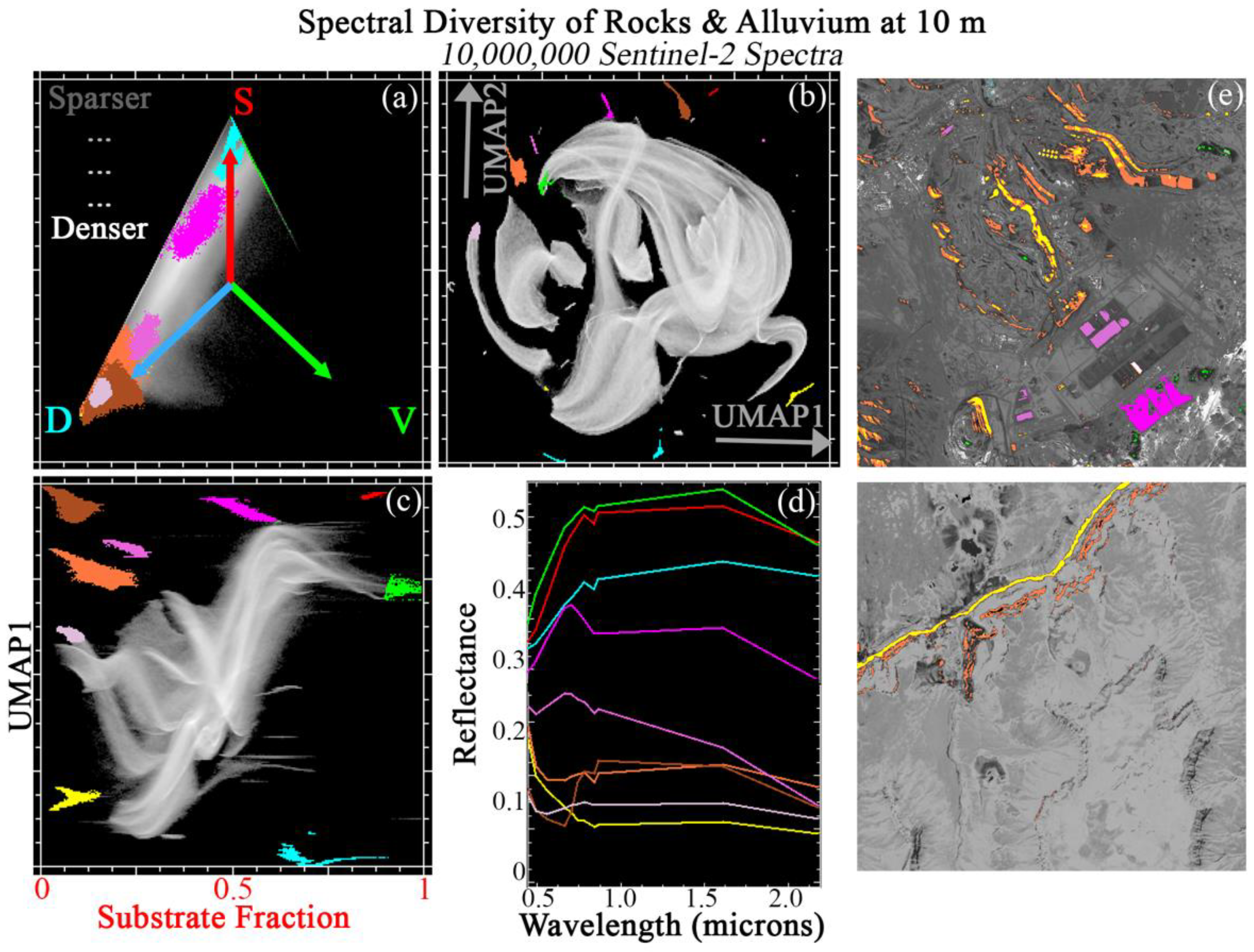
3.9. Rocks and Alluvium

Figure 13 and Figure 14 show JC applied to a compilation of 20 tiles (2 sets of 10) from geologically diverse landscapes exemplifying rock and alluvium, respectively. Both rock and alluvium spectra are preferentially distributed towards the D ↔ S mixing line, with minor mixing towards V within the global SVD mixing space (upper left). Like the lava/ash spectra, these spectra are less well fit by the global mixture model (96% spectra with <5% RMSE), presumably because the single Substrate EM does not capture the full geologic diversity of the basement rocks and alluvium.

The 2D UMAP embedding (top center) shows a broad, well-connected manifold comprised of several major lobes. These manifolds are visually less continuous than Urban, but more continuous than Sands or Lava/Ash. Multiple apexes to the main manifold and smaller disconnected pixel clusters are also present.

Here, the S fraction is the natural endmember to use for JC (bottom left). Useful manifold structure is observed at a wide range of S ↔ D mixture fraction continuum. In each figure, 8 of the clearest apexes and clusters are shown. These ROIs are differentiated in terms of both overall albedo and spectral curvature across the full VSWIR range. Mean cluster spectra are suggestive of differences in underlying (mafic: felsic) mineralogy, rock type (igneous, sed, met), exposure age/weathering, hydrothermal alteration, presence/absence of evaporite minerals.

In each figure, ROIs are geographically visualized on 2 example tiles (right column). As with other land cover classes, geographic clustering of ROIs (topographic position, relation to extraction operations) identified from JC implies plausible geophysical meaning. Back-projection of ROIs onto both SVD and UMAP spaces again highlights the complementarity of each characterization approach.

4. Discussion

With these results in mind, we structure our discussion in three parts. First, we revisit each fundamental science question that motivated the analysis. Next, we present a conceptual explanation for the efficacy of the method. We then close with a brief discussion of limitations, avenues for future work, and concluding remarks.

4.1. Revisiting the Motivating Questions

4.1.1. Question 1: Variance-Based Characterization & Modeling

The first set of questions addressed by this study concerned the overall SVD fraction (and misfit) distributions of globally significant land cover classes. The SVD fraction question is addressed by the ternary diagrams shown in the upper left of each of Figure 4, Figure 5, Figure 6, Figure 7, Figure 8, Figure 9, Figure 10, Figure 11, Figure 12, Figure 13 and Figure 14. We summarize these in Figure 15, showing the SVD distribution for each category (outer plots), as well as the merged global distribution of the entire mosaic (center left). Clearly, the land cover categories used in this study occupy overlapping subsets of the global SVD space. This is in part because spectral mimicking may render distinct reflectances indistinguishable with a broadband sensor, and in part because not all categories are fully mutually exclusive. For example, some rock and alluvium subsets certainly contain some amount of green and senescent vegetation, as well as some sand; and clear decision boundaries are not always present among the wetland, mangrove, and forest categories.

Despite this fundamental nonuniqueness observed in SVD fraction space, differences among land cover category distributions are also evident. Specifically, agricultural landscapes (light green) are the most spectrally variable of all the categories, spanning nearly the entire space SVD space. Forests, mangroves, tundra (dark green, dark cyan, and cyan, respectively) are reasonably well mixed, but preferentially occur towards the D ↔ V binary. Urban landscapes (dark red) are also reasonably mixed, but instead skew towards the D ↔ S binary. Rocks, alluvium, and lava/ash (dark gray, dark brown, and black) are further skewed towards the D ↔ S binary, and the sands used in this compilation (red) demonstrate this preferential distribution even more strongly.

Mixture model misfit also varies by land cover category (Figure 15, center right). Categories dominated by closed canopies, exposed soil, and water tend to yield relatively low misfits (5% error or less for >99% of pixel spectra). Categories with the highest misfit are likely to host greater substrate diversity than can be captured by a simple 3 EM model. This is to be expected as the variance in PC 3 is almost entirely associated with the broadening diversity of substrates approaching the Dark endmember. Because the SVD model corresponds to a planar triangle, most of these substrates lie outside the model and project onto the SVD plane at its nearest point. This misfit can take the form of either geologic (rock, soil, alluvium, lava/ash) or synthetic (urban) materials. Notably, even for these poorer-fit landscapes, the vast majority (>95%) of pixels still show root mean square misfits < 5%.

4.1.2. Question 2: Topology-Based Characterization & Modeling

The second set of questions concerns category dependence of the underlying topology of the spectral data manifold. These questions are addressed by the UMAP manifolds in the top center of each of Figure 4, Figure 5, Figure 6, Figure 7, Figure 8, Figure 9, Figure 10, Figure 11, Figure 12, Figure 13 and Figure 14, summarized for convenience along the periphery of Figure 16.

Spectral manifold topology can clearly vary considerably across land cover types. In some cases, UMAP learns a single, well-connected manifold with a relatively small number of apexes and exterior clusters (e.g., Urban, Senescent Vegetation). In other cases, substantially more sinuous manifolds are found with more complex apexes and disconnected exterior clusters (e.g., Sands, Lava/Ash). Other land cover classes yield intermediate results.

4.1.3. Question 3: Leveraging Variance & Topology with Joint Characterization

The third set of questions we address concerns the practical utility of the joint (SVD + UMAP) characterization approach. These questions are addressed by the joint characterization plots and associated spectra shown in the lower portion of Figure 4, Figure 5, Figure 6, Figure 7, Figure 8, Figure 9, Figure 10, Figure 11, Figure 12, Figure 13 and Figure 14, and geographic patterns shown in the right columns. For brevity, these are not summarized in an additional figure here.

Clearly, JC consistently succeeds in using SVD fractions to differentiate UMAP clusters on the basis of physical interpretability. JC-identified ROIs frequently demonstrate geographic coherence and spectral interpretability from (putative) absorption features and scattering processes. In addition, JC produces potentially useful results even though overall spectral variance, spectral curvature, geographic size/contiguity of landscape features, and generative physical processes vary considerably across land cover types. Further, JC seems to be equally effective at capturing potentially useful clustering relations when landscapes are dominated by either S, V, or D endmember fractions. We speculate that the ability of JC to capture clustering relations across all three endmember fractions may arise from the stability of the three component linear model in conjunction with the sensitivity of UMAP to statistically local neighborhoods without regard to overall brightness or spectral shape. We expand further on this critical convergence of stability and sensitivity in the following subsection.

4.2. Why JC Works: A Convergence of Visions

The preceding analysis clearly demonstrates that JC is effective at identifying subtle, spatially coherent, spectrally distinct patterns in multispectral imagery. However, why does this approach work? Here, we present the philosophy underlying the approach in the context of two complementary visions for analysis of high dimensional imagery.

4.2.1. The Geophysical Vision: Projecting Each Pixel Spectrum Independently onto the Global Mixing Space

One vision for the analysis of spectral imagery conceptualizes the problem geophysically. This approach is rooted in a long history of physically based characterization and modeling approaches which has been formalized by the field of geophysical inverse theory [48,49,50]. In the context of the present study, this framework considers the image analysis problem to be physical, linear, and deterministic. A specific, interpretable quantity is estimated (e.g., area contribution of constituent EMs). Some prior knowledge of the system is required—which fortunately has been obtained by previous studies characterizing the global spectral mixing space ([36,43,44] and subsequent papers). This knowledge is used to design a system of equations which can be formulated into a matrix which describes a specific set of linear mixing processes governing the interaction of incident solar radiation with the Earth surface. Only 1 tunable parameter (weight of unit sum constraint) is present, and the rationale for parameter choice (1.0) has quasi-physical basis. This assumption is intrinsically linked to the choice of error metric (or cost function), which is commonly selected as the l₂ norm. Inverting the linear mixture model to obtain estimates of EM fractions provides a continuous result that is easily validated by comparison with higher spatial resolution imagery (vicarious validation) or in situ field measurements. A key assumption of this approach is that global variance is representative of information content.

4.2.2. The Statistical Vision: Learning High-Dimensional Structure within and among Clusters of Similar Pixel Spectra

Another vision for the analysis of spectral imagery conceptualizes the problem purely statistically. This approach is rooted in the more recently developed field of manifold learning, e.g., as reviewed by [16] and implemented for hyperspectral image analysis by [51,52]. Here, no a priori physical model is assumed. Linearity is also not assumed, and models generally have a stochastic element. The problem of characterization is formulated in terms of estimation of an abstract quantity (i.e., optimal embedding of a natively high-D manifold into a low-D space). Prior geophysical knowledge is not required, nor is it used. Several tunable parameters exist, which can significantly alter the output. Often a parameter is used to quantify connective complexity by setting a number of statistical neighbors to be examined. In this context, hyperparameter choice is less defensibly physical (although arguments can be made for a link to spatial autocorrelation). For this analysis, hyperparameter sensitivity is treated in Appendix A. A key assumption of this approach is that local topology is representative of information content.

4.2.3. Fusing These Two Visions: Joint Characterization

JC was designed under the guiding principle that both the geophysical and statistical visions can have intrinsic merit for the generalized problems of characterization and modeling of spectral imagery. Specifically, a framework was desired which could use the strengths the geophysical vision to mitigate the limitations of the statistical vision, and vice versa.

The fundamental idea of JC is to use two (or more) different formalizations of information to characterize, and ultimately model, high dimensional information. Conceptually, this can be understood using an analogy to parallax—systems capable of observing the world from two lines of sight can use both the redundancy and variability in the signals captured by each to estimate information not generally evident from either vantage point alone.

Here, we use SVD mixture fractions as our geophysical metric, and one UMAP dimension as our statistical metric. The approach could easily be extended to 3D (e.g., 1 SVD + 2 UMAP dimensions) or higher dimensions by using 3D UMAP projections and three (or more) fraction dimensions. When implementing JC in this context: mixture fractions give physically interpretable information capable of discriminating among UMAP-identified clusters; and UMAP embeddings give statistical information capable of separating subtle spectral features which are not evident from mixture fractions alone.

4.3. Limitations and Future Work

4.3.1. Limitations

Like any analysis approach, JC is not without limitations. One important consideration is the nonuniqueness of the manifold learning output. A wide range of possible algorithms exist, and more are certain to be developed in the coming decades. While we use UMAP here, we note that t-SNE [53] and Laplacian Eigenmaps [54] can also prove useful, for instance as shown in [28,29,30]. Other algorithms also possess important strengths and weaknesses. Similarly, these algorithms tend to have stochastic elements and require prescription of several tunable parameters; implementation always has the potential to be sensitive to hyperparameter choice and users are advised to examine the severity of this limitation on a case-by-case basis (e.g., [55]). Anecdotally, we do note that our experience suggests UMAP outputs are less likely to be plagued by severe issues in this regard than some other algorithms, consistent with the findings of others such as [56,57,58].

In addition, the manifold learning step is fundamentally dependent on the spatial resolution of the imagery in a way that SVD fractions are not. V fractions in particular, and SVD fractions more generally, have been shown to scale linearly from meter to kilometer ground sampling distance [37,39,59]. Global EMs are identified from spectrally diverse, Principal Component-derived, aggregate spectral mixing spaces. However, each pixel’s SVD fractions are estimated independently from all other pixels, and are not sensitive to the overall number of samples. This is inherently not the case for manifold learning algorithms. Anecdotal results from spectral libraries and collections of leaf-level reflectance spectra are substantially less fruitful than results for full images. It is thus possible that the manifold learning aspect of JC may require the redundancy that is provided by image spatial autocorrelation to reach its potential.

We further note that this workflow is not, at present, fully automatable. We have not found present methods of automatic cluster detection to yield satisfactory results in the context of JC. This approach can thus be considered semi-supervised, with final interactive input from the scientist to select the clusters and apexes for regions of interest.

Finally, the globally standardized 3-endmember SVD model intentionally excludes some optically complex landscapes—notably evaporites, cryosphere, and shallow marine environments. Reflectance images containing these features will not be accurately modeled by the global SVD endmembers, and so JC will be of limited use. However, the wavelength-dependent mixture residual of the generalized global model may contain a significant amount of useful information, as suggested by [41], and applying JC to mixture residual images of this landscape may be significantly more useful in these cases.

4.3.2. Future Work

A wide range of promising avenues exist for integrating JC into image analysis workflows. One category of future work involves integration with advances in data quality and quantity. For instance, JC has the potential to improve characterization and modeling of hyperspectral imagery (e.g., through recent & planned missions like EMIT [60], DESIS [61], PRISMA [62], CHIME [63], HISUI [64], and SBG [65]), as well as spatially and temporally dense image time series (e.g., Sentinel-2 and Planet imagery). Hyperspectral applications are particularly promising given its greater reported intrinsic dimensionality [66,67,68,69,70]. Application to field- and tower-based imagery is also promising.

As noted above, another avenue for investigation is the incorporation of other algorithms and information metrics. Several other nonlinear dimensionality reduction algorithms exist for this purpose beyond UMAP and t-SNE, like Laplacian Eigenmaps [54], ISOMAP [71], and both metric and nonmetric multidimensional scaling (MDS and NMDS, [72,73]). Similarly, other geophysical observed (emissivity, land surface temperature, night light luminance) and/or modeled (evapotranspiration, population density) parameters could be used as well.

More comprehensive links between manifold topology and specific geophysical properties would also be valuable. Given the wide range of spectral differences highlighted by this study, a more detailed analysis and validation would be required for each case than is possible in this paper. Investigation of the physical properties revealed by JC is likely best accomplished using higher spatial and spectral resolution hyperspectral data. For one example, a more detailed investigation of the spectral properties revealed by JC for sub-decameter cryospheric hyperspectra is given by [29].

Finally, an additional potential avenue for advancing this work would be development of a standard method to quantify manifold quality. This question is fundamental to the field of manifold learning and a satisfactory answer is clearly beyond the scope of this study. In the context of Sentinel-2 imagery, the important point is that all the UMAP manifolds found here were observed to possess many more than 3 apexes and distinct clusters—in contrast to the 2D continuum of the PC feature space.

5. Conclusions

We demonstrate Joint Characterization (JC), a novel approach for spectral image analysis, as applied to a globally diverse mosaic of 90,000,000 Sentinel-2 image spectra. JC exploits synergy between geophysical (spectral mixing) and topological (manifold learning) approaches to characterization and modeling. Dependence of both approaches on land cover is examined through detailed investigation of 9 categories. For each class, mixture fraction distribution and spectral manifold topology are characterized, and JC is shown to effectively capture clusters and apexes which are clearly geographic coherent and spectrally distinct. The underlying philosophy of the method, its major limitations, and avenues for future work are discussed. Taken together, these results highlight the potential of JC as an effective, efficient approach for characterization and modeling of high dimensional image information.

Author Contributions

Conceptualization, D.S. and C.S.; methodology, D.S. and C.S.; formal analysis, D.S. and C.S.; investigation, D.S. and C.S.; resources, D.S. and C.S.; data curation, D.S. and C.S.; writing—original draft preparation, D.S.; writing—review and editing, D.S. and C.S.; visualization, D.S. and C.S.; funding acquisition, D.S. and C.S. All authors have read and agreed to the published version of the manuscript.

Funding

D.S. gratefully acknowledges funding from the USDA NIFA Sustainable Agroecosystems program (Grant # 2022-67019-36397), the NASA Land-Cover/Land Use Change program (Grant # NNH21ZDA001N-LCLUC), the NASA Remote Sensing of Water Quality program (Grant # 80NSSC22K0907), and the NSF Signals in the Soil program (Award # 2226649). C.S. acknowledges the support of the endowment of the Lamont Doherty Earth Observatory.

Data Availability Statement

All data used in this study are publicly available from the web portal indicated in the manuscript text.

Acknowledgments

The authors thank two anonymous reviewers for constructive and detailed feedback, and Brother Tom for philosophical inspiration.

Conflicts of Interest

The authors declare no conflict of interest.

Appendix A

Any algorithm with one or more tunable parameters has the potential to generate outputs which are dependent on the choice of those parameters. Here, we investigate UMAP hyperparameter dependence for this dataset by systematically sweeping through the relevant hyperparameter subspace of for the full 90 subset image mosaic. All figures in this section can be compared to the central manifold in Figure 16 of the main text. We note that further case-by-case exploration of the impact of hyperparameters on Joint Characterization could be a useful avenue for future work.

Figure A1 shows the effect of varying the n_neighbors parameter, and leaving all other parameters constant. Conceptually, this parameter can be considered a method of trading off between local (low values) and global (high values) statistical structure in the data. For n_neighbors = 2, no result is found. For other very low (n_neighbors = 3 to 5) values, the primary structure of the manifold clearly decomposes, losing global structure and giving a large number of small, sparse peripheral clusters. As this value increases, the manifold stabilizes (n_neighbors = 10 or higher). Perceptible minor changes are apparent as the value continues to increase, but the overall topology of the point cloud clearly stabilizes. Runtimes were observed to increase with increasing n_neighbors. For this analysis, the embeddings found using n_neighbors = 30 were found to be satisfactory on the basis of cluster coherence.

Figure A1. UMAP dependence on n_neighbors parameter. UMAP results for the image mosaic are shown for a range of n_neighbors parameter settings. All runs use min_dist = 0.1 and Euclidean distance metric.

Figure A2 shows the effect of varying the min_dist parameter, and leaving all other parameters constant. Conceptually, this parameter can be considered a control on how tightly points are allowed to cluster together. Low values allow for dense “clumpier” clusters. High values prevent dense clusters, preserving more global structure. For this dataset, varying the min_dist parameter by 6 orders of magnitude yields very little perceptible impact on the topology of the embedding. Due to the lack of impact found by this parameter, the default setting of min_dist = 0.1 was used.

Figure A2. UMAP dependence on min_dist parameter. UMAP results for the image mosaic are shown for a range of min_dist parameter settings. All runs use 30 nearest neighbors and Euclidean distance metric.

Figure A3 shows the effect of embedding in a 3D space, rather than a 2D space. Here, the overall connectivity structure of the manifold remains similar to the 2D embedding, but the more distinct sand and mangrove clusters show better separation from the body of the manifold. Given the information content found in the 2D embeddings, this setting was used for all analyses in this paper. However, we do note that 3D (or higher) may prove useful for future studies, particularly in cases where more complex manifolds must be resolved.

Figure A3. UMAP results using a 3D embedding space. This figure uses min_dist = 0.1, 30 nearest neighbors, and Euclidean distance metric.

Figure A4 shows the effect of using alternative distance metrics in the ambient space of the input data, leaving all other parameters constant. Note the following warning was issued for the Mahalanobis result: “Failed to correctly find n_neighbors for some samples. Results may be less than ideal.” This likely explains the lack of granularity in this embedding. Beyond the Mahalnobis result, the greatest differences in manifold topology are observed for the correlation and cosine metrics.

Figure A4. UMAP dependence on choice of distance metric. Results are shown for the image mosaic. All runs use 30 nearest neighbors and min_dist = 0.1.

Figure A5 shows a comparison to three other manifold learning algorithms: Spectral Embedding using Laplacian Eigenmaps (LE), ISOMAP, and t-distributed Stochastic Neighbor Embedding (t-SNE). Note that the already-decimated mosaic required further (3×) decimation to run to completion on typical commercially available computer hardware. LE yields markedly different results from UMAP, with a much “spikier” embedding resulting in clearer separation between endmembers, but much reduced topological complexity for pixels with intermediate values. ISOMAP gives a globally dominated result comparable to the first two dimensions of a traditional PC transformation (e.g., compare to Figure 3a). In contrast, t-SNE does not retain perceptible structure of the global manifold, but does identify interesting (and in many cases, likely spurious) local clusters. The “perplexity” hyperparameter exerts a strong control on t-SNE results but is not shown for brevity.

Figure A5. Comparison to other manifold learning algorithms. Results are shown for Laplacian Eigenmap-based Spectral Embedding (LE), ISOMAP, and t-distributed Stochastic Neighbor Embedding (t-SNE). LE and ISOMAP runs both use the nearest neighbor affinity metric, with n_neighbors = 10. t-SNE uses perplexity = 30 and random initialization.

Below we further provide a supplementary table (Table A1) showing the Sentinel-2 Scene IDs used in this analysis. The UTM Zone, as well as the Easting and Northing of the northwest corner of the 1000 × 1000 pixel subset, are also provided for reference.

Table A1. Scene list.

Agriculture
TileID	UTM Zone	Easting	Northing
S2A_MSIL1C_20170205T210921_N0204_R057_T04QHH	4N	868610	2223190
S2A_MSIL1C_20170315T101021_N0204_R022_T32TPP	32N	623950	4864330
S2A_MSIL1C_20170508T012701_N0205_R074_T54STE	54N	269220	3988590
S2A_MSIL1C_20170723T064631_N0205_R020_T41TKG	41N	266210	4645260
S2A_MSIL1C_20170917T190351_N0205_R113_T10SFG	10N	688930	4167330
S2A_OPER_PRD_MSIL1C_PDMC_20161017T044357	45N	723470	2625060
S2B_MSIL1C_20170730T040549_N0205_R047_T47SND	47N	554190	4363690
S2B_MSIL1C_20170918T054629_N0205_R048_T43SDT	43N	459570	3800040
S2B_MSIL1C_20171008T105009_N0205_R051_T30TYN	30N	702100	4787760
S2B_MSIL1C_20171013T081959_N0205_R121_T36SYF	36N	778000	4095680
Sand
TileID	UTM Zone	Easting	Northing
S2A_MSIL1C_20170628T173901_N0205_R098_T13SCS	13N	372290	3654900
S2A_MSIL1C_20170908T063621_N0205_R120_T40QFK	40N	653400	2447190
S2A_MSIL1C_20171119T040041_N0206_R004_T48TUK	48N	305540	4438710
S2A_MSIL1C_20171208T111441_N0206_R137_T29QKD	29N	291550	2399280
S2A_MSIL1C_20171209T072301_N0206_R006_T38QND	38N	527910	1890720
S2B_MSIL1C_20171207T105419_N0206_R051_T30RVT	30N	481880	3290910
S2B_MSIL1C_20171208T084329_N0206_R064_T33JWN	33S	541880	7265640
S2B_MSIL1C_20171212T100359_N0206_R122_T32RLQ	32N	339750	2966720
S2B_MSIL1C_20171212T100359_N0206_R122_T32RLR	32N	331950	3100020
Lava & Ash
TileID	UTM Zone	Easting	Northing
S2A_MSIL1C_20170205T210921_N0204_R057_T04QHH	4N	861160	2206290
S2A_MSIL1C_20171016T073911_N0205_R092_T36MZC	36S	819250	9703580
S2A_MSIL1C_20171016T073911_N0205_R092_T36MZC	36S	834220	9768640
S2A_OPER_PRD_MSIL1C_PDMC_20161014T163303	15S	652170	9967520
S2B_MSIL1C_20170723T124309_N0205_R095_T28WDT	28N	399960	7200220
Urban
TileID	UTM Zone	Easting	Northing
S2A_MSIL1C_20170508T012701_N0205_R074_T54STE	54N	269890	3950620
S2A_MSIL1C_20170830T131241_N0205_R138_T23KLP	23S	328970	7398470
S2A_MSIL1C_20170916T055631_N0205_R091_T42RUN	42N	300000	2758120
S2A_MSIL1C_20171017T103021_N0205_R108_T32TLQ	32N	390060	4999690
S2B_MSIL1C_20170912T170949_N0205_R112_T14RLP	14N	364980	2848280
Forest—1
TileID	UTM Zone	Easting	Northing
S2A_MSIL1C_20170118T081241_N0204_R078_T35MRV	35S	831290	9963030
S2A_MSIL1C_20170119T074231_N0204_R092_T36JTT	36S	284150	7247210
S2A_MSIL1C_20170205T210921_N0204_R057_T04QHH	4N	847400	2230620
S2A_MSIL1C_20170427T021921_N0205_R060_T50HLH	50S	355240	6230970
S2A_MSIL1C_20170508T012701_N0205_R074_T54STE	54N	257880	3907290
S2A_MSIL1C_20170604T043701_N0205_R033_T45RYL	45N	794940	3088140
S2A_MSIL1C_20170705T022551_N0205_R046_T50NMN	50N	450950	704020
S2A_MSIL1C_20170724T145731_N0205_R039_T18LZL	18S	875170	8546360
S2A_MSIL1C_20170724T145731_N0205_R039_T19LBF	19S	215640	8582190
S2A_MSIL1C_20170830T131241_N0205_R138_T23KLP	23S	321220	7348390
Forest—2
TileID	UTM Zone	Easting	Northing
S2A_MSIL1C_20170917T190351_N0205_R113_T10SFG	10N	607440	4106660
S2A_OPER_PRD_MSIL1C_PDMC_20151206T145051	20N	469370	431170
S2B_MSIL1C_20170713T023549_N0205_R089_T51RTN	51N	231700	3257530
S2B_MSIL1C_20170718T101029_N0205_R022_T32TQS	32N	773730	5121020
S2B_MSIL1C_20170906T002659_N0205_R016_T55KCA	55S	353630	8006280
S2B_MSIL1C_20170912T084549_N0205_R107_T36TUL	36N	335150	4512660
S2B_MSIL1C_20171009T003649_N0205_R059_T55MDP	55S	469610	9317570
S2B_MSIL1C_20171013T081959_N0205_R121_T36SYF	36N	791100	4092030
S2B_MSIL1C_20171116T132219_N0206_R038_T23KKP	23S	215910	7344400
S2B_MSIL1C_20171215T152629_N0206_R025_T18NUF	18N	381240	26200
Senescent Vegetation
TileID	UTM Zone	Easting	Northing
S2A_MSIL1C_20170119T074231_N0204_R092_T36JUT	36S	387540	7237130
S2A_MSIL1C_20170119T074231_N0204_R092_T36JUT	36S	381920	7259800
S2A_MSIL1C_20170119T074231_N0204_R092_T36JUT	36S	375110	7261040
S2A_MSIL1C_20170119T074231_N0204_R092_T36JUT	36S	379990	7209420
S2A_MSIL1C_20170516T154911_N0205_R054_T18TWQ	18N	563770	4938390
Tundra & Wetlands
TileID	UTM Zone	Easting	Northing
S2A_MSIL1C_20170718T210021_N0205_R100_T08WNB	8N	508380	7654750
S2A_MSIL1C_20170718T210021_N0205_R100_T08WNB	8N	540940	7608620
S2A_OPER_PRD_MSIL1C_PDMC_20160318T145513	19S	495986	7997974
S2B_MSIL1C_20170916T215519_N0205_R029_T06WVB	6N	442210	7700040
S2B_MSIL1C_20170916T215519_N0205_R029_T06WVB	6N	458950	7676830
Mangroves
TileID	UTM Zone	Easting	Northing
S2A_MSIL1C_20170427T153621_N0205_R068_T18NTP	18N	258620	824760
S2A_MSIL1C_20170704T013711_N0205_R031_T52MHD	52S	814620	9839210
S2A_MSIL1C_20170705T022551_N0205_R046_T50NMN	50N	498390	752360
S2A_MSIL1C_20170705T022551_N0205_R046_T50NMN	50N	423780	704730
S2A_MSIL1C_20170916T055631_N0205_R091_T42RUN	42N	319520	2736030
S2A_OPER_PRD_MSIL1C_PDMC_20161018T073751	38N	655730	3419140
S2B_MSIL1C_20170826T155519_N0205_R011_T17NMJ	17N	472220	875270
S2B_MSIL1C_20170919T140039_N0205_R067_T21KVA	21S	445610	8017250
S2B_MSIL1C_20171123T043059_N0206_R133_T45QYE	45N	756960	2481220
S2B_MSIL1C_20171123T043059_N0206_R133_T45QYE	45N	763390	2429410
Rock & Alluvium—1
TileID	UTM Zone	Easting	Northing
S2A_MSIL1C_20160723T143750_T19KER	19S	506000	7534310
S2A_MSIL1C_20170124T051101_N0204_R019_T44RQV	44N	781870	3417600
S2A_MSIL1C_20170412T074611_N0204_R135_T37PDQ	37N	467190	1496550
S2A_MSIL1C_20170412T074611_N0204_R135_T37PDQ	37N	415880	1480390
S2A_MSIL1C_20170613T182921_N0205_R027_T11SMB	11N	478340	4162580
S2A_MSIL1C_20170613T182921_N0205_R027_T11SMB	11N	441920	4110190
S2A_MSIL1C_20170613T182921_N0205_R027_T11SMB	11N	424630	4194020
S2A_MSIL1C_20170613T182921_N0205_R027_T11SMB	11N	429810	4180830
S2A_MSIL1C_20170627T180911_N0205_R084_T12SUF	12N	310360	4011400
S2A_MSIL1C_20170627T180911_N0205_R084_T12SUF	12N	304930	4096250
Rock & Alluvium—2
TileID	UTM Zone	Easting	Northing
S2A_MSIL1C_20170627T180911_N0205_R084_T12SUG	12N	393280	4169500
S2A_MSIL1C_20170908T063621_N0205_R120_T40QFK	40N	664760	2494790
S2A_MSIL1C_20171201T150711_N0206_R039_T18LZH	18S	866060	8213050
S2A_MSIL1C_20171207T082321_N0206_R121_T34HCH	34S	395100	6286480
S2A_OPER_PRD_MSIL1C_PDMC_20151022T184002	11N	516790	4027140
S2A_OPER_PRD_MSIL1C_PDMC_20160318T145513	19S	486817	8008443
S2B_MSIL1C_20171103T061009_N0206_R134_T42SWC	42N	576560	3774420
S2B_MSIL1C_20171103T061009_N0206_R134_T42SWD	42N	544220	3856340
S2B_MSIL1C_20171202T064229_N0206_R120_T40RGU	40N	768340	3304040
S2B_MSIL1C_20171212T064249_N0206_R120_T40QEL	40N	520620	2570980

References

Landgrebe, D.; Hoffer, R.; Goodrick, F. An Early Analysis of ERTS-1 Data. 1972. Available online: http://docs.lib.purdue.edu/larstech/106 (accessed on 1 October 2022).
Straub, C.L.; Koontz, S.R.; Loomis, J.B. Economic Valuation of Landsat Imagery. In Open-File Report; U.S. Geological Survey: Reston, VA, USA, 2019; p. 13. [Google Scholar] [CrossRef]
Zhu, Z.; Wulder, M.A.; Roy, D.P.; Woodcock, C.E.; Hansen, M.C.; Radeloff, V.C.; Healey, S.P.; Schaaf, C.; Hostert, P.; Strobl, P. Benefits of the Free and Open Landsat Data Policy. Remote Sens. Environ. 2019, 224, 382–385. [Google Scholar] [CrossRef]
Landgrebe, D. Machine Processing for Remotely Acquired Data. In LARS Technical Reports; Purdue University Press: West Lafayette, IN, USA, 1973; p. 29. Available online: http://docs.lib.purdue.edu/larstech/29 (accessed on 1 October 2022).
Price, J.C. Spectral Band Selection for Visible-near Infrared Remote Sensing: Spectral-Spatial Resolution Tradeoffs. IEEE Trans. Geosci. Remote Sens. 1997, 35, 1277–1285. [Google Scholar] [CrossRef]
Wulder, M.A.; Roy, D.P.; Radeloff, V.C.; Loveland, T.R.; Anderson, M.C.; Johnson, D.M.; Healey, S.; Zhu, Z.; Scambos, T.A.; Pahlevan, N. Fifty Years of Landsat Science and Impacts. Remote Sens. Environ. 2022, 280, 113195. [Google Scholar] [CrossRef]
Drusch, M.; Del Bello, U.; Carlier, S.; Colin, O.; Fernandez, V.; Gascon, F.; Hoersch, B.; Isola, C.; Laberinti, P.; Martimort, P. Sentinel-2: ESA’s Optical High-Resolution Mission for GMES Operational Services. Remote Sens. Environ. 2012, 120, 25–36. [Google Scholar] [CrossRef]
Camps-Valls, G. Machine Learning in Remote Sensing Data Processing; IEEE: New York, NY, USA, 2009; pp. 1–6. [Google Scholar]
Lary, D.J.; Alavi, A.H.; Gandomi, A.H.; Walker, A.L. Machine Learning in Geosciences and Remote Sensing. Geosci. Front. 2016, 7, 3–10. [Google Scholar] [CrossRef] [Green Version]
Maxwell, A.E.; Warner, T.A.; Fang, F. Implementation of Machine-Learning Classification in Remote Sensing: An Applied Review. Int. J. Remote Sens. 2018, 39, 2784–2817. [Google Scholar] [CrossRef] [Green Version]
Thompson, D.; Brodrick, P. Making Machine Learning Work for Geoscience: Imaging Spectroscopy as a Case Example. EOS 2021. [Google Scholar] [CrossRef]
Roscher, R.; Bohn, B.; Duarte, M.; Garcke, J. Explain It to Me—Facing Remote Sensing Challenges in the Bio-and Geosciences With Explainable Machine Learning. ISPRS Ann. Photogramm. Remote Sens. Spat. Inf. Sci. 2020, 3, 817–824. [Google Scholar] [CrossRef]
Small, C. Grand Challenges in Remote Sensing Image Analysis and Classification. Front. Remote Sens. 2021, 2, 619818. [Google Scholar] [CrossRef]
Cayton, L. Algorithms for Manifold Learning. Univ. Calif. San Diego Tech. Rep. 2005, 12, 1–17. [Google Scholar]
Izenman, A.J. Introduction to Manifold Learning. WIREs Comput. Stat. 2012, 4, 439–446. [Google Scholar] [CrossRef]
Van Der Maaten, L.; Postma, E.; Van den Herik, J. Dimensionality Reduction: A Comparative Review. J. Mach. Learn Res. 2009, 10, 13. [Google Scholar]
Pearson, K. LIII. On Lines and Planes of Closest Fit to Systems of Points in Space. Null 1901, 2, 559–572. [Google Scholar] [CrossRef] [Green Version]
Small, C. Spatiotemporal Dimensionality and Time-Space Characterization of Multitemporal Imagery. Remote Sens. Environ. 2012, 124, 793–809. [Google Scholar] [CrossRef] [Green Version]
Woodcock, C.E.; Strahler, A.H. The Factor of Scale in Remote Sensing. Remote Sens. Environ. 1987, 21, 311–332. [Google Scholar] [CrossRef]
Adams, J.B.; Smith, M.O.; Johnson, P.E. Spectral Mixture Modeling: A New Analysis of Rock and Soil Types at the Viking Lander 1 Site. J. Geophys. Res. Solid Earth 1986, 91, 8098–8112. [Google Scholar] [CrossRef]
Gillespie, A. Interpretation of Residual Images: Spectral Mixture Analysis of AVIRIS Images, Owens Valley, California. In Second Airborne Visible/Infrared Imaging Spectrometer (AVIRIS) Workshop; NASA: Pasadena, CA, USA, 1990; pp. 243–270. [Google Scholar]
Smith, M.O.; Ustin, S.L.; Adams, J.B.; Gillespie, A.R. Vegetation in Deserts: I. A Regional Measure of Abundance from Multispectral Images. Remote Sens. Environ. 1990, 31, 1–26. [Google Scholar] [CrossRef]
Niv, I.; Bregman, Y.; Rabin, N. Identification of Mine Explosions Using Manifold Learning Techniques. IEEE Trans. Geosci. Remote Sens. 2022, 60, 1–13. [Google Scholar] [CrossRef]
Li, H.; Cui, J.; Zhang, X.; Han, Y.; Cao, L. Dimensionality Reduction and Classification of Hyperspectral Remote Sensing Image Feature Extraction. Remote Sens. 2022, 14, 4579. [Google Scholar] [CrossRef]
Sobien, D.; Higgins, E.; Krometis, J.; Kauffman, J.; Freeman, L. Improving Deep Learning for Maritime Remote Sensing through Data Augmentation and Latent Space. Mach. Learn. Knowl. Extr. 2022, 4, 31. [Google Scholar] [CrossRef]
Liu, Y.; Chen, J.; Tan, C.; Zhan, J.; Song, S.; Xu, W.; Yan, J.; Zhang, Y.; Zhao, M.; Wang, Q. Intelligent Scanning for Optimal Rock Discontinuity Sets Considering Multiple Parameters Based on Manifold Learning Combined with UAV Photogrammetry. Eng. Geol. 2022, 309, 106851. [Google Scholar] [CrossRef]
Sousa, F.J.; Sousa, D.J. Hyperspectral Reconnaissance: Joint Characterization of the Spectral Mixture Residual Delineates Geologic Unit Boundaries in the White Mountains, CA. Remote Sens. 2022, 14, 4914. [Google Scholar] [CrossRef]
Sousa, D.; Small, C. Joint Characterization of Multiscale Information in High Dimensional Data. Adv. Artif. Intell. Mach. Learn. 2021, 1, 196–212. [Google Scholar] [CrossRef]
Small, C.; Sousa, D. Joint Characterization of the Cryospheric Spectral Feature Space. Front. Remote Sens. 2021, 2. [Google Scholar] [CrossRef]
Sousa, D.; Small, C. Joint Characterization of Spatiotemporal Data Manifolds. Front. Remote Sens. 2022, 3, 760650. [Google Scholar] [CrossRef]
Small, C.; Sousa, D. The Climatic Temporal Feature Space: Continuous and Discrete. Adv. Artif. Intell. Mach. Learn. 2021, 1, 165–183. [Google Scholar] [CrossRef]
Small, C.; Sousa, D. The Sentinel 2 MSI Spectral Mixing Space. Remote Sens. 2022. [Google Scholar]
McInnes, L.; Healy, J.; Melville, J. Umap: Uniform Manifold Approximation and Projection for Dimension Reduction. arXiv 2018, arXiv:1802.03426. [Google Scholar]
Mitchell, T.D.; Jones, P.D. An Improved Method of Constructing a Database of Monthly Climate Observations and Associated High-resolution Grids. Int. J. Climatol. J. R. Meteorol. Soc. 2005, 25, 693–712. [Google Scholar] [CrossRef]
Houghton, E. Climate Change 1995: The Science of Climate Change: Contribution of Working Group I to the Second Assessment Report of the Intergovernmental Panel on Climate Change; Cambridge University Press: Cambridge, UK, 1996; Volume 2, ISBN 0-521-56436-0. [Google Scholar]
Small, C. The Landsat ETM+ Spectral Mixing Space. Remote Sens. Environ. 2004, 93, 1–17. [Google Scholar] [CrossRef]
Small, C.; Milesi, C. Multi-Scale Standardized Spectral Mixture Models. Remote Sens. Environ. 2013, 136, 442–454. [Google Scholar] [CrossRef] [Green Version]
Sousa, D.; Small, C. Global Cross-Calibration of Landsat Spectral Mixture Models. Remote Sens. Environ. 2017, 192, 139–149. [Google Scholar] [CrossRef] [Green Version]
Sousa, D.; Small, C. Globally Standardized MODIS Spectral Mixture Models. Remote Sens. Lett. 2019, 10, 1018–1027. [Google Scholar] [CrossRef]
Sousa, D.; Small, C. Multisensor Analysis of Spectral Dimensionality and Soil Diversity in the Great Central Valley of California. Sensors 2018, 18, 583. [Google Scholar] [CrossRef] [Green Version]
Sousa, D.; Brodrick, P.G.; Cawse-Nicholson, K.; Fisher, J.B.; Pavlick, R.; Small, C.; Thompson, D.R. The Spectral Mixture Residual: A Source of Low-Variance Information to Enhance the Explainability and Accuracy of Surface Biology and Geology Retrievals. J. Geophys. Res. Biogeosci. 2022, 127, e2021JG006672. [Google Scholar] [CrossRef]
Settle, J.J.; Drake, N.A. Linear Mixing and the Estimation of Ground Cover Proportions. Int. J. Remote Sens. 1993, 14, 1159–1177. [Google Scholar] [CrossRef]
Kauth, R.J.; Thomas, G.S. The Tasselled Cap—A Graphic Description of the Spectral-Temporal Development of Agricultural Crops as Seen by LANDSAT. The Laboratory for Applications of Remote Sensing. In Proceedings of the Symposium on Machine Processing of Remotely Sensed Data, West Lafayette, IN, USA, 29 July 1976; Purdue University: West Lafayette, IN, USA, 1976; Volume 159, pp. 41–51. [Google Scholar]
Crist, E.P.; Cicone, R.C. A Physically-Based Transformation of Thematic Mapper Data—The TM Tasseled Cap. IEEE Trans. Geosci. Remote Sens. 1984, GE-22, 256–263. [Google Scholar] [CrossRef]
McInnes, L. UMAP: Uniform Manifold Approximation and Projection for Dimension Reduction—Umap 0.5 Documentation. Available online: https://umap-learn.readthedocs.io/en/latest/ (accessed on 13 October 2022).
Boardman, J.W. Automating Spectral Unmixing of AVIRIS Data Using Convex Geometry Concepts; US Gov. Public Use Permitted: Washington, DC, USA, 1993; Volume 1, pp. 11–14. [Google Scholar]
Boardman, J.W. Leveraging the High Dimensionality of AVIRIS Data for Improved Sub-Pixel Target Unmixing and Rejection of False Positives: Mixture Tuned Matched Filtering; NASA Jet Propulsion Laboratory: Pasadena, CA, USA, 1998; Volume 97, pp. 55–56. [Google Scholar]
Parker, R. Geophysical Inverse Theory; Princeton University Press: Princeton, NJ, USA, 1994; ISBN 978-0-691-03634-2. [Google Scholar]
Tarantola, A. Inverse Problem Theory and Methods for Model Parameter Estimation; SIAM: Philadelphia, PA, USA, 2005; ISBN 0-89871-572-5. [Google Scholar]
Menke, W. Geophysical Data Analysis: Discrete Inverse Theory, 4th ed.; Academic Press: Cambridge, MA, USA, 2018; ISBN 978-0-12-813556-3. [Google Scholar]
Bachmann, C.M.; Ainsworth, T.L.; Fusina, R.A. Exploiting Manifold Geometry in Hyperspectral Imagery. IEEE Trans. Geosci. Remote Sens. 2005, 43, 441–454. [Google Scholar] [CrossRef]
Gillis, D.; Bowles, J.; Lamela, G.M.; Rhea, W.J.; Bachmann, C.M.; Montes, M.; Ainsworth, T. Manifold Learning Techniques for the Analysis of Hyperspectral Ocean Data; International Society for Optics and Photonics: Washington, DC, USA, 2005; Volume 5806, pp. 342–351. [Google Scholar]
Van der Maaten, L.; Hinton, G. Visualizing Data Using T-SNE. J. Mach. Learn. Res. 2008, 9, 2579–2605. [Google Scholar]
Belkin, M.; Niyogi, P. Laplacian Eigenmaps for Dimensionality Reduction and Data Representation. Neural Comput. 2003, 15, 1373–1396. [Google Scholar] [CrossRef] [Green Version]
Kobak, D.; Linderman, G.C. Initialization Is Critical for Preserving Global Data Structure in Both T-SNE and UMAP. Nat. Biotechnol. 2021, 39, 156–157. [Google Scholar] [CrossRef] [PubMed]
Xiang, R.; Wang, W.; Yang, L.; Wang, S.; Xu, C.; Chen, X. A Comparison for Dimensionality Reduction Methods of Single-Cell RNA-Seq Data. Front. Genet. 2021, 12, 646936. [Google Scholar] [CrossRef] [PubMed]
Hozumi, Y.; Wang, R.; Yin, C.; Wei, G.-W. UMAP-Assisted K-Means Clustering of Large-Scale SARS-CoV-2 Mutation Datasets. Comput. Biol. Med. 2021, 131, 104264. [Google Scholar] [CrossRef] [PubMed]
Jiale, Y.; Ying, Z. Visualization Method of Sound Effect Retrieval Based on UMAP. In Proceedings of the 2020 IEEE 4th Information Technology, Networking, Electronic and Automation Control Conference (ITNEC), Chongqing, China, 12–14 June 2020; Volume 1, pp. 2216–2220. [Google Scholar]
Small, C. Multiresolution Analysis of Urban Reflectance; IEEE: New York, NY, USA, 2001; pp. 15–19. [Google Scholar]
Green, R.O.; Mahowald, N.; Ung, C.; Thompson, D.R.; Bator, L.; Bennet, M.; Bernas, M.; Blackway, N.; Bradley, C.; Cha, J.; et al. The Earth Surface Mineral Dust Source Investigation: An Earth Science Imaging Spectroscopy Mission. In Proceedings of the 2020 IEEE Aerospace Conference, Big Sky, MT, USA, 7–14 March 2020; pp. 1–15. [Google Scholar]
Krutz, D.; Müller, R.; Knodt, U.; Günther, B.; Walter, I.; Sebastian, I.; Säuberlich, T.; Reulke, R.; Carmona, E.; Eckardt, A.; et al. The Instrument Design of the DLR Earth Sensing Imaging Spectrometer (DESIS). Sensors 2019, 19, 1622. [Google Scholar] [CrossRef] [PubMed]
Candela, L.; Formaro, R.; Guarini, R.; Loizzo, R.; Longo, F.; Varacalli, G. The PRISMA Mission. In Proceedings of the 2016 IEEE International Geoscience and Remote Sensing Symposium (IGARSS), Beijing, China, 10–15 July 2016; pp. 253–256. [Google Scholar]
Nieke, J.; Rast, M. Towards the Copernicus Hyperspectral Imaging Mission for the Environment (CHIME); IEEE: New York, NY, USA, 2018; pp. 157–159. [Google Scholar]
Iwasaki, A.; Ohgi, N.; Tanii, J.; Kawashima, T.; Inada, H. Hyperspectral Imager Suite (HISUI)—Japanese Hyper-Multi Spectral Radiometer; IEEE: New York, NY, USA, 2011; pp. 1025–1028. [Google Scholar]
Thompson, D.R.; Schimel, D.S.; Poulter, B.; Brosnan, I.; Hook, S.J.; Green, R.O.; Glenn, N.; Guild, L.; Henn, C.; Cawse-Nicholson, K. NASA’s Surface Biology and Geology Concept Study: Status and Next Steps; IEEE: New York, NY, USA, 2021; pp. 3269–3271. [Google Scholar]
Asner, G.P.; Knapp, D.E.; Boardman, J.; Green, R.O.; Kennedy-Bowdoin, T.; Eastwood, M.; Martin, R.E.; Anderson, C.; Field, C.B. Carnegie Airborne Observatory-2: Increasing Science Data Dimensionality via High-Fidelity Multi-Sensor Fusion. Remote Sens. Environ. 2012, 124, 454–465. [Google Scholar] [CrossRef]
Boardman, J.W.; Green, R.O. Exploring the Spectral Variability of the Earth as Measured by AVIRIS in 1999. In Proceedings of the Summaries of the 8th Annual JPL Airborne Geoscience Workshop, Pasadena, CA, USA, 1 December 2000; NASA: Pasadena, CA, USA, 2000; Volume 1, pp. 1–12. [Google Scholar]
Cawse-Nicholson, K.; Hook, S.J.; Miller, C.E.; Thompson, D.R. Intrinsic Dimensionality in Combined Visible to Thermal Infrared Imagery. IEEE J. Sel. Top. Appl. Earth Obs. Remote Sens. 2019, 12, 4977–4984. [Google Scholar] [CrossRef]
Cawse-Nicholson, K.; Damelin, S.B.; Robin, A.; Sears, M. Determining the Intrinsic Dimension of a Hyperspectral Image Using Random Matrix Theory. IEEE Trans. Image Process. 2013, 22, 1301–1310. [Google Scholar] [CrossRef]
Thompson, D.R.; Boardman, J.W.; Eastwood, M.L.; Green, R.O. A Large Airborne Survey of Earth’s Visible-Infrared Spectral Dimensionality. Opt. Express 2017, 25, 9186–9195. [Google Scholar] [CrossRef] [Green Version]
Tenenbaum, J.B.; Silva, V.D.; Langford, J.C. A Global Geometric Framework for Nonlinear Dimensionality Reduction. Science 2000, 290, 2319. [Google Scholar] [CrossRef]
Kruskal, J.B. Multidimensional Scaling by Optimizing Goodness of Fit to a Nonmetric Hypothesis. Psychometrika 1964, 29, 1–27. [Google Scholar] [CrossRef]
Kruskal, J.B. Nonmetric Multidimensional Scaling: A Numerical Method. Psychometrika 1964, 29, 115–129. [Google Scholar] [CrossRef]

Figure 1. Geographic and climatic distributions of 110 Sentinel-2 tiles from spectral diversity hotspots. Geographic distribution of sample sites is guided by climatic and geologic diversity as well as overall species biodiversity (a; top). Individual tile selection criteria favor spectral diversity arising from land cover diversity within and across biomes. Tile geographic coverage corresponds well to global land area distribution within the climatic parameter space (b; lower left) based on 1 degree monthly mean temperature and precipitation (1900–2002) from [34]. All biomes are well represented. Biome classification (c; lower right) adapted from [35].

Figure 2. Sentinel-2 composites for land cover subcategories (10 × 10 km) selected from individual hotspot tiles. 1% linear stretch applied.

Figure 3. Sentinel-2 SVD spectral mixing space, spectral endmembers, and corresponding SVD fraction space. An eight column (80,000,000 spectra; Columns 2–9 of Figure 2, to emphasize mixing space edges) subset of the Land Cover Subcategory mosaic encompassing the SVD-bounded plane of the full mixing space (a) is effectively 2D with Principal Component (PC) dimensions 1 (81%) and 2 (14%) accounting for 95% of total variance, compared to PC 3 (2%). Maximum amplitude (Outer) and lower amplitude mean (Inner) endmember spectra for Substrate and Vegetation define bases for maximal and minimal SVD models (a; lower right). Inversion of the minimal model provides liberal estimates of SVD fractions (b) but excludes pure sand landscapes. Because sands lie outside the minimal SVD model, their Substrate fractions exceed 1.0 with Dark fractions < 0. A planar SVD fraction distribution can be projected onto a 2D ternary diagram (b; lower right) with no loss of information.

Figure 4. Joint characterization of agriculture. 10 × 1 megapixel Sentinel-2 tile subsets are selected from global agricultural hotpots and analyzed at full 10 m pixel resolution. These spectra fill out nearly the entire global SVD mixing space (a) and are well represented by a single global 3-endmember linear mixture model (99% of spectra with <5% RMSE). Manifold learning (b, using UMAP) captures both subtle mixing continua and discrete clusters, but does not offer physical interpretability. Joint characterization (e) uses the physical meaning of the mixture fractions to contextualize the subtle statistical relationships captured by UMAP. Example regions of interest are identified from the joint space. Mean spectra for each region (d) illustrate similarities and differences among statistically distinct clusters. Statistically distinct clusters identified through joint characterization frequently show geographic coherence (c).

Figure 5. Joint characterization of sands. 10 × 1 megapixel Sentinel-2 tile subsets are selected from global sand hotspots and analyzed at full 10 m pixel resolution. These spectra preferentially occupy the S apex of the SVD mixing space, with mixing toward D (a), leaving the V portion of the space very sparse. The global 3-endmember linear mixture model fits these spectra better than the agricultural spectra (here, only >99.9% of spectra with <5% RMSE)—but fractions regularly exceed 100%. UMAP (b) captures both subtle mixing continua and discrete clusters, but does not offer physical interpretability. Joint characterization (c) uses the physical meaning of the substrate mixture fraction to contextualize the subtle statistical relationships captured by UMAP. Example regions of interest are identified from the joint space and projected onto the ternary mixing and UMAP spaces. Mean spectra for each region (d) illustrate similarities and differences among statistically distinct clusters. Clusters identified by joint characterization also frequently show geographic coherence (e).

Figure 6. Joint characterization of lava and ash. 5 × 1 megapixel Sentinel-2 tile subsets are selected from global volcanic hotspots and analyzed at full 10 m pixel resolution. These spectra preferentially occupy the S to D apexes of the SVD mixing space (a), leaving the V portion of the space relatively sparse. The global 3-endmember linear mixture model fits these spectra less well than the agricultural spectra (here, 96.5% of spectra with <5% RMSE). UMAP (b) captures both subtle mixing continua and discrete clusters, but does not offer physical interpretability. Joint characterization (c) uses the physical meaning of the Substrate mixture fraction to contextualize the subtle statistical relationships captured by UMAP. Example regions of interest are identified from the joint space and projected onto the ternary mixing and UMAP spaces. Mean spectra for each region (d) illustrate similarities and differences among statistically distinct clusters. Clusters identified by joint characterization also frequently show geographic coherence (e).

Figure 7. Joint characterization of urban landscapes. 5 × 1 megapixel Sentinel-2 tile subsets are selected from global urban hotspots and analyzed at full 10 m pixel resolution. These spectra fill out most of the SVD mixing space (a). The global 3-endmember linear mixture model fits these spectra less well than the agricultural spectra (here, 97.5% of spectra with <5% RMSE). UMAP (b) captures both subtle mixing continua and discrete clusters, but does not offer physical interpretability. Joint characterization (c) uses the physical meaning of the Substrate mixture fraction to contextualize the subtle statistical relationships captured by UMAP. Example regions of interest are identified from the joint space and projected onto the ternary mixing and UMAP spaces. Mean spectra for each region (d) illustrate similarities and differences among statistically distinct clusters. Clusters identified by joint characterization also frequently show geographic coherence (e).

Figure 8. Joint characterization of forests (1). 10 × 1 megapixel Sentinel-2 tile subsets are selected from global forest diversity hotpots and analyzed at full 10 m pixel resolution. These spectra preferentially occupy the V to D apexes of the SVD mixing space (a), leaving the S portion of the space relatively sparse. The global 3-endmember linear mixture model fits these spectra better than the agricultural spectra (here, > 99.9% of spectra with <5% RMSE). UMAP (b) captures both subtle mixing continua and discrete clusters, but does not offer physical interpretability. Joint characterization (c) uses the physical meaning of the Vegetation mixture fraction to contextualize the subtle statistical relationships captured by UMAP. Example regions of interest are identified from the joint space and projected onto the ternary mixing and UMAP spaces. Mean spectra for each region (d) illustrate similarities and differences among statistically distinct clusters. Clusters identified by joint characterization also frequently show geographic coherence (e).

Figure 9. Joint characterization of forests (2). 10 × 1 megapixel Sentinel-2 tile subsets are selected from global forest diversity hotpots and analyzed at full 10 m pixel resolution. These spectra preferentially occupy the V to D apexes of the SVD mixing space (a), leaving the S portion of the space relatively sparse. The global 3-endmember linear mixture model fits these spectra better than the agricultural spectra (here, > 99.9% of spectra with <5% RMSE). UMAP (b) captures both subtle mixing continua and discrete clusters, but does not offer physical interpretability. Joint characterization (c) uses the physical meaning of the Vegetation mixture fraction to contextualize the subtle statistical relationships captured by UMAP. Example regions of interest are identified from the joint space and projected onto the ternary mixing and UMAP spaces. Mean spectra for each region (d) illustrate similarities and differences among statistically distinct clusters. Clusters identified by joint characterization also frequently show geographic coherence (e).

Figure 10. Joint characterization of senescent vegetation. 5 × 1 megapixel Sentinel-2 tile subsets are selected from global forest diversity hotpots and analyzed at full 10 m pixel resolution. These spectra preferentially occupy the V to D apexes of the SVD mixing space (a), leaving the S portion of the space relatively sparse. The global 3-endmember linear mixture model fits these spectra better than the agricultural spectra (here, 99.9% of spectra with <5% RMSE). UMAP (b) captures both subtle mixing continua and discrete clusters, but does not offer physical interpretability. Joint characterization (c) uses the physical meaning of the Vegetation mixture fraction to contextualize the subtle statistical relationships captured by UMAP. Example regions of interest are identified from the joint space and projected onto the ternary mixing and UMAP spaces. Mean spectra for each region (d) illustrate similarities and differences among statistically distinct clusters. Clusters identified by joint characterization also frequently show geographic coherence (e).

Figure 11. Joint characterization of tundra. 5 × 1 megapixel Sentinel-2 tile subsets are selected from global tundra diversity hotpots and analyzed at full 10 m pixel resolution. These spectra preferentially occupy the V to D apexes of the SVD mixing space (a), leaving the S portion of the space relatively sparse. The global 3-endmember linear mixture model fits these spectra better than the agricultural spectra (here, 99.8% of spectra with <5% RMSE). UMAP (b) captures both subtle mixing continua and discrete clusters, but does not offer physical interpretability. Joint characterization (c) uses the physical meaning of the Dark mixture fraction to contextualize the subtle statistical relationships captured by UMAP. Example regions of interest are identified from the joint space and projected onto the ternary mixing and UMAP spaces. Mean spectra for each region (d) illustrate similarities and differences among statistically distinct clusters. Clusters identified by joint characterization also frequently show geographic coherence (e).

Figure 12. Joint characterization of mangroves and wetlands. 10 × 1 megapixel Sentinel-2 tile subsets are selected from global forest diversity hotpots and analyzed at full 10 m pixel resolution. These spectra preferentially occupy the V to D apexes of the SVD mixing space (a), leaving the S portion of the space relatively sparse. The global 3-endmember linear mixture model fits these spectra better than the agricultural spectra (here, > 99.9% of spectra with <5% RMSE). UMAP (b) captures both subtle mixing continua and discrete clusters, but does not offer physical interpretability. Joint characterization (c) uses the physical meaning of the Vegetation mixture fraction to contextualize the subtle statistical relationships captured by UMAP. Example regions of interest are identified from the joint space and projected onto the ternary mixing and UMAP spaces. Mean spectra for each region (d) illustrate similarities and differences among statistically distinct clusters. Clusters identified by joint characterization also frequently show geographic coherence (e).

Figure 13. Joint characterization of rocks and alluvium (1). 10 × 1 megapixel Sentinel-2 tile subsets are selected from global geology hotspots and analyzed at full 10 m pixel resolution. These spectra preferentially occupy the S to D apexes of the SVD mixing space (a), leaving the V portion of the space relatively sparse. The global 3-endmember linear mixture model fits these spectra less well than the agricultural spectra (here, only 96% of spectra with <5% RMSE). UMAP (b) captures both subtle mixing continua and discrete clusters, but does not offer physical interpretability. Joint characterization (c) uses the physical meaning of the Substrate mixture fraction to contextualize the subtle statistical relationships captured by UMAP. Example regions of interest are identified from the joint space and projected onto the ternary mixing and UMAP spaces. Mean spectra for each region (d) illustrate similarities and differences among statistically distinct clusters. Clusters identified by joint characterization also frequently show geographic coherence (e).

Figure 14. Joint characterization of rocks and alluvium (2). 10 × 1 megapixel Sentinel-2 tile subsets are selected from global geology hotspots and analyzed at full 10 m pixel resolution. These spectra preferentially occupy the S to D apexes of the SVD mixing space (a), leaving the V portion of the space relatively sparse. The global 3-endmember linear mixture model fits these spectra less well than the agricultural spectra (here, 98.5% of spectra with <5% RMSE). UMAP (b) captures both subtle mixing continua and discrete clusters, but does not offer physical interpretability. Joint characterization (c) uses the physical meaning of the Substrate mixture fraction to contextualize the subtle statistical relationships captured by UMAP. Example regions of interest are identified from the joint space and projected onto the ternary mixing and UMAP spaces. Mean spectra for each region (d) illustrate similarities and differences among statistically distinct clusters. Clusters identified by joint characterization also frequently show geographic coherence (e).

Figure 15. SVD fractions summarized by land cover type. Sands are dominated by S. Other geologic scenes show more mixing towards D. Urban, senescent, and agriculture show increasing mixing towards V, respectively. Forests, mangroves, and tundra then show decreasing S and increased skew towards binary V ↔ D mixing, respectively.

Figure 16. UMAP summary. Urban and senescent show highly continuous manifolds. Forests, agriculture, tundra, and mangrove show increasing clustering/decreasing continuity, respectively. Of the geologic scenes, rocks and alluvium show more continuous manifolds, with lava/ash and sands showing highly sinuous, clustered manifolds with a large number of distinct apexes.

Publisher’s Note: MDPI stays neutral with regard to jurisdictional claims in published maps and institutional affiliations.

© 2022 by the authors. Licensee MDPI, Basel, Switzerland. This article is an open access article distributed under the terms and conditions of the Creative Commons Attribution (CC BY) license (https://creativecommons.org/licenses/by/4.0/).

Share and Cite

MDPI and ACS Style

Sousa, D.; Small, C. Joint Characterization of Sentinel-2 Reflectance: Insights from Manifold Learning. Remote Sens. 2022, 14, 5688. https://doi.org/10.3390/rs14225688

AMA Style

Sousa D, Small C. Joint Characterization of Sentinel-2 Reflectance: Insights from Manifold Learning. Remote Sensing. 2022; 14(22):5688. https://doi.org/10.3390/rs14225688

Chicago/Turabian Style

Sousa, Daniel, and Christopher Small. 2022. "Joint Characterization of Sentinel-2 Reflectance: Insights from Manifold Learning" Remote Sensing 14, no. 22: 5688. https://doi.org/10.3390/rs14225688

Note that from the first issue of 2016, this journal uses article numbers instead of page numbers. See further details here.

Article Menu

Joint Characterization of Sentinel-2 Reflectance: Insights from Manifold Learning

Abstract

1. Introduction

2. Materials and Methods

2.1. Data

2.2. Methods

2.2.1. Step A: Linear Characterization and Modeling: Spectral Mixture Analysis

2.2.2. Step B: Nonlinear Characterization and Modeling: Manifold Learning

2.2.3. Step C: Joint Characterization: Bivariate Distributions and Cluster Identification

3. Results

3.1. Agriculture

3.2. Sands

3.3. Lava and Ash

3.4. Urban

3.5. Forests

3.6. Senescent Vegetation

3.7. Tundra

3.8. Mangroves and Wetlands

3.9. Rocks and Alluvium

4. Discussion

4.1. Revisiting the Motivating Questions

4.1.1. Question 1: Variance-Based Characterization & Modeling

4.1.2. Question 2: Topology-Based Characterization & Modeling

4.1.3. Question 3: Leveraging Variance & Topology with Joint Characterization

4.2. Why JC Works: A Convergence of Visions

4.2.1. The Geophysical Vision: Projecting Each Pixel Spectrum Independently onto the Global Mixing Space

4.2.2. The Statistical Vision: Learning High-Dimensional Structure within and among Clusters of Similar Pixel Spectra

4.2.3. Fusing These Two Visions: Joint Characterization

4.3. Limitations and Future Work

4.3.1. Limitations

4.3.2. Future Work

5. Conclusions

Author Contributions

Funding

Data Availability Statement

Acknowledgments

Conflicts of Interest

Appendix A

References

Share and Cite

Article Metrics

Article Access Statistics

Further Information

Guidelines

MDPI Initiatives

Follow MDPI