Article

Deformation and Volumetric Change in a Typical Retrogressive Thaw Slump in Permafrost Regions of the Central Tibetan Plateau, China

1
South China Institution of Geotechnical Engineering, School of Civil Engineering and Transportation, South China University of Tehnology, Guangzhou 510640, China
2
State Key Laboratory of Subtropical Building Science, South China University of Technology, Guangzhou 510640, China
3
State Key Laboratory of Frozen Soil Engineering, Northwest Institute of Eco-Environment and Resources, Chinese Academy of Sciences, Lanzhou 730000, China
4
School of Civil Engineering, Guangzhou University, Guangzhou 510006, China
*
Author to whom correspondence should be addressed.
Remote Sens. 2022, 14(21), 5592; https://doi.org/10.3390/rs14215592
Submission received: 9 October 2022 / Revised: 31 October 2022 / Accepted: 2 November 2022 / Published: 6 November 2022

Abstract

:
Ice-rich permafrost in the Qinghai–Tibet Plateau (QTP), China, is becoming susceptible to thermokarst landforms, and the most dramatic among these terrain-altering landforms is retrogressive thaw slump (RTS). Concurrently, RTS development can in turn affect the eco-environment, and especially soil erosion and carbon emission, during their evolution. However, there are still a lack of quantitative methods and comprehensive studies on the deformation and volumetric change in RTS. The purpose of this study is to quantitatively assess the RTS evolution through a novel and feasible simulation framework of the GPU-based discrete element method (DEM) coupled with the finite difference method (FDM). Additionally, the simulation results were calibrated using the time series observation results from September 2021 to August 2022, using the combined methods of terrestrial laser scanning (TLS) and unmanned aerial vehicle (UAV). The results reveal that, over this time, thaw slump mobilized a total volume of 1335 m3 and approximately 1050 m3 moved to a displaced area. Additionally, the estimated soil erosion was about 211 m3. Meanwhile, the corresponding maximum ground subsidence and headwall retrogression were 1.9 m and 3.2 m, respectively. We also found that the amount of mass wasting in RTS development is highly related to the ground ice content. When the volumetric ice content exceeds 10%, there will be obvious mass wasting in the thaw slump development area. Furthermore, this work proposed that the coupled DEM-FDM method and field survey method of TLS-UAV can provide an effective pathway to simulate thaw-induced slope failure problems and complement the research limitations of small-scale RTSs using remote sensing methods. The results are meaningful for assessing the eco-environmental impacts on the QTP.

1. Introduction

In the context of the climatic warming of previous decades [1,2,3], the ice-rich permafrost in the Arctic Region and Qinghai–Tibet Plateau (QTP) is becoming susceptible to thermokarst activities, and the most dramatic among these terrain-altering landforms is retrogressive thaw slump (RTS) [4,5,6,7]. The initiation of thermokarst landslides is mainly due to the underlain ice-rich permafrost thawing or massive ground ice ablation [8,9,10]. Furthermore, the shear strength in the basal zone of the active layer decreases. As a result of the thawed materials undertaking free fall or semi-circular movement, a headwall (the steep frozen back scarp) forms on the trailing edge of a slope. Additionally, the solifluction, derived from the headwall and the sediment inclusions contained in ground ice, flow downslope to the slump floor.
Thermokarst landslides, including active layer detachment, retrogressive thaw slump, and multiple retrogressive slides, have major impacts on the hydrological environment and ecosystem equilibria [4,10,11], and they affect global climate change by activating the organic carbon stored in permafrost [12,13,14]. Consequently, the frozen carbon “buried” in the permafrost thaws and emits greenhouse gas into the atmosphere, such as carbon dioxide and methane. This “mutual feedback mechanism” further aggravates global warming. Concurrently, nearby linear engineering projects are vulnerable to mass wasting induced by RTSs [15], and RTS development can adversely cause the deformation of infrastructure [16]. Quantitative estimation of the deformation and volumetric change in RTS development and evolution can provide more valuable references for the risk and influence assessment of the permafrost engineering and environment in the QTP.
Being the main permafrost distribution terrain of China, the QTP (Figure 1a) is characterized by relatively thin permafrost thickness. It is ice-rich and near 0 °C (warm permafrost) [17], and is becoming a hot spot of climatic warming and wetting, and thus related studies. The formation and development of RTS in the past 10 years (from 2008 to 2017) [10] has accelerated under a warming and wetting climate [18]. Especially for the mountain permafrost regions, such as the Hoh Xil region in the hinterland of the QTP, this situation has accelerated the degradation of the eco-environment of the QTP. Based on remote sensing interpretations, field surveys, and authors’ previous studies [10,19], more than 400 RTSs were observed in the hills and mountainous areas around the Beiluhe River Basin from 2013 to 2022 (Figure 1b). This trend can mobilize vast quantities of mass wasting on a large time scale. How to quantify the mass wasting of these RTSs has become the key to assessing the environmental impact.
Most studies have reported distribution characteristics and evolution processes of RTS across the Arctic Region and the QTP. In the field of remote sensing and evolving imaging, refs. [15,20] reported the area of RTSs’ notable expansion, retrogression, and characteristics from 2017 to 2019 in the north-central QTP. Moreover, ref. [21] employed a space-borne interferometric synthetic aperture radar (InSAR) to map the ground surface subsidence in a thermokarst terrain in Alaska. Their results quantitatively estimate the rate of vertical deformation between 2006 and 2010. In the field of light detection and ranging (LiDAR) and terrestrial laser scanning (TLS), ref. [22] used repeat airborne LiDAR to reveal the accompanying mass wasting processes of permafrost coastal erosion between 2012 and 2013. Additionally, ref. [23] utilized TLS to monitor the seasonal deformation in a thermokarst gully in the northeastern QTP between 2016 and 2018. They found that the surface subsidence and headwall retreat of the thermokarst gully reached 3.364 m and 10.66 m during this period. Furthermore, their study can prove the TLS to be a suitable method to monitor the deformation of RTS. However, these findings, owing to the absence of high-resolution digital elevation model data cannot quantify the volumetric changes in RTS development, especially for small-scale RTSs. Most importantly, to the best of our knowledge, there are few models or technology that can forecast the volumetric changes and deformation in RTS development areas. Therefore, the fast GPU-based discrete element method (DEM) and finite difference method (FDM) were employed to quantify the deformation and volumetric changes in RTSs. The DEM was utilized to solve the large deformation problems of the ground ice melting and mass wasting in RTSs, and the FDM was employed to realize the heat conduction considering the phase transition in the ice-rich permafrost degradation.
Figure 1. Location of the study area on the Qinghai–Tibet Plateau (QTP). (a) The distribution of permafrost on the QTP; the data [24] are from the Qinghai–Tibet Plateau Science Data Centre for China, National Science and Technology Infrastructure (https://data.tpdc.ac.cn, accessed on 20 April 2021); (b) the topographic map of the study area (modified from [10]); (c) the details of the studied thaw slump; and (d) the K1129W thaw slump developed on the northeast slope of the Gerlama Hill in the Beiluhe River Basin. Note that the thaw slump development direction and borehole location information are shown in Figure 1d.
Remotesensing 14 05592 g001
Here, we discuss a typical case developed on the northeastern slope of Gu Hill (Gerrama, 34°50′49″N, 92°54′12″E) in the Beiluhe River Region of the QTP. The straight distance is about 300 m between the west side of K1129 mileage of the Qinghai–Tibet Railway (QTR, 34°59′N, 92°58′E) and this thaw slump. Thus, it was named the K1129W thaw slump (Figure 1). To address the scientific issue of quantifying mass wasting, showing as soil erosion in the K1129W thaw slump, borehole logging data from 2022, an in situ direct shear test, unmanned aerial vehicle (UAV) and TLS survey results between 2021 and 2022, and numerical simulations were combined to investigate the volumetric change and deformation law of RTS development during the ice-rich permafrost thawing. We developed a systematic method that combined the DEM and FDM to simulate coupled thermo-mechanical behavior in the mass wasting and “melting” of granular media. To verify the 3D modeling, the comparative analysis of the UAV and TLS results present the annual deformation and headwall retreat between 2021 and 2022. This work aims to (i) gain insight into the shear strength in the basal zone of the active layer; (ii) quantitatively access the mass wasting in thaw slump development; and (iii) reveal the impact of the volumetric ground ice content on RTS. This study can help to better show the mutual feedback mechanism between thermokarst landforms and ecological systems, and provide a more valuable reference for the assessment of eco-environment impacts in the QTP.

2. Materials and Methodology

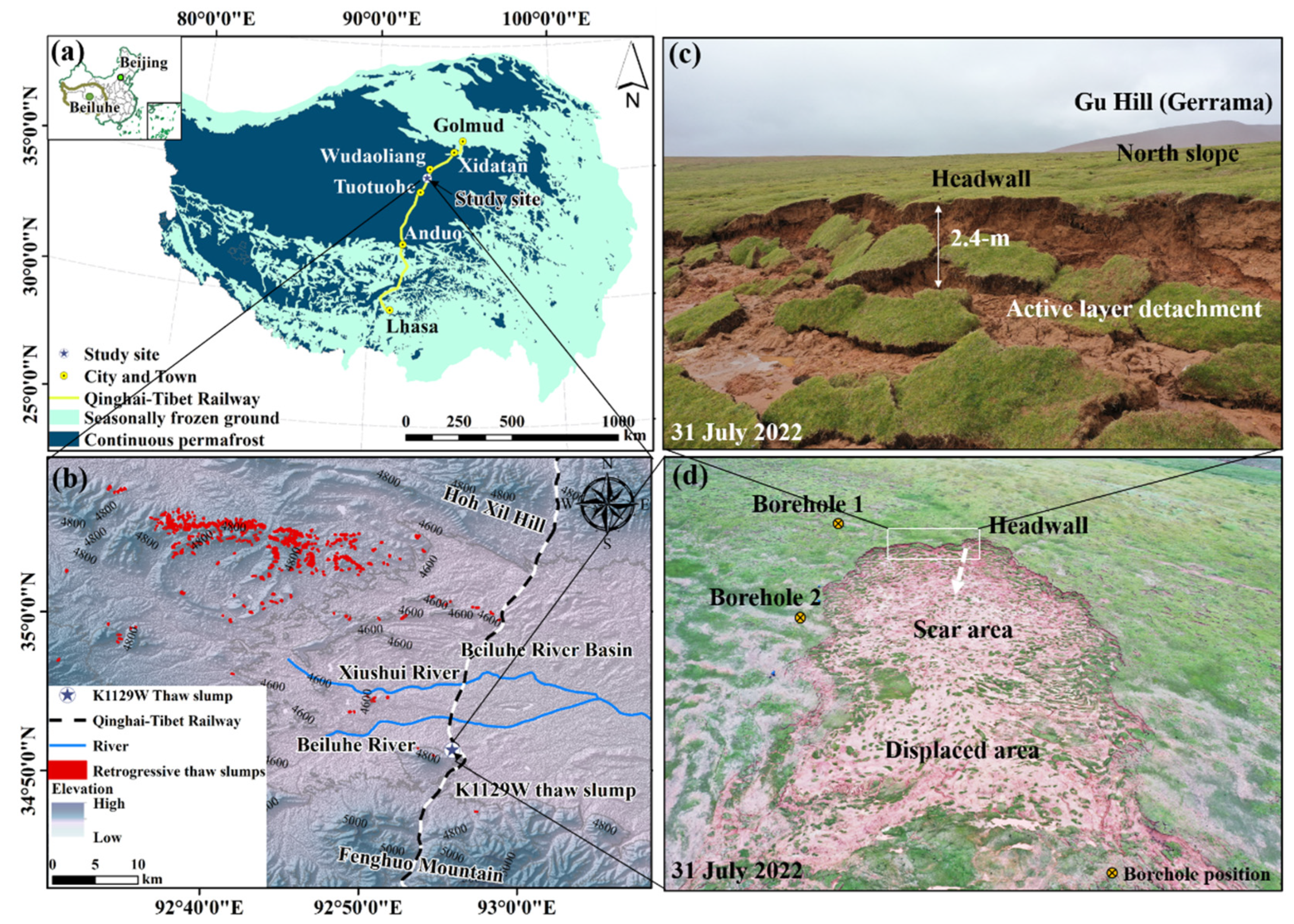
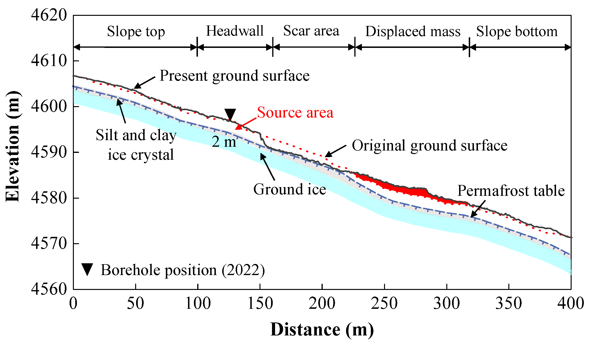
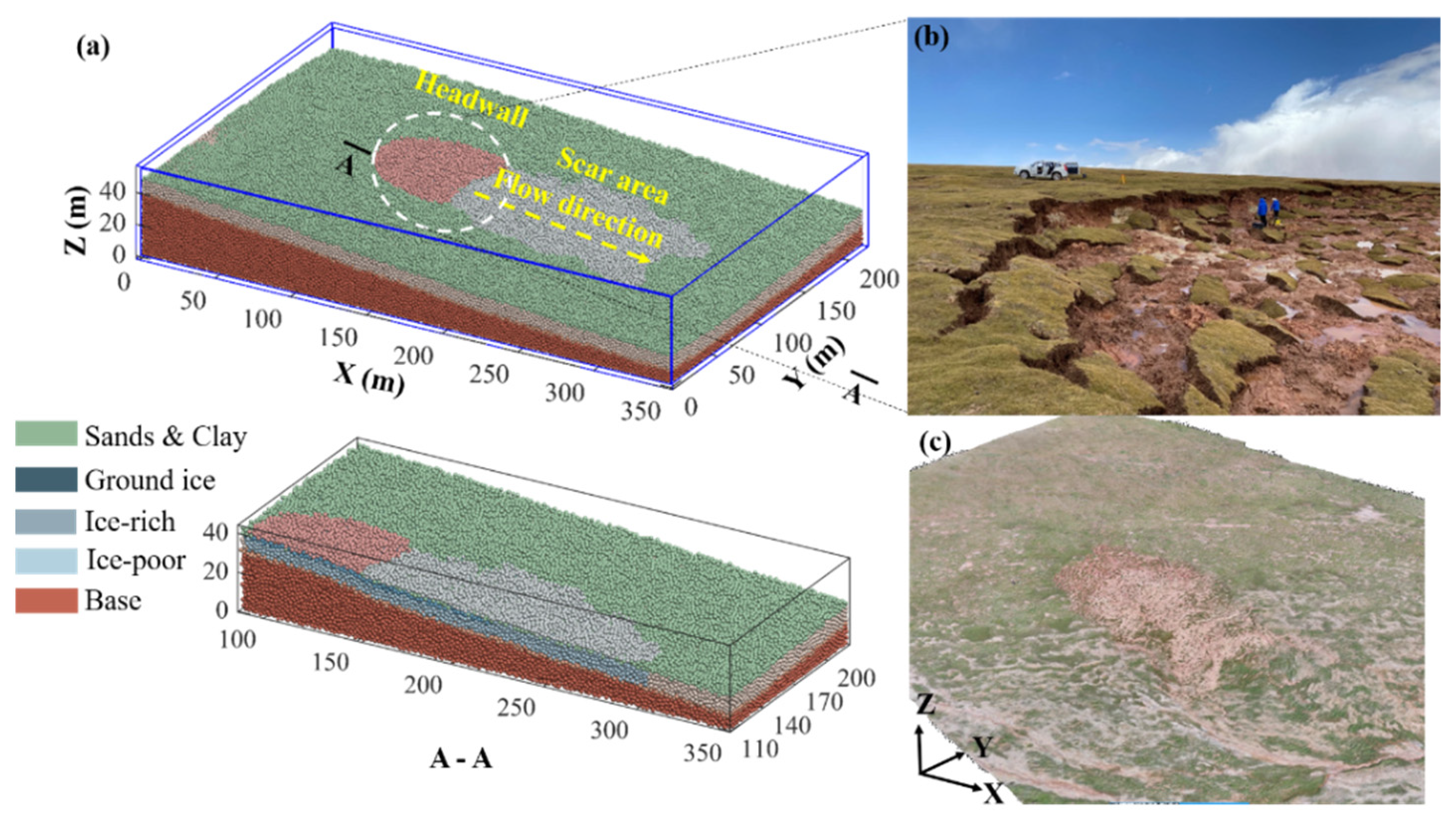
2.1. Study Site Description

The studied thaw slump developed on the west side of the K1129 mileage of the QTR, which is in the Beiluhe River Region—the hinterland of the QTP. The elevation is from 4418 m a.s.l to 5320 m a.s.l, with a mean of 4673 m a.s.l [10]. The mean annual air temperature (MAAT) in this region is −3.8 °C and the mean annual precipitation is more than 300 mm over the period from 1957 to 2020, falling mainly in summer [9,10,25].
Figure 2 shows a two-dimensional sketch of the longitudinal section of the K1129W thaw slump. The present ground surface elevations were investigated through the TLS survey in August 2022, and the original ground surface data were from the ALOS PALSAR in 2010 (https://search.asf.alaska.edu/, accessed on 4 October 2010). The thaw slump development area, with a gentle slope, is between 6.8° and 10°. The current dimensions of the K1129W thaw slump were approximately 155 m in length from the headwall to the compressed area, and 95 m wide in the middle position (the widest position was 112 m). It involved the displaced materials with a volume of 12,160 m3, and the total disturbed area was about 11,268 m2. A 1.4 m to 2.4 m high headwall formed in the west of this thaw slump, and about 8% to 15% of the scar area was mainly covered by alpine meadow (Figure 1).
Based on the core logging information for drilling near the thaw slump development area in 2022, the main formation conditions are shown in Figure 3a. The superficial layer (0.5 m to 1 m in thickness) is fine sands and gravels, with a small amount of root system. The underlying strata are mainly silty clay (the most thickness is up to 8 m) and the substratum is mudstone with sandstone interlayers [26]. The soil in this area is relatively dry and the gravimetric moisture content (ground ice content) was tested in situ. As illustrated in Figure 3b, the moisture content curves can reflect the ground ice content in this area. The permafrost table is 1.95 m deep. The depth of the ground ice layer is approximately 2.2 m to 3.5 m (the natural area), as estimated from the borehole drilling at the southwest of the back scarp. The ice content, near the permafrost table, is 68% to 88% at the depth of 2.2 m to 4 m from the ground surface. Additionally, the mean annual ground temperature (MAGT), at the depth of 10 m, is about −1.52 °C.

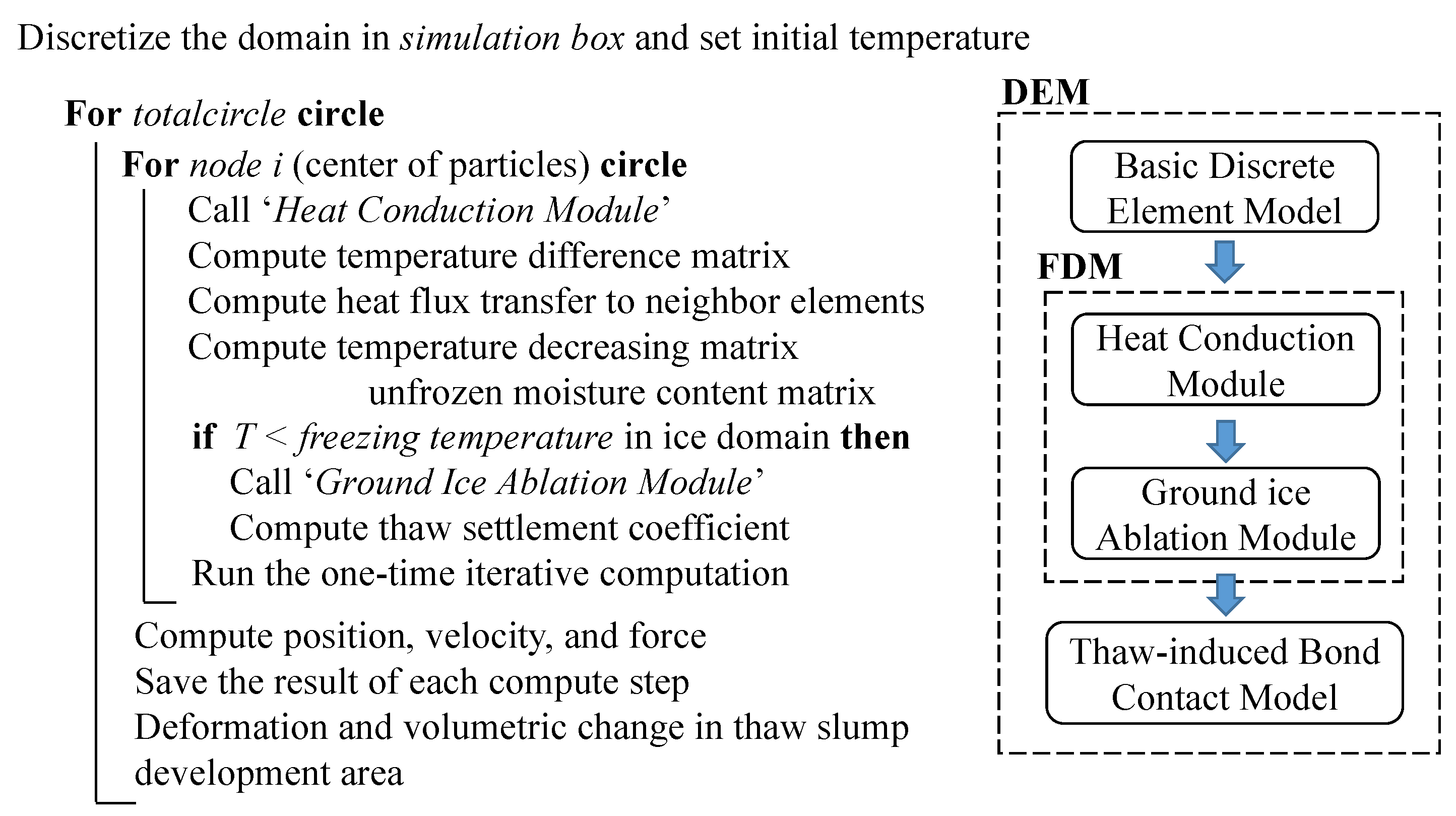
2.2. Computation Module Description

The 3D discrete element thaw slump model was developed in the basic discrete element model frame, and the heat conduction equation and the ground ice ablation computation module were coupled to simulate heat transfer, latent heat, and ground ice melting.

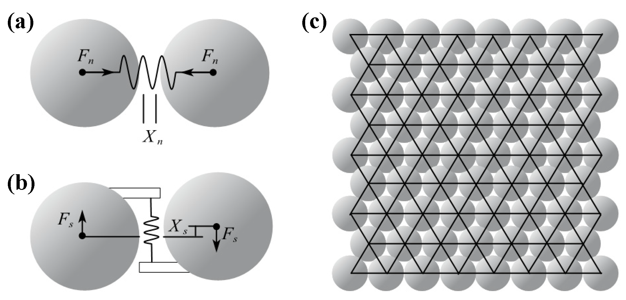
2.2.1. Basic Discrete Element Module

The discrete element method was originally developed for the behavior of the kinds of granular assemblies [27]. Moreover, researchers employed the bonded discrete element model to simulate the behavior of cohesive materials, for instance, clay and rock glacier [28,29,30]. A close-packed lattice solid model was applied to the landslides [30,31,32,33,34].
In this paper, the model is composed of a series of uniform and close-packed elements to represent active layer soil, ground ice, and permafrost (Figure 4). Based on the most basic linear elastic model, the interaction between the elements and their neighbors was bonded or broken by the normal spring force. The inter-element normal spring force (Fn) is defined as the product of relative normal displacement (Xn) and normal contact stiffness (kn). The equation of the normal spring is:
F n = { k n X n , X n < X b ,   intact bond k n X n , X n < 0 ,   broken bond 0 , X n 0 ,   broken bond
where Xb is the breaking displacement.
Similarly, the tangential spring force (Fs) is defined as the product of the shear relative displacement (Xs) and shear stiffness (ks). The equation of the tangential spring is:
F s = k s X s
An intact bond may fail in a tangential direction when the inter-element shear force exceeds the maximum shear force (Fsmax) allowed by the Mohr–Coulomb criterion [28,35].
F s max = F s 0 μ p F n
Figure 4. Diagrammatic draft of the linear elastic model. (a) Two particles interact through a spring force (Fn). (b) Two particles are also bonded by a spring along the tangential direction to simulate the shear force (Fs). (c) A close-packed discrete element model [36].
Remotesensing 14 05592 g004

2.2.2. Heat Conduction Module

Under climatic warming and wetting, the rise in the permafrost temperature causes exposed ground ice ablation. A heat transfer module was developed herein for the calculation of the particle temperature in the discrete element model which represents the ground temperature. Due to the downward ground temperature, the heat (energy) flux QA of element A in the heat conduction can be calculated by Fourier’s law, which is written as:
Q A = λ A | R 1 R 2 | Δ T
where λ is the thermal conductivity (W/m°C = J/m/s/°C); A is the cross-sectional area (m2) of the heat flow which is defined as the contact area between element A and its neighboring elements; |R1R2| is the distance between element A and its neighboring elements; and ΔT is the temperature difference between element A and its neighboring elements. As the heat conduction is performed in a porous medium, the thermal retardation R was introduced into this process. The relationship between the thermal retardation R and the temperature difference ΔT is represented by the following equation:
Δ T n i = R l q i
where ni is the direction vector; l is the distance of the heat transport; and qi is the heat flux on the unit length.
Based on the apparent heat capacity method [37], the ice–water phase transition latent heat was considered in the model. The latent heat QH in the porous medium is approximated by Equation (6). Additionally, it can change the element temperature, which is defined by Equation (7)
Q H = θ ρ i L Δ W u ( T )
δ T = Q H / m c
W u ( T ) = ( 1 p ) e ( T / q ) 2 + p
where θ is the porosity; ρi is the density of ground ice (kg/m3); L is the latent heat of thawing (J/kg); δT is the temperature difference of the element; m is the mass of an element (kg); c is the specific heat of an element (J/kg/K); and Wu(T) is the temperature-dependent function of unfrozen water content (see Equation (8)), which relates the unfrozen soil moisture to the soil temperature. The experimental constants p and q are related to soil properties [38].

2.2.3. Ground Ice Ablation Module

Thaw settlement is the process of soil skeleton compression and drainage consolidation. It is mainly reflected in the ground surface settlement caused by permafrost thawing or ground ice ablation, consisting of the ice–water phase-change deformation and compression deformation under an external load [39]. In terms of the retrogressive thaw slump (RTS) development area, there was no external load on the slope surface of our study site. Moreover, the consolidation process due to the rearrangement of elements and changes in pore structure can be considered in the discrete element model. The thaw settlement is calculated at each step according to the volumetric change in the moisture content of the elements. The governing equation of vertical deformation (frost heave/thaw settlement) can be defined as [40,41]:
S = θ S w Δ W u ( ρ w ρ i ρ i ) ( H 2 H 1 )
where S is the vertical deformation (m) over the computing time step; θ is the porosity; Sw is the water saturation; ΔWu is the volumetric change in the unfrozen water content over the computing time step; ρ is the density (kg/m3); and the subscripts w, and i represent water and ice, respectively. Additionally, H1 and H2 are the original thicknesses of the permafrost before and after thawing or freezing. Simultaneously, the dimension of elements will be smaller when considering ground ice ablation. A simple thawing- or freezing-induced variation in particles can be expressed as:
R k + 1 = α t R k
where R is the radius (m) of the element and the subscripts k and k + 1 represent the computing time step. Additionally, the deformation coefficient αt is calculated by the above-mentioned process. Equation (10) can be used to solve the thaw settlement problem. Because the whole process of thermokarst subsidence cannot be completed in the RTS development area, thawed materials slide down to the slump floor. It is necessary to improve the contact model for the research of RTS development.

2.2.4. Thaw-Induced Bond Contact Model

For cemented granular materials, such as icy permafrost, elements are bonded together through the cementation of the pore ice or segregated ice in the soil. Such intergranular cementation is susceptible to thaw-induced change. Especially for ice-rich permafrost, ground ice ablation can cause the shrinkage of icy particles and a reduction in shear strength-related parameters. Such an “ice-melting” process can be realized via an apt definition of contact models [42,43,44]. For feasibility and generalization, we introduce a “weakening or melting” coefficient αw into the basic contact model that governs the thawing-induced cementation breakage. The normal and tangential force of the weakening contact model is calculated by:
F n > α w k n X n ,   X n | R 1 R 2 | broken bond
F s > μ w F n b , F n b = α w k n | R 1 R 2 |
where αw represents the “weakening or melting” coefficient in connection with the normal contact stiffness kn; |R1R2| represents the center distance of the two contacting elements; and μw represents a threshold of μp, which is the coefficient of maximum shear force corresponding to the normal broken force in a thawing state and assumed independent of temperature. The normal spring force is becoming weak and cannot sustain enough tension. The “weakening or melting” coefficient αw is affected by several parameters including temperature, soil type, and water chemistry. The weakening coefficient αw is defined as a function of the unfrozen moisture equation, which is a temperature-dependent coefficient. Note that the function of the weakening coefficient is used for the thawing phase.
α w = { A ( W u ( T ) W u ( T t ) ) , T < T t 0                                                                     , T T t
A = θ S w ( ρ w ρ i ) / ρ i
where A is the soil texture-related coefficient, which can be estimated by Equation (14); Tt is the melting temperature of permafrost. Both A and Tt in this study are assumed to be constant.

2.3. Setup of Model and Parameters

Ground ice ablation induces permafrost thaw-related consolidation problems widely found on the QTP, such as thermokarst subsidence, thermal erosion, thermokarst lake, and thermokarst landslide. To solve this kind of large deformation problem, a discrete element method software MatDEM [45] was employed in this study. Through the secondary development, an improved bond contact model considering heat transport, ice–water phase change, and thaw settlement consolidation was used in the simulation. The numerical simulation is mainly carried out from the following two parts: (1) the shear behavior in the basal zone of the active layer; (2) deformation and volumetric change in thaw slump development.

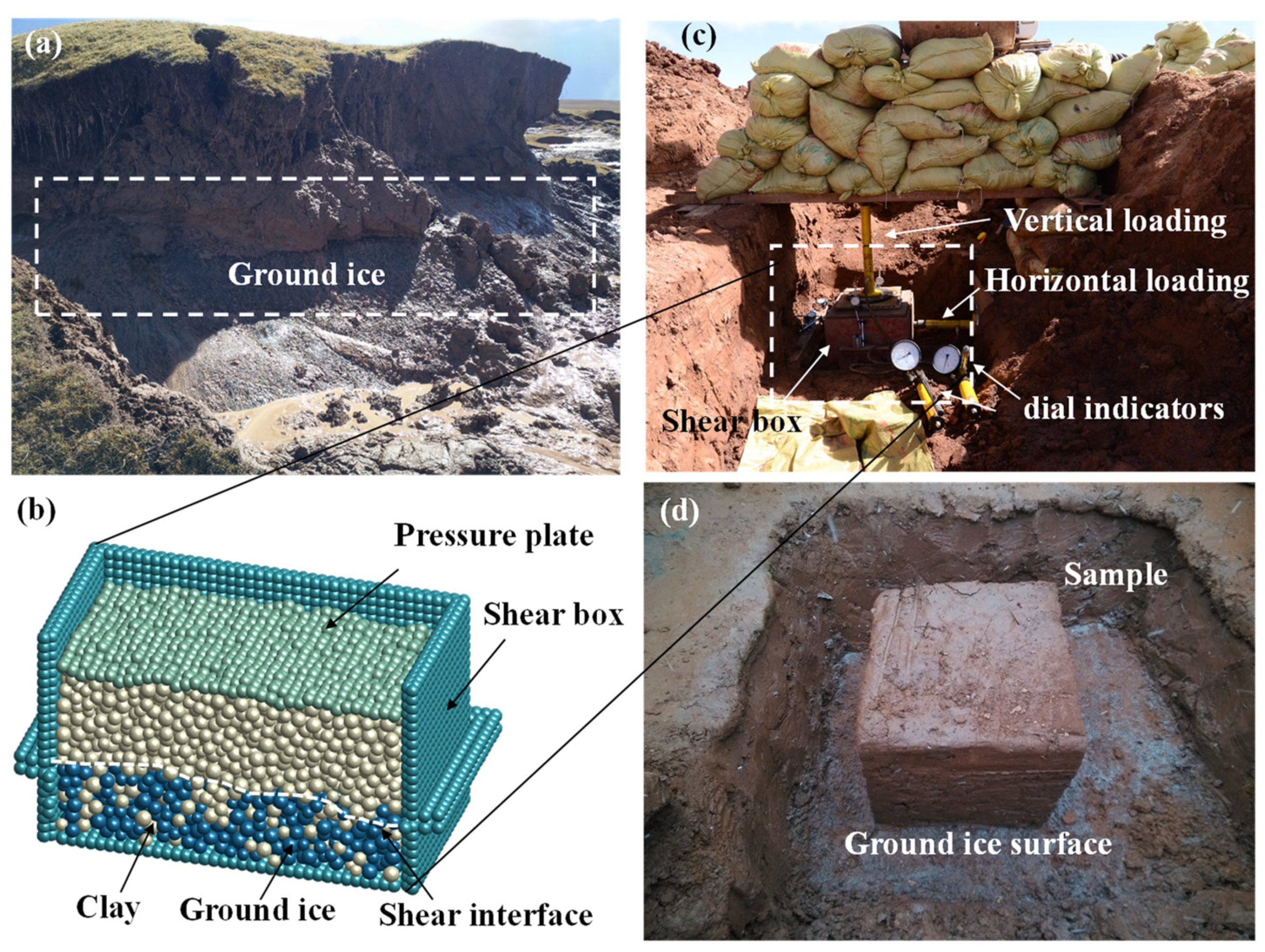
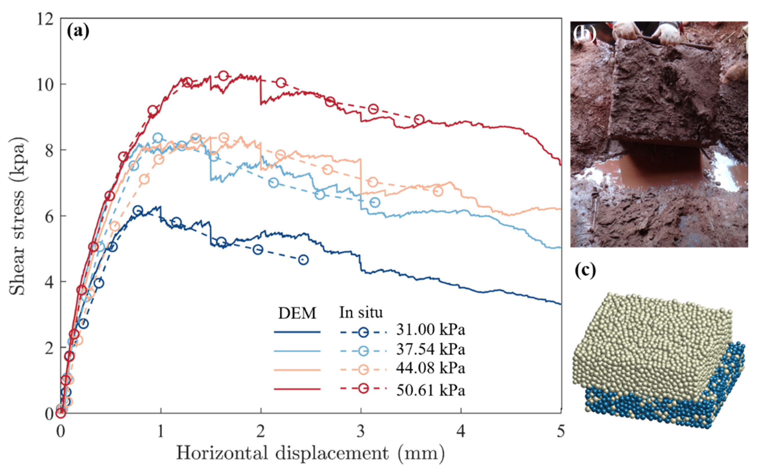
2.3.1. Basal Zone Shear Test Model

To understand the shear behavior in the basal zone of the active layer, especially for the permafrost thaw state, a DEM simulation of a direct shear test was first conducted in this work concerning the in situ shear tests [9] near this study area (the specific direct shear test apparatus is shown in Figure 5). Two sets of in situ shear tests were executed at a gentle slope site near the previously studied landslides on the Beiluhe River Basin [9]. Each set of experiments loaded four groups of vertical pressure from 1 to 1.6 times of gravity pressure on the top plate because excessive vertical pressure causes a change in strength parameters between the sample and ground ice.
Figure 5 shows the experiment setups of the simulation and in situ tests. The specimen was discretized into 23,500 elements in the model and the radius of each particle was from 1 to 1.414 mm. A 50 mm by 50 mm by 30 mm specimen was placed in the same inside size shear box (generated by the cluster elements in MatDEM), and the vertical stresses of 31.00, 37.54, 44.08, and 50.61 kPa were applied to the top plate. The simulation adopted the horizontal displacement load to the sample. The total displacement was 5 mm, which was decomposed into several loading steps (each step was 0.25 mm), and each cyclic step was broken into 2500 steps. In addition, the volumetric ice content at the active layer–ground ice interface was assumed to be 46%, which was from the borehole data.
Moreover, three weakening coefficients αw were used to prepare the different thawing states of ice-rich permafrost. To reveal a preliminary law on the shear strength parameter “weakening” in the interface between the active layer and the ground ice, three scenarios of the inter-granular cementation weakening coefficient αw were executed with 0.03, 0.01, 0, where the selected vertical pressures were consistent with the aforemetioned direct shear test. The geotechnical parameters of each material are listed in Table 1.

2.3.2. Thaw-Induced Slope Failure Model
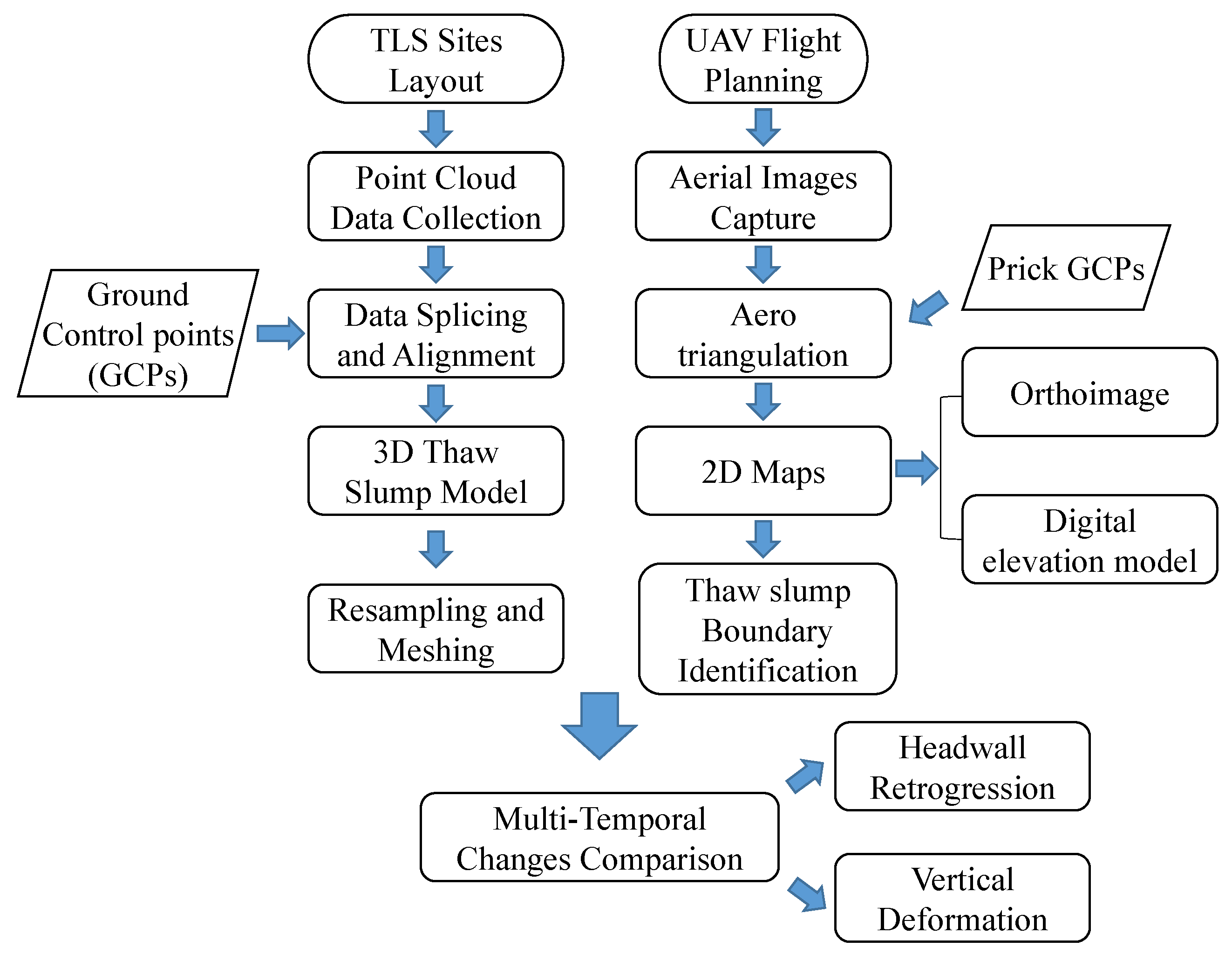
To quantitatively assess the deformation and volumetric change in RTS, a simulation of a typical thaw slump development process was performed, and the dynamic of the sliding particles from the source area was recorded. The massive ground ice ablation contributed to the reduction in the shear strength in the basal zone and the active layer particle instability. The moving elements represented the solifluction materials that slid and flowed. Concurrently, a steep back scarp was formed on this gentle slope. Based on this kind of thermokarst landslide’s typical characteristics, a three-dimensional discrete element model of the K1129W thaw slump was used, as shown in Figure 6. The deposited elements were molded according to the digital elevation model and placed in a rectangular simulation box [36] (integrated into the MatDEM). The numerical model consisted of 5 layers from the ground surface to the bedrock and was 350 m on the X-axis, 220 m on the Y-axis, and 0 to 48 m on the Z-axis (Figure 6). We built this thaw slump model with 224,388 active elements and 252,003 wall elements using discrete particles with an average radius of 1 m. The physical properties are listed in Table 2.
The flow chart (Figure 7) illustrates the specific implementation processes of coupling the aforementioned computation modules in this discrete element model. The detailed simulation procedure is described in the following steps. Firstly, based on the finite difference method (FDM), we generated the temperature differences matrix of the thermal disturbance elements and their neighboring elements. Additionally, the heat flux was then calculated for these elements. Concurrently, the element temperature was recorded in the “d.mo.SET. aT” matrix. Secondly, the unfrozen moisture function was used to calculate the change in unfrozen water content under the temperature condition in this step. Furthermore, the dimension of the particles was adjusted by integrating their equations of thawing vertical deformation when the element temperature was greater than 0 °C. Simultaneously, the program calculated the elements’ temperature reduction due to the release of phase change latent heat and recorded the final temperature of an iterative calculation step. At the same time, the shear strength in the basal zone was detected and the friction-related parameters of the interface between ground ice and the basal zone were adjusted in the thaw-induced bond contact model. Lastly, the particles were advanced to new positions under gravity conditions in the Newtonian physics system. The simulation was run for 1000 steps until the neighbor elements became positive.

2.4. TLS-UAV Method

To calibrate the simulation results, a combined method of terrestrial laser scanning (TLS) and unmanned aerial vehicle (UAV) was put forward. The details of the data acquisition and processing are as follows.

2.4.1. Terrestrial Laser Scanner Survey

To obtain a high-resolution point cloud of the K1129W thaw slump development area, the Leica P50 terrestrial laser scanner was employed in our study. The picture acquisition speed is up to 976 k points/s, and the maximum scanning distance is 120 m. The scanning scope was set from −55° to 90° in the vertical direction and 0° to 360° in the horizontal direction, and the scanning accuracy was set as 1.6 mm of a 10 m scan radius. To measure the total volumetric change and deformation in the thaw slump development area, two TLS investigations were performed in September 2021 and August 2022. Each scanning contained 8 stations.
The post-processing software Leica Cyclone 9.2.0 (https://leica-geosystems.com) was used for the massive point cloud data splicing of adjacent station data and the coordinate system conversion. After basic preprocessing, spatial sampling was conducted and the unrelated points were removed. Additionally, the 0.1 m spacing points were then extracted and were meshed to the time series triangular irregular networks (TINs). Furthermore, the TIN comparison work was executed in Matlab 2019b.

2.4.2. Unmanned Aerial Vehicle Survey

To supplementarily quantify the thaw slump deformation and volumetric change, the UAV-based orthoimages and digital elevation model of the investigated thaw slump were utilized to reconstruct the 3D model and digitalize the K1129W thaw slump area. DJI Matrice M300 RTK, equipped with a Zenmuse P1 visible light camera lens, was employed to take aerial photos of the K1129W thaw slump and the surrounding area. DJI Pilot 2 software was used to plan the flight route and control the aircraft. The flight height was set to 60 m higher than the headwall, and the overlap rate was set at 75% in the heading direction and 85% in the sidewise direction. Two UAV fights were conducted in September 2021 and August 2022. Eventually, the aerial images of every fight were imported into the post-processing software DJI Terra to conduct aero-triangulation and model reconstruction. Additionally, high-resolution (<10 mm) orthoimages and the 3D model presented detailed information on the K1129W thaw slump. The comparative analysis can replenish the TLS investigation. Figure 8 shows the overall analysis flow chart of the TLS-UAV method.

3. Results

3.1. Shear Strength of the Ground Ice and Active Layer

This study first obtained the shear stress–displacement relationship of the basal zone in the detachment failure process between the active layer and the ground ice layer (Figure 9). It is evident that an obvious stress-softening process is presented in the shear stress–displacement curves. Concurrently, the shear stress and horizontal displacement curves of the discrete element model were demonstrated by the authors’ previous in situ test [9]. Figure 9 also illustrates a good consistency between the model and the field experiment.
Figure 10 shows the evolution of the shear stress displacement with different interface strength parameters of the weakening coefficient αw for the specified loading plate. It is clear that both the peak and residual shear stresses decrease with the cementation weakening coefficient αw for one given vertical pressure. With the decline in the granular cementation weakening coefficient αw, the appearance of stress softening was not obvious. Moreover, with the peak shear stress decline due to the friction coefficient decrease, granular cementation is more liable to break. Thereby, the critical stress was approaching the low-cementation weakening coefficient scenario. In addition to determining the strength parameters in the basal zone of the active layer, the direct shear test simulation can, in turn, demonstrate granular cementation “weakening or breaking” due to the ground ice ablation module described in Section 2.3.2.

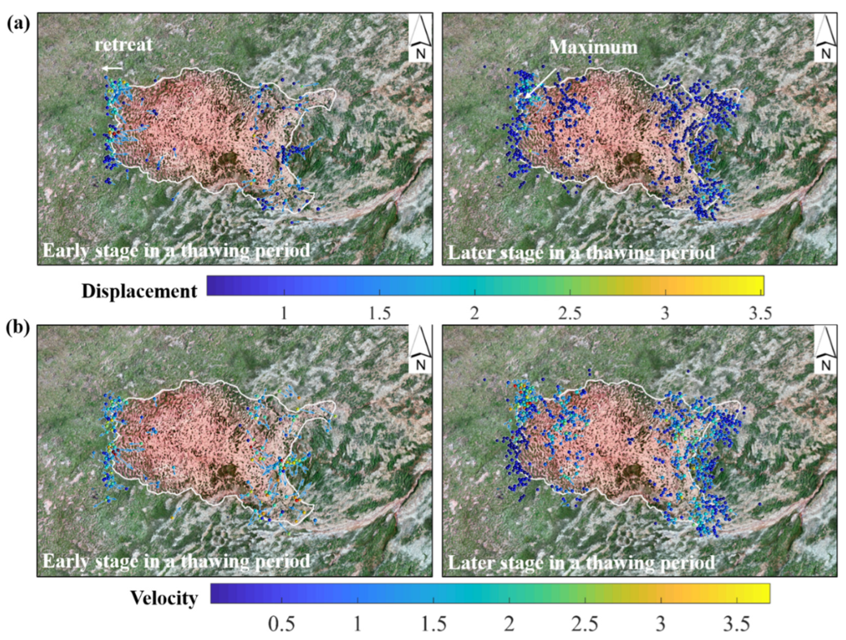
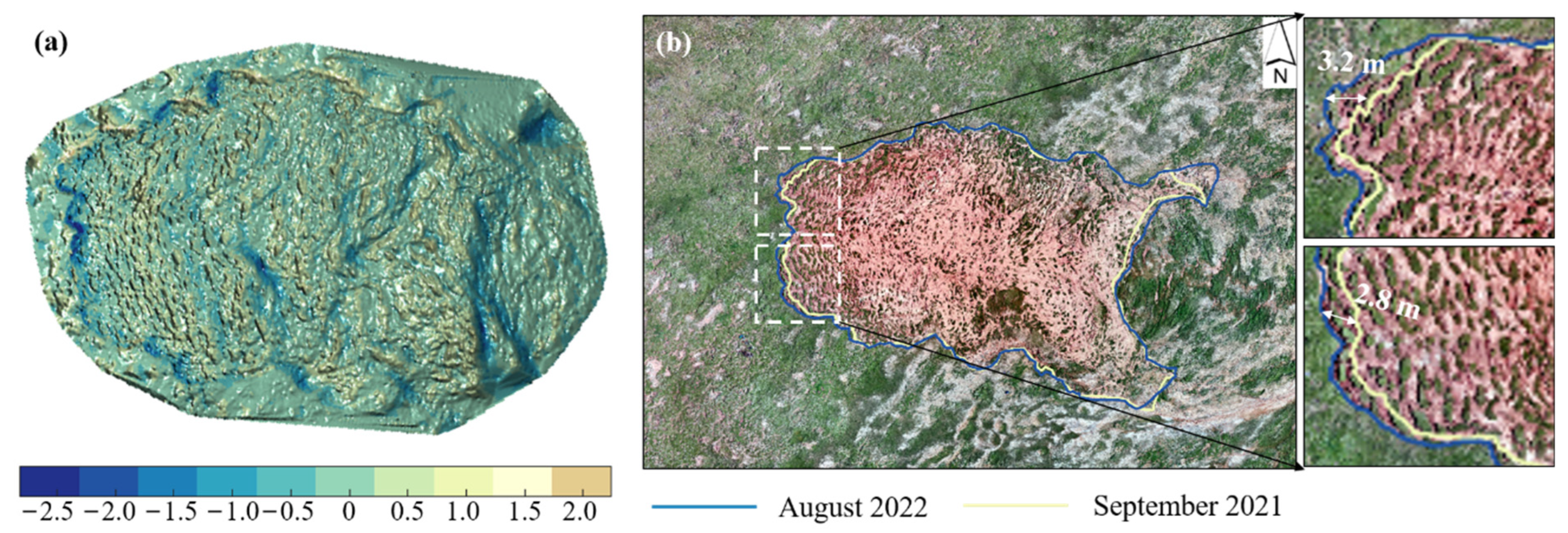
3.2. Deformation and Volumetric Change Analysis

Heat conduction in ice-rich permafrost can impact the granular structure, shown as shear strength decreases through the thaw-induced contraction of particles and weakening of the cementation between the particles. It is, therefore, indispensable to demonstrate the deformation characteristics of RTS under climatic warming. Due to climatic warming and wetting, the exposed ground ice at the lower part of the headwall was beginning to melt. Furthermore, the cementation of thawing elements was gradually weakening.
Figure 11 shows the deformation simulation results of the K1129W thaw slump to elucidate and present concise results, and the resultant displacement of particles with more than 0.5 m is extracted from the model. For conciseness, these extracted elements are superimposed on the image of the K1129W thaw slump area. The white boundary line represents the thaw slump development area outlined from the orthoimage of the UAV survey in September 2021 (Figure 11). Concurrently, the subsidence and headwall retrogression (Figure 11a) and sliding direction velocity component (Figure 11b) in the thaw slump development area were also calculated in the model. During the one-time thaw slump process, the overall vertical deformation varied dramatically in the lower part of the headwall, with subtle variations in collapsed scar area; following the active layer detachment failure at the headwall, the thawed particles slid down the sliding surface and flowed to the front edge of the slope. The ground subsidence reached 2.3 m at the lower part of the headwall. Figure 11a shows the headwall retreat of the K1129W thaw slump. The total displacement of headwall retrogression was approximately 2.2 m to 3.5 m during a one-time thaw slump process. Especially for the northwestern part, the retreat distance reached 3.5 m, and this is the location where the maximum ground subsidence occurred. Figure 11b shows the velocity evolution of melting or sliding mass. At the active layer detachment failure stage, the velocity of the thawed materials increased dramatically. Additionally, the maximum velocity of particles was 3.1 m/s. After the detachment failure, the velocity of most elements declined and gradually stopped at the front edge of the thaw slump development area. Most particles at the front edge of the sliding mass did not have an evident velocity at the end of the computation time. The potential energy of RTS caused by the ground ice ablation at the lower part of the headwall may have dissipated. Note that the simulated headwall retrogression retreated evenly due to the ground ice content, and distribution was assumed to obey uniform distribution. However, we could not obtain the ground ice distribution of the entire thaw slump development area, which was limited by geological data and field harsh conditions. The comparison between the annual change in the thaw slump boundary lines and the simulation results is introduced in Section 3.3.
To quantitatively estimate the volumetric change in the K1129W thaw slump, the dynamic of the sliding particles from the source area was recorded. As illustrated in Figure 11, about 437 elements slid from the source area to the collapsed scar area. Less than 125 particles slid out of the trailing edge of the landslide, which presented the soil erosion or mass wasting of the RTS. During this one-time thaw slump process, the mass wasting that occurred in the lower part of the headwall was approximately 1335 m3, the volumetric change in displaced mass in the thaw slump development area was approximately 1050 m3, and the volume of the soil erosion was approximately 211 m3.

3.3. Comparisons between Geophysical Survey and Simulation

To quantify the deformation and volumetric change in the K1129W thaw slump and verify the simulation results, this research delineated the thaw slump development area margin using a high-resolution digital elevation model and a TIN model for 2021 and 2022. The blue and light yellow lines represented the boundary of the K1129W thaw slump in September 2021 and August 2022, respectively (Figure 12b). The negative values in Figure 12a indicated the erosion or thaw settlement zone of the thaw slump development area, representing the ground subsidence due to the melted or collapsed materials sliding to the deposition zones. On the contrary, the positive values indicated the displaced area, denoting the accumulation of deposited materials from the thawed headwall. Through the superposition analysis of these data, the calculated vertical deformation and headwall retreat results were shown in Figure 12 between 2021 and 2022. The significant deformation of the headwall retrogression and surface subsidence appeared in the northwest of the thaw slump development area. During this period, the headwall retreat values in the southwestern and northwestern “lobe” parts were approximately 2.8 m and 3.2 m, respectively. Additionally, the vertical deformation was −1.9 m at the lower part of the headwall. The geophysical investigation and simulation results were in good agreement. In addition to the good consistency of the deformation, the TLS and UAV survey results can display the deformation characteristic more delicately. Especially for the thaw slump retrogression, the results can indirectly reflect the ground ice ablation.
To calculate the volumetric change in the thaw slump development area, the time series of the high-density point cloud from the TLS survey was conducted for comparison. The retreat of the headwall caused an increment in the collapsed scar area. With the thawed materials sliding down the face of the headwall, most of the materials were left in the displaced area and the others flowed away. The total volumetric change was about 1412 m3 in the thaw slump development area. Among them, about 1124 m3 was added to the displaced area. Thus, the estimated amount of mass wasting was about 288 m3.

4. Discussion

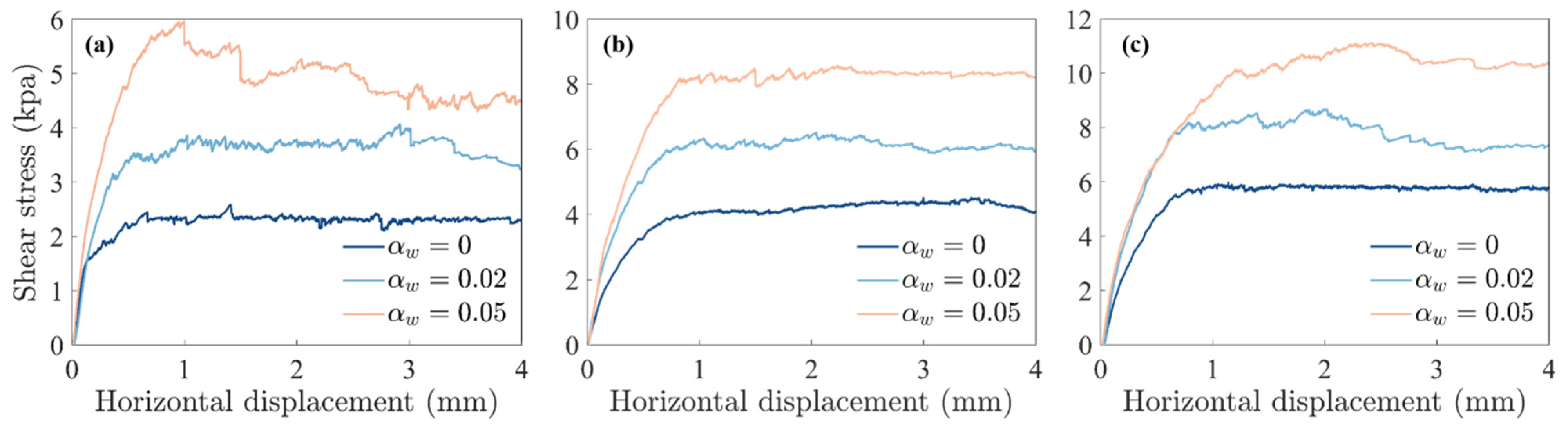
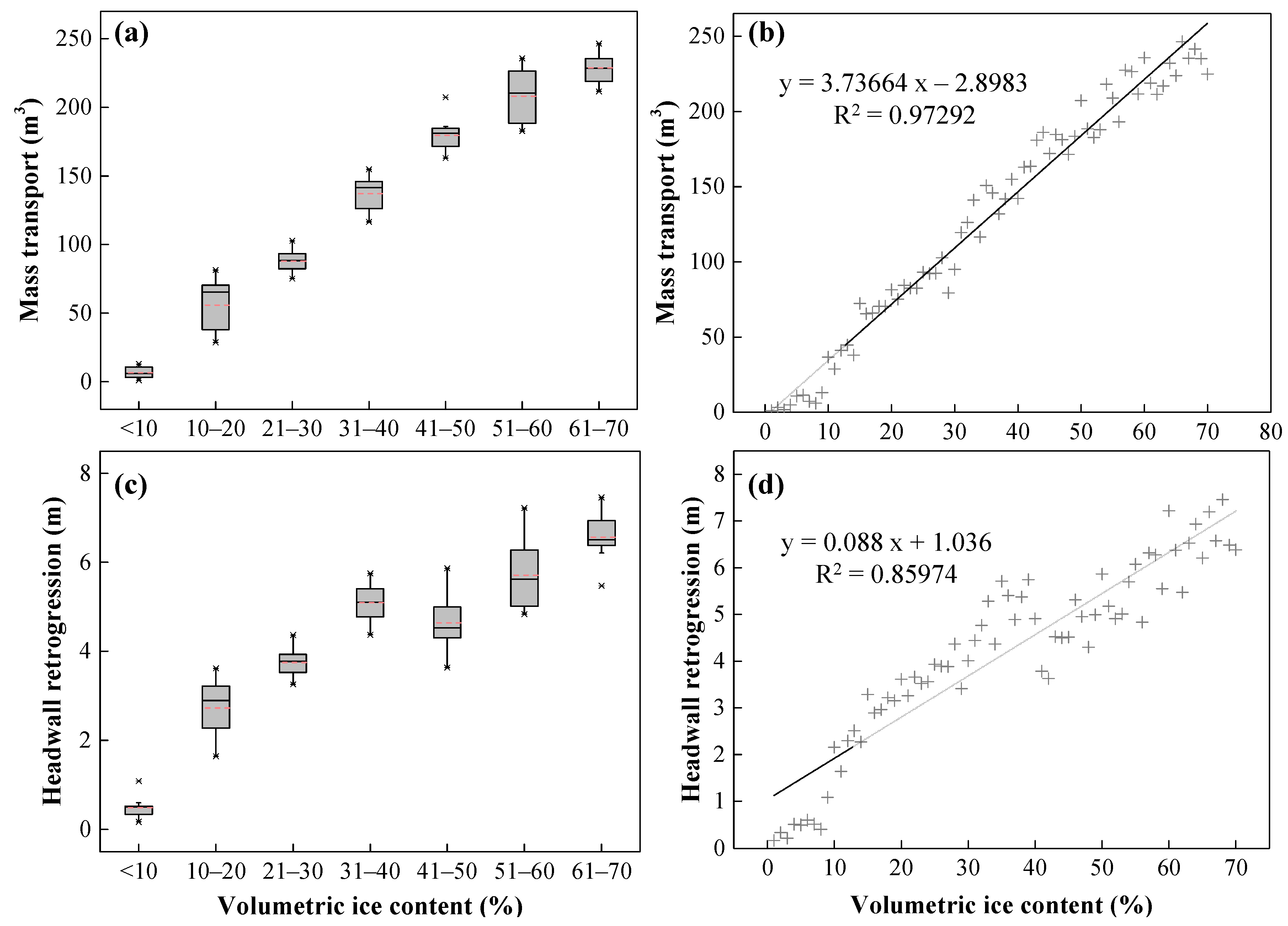
4.1. Impact of the Ground Ice Content

Ice-rich permafrost thawing, or massive ground ice ablation, are the most significant prerequisites for RTS development. Ice-rich permafrost in the study area comprises pore ice, segregated ice, soil mass, unfrozen water, and gas-filled voids [46]. In a natural state, during the one-sided thawing of the active layer in a warm period, unfrozen water migrates downward toward the thawing front descending from the ground surface when there are a negative ground temperature gradient conditions [47]. However, in the RTS development area, the headwall of RTS showed exposed ground ice, especially in our study site. Under high air temperature and heavy rain conditions, the rate of ground ice ablation increased, and the meltwater seeped or drained to the sliding face. Due to the ground ice melt, the shear strength of soil near the permafrost table would decrease and the pore water pressure would increase simultaneously.
Therefore, the ground ice content can affect the intergranular cementation state in permafrost. In this study, the thaw slump development process was simulated with different volumetric ice contents (from 1% to 90%). Due to the headwall retrogression being highly related to the height of the headwall, the slope angle, and the scale of RTS [48], this study quantitatively estimated the mass wasting and headwall retrogression in a determined headwall height and thaw slump scale. Thus, the ratio of the retrogression and height in the frozen back scarp was defined as retrogression ratio r1, and the ratio of the volumetric change and thaw slump development area was defined as mass wasting ratio r2. Figure 13 presents that the mass wasting and headwall retrogression tended to enlarge with the increase in ground ice content. The minimum volumetric ice content of active layer detachment failure was about 10% in this thaw slump. The volumetric change and headwall retrogression increased approximately linearly (r2 = 0.9729, p < 0.001, n = 70; r2 = 0.8597, p < 0.001, n = 70, respectively) with volumetric ice content in this study site. With a higher ground ice content, the bonds were more susceptible to “weak or breakage”, and thereby the elements in the active layer group were prone to slide.

4.2. Research Deficiencies

Although the fast GPU-based discrete element method (DEM) is a high-efficiency means to calculate large deformation problems, the thermokarst landslide is a long-term evolutionary process that is different from traditional landslides, such as avalanche and debris flow. The mud-flow materials in the scar area make it difficult to drill in RTS development areas. We could not obtain the ground ice content in the scar area. Thus, the model mainly simulated the active layer detachment failure at the steep frozen back scarp and the thawed materials downslope sliding during the thawing season. Moreover, the simulation did not consider the solifluction that remained on the scar area after the last thawing season. The difference between the simulation and TLS-UAV is mainly owing to this reason. Additionally, the TLS-UAV method can acquire a set of high-density three-dimensional point cloud coordinates of RTS. Investigation data can be utilized to build a detailed geomorphological picture and analyze the deformation [23]. However, this is limited by the accessibility of the study area because most RTSs are located in no man’s land. Concurrently, a high-resolution digital surface (elevation) model is needed for an accurate real terrain numerical model. Furthermore, there is the limitation that the remoting sensing method cannot accurately assess the order of mass wasting less than 500 m2 and elevation changes less than 1.6 m [8].
To replenish the limitations of the remote sensing and TLS-UAV combined methods, as well as to meet ordinary computer computing, it is essential to simulate these “small-scale” thaw slumps in the QTP. Meanwhile, the method presented in this paper can be used to estimate the evolution of landslides, especially for mass wasting and headwall retrogression.

5. Conclusions

In this research, we quantitatively assessed the seasonal deformation and volumetric change in a typical thaw slump in the permafrost terrain of the QTP with a discrete element model and geophysical model. We found that the results of ground subsidence, mass wasting, and headwall retrogression were well described by the simulation. Some valuable findings were drawn as follows:
(1) We proposed a systematic computation procedure, GPU-based DEM-FDM, for the effective simulation of the coupled thermo-mechanical thaw-induced slope failure problem. It is demonstrated that the thaw-induced bond contact model can effectively present the “weakening” of intergranular cementation, showing the shear strength decrease. Concurrently, the law of shear strength in the basal zone of the active layer under the thawing or thawed state was determined by the simulation.
(2) In a thawing season, the total volumetric change was approximately 1335 m3. Headwall retrogression was about 2.2 m to 3.5 m and the surface subsidence reached 2.3 m in the lower part of the headwall. Approximately 1050 m3 of thawed materials were moved to the displaced area, and the amount of soil erosion was about 211 m3.
(3) The minimum volumetric ice content required to trigger active layer detachment failure is approximately 10%. The relation between volumetric ice content and mass wasting can be expressed as a linear equation.
TLS-UAV technology and the DEM-FDM method can replenish the limitations of remote sensing, especially for “small-scale” RTSs. This kind of behavior, especially for the impact of ground ice content, can provide valuable insights into predicting the future RTS evolution of the QTP and the Arctic. Additionally, quantifying soil erosion has significant implications for the assessment of the eco-environment of the whole QTP.

Author Contributions

Conceptualization, F.N., C.J. and J.L.; methodology, C.J.; software, C.J. and P.H.; validation, L.R., Y.S. and J.L.; formal analysis, C.J.; investigation, F.N., C.J. and P.H.; resources, F.N. and J.L.; data curation, C.J., L.R., Y.S. and P.H.; writing—original draft preparation, C.J.; writing—review and editing, F.N., C.J., Y.S. and J.L.; visualization, C.J.; supervision, F.N., J.L. and Y.S.; project administration, F.N.; funding acquisition, F.N. All authors have read and agreed to the published version of the manuscript.

Funding

This work was supported by the Second Tibetan Plateau Scientific Expedition and Research (STEP) Program (Grant No. 2019QZKK0905), the Strategic Priority Research Program of the Chinese Academy of Sciences (Grant No. XDA19070504), and the Guangdong Provincial Key Laboratory of Modern Civil Engineering Technology (2021B1212040003).

Conflicts of Interest

The authors declare no conflict of interest.

References

  1. Zhao, L.; Ping, C.L.; Yang, D.; Cheng, G.; Ding, Y.; Liu, S. Changes of Climate and Seasonally Frozen Ground over the Past 30 Years in Qinghai–Xizang (Tibetan) Plateau, China. Glob. Planet. Change 2004, 43, 19–31. [Google Scholar] [CrossRef]
  2. Ran, Y.; Li, X.; Cheng, G. Climate Warming over the Past Half Century Has Led to Thermal Degradation of Permafrost on the Qinghai–Tibet Plateau. Cryosphere 2018, 12, 595–608. [Google Scholar] [CrossRef] [Green Version]
  3. Schuur, E.A.G.; McGuire, A.D.; Schädel, C.; Grosse, G.; Harden, J.W.; Hayes, D.J.; Hugelius, G.; Koven, C.D.; Kuhry, P.; Lawrence, D.M.; et al. Climate Change and the Permafrost Carbon Feedback. Nature 2015, 520, 171–179. [Google Scholar] [CrossRef] [PubMed]
  4. Lewkowicz, A.G.; Way, R.G. Extremes of Summer Climate Trigger Thousands of Thermokarst Landslides in a High Arctic Environment. Nat. Commun. 2019, 10, 1329. [Google Scholar] [CrossRef] [Green Version]
  5. Farquharson, L.M.; Romanovsky, V.E.; Cable, W.L.; Walker, D.A.; Kokelj, S.V.; Nicolsky, D. Climate Change Drives Widespread and Rapid Thermokarst Development in Very Cold Permafrost in the Canadian High Arctic. Geophys. Res. Lett. 2019, 46, 6681–6689. [Google Scholar] [CrossRef] [Green Version]
  6. Olefeldt, D.; Goswami, S.; Grosse, G.; Hayes, D.; Hugelius, G.; Kuhry, P.; Mcguire, A.D.; Romanovsky, V.E.; Sannel, A.B.K.; Schuur, E.A.G.; et al. Circumpolar Distribution and Carbon Storage of Thermokarst Landscapes. Nat. Commun. 2016, 7, 13043. [Google Scholar] [CrossRef] [Green Version]
  7. Luo, J.; Niu, F.; Lin, Z.; Liu, M.; Yin, G.; Gao, Z. Abrupt Increase in Thermokarst Lakes on the Central Tibetan Plateau over the Last 50 Years. Catena 2022, 217, 106497. [Google Scholar] [CrossRef]
  8. Bernhard, P.; Zwieback, S.; Bergner, N.; Hajnsek, I. Assessing Volumetric Change Distributions and Scaling Relations of Retrogressive Thaw Slumps across the Arctic. Cryosphere 2022, 16, 1–15. [Google Scholar] [CrossRef]
  9. Niu, F.; Luo, J.; Lin, Z.; Fang, J.; Liu, M. Thaw-Induced Slope Failures and Stability Analyses in Permafrost Regions of the Qinghai-Tibet Plateau, China. Landslides 2016, 13, 55–65. [Google Scholar] [CrossRef]
  10. Luo, J.; Niu, F.; Lin, Z.; Liu, M.; Yin, G. Recent Acceleration of Thaw Slumping in Permafrost Terrain of Qinghai-Tibet Plateau: An Example from the Beiluhe Region. Geomorphology 2019, 341, 79–85. [Google Scholar] [CrossRef]
  11. Kokelj, S.; Kokoszka, J.; van der Sluijs, J.; Rudy, A.; Tunnicliffe, J.; Shakil, S.; Tank, S.; Zolkos, S. Thaw-Driven Mass Wasting Couples Slopes with Downstream Systems, and Effects Propagate through Arctic Drainage Networks. Cryosphere 2020, 15, 3059–3081. [Google Scholar] [CrossRef]
  12. Ramage, J.L.; Irrgang, A.M.; Morgenstern, A.; Lantuit, H. Increasing Coastal Slump Activity Impacts the Release of Sediment and Organic Carbon into the Arctic Ocean. Biogeosciences 2018, 15, 1483–1495. [Google Scholar] [CrossRef] [Green Version]
  13. Keskitalo, K.H.; Bröder, L.; Shakil, S.; Zolkos, S.; Tank, S.E.; van Dongen, B.E.; Tesi, T.; Haghipour, N.; Eglinton, T.I.; Kokelj, S.V.; et al. Downstream Evolution of Particulate Organic Matter Composition from Permafrost Thaw Slumps. Front. Earth Sci. 2021, 9, 1–21. [Google Scholar] [CrossRef]
  14. Kokelj, S.V.; Lacelle, D.; Lantz, T.C.; Tunnicliffe, J.; Malone, L.; Clark, I.D.; Chin, K.S. Thawing of Massive Ground Ice in Mega Slumps Drives Increases in Stream Sediment and Solute Flux across a Range of Watershed Scales. J. Geophys. Res. Earth Surf. 2013, 118, 681–692. [Google Scholar] [CrossRef]
  15. Xia, Z.; Huang, L.; Fan, C.; Jia, S.; Lin, Z.; Liu, L.; Luo, J.; Niu, F.; Zhang, T. Retrogressive Thaw Slumps along the Qinghai–Tibet Engineering Corridor: A Comprehensive Inventory and Their Distribution Characteristics. Earth Syst. Sci. Data 2022, 14, 3875–3887. [Google Scholar] [CrossRef]
  16. Hjort, J.; Karjalainen, O.; Aalto, J.; Westermann, S.; Romanovsky, V.E.; Nelson, F.E.; Etzelmüller, B.; Luoto, M. Degrading Permafrost Puts Arctic Infrastructure at Risk by Mid-Century. Nat. Commun. 2018, 9, 5147. [Google Scholar] [CrossRef] [Green Version]
  17. Lin, Z.; Gao, Z.; Fan, X.; Niu, F.; Luo, J.; Yin, G.; Liu, M. Factors Controlling near Surface Ground-Ice Characteristics in a Region of Warm Permafrost, Beiluhe Basin, Qinghai-Tibet Plateau. Geoderma 2020, 376, 114540. [Google Scholar] [CrossRef]
  18. Zhang, G.; Nan, Z.; Zhao, L.; Liang, Y.; Cheng, G. Qinghai-Tibet Plateau Wetting Reduces Permafrost Thermal Responses to Climate Warming. Earth Planet. Sci. Lett. 2021, 562, 116858. [Google Scholar] [CrossRef]
  19. Huang, L.; Luo, J.; Lin, Z.; Niu, F.; Liu, L. Using Deep Learning to Map Retrogressive Thaw Slumps in the Beiluhe Region (Tibetan Plateau) from CubeSat Images. Remote Sens. Environ. 2020, 237, 111534. [Google Scholar] [CrossRef]
  20. Huang, L.; Liu, L.; Luo, J.; Lin, Z.; Niu, F. Automatically Quantifying Evolution of Retrogressive Thaw Slumps in Beiluhe (Tibetan Plateau) from Multi-Temporal CubeSat Images. Int. J. Appl. Earth Obs. Geoinf. 2021, 102, 102399. [Google Scholar] [CrossRef]
  21. Liu, L.; Schaefer, K.M.; Chen, A.C.; Gusmeroli, A.; Zebker, H.A.; Zhang, T. Remote Sensing Measurements of Thermokarst Subsidence Using InSAR. J. Geophys. Res. Earth Surf. 2015, 120, 1935–1948. [Google Scholar] [CrossRef] [Green Version]
  22. Obu, J.; Lantuit, H.; Grosse, G.; Günther, F.; Sachs, T.; Helm, V.; Fritz, M. Coastal Erosion and Mass Wasting along the Canadian Beaufort Sea Based on Annual Airborne LiDAR Elevation Data. Geomorphology 2017, 293, 331–346. [Google Scholar] [CrossRef] [Green Version]
  23. Zhong, W.; Zhang, T.; Chen, J.; Shang, J.; Wang, S.; Mu, C.; Fan, C. Seasonal Deformation Monitoring over Thermokarst Landforms Using Terrestrial Laser Scanning in Northeastern Qinghai-Tibetan Plateau. Int. J. Appl. Earth Obs. Geoinf. 2021, 103, 102501. [Google Scholar] [CrossRef]
  24. Zhao, L. A New Map of Permafrost Distribution on the Tibetan Plateau. Cryosphere 2017, 11, 2527–2542. [Google Scholar]
  25. Niu, F.; Luo, J.; Lin, Z.; Ma, W.; Lu, J. Development and Thermal Regime of a Thaw Slump in the Qinghai-Tibet Plateau. Cold Reg. Sci. Technol. 2012, 83–84, 131–138. [Google Scholar] [CrossRef]
  26. Lin, Z.; Niu, F.; Liu, H.; Lu, J. Hydrothermal Processes of Alpine Tundra Lakes, Beiluhe Basin, Qinghai-Tibet Plateau. Cold Reg. Sci. Technol. 2011, 65, 446–455. [Google Scholar] [CrossRef]
  27. Cundall, P.A.; Strack, O.D.L. A Discrete Numerical Model for Granular Assemblies. Géotechnique 1979, 29, 47–65. [Google Scholar] [CrossRef]
  28. Ren, Y.; Yang, Q.; Cheng, Q.; Cai, F.; Su, Z. Solid-Liquid Interaction Caused by Minor Wetting in Gravel-Ice Mixtures: A Key Factor for the Mobility of Rock-Ice Avalanches. Eng. Geol. 2021, 286, 106072. [Google Scholar] [CrossRef]
  29. Potyondy, D.O.; Cundall, P.A. A Bonded-Particle Model for Rock. Int. J. Rock Mech. Min. Sci. 2004, 41, 1329–1364. [Google Scholar] [CrossRef]
  30. Liu, C.; Shi, B.; Gu, K.; Zhang, T.; Tang, C.; Wang, Y.; Liu, S. Negative Pore Water Pressure in Aquitard Enhances Land Subsidence: Field, Laboratory and Numerical Evidence. Water Resour. Res. 2021, 57, 1–15. [Google Scholar] [CrossRef]
  31. Zhan, Q.; Wang, S.; Wang, L.; Guo, F.; Zhao, D.; Yan, J. Analysis of Failure Models and Deformation Evolution Process of Geological Hazards in Ganzhou City, China. Front. Earth Sci. 2021, 9, 731447. [Google Scholar] [CrossRef]
  32. Huang, M.; Zhan, J.W. Face Stability Assessment for Underwater Tunneling Across a Fault Zone. J. Perform. Constr. Facil. 2019, 33, 04019034. [Google Scholar] [CrossRef]
  33. Lin, Q. Contributions of Rock Mass Structure to the Emplacement of Fragmenting Rockfalls and Rockslides: Insights From Laboratory Experiments. J. Geophys. Res. Solid Earth 2020, 125, e2019JB019296. [Google Scholar] [CrossRef]
  34. Chen, Z.; Song, D. Numerical Investigation of the Recent Chenhecun Landslide (Gansu, China) Using the Discrete Element Method. Nat. Hazards 2021, 105, 717–733. [Google Scholar] [CrossRef]
  35. Liu, C.; Shi, B.; Shao, Y.; Tang, C. Experimental and Numerical Investigation of the Effect of the Urban Heat Island on Slope Stability. Bull. Eng. Geol. Environ. 2013, 72, 303–310. [Google Scholar] [CrossRef]
  36. Liu, C.; Pollard, D.D.; Shi, B. Analytical Solutions and Numerical Tests of Elastic and Failure Behaviors of Close-Packed Lattice for Brittle Rocks and Crystals. J. Geophys. Res. Solid Earth 2013, 118, 71–82. [Google Scholar] [CrossRef]
  37. Khattari, Y.; El Rhafiki, T.; Choab, N.; Kousksou, T.; Alaphilippe, M.; Zeraouli, Y. Apparent Heat Capacity Method to Investigate Heat Transfer in a Composite Phase Change Material. J. Energy Storage 2020, 28, 101239. [Google Scholar] [CrossRef]
  38. Xu, X.; Wang, J.; Zhang, L. Physics of Permafrost; Chinese Sc.: Beijing, China, 2010. [Google Scholar]
  39. Sun, Z.; Zhao, L.; Hu, G.; Zhou, H.; Liu, S.; Qiao, Y.; Du, E.; Zou, D.; Xie, C. Numerical Simulation of Thaw Settlement and Permafrost Changes at Three Sites Along the Qinghai-Tibet Engineering Corridor in a Warming Climate. Geophys. Res. Lett. 2022, 49, e2021GL097334. [Google Scholar] [CrossRef]
  40. Liu, L.; Schaefer, K.; Gusmeroli, A.; Grosse, G.; Jones, B.M.; Zhang, T.; Parsekian, A.D. Seasonal Thaw Settlement at Drained Thermokarst Lake Basins, Arctic Alaska. Cryosphere 2014, 8, 815–826. [Google Scholar] [CrossRef] [Green Version]
  41. Liu, L.; Schaefer, K.; Zhang, T.; Wahr, J. Estimating 1992–2000 Average Active Layer Thickness on the Alaskan North Slope from Remotely Sensed Surface Subsidence. J. Geophys. Res. Earth Surf. 2012, 117, 1–14. [Google Scholar] [CrossRef]
  42. Shen, Z.; Jiang, M.; Thornton, C. DEM Simulation of Bonded Granular Material. Part I: Contact Model and Application to Cemented Sand. Comput. Geotech. 2016, 75, 192–209. [Google Scholar] [CrossRef]
  43. Zhao, S.; Zhao, J.; Liang, W.; Niu, F. Multiscale Modeling of Coupled Thermo-Mechanical Behavior of Granular Media in Large Deformation and Flow. Comput. Geotech. 2022, 149, 104855. [Google Scholar] [CrossRef]
  44. Xue, Y.; Zhou, J.; Liu, C.; Shadabfar, M.; Zhang, J. Rock Fragmentation Induced by a TBM Disc-Cutter Considering the Effects of Joints: A Numerical Simulation by DEM. Comput. Geotech. 2021, 136, 104230. [Google Scholar] [CrossRef]
  45. Liu, C. Matrix Discrete Element Analysis of Geological and Geotechnical Engineering; Springer: Berlin/Heidelberg, Germany, 2021; ISBN 9789813345232. [Google Scholar]
  46. Calmels, F.; Clavano, W.R.; Froese, D.G. Progress on X-ray computed tomography (CT) scanning in permafrost studies. In Proceedings of the 5th Canadian Conference on Permafrost, Calgary, AB, Canada, 5–7 August 2010. [Google Scholar]
  47. Cheng, G. The Mechanism of Repeated-Segregation for the Formation of Thick Layered Ground Ice. Cold Reg. Sci. Technol. 1983, 8, 57–66. [Google Scholar] [CrossRef]
  48. Wang, B.; Paudel, B.; Li, H. Retrogression Characteristics of Landslides in Fine-Grained Permafrost Soils, Mackenzie Valley, Canada. Landslides 2009, 6, 121–127. [Google Scholar] [CrossRef]
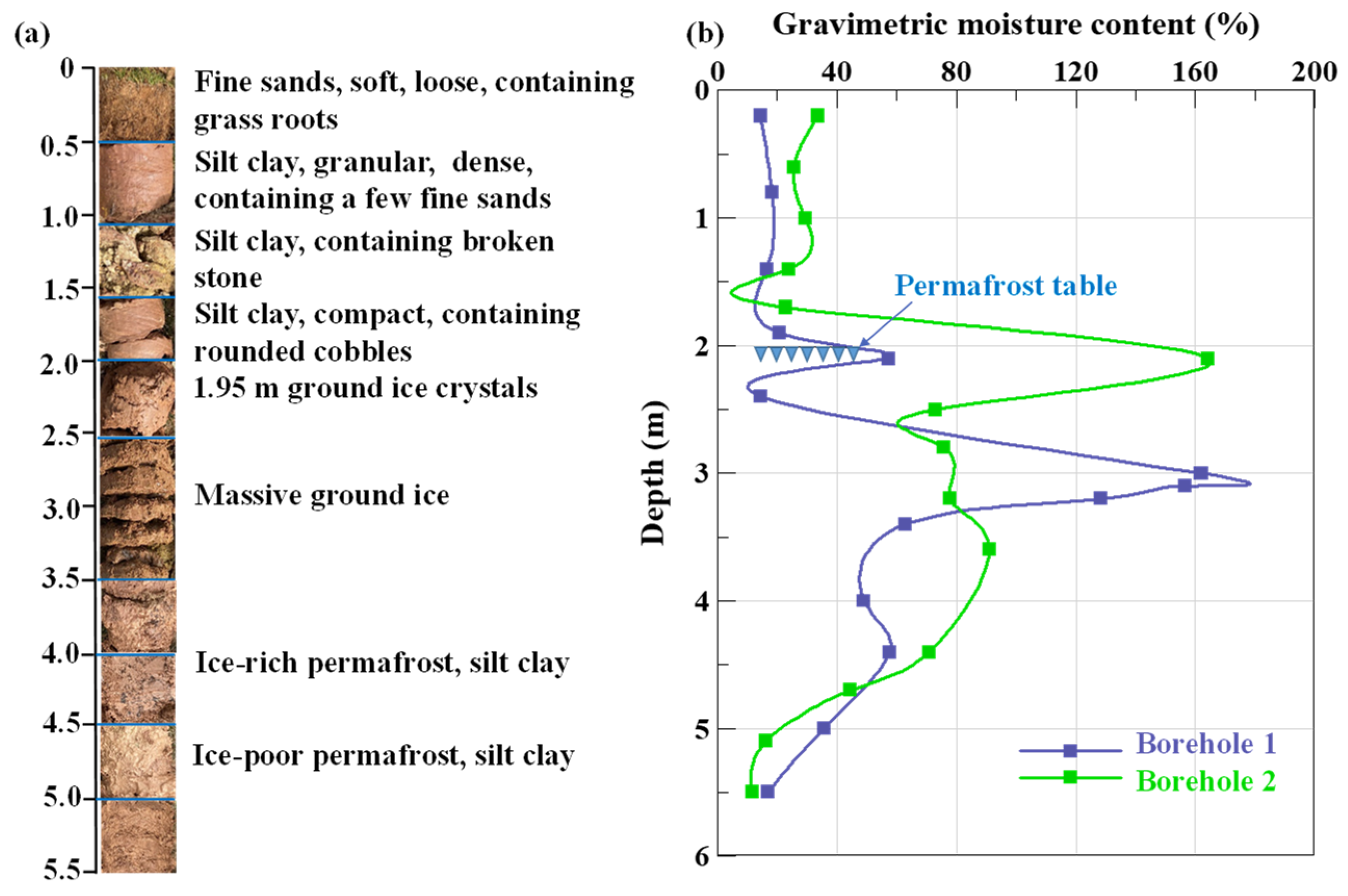
Figure 2. Longitudinal profile of the K1129W thaw slump.
Remotesensing 14 05592 g002
Figure 3. Drilling borehole information of the K1129W thaw slump. (a) Borehole logging and (b) gravimetric moisture content.
Remotesensing 14 05592 g003
Figure 5. Diagrams of numerical and in situ shear strength tests. (a) The active layer and ground ice interface; (b) a cross-section of the discrete element model; (c) in situ shear strength test setup [9]; (d) a cutting soil sample on the surface of the massive ground ice [9].
Remotesensing 14 05592 g005
Figure 6. Basic discrete element model (a), details of the headwall (b), and the three-dimensional point cloud model (c) of the K1129W thaw slump.
Remotesensing 14 05592 g006
Figure 7. Flow chart and framework of DEM-FDM in the K1129W thaw slump.
Remotesensing 14 05592 g007
Figure 8. Data acquisition and processing flowchart of terrestrial laser scanning and unmanned aerial vehicle.
Remotesensing 14 05592 g008
Figure 9. Comparison between the in situ tests and DEM simulations of horizontal stress–displacement curves. (a) Horizontal stress–displacement curves and samples after shear failure of (b) in situ test [9] and (c) discrete element test.
Remotesensing 14 05592 g009
Figure 10. Comparison of the shear stress with loading horizontal displacement with different weakening coefficients αw at vertical stresses of (a) 30.00 kPa, (b) 44.08 kPa, and (c) 50.61 kPa.
Remotesensing 14 05592 g010
Figure 11. Simulated evolution of the K1129W thaw slump. (a) Displacement evolution of related elements. (b) Velocity evolution of related elements. Note that the white solid line represents the thaw slump boundary in September 2021.
Remotesensing 14 05592 g011
Figure 12. Surface deformation (a) and headwall retrogression (b) of the K1129W thaw slump development area using terrestrial laser scanning (TLS) and unmanned aerial vehicle (UAV).
Remotesensing 14 05592 g012
Figure 13. Mass transport, headwall retrogression, and relation with volumetric ice content. (a) Box plots of volumetric change in K1129W thaw slump development area of different volumetric ice contents. (b) Linear relation between mass transport amount and volumetric ice content. (c) Box plots of headwall retrogression in K1129W thaw slump development area of different volumetric ice contents. (d) Linear relation between headwall retrogression and volumetric ice content. Note that the red short dash is the average value.
Remotesensing 14 05592 g013
Table 1. Geotechnical properties at the K1129W thaw slump site.
Depth (m)0.51.51.9Ground Ice Layer
Young modulus, E (MPa)11.684.368.66830
Poisson’s ratio0.120.190.160.14
Uniaxial tensile strength, σt (kPa)-0.65215.4
Uniaxial compressive strength, σc (kPa)-112066.5
Intergranular friction coefficient, μ0.680.550.620.2
Element density, ρ (kg/m3)185019502150917
Table 2. Physical and thermal parameters of the K1129W thaw slump model.
Properties and ParametersValues
Soil
Density of solid grains2350 kg/m3
Thermal conductivity of soil (λw)1.48 W/m/K
Specific heat of soil (cw)1041.5 J/kg/K
Permafrost
Density of ice (ρi)910 kg/m3
Density of ice-rich permafrost (50–80%)1700 kg/m3
Thermal conductivity of ice (λi)2.14 W/m/K
Thermal conductivity of ice-rich permafrost (50–80%)1.87 W/m/K
Specific heat of ice (ci)2108 J/kg/K
Specific heat of ice-rich permafrost (50–80%)1860 J/kg/K
Latent heat (Lw)3.34 × 10⁵ J/kg
Others
Shape factor for unfrozen water content q3.0
Terminal fraction of moisture unfrozen p0.165
Publisher’s Note: MDPI stays neutral with regard to jurisdictional claims in published maps and institutional affiliations.

