
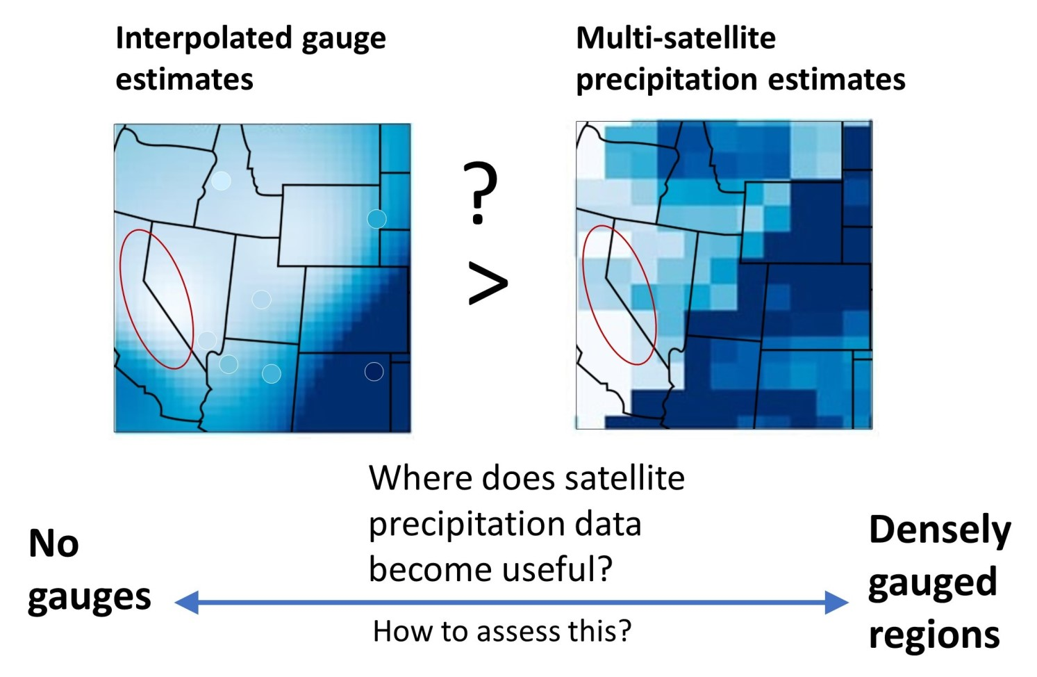
Where Can IMERG Provide a Better Precipitation Estimate than Interpolated Gauge Data?

Abstract
: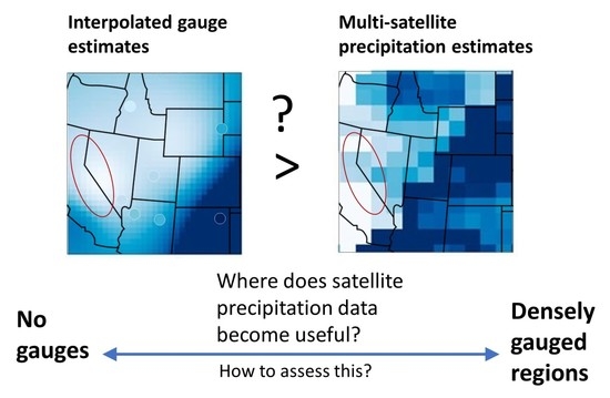
1. Introduction
2. Data
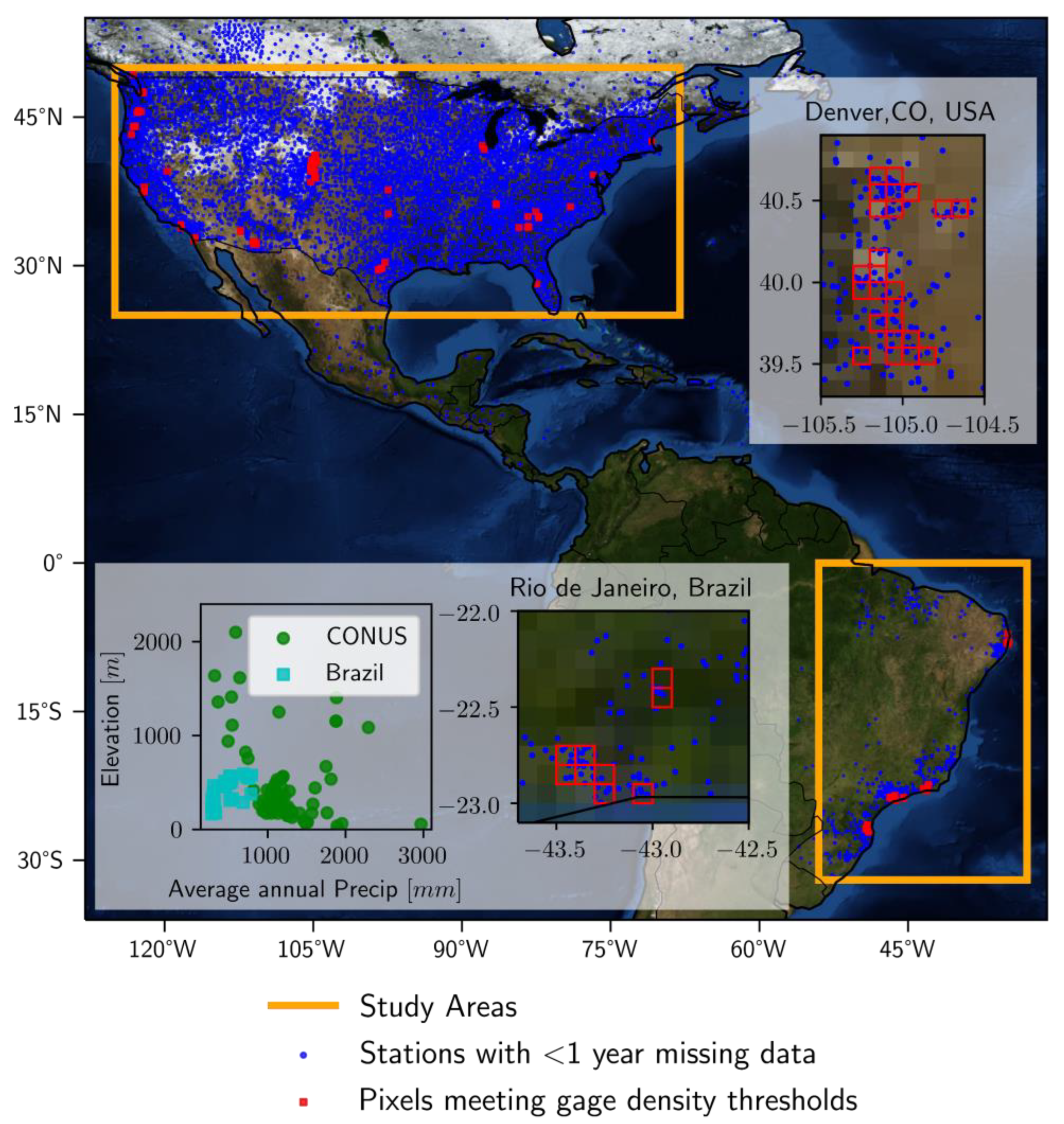
2.1. Study Area and Period
2.2. Gauge Data
2.3. Satellite Precipitation Data
3. Methods
3.1. Pixel Selection
3.2. Inverse Distance Weighting Interpolation Scheme
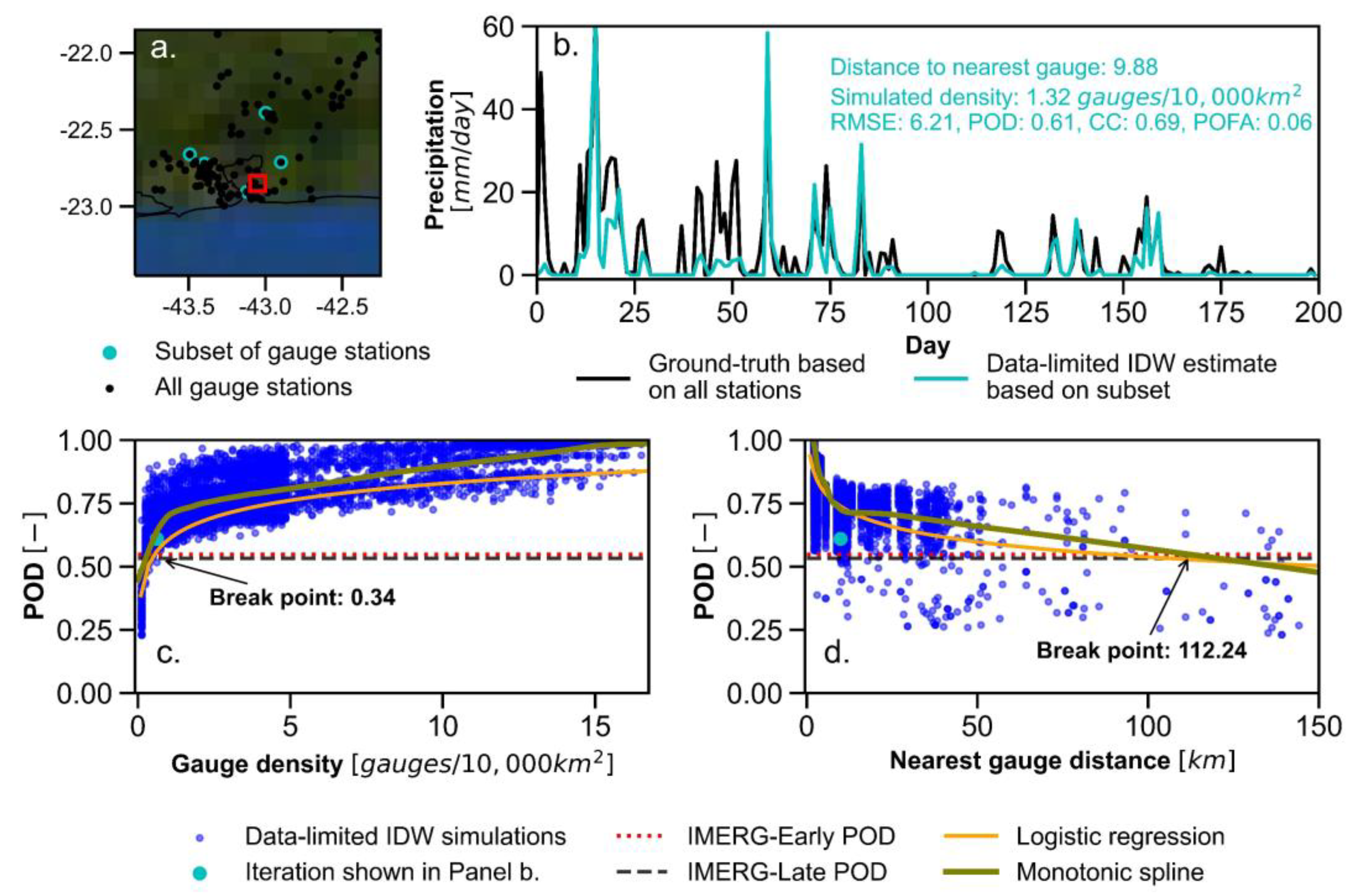
3.3. Monte Carlo “Data-Limited” Interpolation Scheme
- (a)
- n stations within 1.0° of a pixel are simulated as “available” and are used to generate a “data-limited” precipitation timeseries using IDW interpolation for that pixel (Figure 2a,b).
- (b)
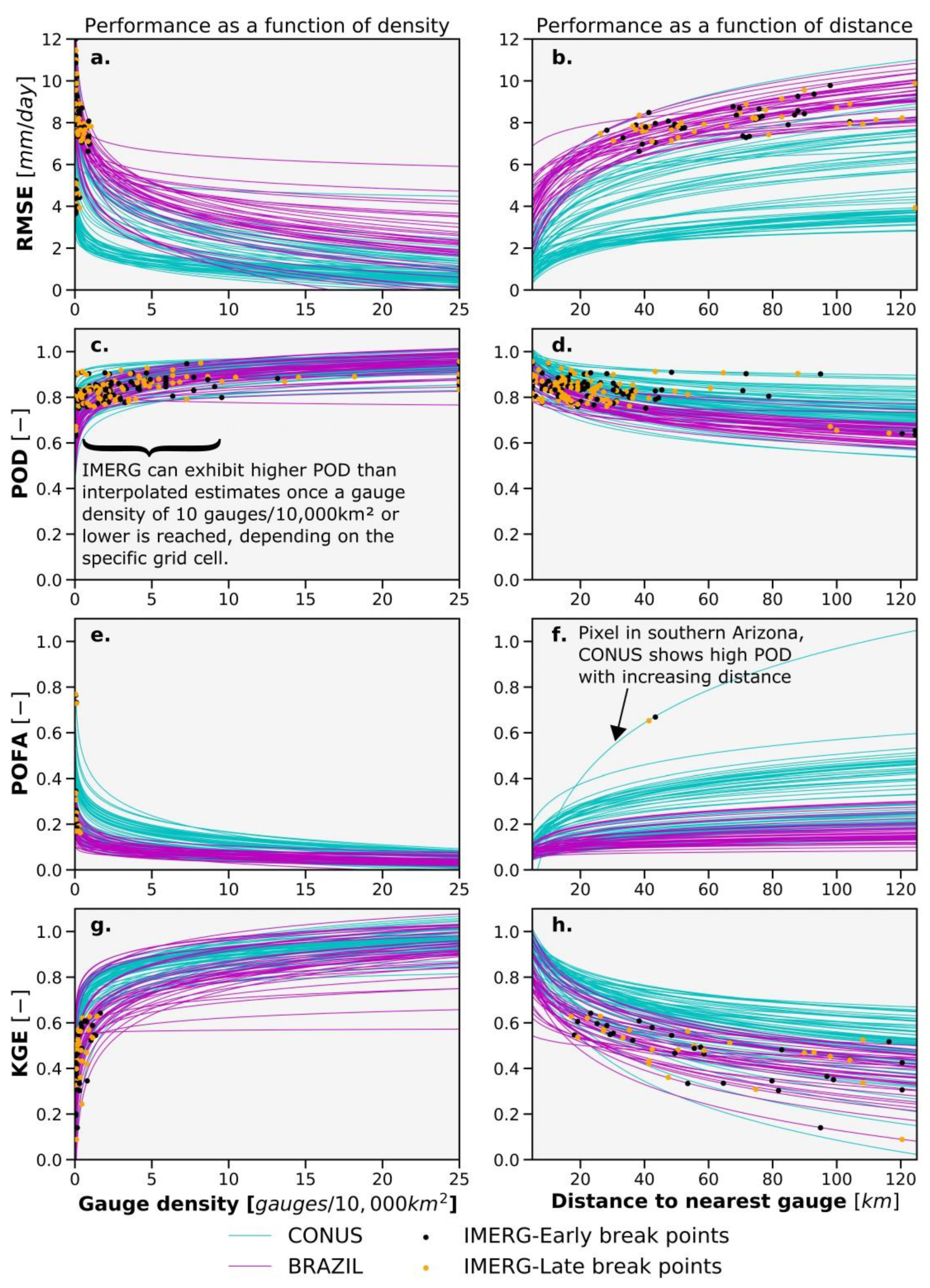
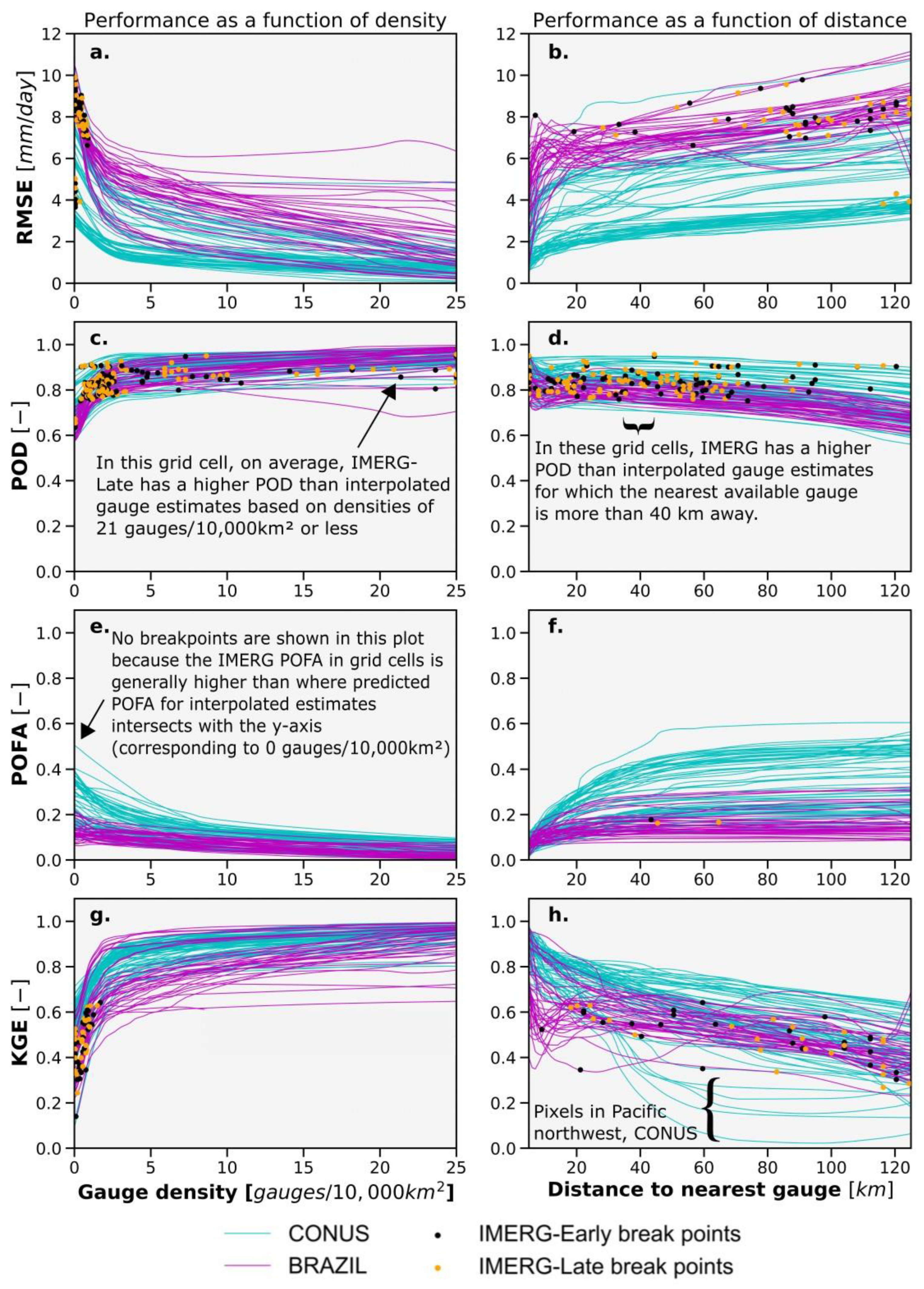
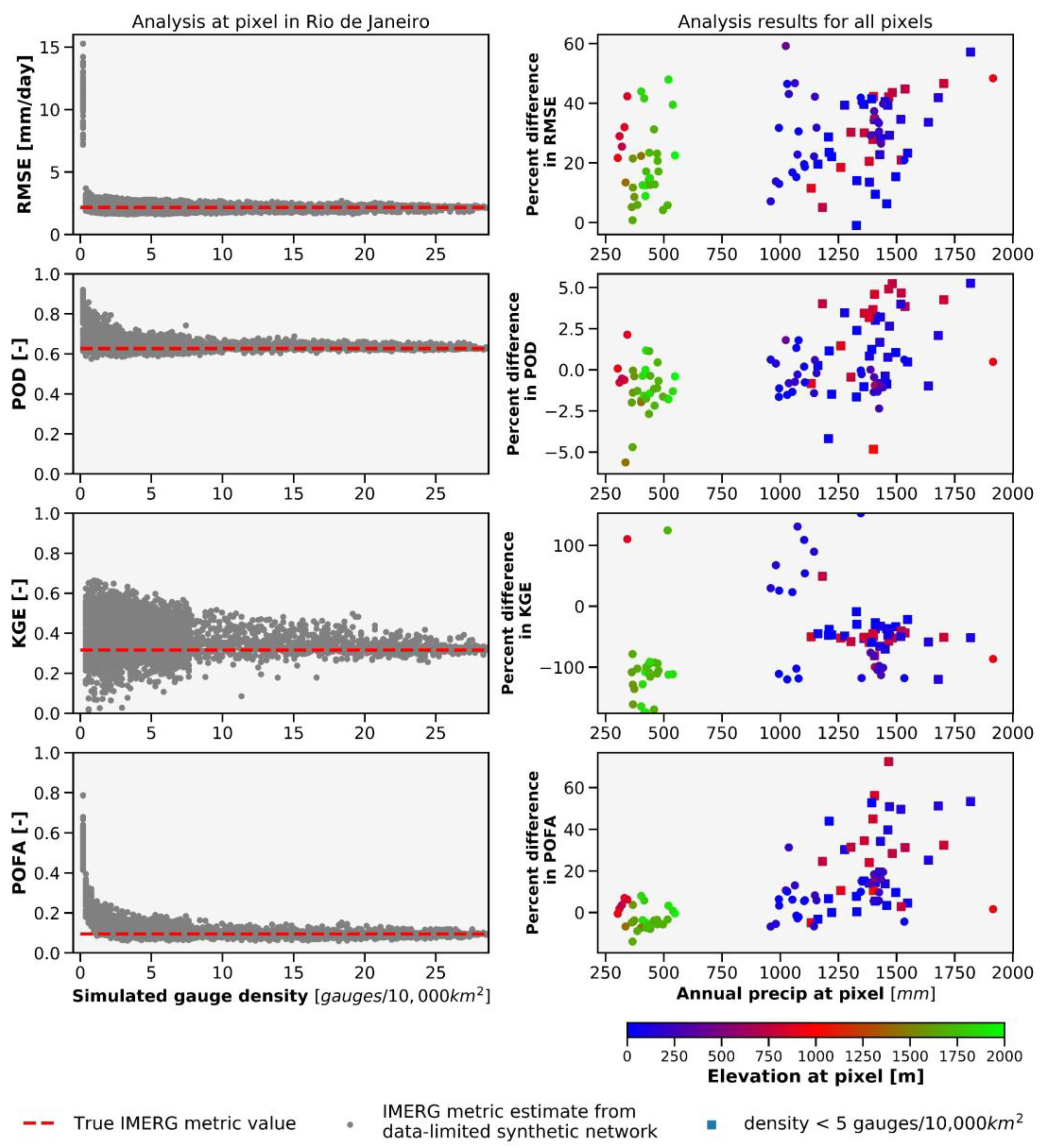
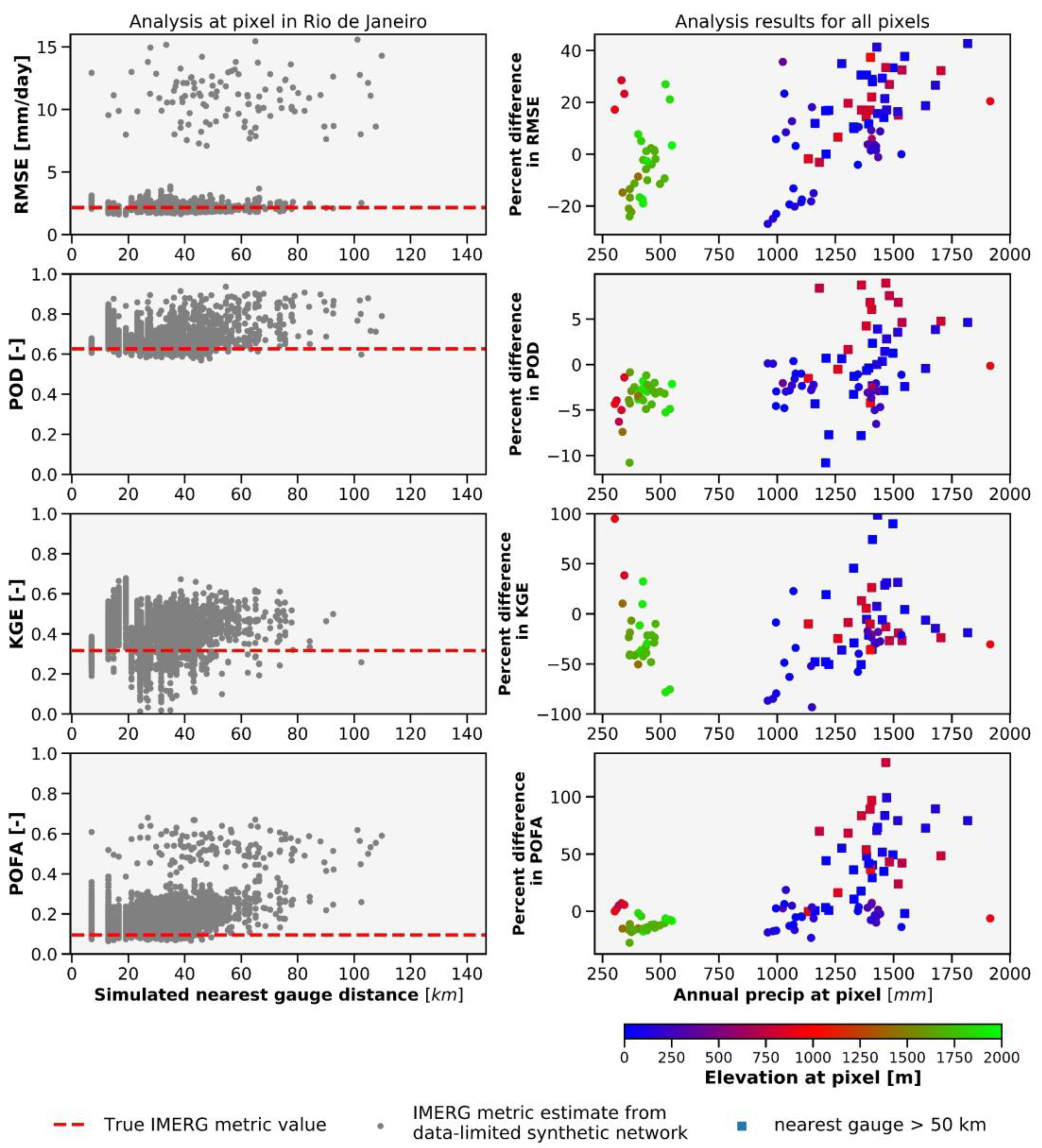
- The resulting data-limited interpolated timeseries is compared against ground-truth precipitation. The following performance metrics are calculated for the data-limited timeseries: root mean square error (RMSE), probability of detection (POD), probability of false alarm (POFA), and Kling Gupta Efficiency (KGE). These performance metrics are further described in Section 3.4.
- (c)
- This scheme is repeated for a range of values of n, from n = 1 to n = nearly all available stations, resulting in a range of POD values and other performance metric values across the range of simulated gauge densities used during data-limited interpolation (Figure 2c). For each simulated value of n, n stations are randomly selected. At least 3000 iterations are performed at each pixel with a range of values for n to simulate a large variety of gauge densities and gauge network configurations.
3.4. Performance Metrics
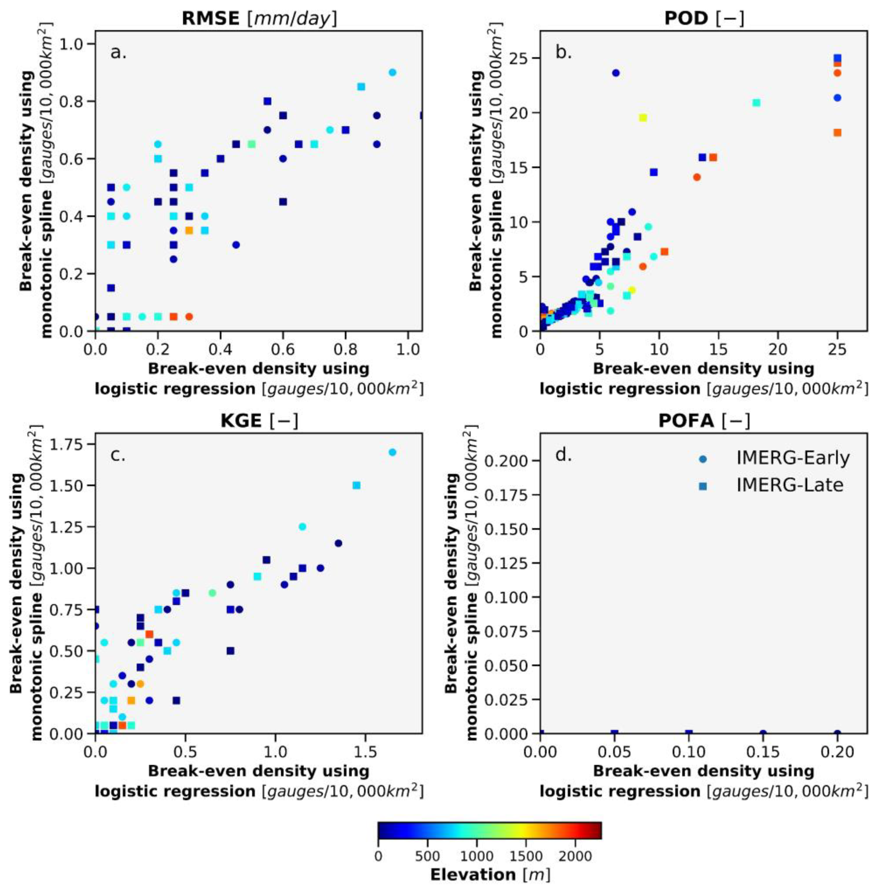
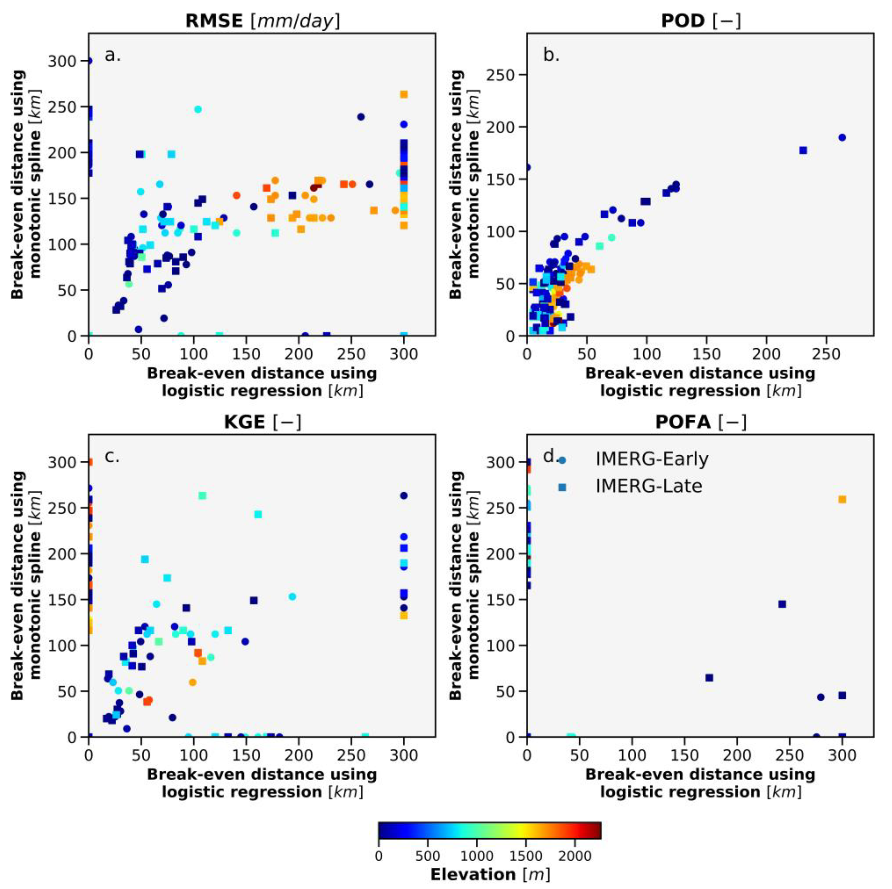
3.5. Regression Fitting
3.6. Comparison of Interpolated Gauge Performance to IMERG
3.7. Assessing the Ability of Interpolated Estimates to Evaluate IMERG
4. Results
5. Discussion
5.1. Accuracy of Interpolated Gauge Estimates as a Function of Gauge Density and Nearest Gauge Distance
5.2. Accuracy of Interpolated Gauge Estimates Relative to IMERG Early and Late
5.3. Ability of Interpolated Estimates to Evaluate IMERG
5.4. Interpolated Data Performance as a Function of Climate and Geographic Setting
6. Conclusions
Author Contributions
Funding
Data Availability Statement
Acknowledgments
Conflicts of Interest
References
- Shige, S.; Kida, S.; Ashiwake, H.; Kubota, T.; Aonashi, K. Improvement of TMI rain retrievals in mountainous areas. J. Appl. Meteorol. Climatol. 2013, 52, 242–254. [Google Scholar] [CrossRef] [Green Version]
- Tan, J.; Petersen, W.A.; Kirchengast, G.; Goodrich, D.C.; Wolff, D.B. Evaluation of global precipitation measurement rainfall estimates against three dense gauge networks. J. Hydrometeorol. 2018, 19, 517–532. [Google Scholar] [CrossRef]
- Tian, Y.; Peters-Lidard, C.D.; Choudhury, B.J.; Garcia, M. Multitemporal Analysis of TRMM-Based Satellite Precipitation Products for Land Data Assimilation Applications. J. Hydrometeorol. 2007, 8, 1165–1183. [Google Scholar] [CrossRef]
- Habib, E.H.; Meselhe, E.A.; Aduvala, A.V. Effect of Local Errors of Tipping-Bucket Rain Gauges on Rainfall-Runoff Simulations. J. Hydrol. Eng. 2008, 13, 488–496. [Google Scholar] [CrossRef]
- Kidd, C.; Becker, A.; Huffman, G.J.; Muller, C.L.; Joe, P.; Skofronick-Jackson, G.; Kirschbaum, D.B. So, how much of the Earth’s surface is covered by rain gauges? Bull. Am. Meteorol. Soc. 2017, 98, 69–78. [Google Scholar] [CrossRef] [PubMed]
- Michaelides, S.; Levizzani, V.; Anagnostou, E.; Bauer, P.; Kasparis, T.; Lane, J.E. Precipitation: Measurement, remote sensing, climatology and modeling. Atmos. Res. 2009, 94, 512–533. [Google Scholar] [CrossRef]
- Peleg, N.; Ben-Asher, M.; Morin, E. Radar subpixel-scale rainfall variability and uncertainty: Lessons learned from observations of a dense rain-gauge network. Hydrol. Earth Syst. Sci. 2013, 17, 2195–2208. [Google Scholar] [CrossRef] [Green Version]
- Sun, Q.; Miao, C.; Duan, Q.; Ashouri, H.; Sorooshian, S.; Hsu, K.L. A Review of Global Precipitation Data Sets: Data Sources, Estimation, and Intercomparisons. Rev. Geophys. 2018, 56, 79–107. [Google Scholar] [CrossRef] [Green Version]
- Villarini, G.; Mandapaka, P.V.; Krajewski, W.F.; Moore, R.J. Rainfall and sampling uncertainties: A rain gauge perspective. J. Geophys. Res. Atmos. 2008, 113, 11102. [Google Scholar] [CrossRef]
- Freitas, E.d.S.; Coelho, V.H.R.; Xuan, Y.; Melo, D.d.C.D.; Gadelha, A.N.; Santos, E.A.; Galvão, C.d.O.; Ramos Filho, G.M.; Barbosa, L.R.; Huffman, G.J.; et al. The performance of the IMERG satellite-based product in identifying sub-daily rainfall events and their properties. J. Hydrol. 2020, 589, 125128. [Google Scholar] [CrossRef]
- Xavier, A.C.; King, C.W.; Scanlon, B.R. Daily gridded meteorological variables in Brazil (1980–2013). Int. J. Climatol. 2016, 36, 2644–2659. [Google Scholar] [CrossRef] [Green Version]
- Xu, H.; Xu, C.Y.; Chen, H.; Zhang, Z.; Li, L. Assessing the influence of rain gauge density and distribution on hydrological model performance in a humid region of China. J. Hydrol. 2013, 505, 1–12. [Google Scholar] [CrossRef]
- Mishra, A.K. Effect of Rain Gauge Density over the Accuracy of Rainfall: A Case Study Over Bangalore; SpringerPlus: Delhi, India, 2013; Volume 2, pp. 1–7. [Google Scholar] [CrossRef] [Green Version]
- Otieno, H.; Yang, J.; Liu, W.; Han, D. Influence of Rain Gauge Density on Interpolation Method Selection. J. Hydrol. Eng. 2014, 19, 04014024. [Google Scholar] [CrossRef]
- Prakash, S.; Mitra, A.K.; Pai, D.S.; AghaKouchak, A. From TRMM to GPM: How well can heavy rainfall be detected from space? Adv. Water Resour. 2016, 88, 1–7. [Google Scholar] [CrossRef]
- Nikolopoulos, E.I.; Borga, M.; Creutin, J.D.; Marra, F. Estimation of debris flow triggering rainfall: Influence of rain gauge density and interpolation methods. Geomorphology 2015, 243, 40–50. [Google Scholar] [CrossRef]
- Anjum, M.N.; Ding, Y.; Shangguan, D.; Ahmad, I.; Wajid Ijaz, M.; Farid, H.U.; Yagoub, Y.E.; Zaman, M.; Adnan, M. Performance evaluation of latest integrated multi-satellite retrievals for Global Precipitation Measurement (IMERG) over the northern highlands of Pakistan. Atmos. Res. 2018, 205, 134–146. [Google Scholar] [CrossRef]
- Gadelha, A.N.; Coelho, V.H.R.; Xavier, A.C.; Barbosa, L.R.; Melo, D.C.D.; Xuan, Y.; Huffman, G.J.; Petersen, W.A.; Almeida, C. das N. Grid box-level evaluation of IMERG over Brazil at various space and time scales. Atmos. Res. 2019, 218, 231–244. [Google Scholar] [CrossRef] [Green Version]
- Tian, F.; Hou, S.; Yang, L.; Hu, H.; Hou, A. How does the evaluation of the gpm imerg rainfall product depend on gauge density and rainfall intensity? J. Hydrometeorol. 2018, 19, 339–349. [Google Scholar] [CrossRef]
- Villarini, G. Evaluation of the Research-Version TMPA Rainfall Estimate at Its Finest Spatial and Temporal Scales over the Rome Metropolitan Area. J. Appl. Meteorol. Climatol. 2010, 49, 2591–2602. [Google Scholar] [CrossRef]
- Mandapaka, P.V.; Lo, E.Y.M. Evaluation of GPM IMERG Rainfall Estimates in Singapore and Assessing Spatial Sampling Errors in Ground Reference. J. Hydrometeorol. 2020, 21, 2963–2977. [Google Scholar] [CrossRef]
- Girons Lopez, M.; Wennerström, H.; Nordén, L.Å.; Seibert, J. Location and density of rain gauges for the estimation of spatial varying precipitation. Geogr. Ann. Ser. A Phys. Geogr. 2015, 97, 167–179. [Google Scholar] [CrossRef] [Green Version]
- Villarini, G.; Krajewski, W.F. Evaluation of the research version TMPA three-hourly 0.25° × 0.25° rainfall estimates over Oklahoma. Geophys. Res. Lett. 2007, 34, 1–5. [Google Scholar] [CrossRef]
- Almeida, C.; Coelho, V.H.R.; Meira, M.A.; Carvalho, F. Boletim Anual de Precipitação no Brasil (ano 2021); Federal University of Paraíba: Paraíba, Brazil, 2022. [Google Scholar]
- Tang, G.; Clark, M.P.; Newman, A.J.; Wood, A.W.; Papalexiou, S.M.; Vionnet, V.; Whitfield, P.H. SCDNA: A serially complete precipitation and temperature dataset for North America from 1979 to 2018. In Earth System Science Data; Copernicus GmbH: Göttingen, Germany, 2020; Volume 12, pp. 2381–2409. [Google Scholar] [CrossRef]
- Huffman, G.; Bolvin, D.T.; Braithwaite, D.; Hsu, K.; Joyce, R.; Kidd, C.; Nelkin, E.J.; Sorooshian, S.; Tan, J.; Xie, P. NASA Global Precipitation Measurement (GPM) Integrated Multi-satellitE Retrievals for GPM (IMERG) Prepared for: Global Precipitation Measurement (GPM) National Aeronautics and Space Administration (NASA). In Algorithm Theoretical Basis Document (ATBD); NASA: Washington, DC, USA, 2019. [Google Scholar]
- Tan, J.; Huffman, G.J.; Bolvin, D.T.; Nelkin, E.J. IMERG V06: Changes to the morphing algorithm. J. Atmos. Ocean. Technol. 2019, 36, 2471–2482. [Google Scholar] [CrossRef]
- Stanley, T.A.; Kirschbaum, D.B.; Benz, G.; Emberson, R.A.; Amatya, P.M.; Medwedeff, W.; Clark, M.K. Data-Driven Landslide Nowcasting at the Global Scale. Front. Earth Sci. 2021, 9, 1–15. [Google Scholar] [CrossRef]
- Yin, J.; Guo, S.; Gu, L.; Zeng, Z.; Liu, D.; Chen, J.; Shen, Y.; Xu, C.Y. Blending multi-satellite, atmospheric reanalysis and gauge precipitation products to facilitate hydrological modelling. J. Hydrol. 2021, 593, 125878. [Google Scholar] [CrossRef]
- Zhou, Y.; Nelson, K.; Mohr, K.I.; Huffman, G.J.; Levy, R.; Grecu, M. A Spatial-Temporal Extreme Precipitation Database from GPM IMERG. J. Geophys. Res. Atmos. 2019, 124, 10344–10363. [Google Scholar] [CrossRef]
- Ly, S.; Charles, C.; Degré, A. Geostatistical interpolation of daily rainfall at catchment scale: The use of several variogram models in the Ourthe and Ambleve catchments, Belgium. Hydrol. Earth Syst. Sci. 2011, 15, 2259–2274. [Google Scholar] [CrossRef] [Green Version]
- Tan, J.; Petersen, W.; Tokay, A. A Novel Approach to Identify Sources of Errors in IMERG for GPM Ground Validation. J. Hydrometeorol. 2016, 17, 2477–2491. [Google Scholar] [CrossRef]
- Linfei, Y.; Leng, G.; Python, A.; Peng, J. A Comprehensive Evaluation of Latest GPM IMERG V06 Early, Late and Final Precipitation Products across China. Remote Sens. 2021, 13, 1208. [Google Scholar] [CrossRef]
- Utreras, F.I. Smoothing noisy data under monotonicity constraints existence, characterization and convergence rates. Numer. Math. 1985, 47, 611–625. [Google Scholar] [CrossRef]
- Zhang, J.T. A simple and efficient monotone smoother using smoothing splines. J. Nonparametric Stat. 2004, 16, 779–796. [Google Scholar] [CrossRef]
- Virtanen, P.; Gommers, R.; Oliphant, T.E.; Haberland, M.; Reddy, T.; Cournapeau, D.; Burovski, E.; Peterson, P.; Weckesser, W.; Bright, J.; et al. SciPy 1.0: Fundamental algorithms for scientific computing in Python. Nat. Methods 2020, 17, 261–272. [Google Scholar] [CrossRef] [PubMed] [Green Version]
- Wang, S.; Liu, J.; Wang, J.; Qiao, X.; Zhang, J. Evaluation of GPM IMERG V05B and TRMM 3B42V7 Precipitation products over high mountainous tributaries in Lhasa with dense rain gauges. Remote Sens. 2019, 11, 2080. [Google Scholar] [CrossRef]


| CONUS Average | Brazil Average | |||
|---|---|---|---|---|
| Break-Even Density [Gauges/10,000 km2] | Break-Even Distance [km] | Break-Even Density [Gauges/10,000 km2] | Break-Even Distance [km] | |
| RMSE [mm/day] | 0.1 ± 0.1 (0.1 ± 0.1) | 178 ± 38 (175 ± 35) | 0.4 ± 0.3 (0.4 ± 0.2) | 100 ± 45 (105 ± 40) |
| KGE [-] | 0.3 ± 0.3 (0.2 ± 0.2) | 172 ± 59 (179 ± 61) | 0.6 ± 0.4 (0.5 ± 0.4) | 94 ± 53 (113 ± 58) |
| POD [-] | 4.7 ± 6.1 (5.9 ± 7.0) | 42 ± 31 (38 ± 27) | 2.4 ± 3.8 (1.6 ± 0.8) | 47 ± 48 (46 ± 45) |
| POFA [-] | -- | 246 ± 42 (246 ± 41) | -- | 196 ± 58 (182 ± 65) |
Publisher’s Note: MDPI stays neutral with regard to jurisdictional claims in published maps and institutional affiliations. |
© 2022 by the authors. Licensee MDPI, Basel, Switzerland. This article is an open access article distributed under the terms and conditions of the Creative Commons Attribution (CC BY) license (https://creativecommons.org/licenses/by/4.0/).
Share and Cite
Hartke, S.H.; Wright, D.B. Where Can IMERG Provide a Better Precipitation Estimate than Interpolated Gauge Data? Remote Sens. 2022, 14, 5563. https://doi.org/10.3390/rs14215563
Hartke SH, Wright DB. Where Can IMERG Provide a Better Precipitation Estimate than Interpolated Gauge Data? Remote Sensing. 2022; 14(21):5563. https://doi.org/10.3390/rs14215563
Chicago/Turabian StyleHartke, Samantha H., and Daniel B. Wright. 2022. "Where Can IMERG Provide a Better Precipitation Estimate than Interpolated Gauge Data?" Remote Sensing 14, no. 21: 5563. https://doi.org/10.3390/rs14215563