
Improved LSTM Model for Boreal Forest Height Mapping Using Sentinel-1 Time Series


Abstract
:1. Introduction
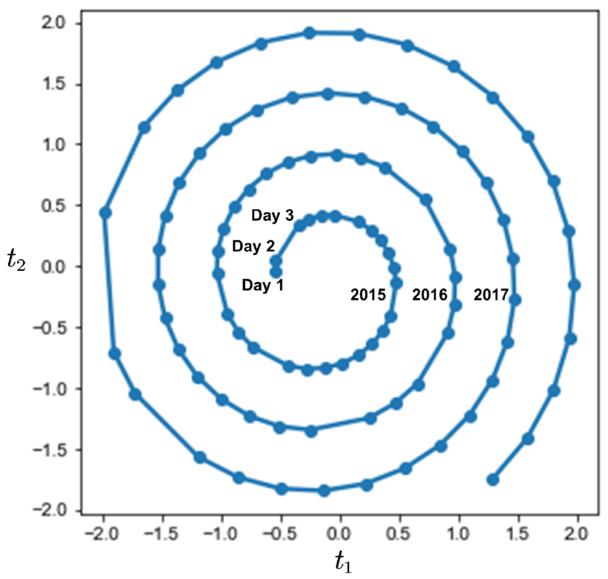
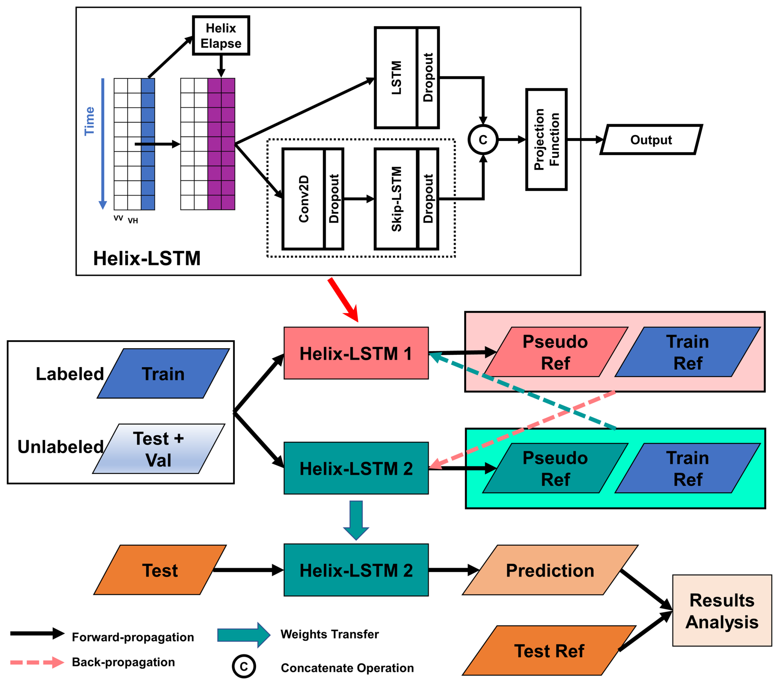
- We introduce timestamps as an additional feature to better capture the relationship between SAR backscatter and forest variables. To accommodate possible irregular intervals between image datatakes, we propose a novel Helix-Elapse (HE) projection to explicitly model the circular seasonality pattern of the long image time series.
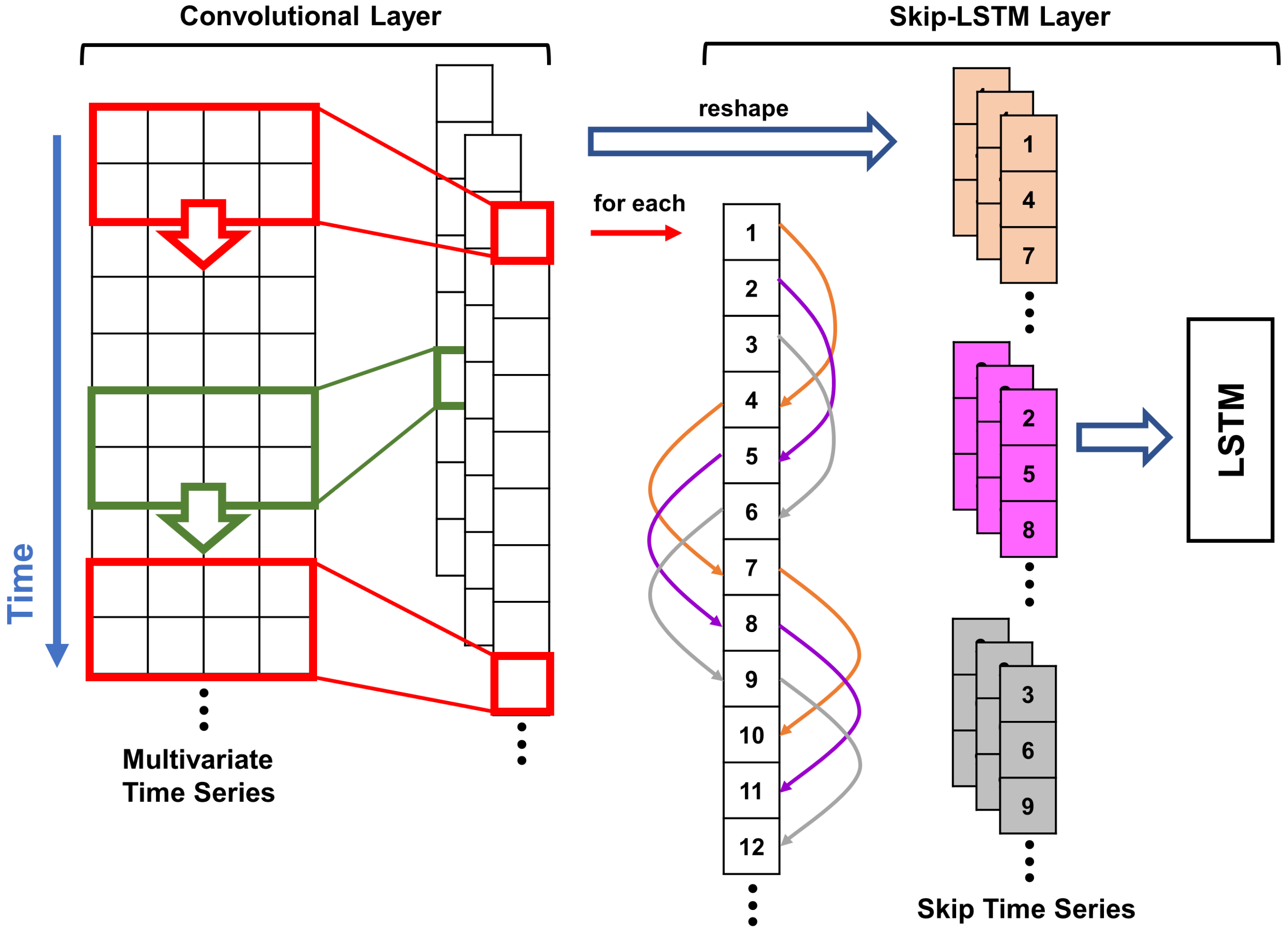
- We introduce Skip-LSTM, a hybrid LSTM block featuring with skip-link structure to better capture long-term dependencies in time series data.
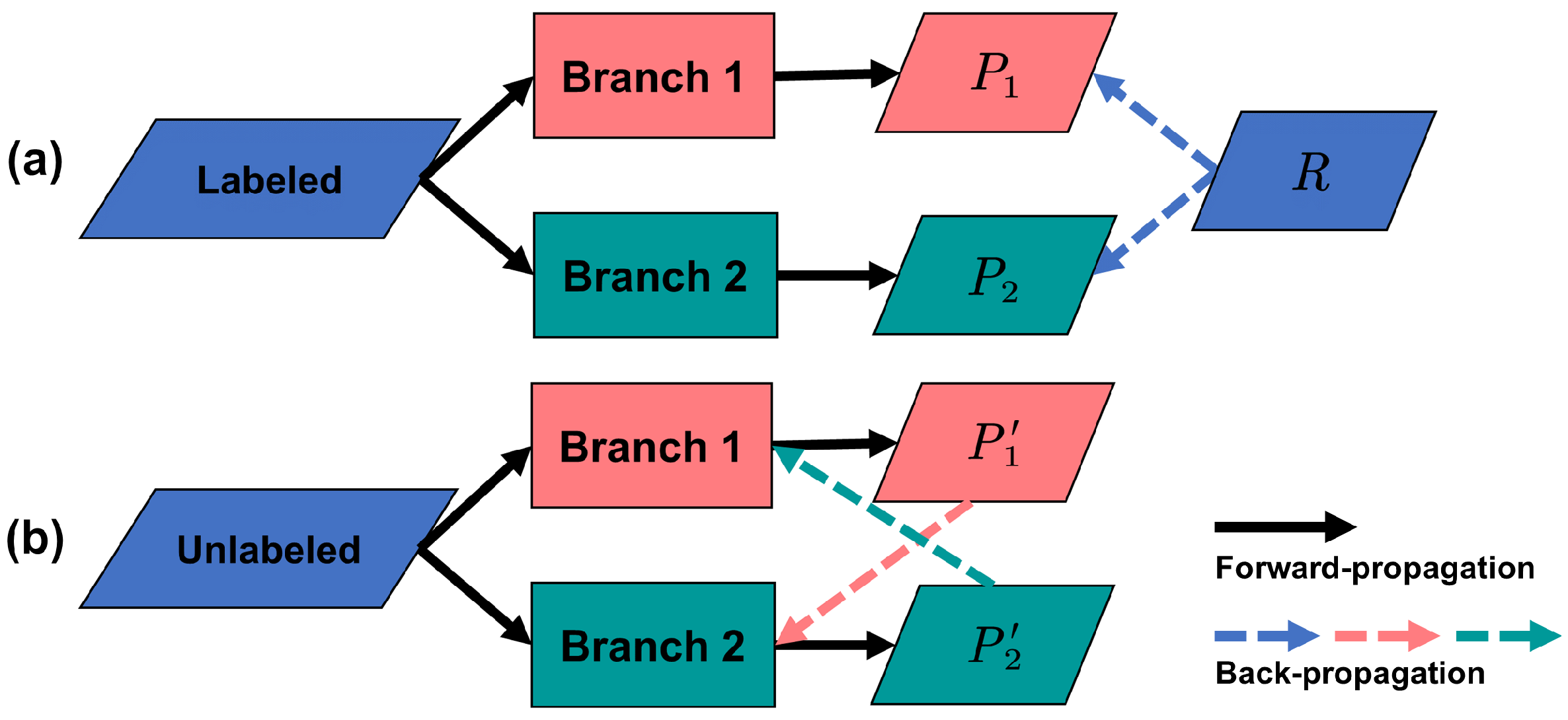
- We employ a novel semi-supervised strategy called Cross-Pseudo Regression (CPR) to improve the model prediction performance with limited reference data.
- We benchmark the developed improved LSTM model with other state-of-the-art versions of LSTM, as well as more conventional machine learning and statistical models, for the purpose of most precise forest height predictions using Sentinel-1 time series data. To the best of our knowledge, this is the first use of LSTM modeling of any kind for the purpose of forest inventory mapping.
2. Materials
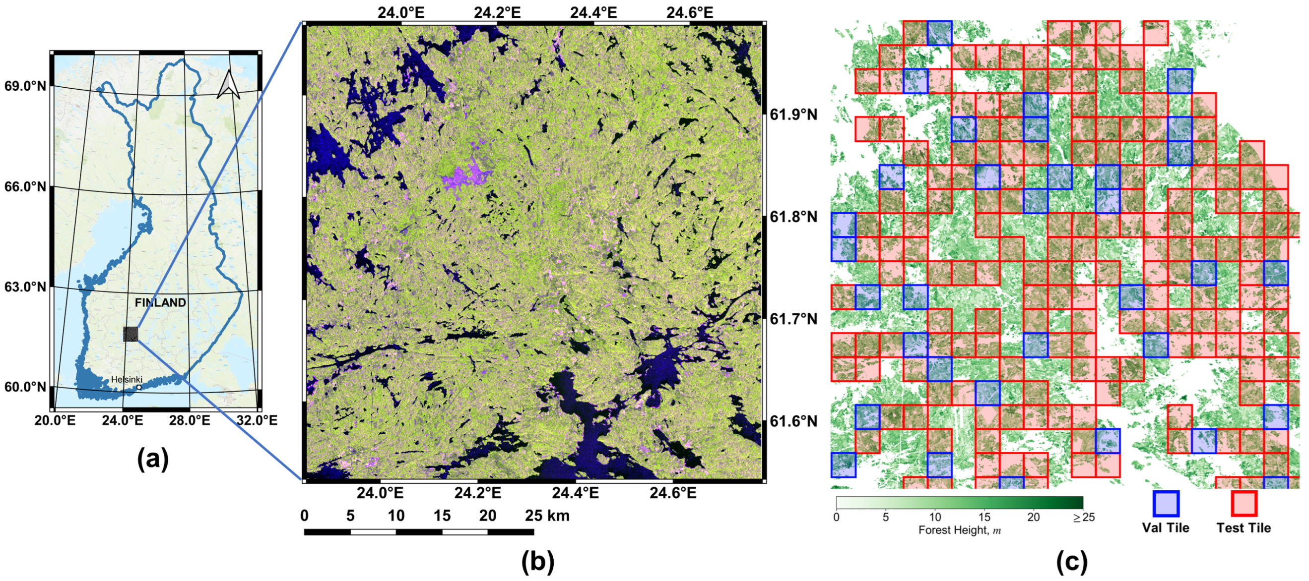
2.1. Study Site
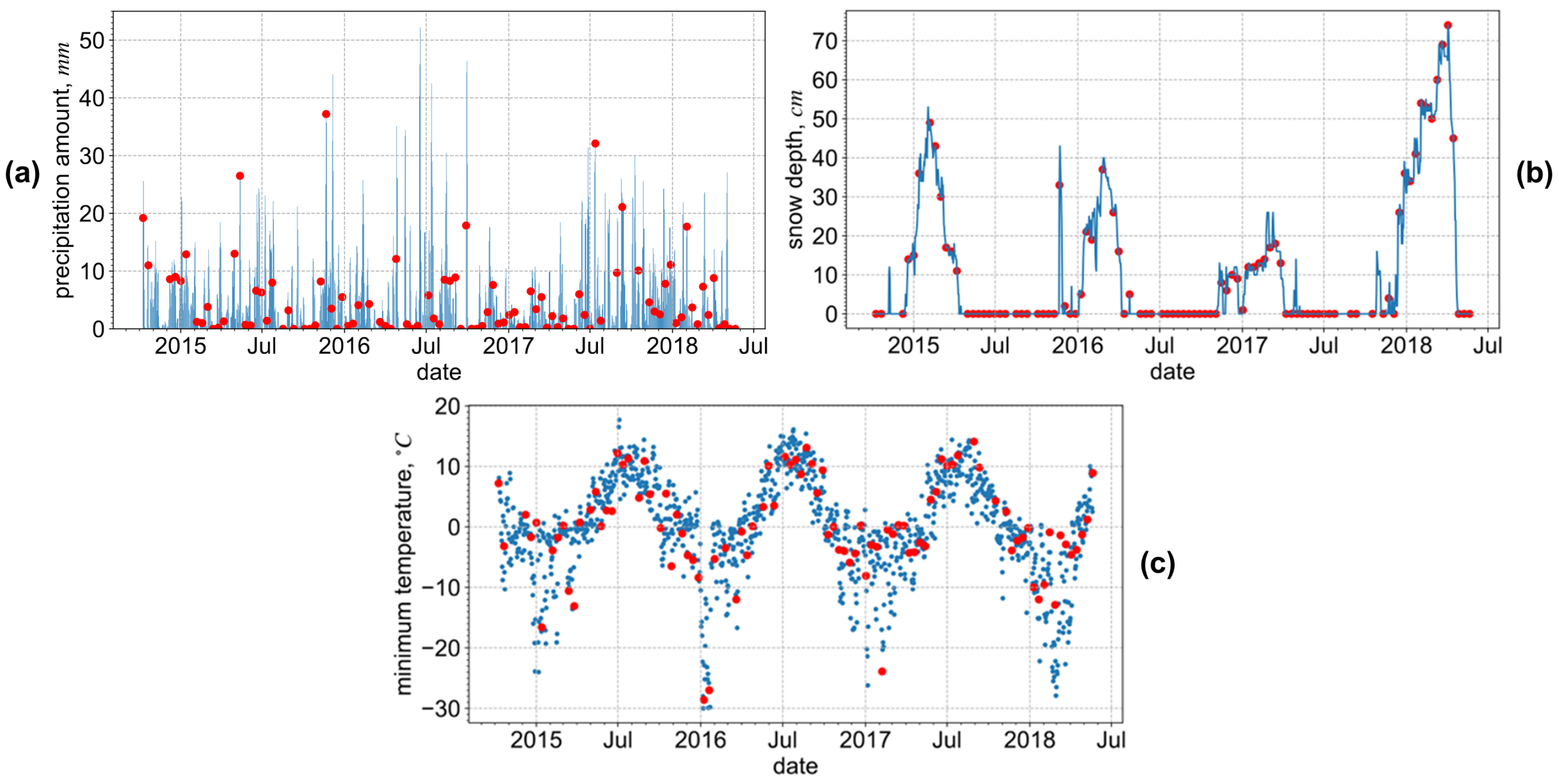
2.2. SAR and Reference Data
3. Methods
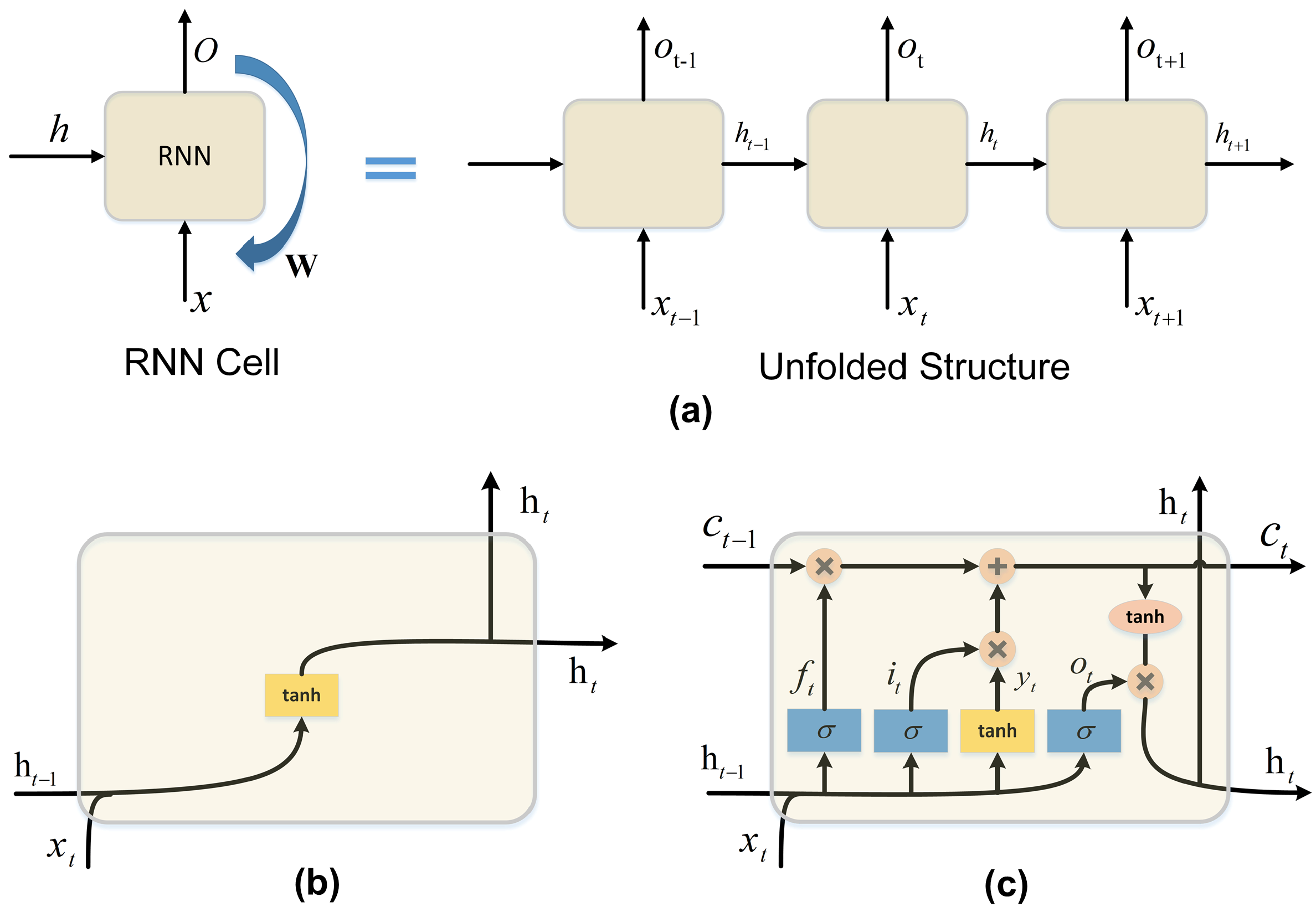
3.1. Long Short-Term Memory Networks
3.2. Helix-Elapse Projection
3.3. Skip-LSTM
3.4. Cross-Pseudo Regression
3.5. Overall Structure of CrsHelix-LSTM Model
| Algorithm 1: Training Procedure of CrsHelix-LSTM |
Input: The semi-labeled training time series ; The reference of labeled subset ; Input: Iteration number K;
|
3.6. Baseline Models
- MLR, RF, LightGBMMultiple Linear Regression (MLR) and Random Forest (RF) are mature regression methods, which have been widely used in forest remote sensing tasks. Light Gradient Boosting Machine (LightGBM) [49] is a modern Gradient Boosting Decision Tree (GBDT) model. Since being proposed by Microsoft in 2017, its precision and efficiency in regression have been proven in different application areas [50,51].
- LSTM, Attn-BiLSTMSince the proposed model is an improved version of LSTM, basic LSTM and its variant, Bidirectional LSTM with attention mechanism (Attn-BiLSTM) [33,52], are also included as baseline models for comparison. Bidirectional LSTM (BiLSTM) consists of two LSTMs with the same structure but opposite directions. Temporal dependencies are obtained from both directions. Furthermore, with the self-attention mechanism, attention weights establish the correlations between timestamps, which reportedly can better address the gradient vanishing problem and obtain long-term correlations [53]. Attn-BiLSTM combines both features and has been introduced into SAR remote sensing tasks [33].
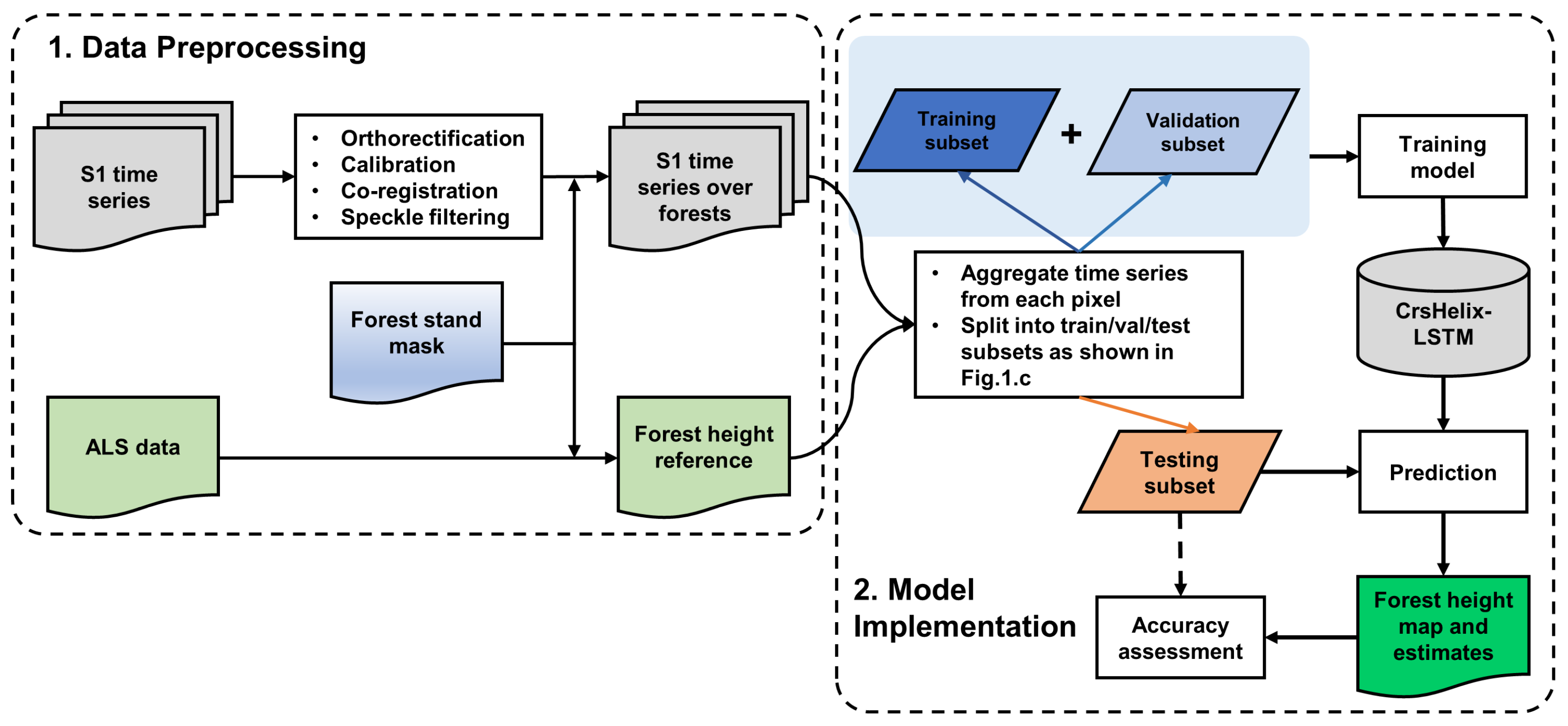
3.7. Method Implementation
3.8. Model Performance Accuracy Assessment
4. Experimental Results
4.1. Experimental Settings
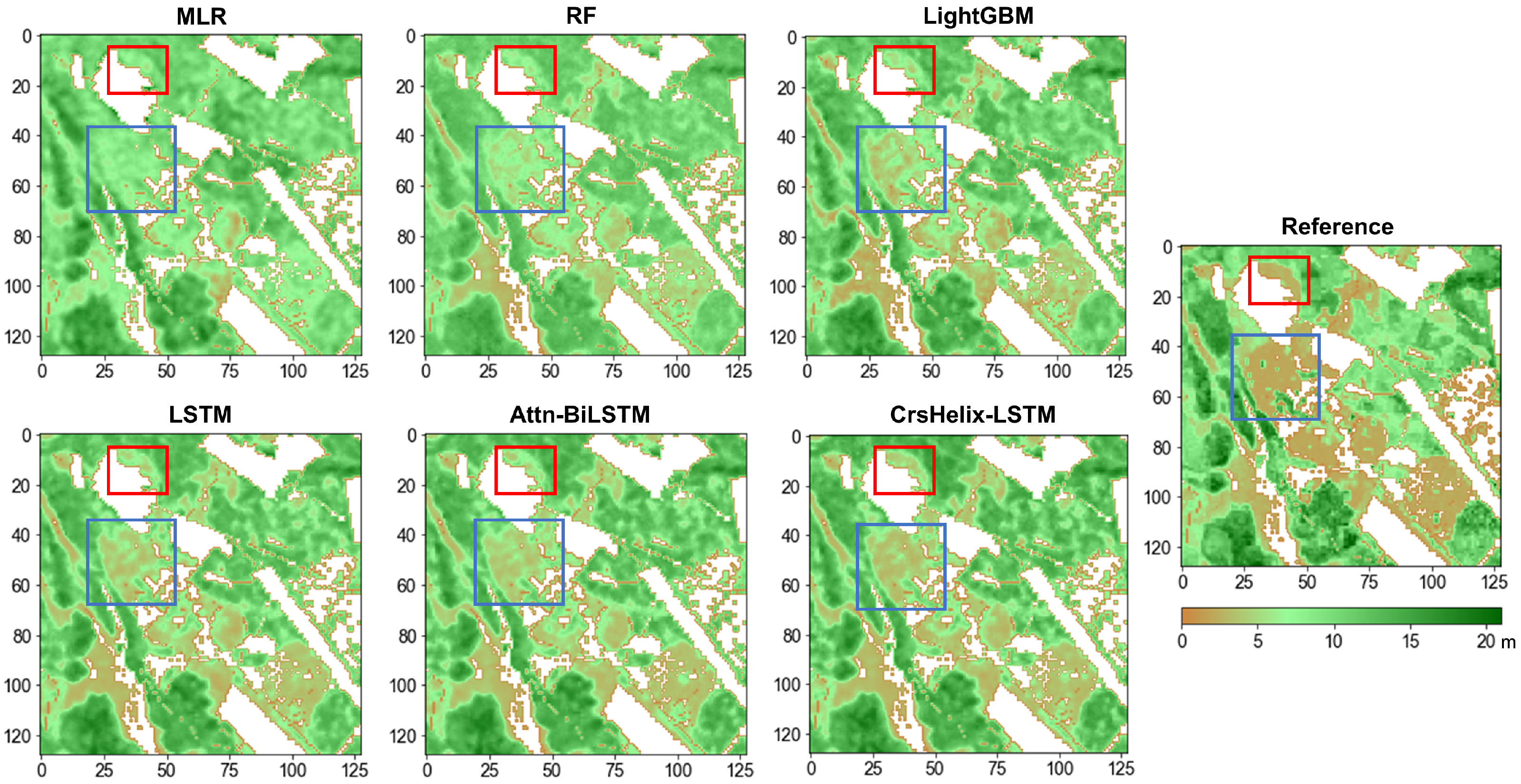
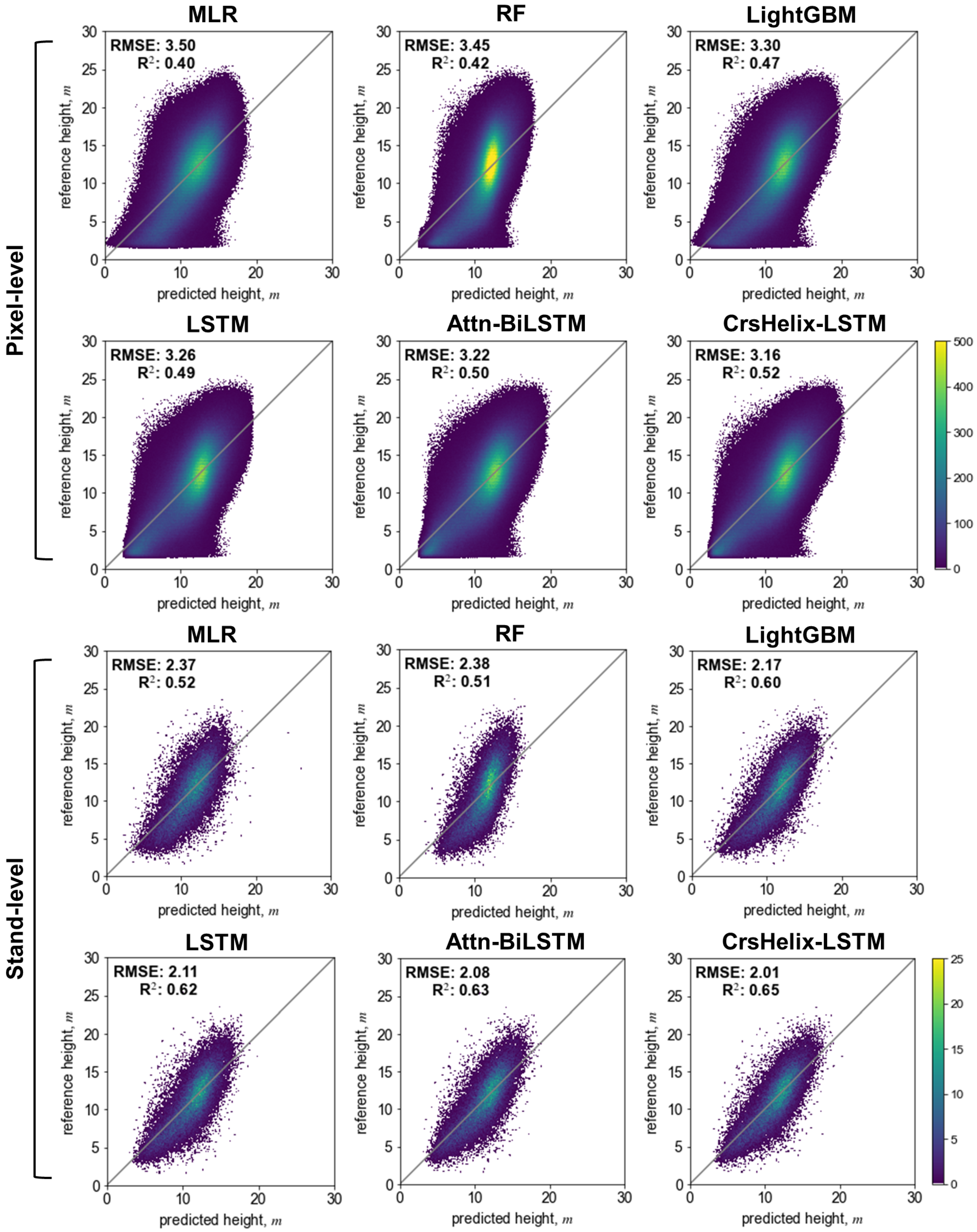
4.2. General Performance Evaluation
4.2.1. Ablation Study
4.2.2. Method Performance Comparison with Baseline Approaches
5. Discussion
5.1. Computational Complexity Analysis
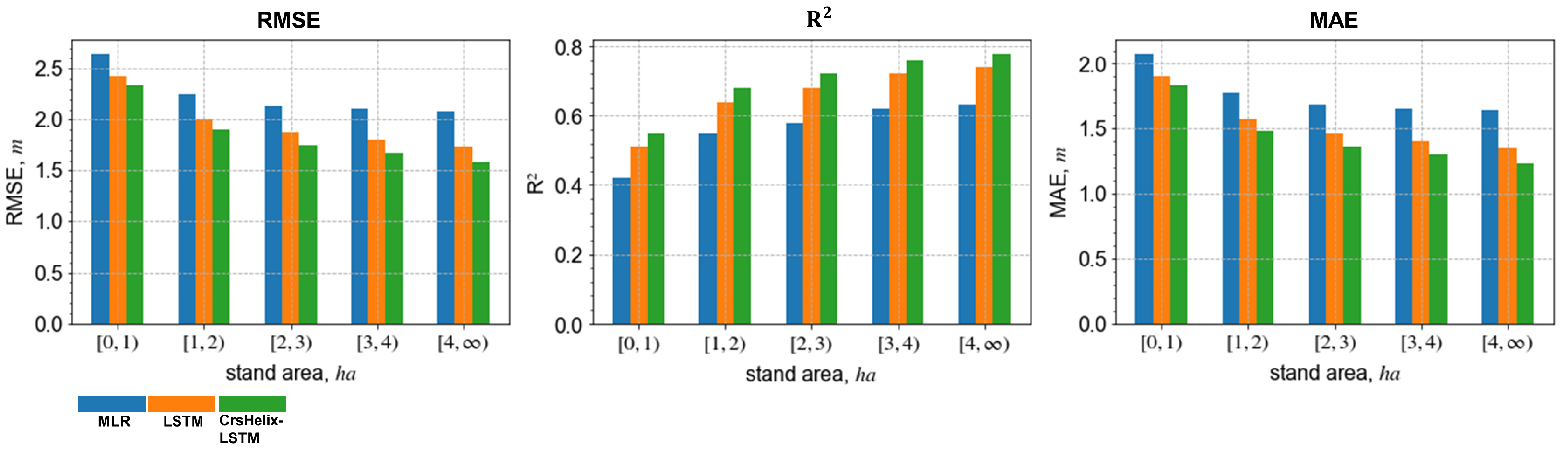
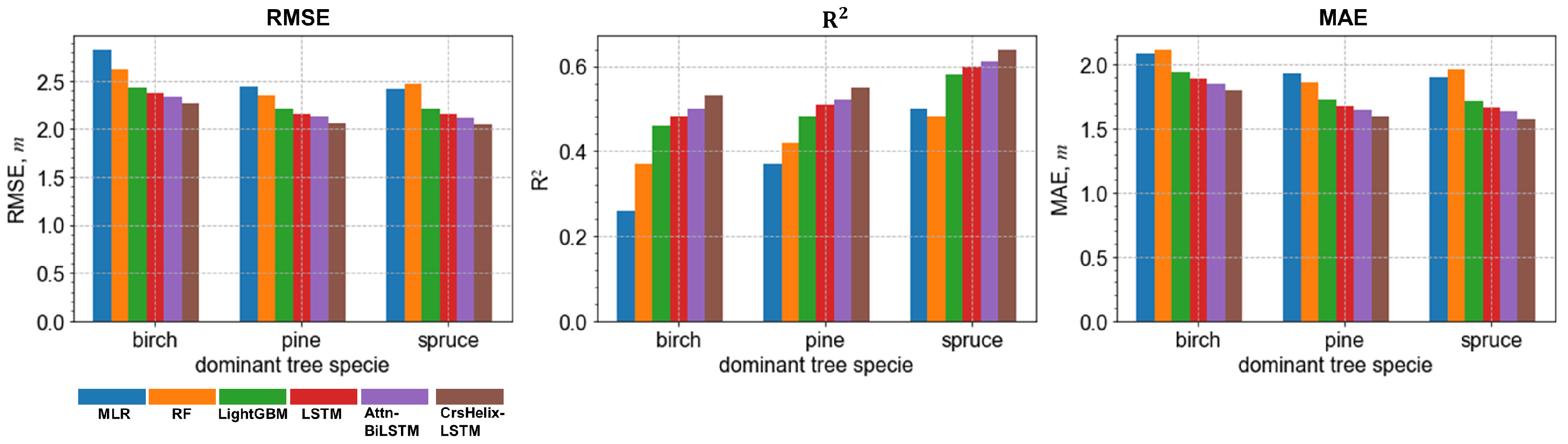
5.2. Stand-Level Performance against Different Stand Sizes and Dominant Tree Species
5.3. Comparison with Other Studies and Outlook
6. Conclusions
Author Contributions
Funding
Data Availability Statement
Conflicts of Interest
Abbreviations
| ALS | airborne laser scanning |
| Attn-BiLSTM | Bidirectional LSTM with attention mechanism |
| BiLSTM | Bidirectional LSTM |
| CNN | convolutional neural network |
| CPR | Cross-Pseudo Regression |
| CrsHelix-LSTM | Cross Helix LSTM |
| EO | earth observation |
| ESA | European Space Agency |
| FLOPs | floating point operations |
| GBDT | Gradient Boosting Decision Tree |
| GRD | ground range detected |
| HE | Helix-Elapse |
| IOA | index of agreement |
| LE | Linear-Elapse |
| LightGBM | Light Gradient Boosting Machine |
| LSTM | Long Short-Term Memory |
| MAE | mean absolute error |
| ML | machine learning |
| MLR | Multiple Linear Regression |
| MSE | mean squared error |
| PCA | principal component analysis |
| ReLU | rectified linear unit |
| RF | Random Forest |
| RMSE | root mean squared error |
| RNN | recurrent neural network |
| rRMSE | relative root mean squared error |
| SAR | synthetic aperture radar |
References
- Herold, M.; Carter, S.; Avitabile, V.; Espejo, A.B.; Jonckheere, I.; Lucas, R.; McRoberts, R.E.; Næsset, E.; Nightingale, J.; Petersen, R.; et al. The role and need for space-based forest biomass-related measurements in environmental management and policy. Surv. Geophys. 2019, 40, 757–778. [Google Scholar] [CrossRef] [Green Version]
- McRoberts, R.E.; Tomppo, E.O. Remote sensing support for national forest inventories. Remote Sens. Environ. 2007, 110, 412–419. [Google Scholar] [CrossRef]
- Miettinen, J.; Carlier, S.; Häme, L.; Mäkelä, A.; Minunno, F.; Penttilä, J.; Pisl, J.; Rasinmäki, J.; Rauste, Y.; Seitsonen, L.; et al. Demonstration of large area forest volume and primary production estimation approach based on Sentinel-2 imagery and process based ecosystem modelling. Int. J. Remote Sens. 2021, 42, 9467–9489. [Google Scholar] [CrossRef]
- Tomppo, E.; Olsson, H.; Ståhl, G.; Nilsson, M.; Hagner, O.; Katila, M. Combining national forest inventory field plots and remote sensing data for forest databases. Remote Sens. Environ. 2008, 112, 1982–1999. [Google Scholar] [CrossRef]
- White, J.C.; Coops, N.C.; Wulder, M.A.; Vastaranta, M.; Hilker, T.; Tompalski, P. Remote sensing technologies for enhancing forest inventories: A review. Can. J. Remote Sens. 2016, 42, 619–641. [Google Scholar] [CrossRef] [Green Version]
- Le Toan, T.; Beaudoin, A.; Riom, J.; Guyon, D. Relating forest biomass to SAR data. IEEE Trans. Geosci. Remote Sens. 1992, 30, 403–411. [Google Scholar] [CrossRef]
- Imhoff, M.L. Radar backscatter and biomass saturation: Ramifications for global biomass inventory. IEEE Trans. Geosci. Remote Sens. 1995, 33, 511–518. [Google Scholar] [CrossRef]
- GFOI. Integrating Remote-Sensing and Ground-Based Observations For Estimation of Emissions and Removals of Greenhouse Gases in Forests: Methods and Guidance From the Global Forest Observations Initiative; Group on Earth Observations: Geneva, Switzerland, 2014. [Google Scholar]
- Schmullius, C.; Thiel, C.; Pathe, C.; Santoro, M. Radar time series for land cover and forest mapping. In Remote Sensing Time Series; Springer: Berlin, Germany, 2015; pp. 323–356. [Google Scholar] [CrossRef]
- Tomppo, E.; Antropov, O.; Praks, J. Boreal forest snow damage mapping using multi-temporal Sentinel-1 data. Remote Sens. 2019, 11, 384. [Google Scholar] [CrossRef] [Green Version]
- Torres, R.; Snoeij, P.; Geudtner, D.; Bibby, D.; Davidson, M.; Attema, E.; Potin, P.; Rommen, B.; Floury, N.; Brown, M.; et al. GMES Sentinel-1 mission. Remote Sens. Environ. 2012, 120, 9–24. [Google Scholar] [CrossRef]
- Thiel, C.; Cartus, O.; Eckardt, R.; Richter, N.; Thiel, C.; Schmullius, C. Analysis of multi-temporal land observation at C-band. In Proceedings of the 2009 IEEE International Geoscience and Remote Sensing Symposium, Cape Town, South Africa, 12–17 July 2009; IEEE: Piscataway, NJ, USA, 2009; Volume 3, p. III-318. [Google Scholar] [CrossRef]
- Antropov, O.; Rauste, Y.; Väänänen, A.; Mutanen, T.; Häme, T. Mapping forest disturbance using long time series of Sentinel-1 data: Case studies over boreal and tropical forests. In Proceedings of the 2016 IEEE International Geoscience and Remote Sensing Symposium (IGARSS), Beijing, China, 10–15 July 2016; IEEE: Piscataway, NJ, USA, 2016; pp. 3906–3909. [Google Scholar] [CrossRef]
- Laurin, G.V.; Balling, J.; Corona, P.; Mattioli, W.; Papale, D.; Puletti, N.; Rizzo, M.; Truckenbrodt, J.; Urban, M. Above-ground biomass prediction by Sentinel-1 multitemporal data in central Italy with integration of ALOS2 and Sentinel-2 data. J. Appl. Remote Sens. 2018, 12, 016008. [Google Scholar] [CrossRef]
- Stelmaszczuk-Górska, M.A.; Urbazaev, M.; Schmullius, C.; Thiel, C. Estimation of Above-Ground Biomass over Boreal Forests in Siberia Using Updated In Situ, ALOS-2 PALSAR-2, and RADARSAT-2 Data. Remote Sens. 2018, 10, 1550. [Google Scholar] [CrossRef] [Green Version]
- Antropov, O.; Rauste, Y.; Praks, J.; Seifert, F.M.; Häme, T. Mapping forest disturbance due to selective logging in the Congo Basin with RADARSAT-2 time series. Remote Sens. 2021, 13, 740. [Google Scholar] [CrossRef]
- Tomppo, E.; Ronoud, G.; Antropov, O.; Hytönen, H.; Praks, J. Detection of forest windstorm damages with multitemporal sar data—A case study: Finland. Remote Sens. 2021, 13, 383. [Google Scholar] [CrossRef]
- Rüetschi, M.; Small, D.; Waser, L.T. Rapid detection of windthrows using Sentinel-1 C-band SAR data. Remote Sens. 2019, 11, 115. [Google Scholar] [CrossRef] [Green Version]
- Hoekman, D.; Kooij, B.; Quiñones, M.; Vellekoop, S.; Carolita, I.; Budhiman, S.; Arief, R.; Roswintiarti, O. Wide-area near-real-time monitoring of tropical forest degradation and deforestation using Sentinel-1. Remote Sens. 2020, 12, 3263. [Google Scholar] [CrossRef]
- Hethcoat, M.G.; Carreiras, J.M.; Edwards, D.P.; Bryant, R.G.; Quegan, S. Detecting tropical selective logging with C-band SAR data may require a time series approach. Remote Sens. Environ. 2021, 259, 112411. [Google Scholar] [CrossRef]
- Ge, S.; Tomppo, E.; Rauste, Y.; McRoberts, R.E.; Praks, J.; Gu, H.; Su, W.; Antropov, O. Using hypertemporal Sentinel-1 data to predict forest growing stock volume. bioRxiv 2021. [Google Scholar] [CrossRef]
- Santoro, M.; Beer, C.; Cartus, O.; Schmullius, C.; Shvidenko, A.; McCallum, I.; Wegmüller, U.; Wiesmann, A. Retrieval of growing stock volume in boreal forest using hyper-temporal series of Envisat ASAR ScanSAR backscatter measurements. Remote Sens. Environ. 2011, 115, 490–507. [Google Scholar] [CrossRef]
- Dostálová, A.; Wagner, W.; Milenković, M.; Hollaus, M. Annual seasonality in Sentinel-1 signal for forest mapping and forest type classification. Int. J. Remote Sens. 2018, 39, 7738–7760. [Google Scholar] [CrossRef]
- Pulliainen, J.; Mikhela, P.; Hallikainen, M.; Ikonen, J.P. Seasonal dynamics of C-band backscatter of boreal forests with applications to biomass and soil moisture estimation. IEEE Trans. Geosci. Remote Sens. 1996, 34, 758–770. [Google Scholar] [CrossRef]
- Pulliainen, J.T.; Kurvonen, L.; Hallikainen, M.T. Multitemporal behavior of L- and C-band SAR observations of boreal forests. IEEE Trans. Geosci. Remote Sens. 1999, 37, 927–937. [Google Scholar] [CrossRef]
- Ge, S.; Antropov, O.; Su, W.; Gu, H.; Praks, J. Deep recurrent neural networks for land-cover classification using Sentinel-1 InSAR time series. In Proceedings of the IGARSS 2019-2019 IEEE International Geoscience and Remote Sensing Symposium, Yokohama, Japan, 28 July–2 August 2019; IEEE: Piscataway, NJ, USA, 2019; pp. 473–476. [Google Scholar] [CrossRef]
- Ienco, D.; Gaetano, R.; Dupaquier, C.; Maurel, P. Land cover classification via multitemporal spatial data by deep recurrent neural networks. IEEE Geosci. Remote Sens. Lett. 2017, 14, 1685–1689. [Google Scholar] [CrossRef] [Green Version]
- Yuan, Y.; Lin, L.; Huo, L.Z.; Kong, Y.L.; Zhou, Z.G.; Wu, B.; Jia, Y. Using an attention-based LSTM encoder–decoder network for near real-time disturbance detection. IEEE J. Sel. Top. Appl. Earth Obs. Remote Sens. 2020, 13, 1819–1832. [Google Scholar] [CrossRef]
- Ma, L.; Liu, Y.; Zhang, X.; Ye, Y.; Yin, G.; Johnson, B.A. Deep learning in remote sensing applications: A meta-analysis and review. ISPRS J. Photogramm. Remote Sens. 2019, 152, 166–177. [Google Scholar] [CrossRef]
- Xie, Y.; Huang, J. Integration of a Crop Growth Model and Deep Learning Methods to Improve Satellite-Based Yield Estimation of Winter Wheat in Henan Province, China. Remote Sens. 2021, 13, 4372. [Google Scholar] [CrossRef]
- Hakim, W.L.; Nur, A.S.; Rezaie, F.; Panahi, M.; Lee, C.W.; Lee, S. Convolutional neural network and long short-term memory algorithms for groundwater potential mapping in Anseong, South Korea. J. Hydrol. Reg. Stud. 2022, 39, 100990. [Google Scholar] [CrossRef]
- Lin, Z.; Zhong, R.; Xiong, X.; Guo, C.; Xu, J.; Zhu, Y.; Xu, J.; Ying, Y.; Ting, K.; Huang, J.; et al. Large-Scale Rice Mapping Using Multi-Task Spatiotemporal Deep Learning and Sentinel-1 SAR Time Series. Remote Sens. 2022, 14, 699. [Google Scholar] [CrossRef]
- Sun, C.; Zhang, H.; Xu, L.; Wang, C.; Li, L. Rice Mapping Using a BiLSTM-Attention Model from Multitemporal Sentinel-1 Data. Agriculture 2021, 11, 977. [Google Scholar] [CrossRef]
- Sun, C.; Zhang, H.; Ge, J.; Wang, C.; Li, L.; Xu, L. Rice Mapping in a Subtropical Hilly Region Based on Sentinel-1 Time Series Feature Analysis and the Dual Branch BiLSTM Model. Remote Sens. 2022, 14, 3213. [Google Scholar] [CrossRef]
- Lai, G.; Chang, W.C.; Yang, Y.; Liu, H. Modeling long-and short-term temporal patterns with deep neural networks. In Proceedings of the 41st International ACM SIGIR Conference on Research & Development in Information Retrieval, Ann Arbor, MI, USA, 8–12 July 2018; pp. 95–104. [Google Scholar] [CrossRef] [Green Version]
- Wang, Y.; Albrecht, C.; Braham, N.A.A.; Mou, L.; Zhu, X. Self-Supervised Learning in Remote Sensing: A Review. IEEE Geoscience and Remote Sensing Magazine, 5 September 2022. [Google Scholar] [CrossRef]
- Wang, C.; Gu, H.; Su, W. SAR image classification using contrastive learning and pseudo-labels with limited data. IEEE Geosci. Remote Sens. Lett. 2021, 19, 1–5. [Google Scholar] [CrossRef]
- Ge, S.; Gu, H.; Su, W.; Praks, J.; Antropov, O. Improved semisupervised unet deep learning model for forest height mapping with satellite sar and optical data. IEEE J. Sel. Top. Appl. Earth Obs. Remote Sens. 2022, 15, 5776–5787. [Google Scholar] [CrossRef]
- Rauste, Y.; Lonnqvist, A.; Molinier, M.; Henry, J.B.; Hame, T. Ortho-rectification and terrain correction of polarimetric SAR data applied in the ALOS/Palsar context. In Proceedings of the 2007 IEEE International Geoscience and Remote Sensing Symposium, Barcelona, Spain, 23–28 July 2007; IEEE: Piscataway, NJ, USA, 2007; pp. 1618–1621. [Google Scholar] [CrossRef]
- Small, D. Flattening gamma: Radiometric terrain correction for SAR imagery. IEEE Trans. Geosci. Remote Sens. 2011, 49, 3081–3093. [Google Scholar] [CrossRef]
- Graves, A.; Mohamed, A.-r.; Hinton, G. Speech recognition with deep recurrent neural networks. In Proceedings of the 2013 IEEE International Conference on Acoustics, Speech and Signal Processing, Vancouver, BC, Canada, 26–31 May 2013; IEEE: Piscataway, NJ, USA, 2013; pp. 6645–6649. [Google Scholar] [CrossRef]
- Krizhevsky, A.; Sutskever, I.; Hinton, G.E. Imagenet classification with deep convolutional neural networks. Commun. ACM 2017, 60, 84–90. [Google Scholar] [CrossRef] [Green Version]
- Hochreiter, S.; Schmidhuber, J. Long short-term memory. Neural Comput. 1997, 9, 1735–1780. [Google Scholar] [CrossRef] [PubMed]
- Yu, F.; Koltun, V. Multi-scale context aggregation by dilated convolutions. arXiv 2015, arXiv:1511.07122. [Google Scholar] [CrossRef]
- Chen, X.; Yuan, Y.; Zeng, G.; Wang, J. Semi-supervised semantic segmentation with cross pseudo supervision. In Proceedings of the 2021 IEEE/CVF Conference on Computer Vision and Pattern Recognition (CVPR), Nashville, TN, USA, 20–25 June 2021; IEEE: Piscataway, NJ, USA, 2021; pp. 2613–2622. [Google Scholar] [CrossRef]
- Bachman, P.; Alsharif, O.; Precup, D. Learning with pseudo-ensembles. Adv. Neural Inf. Process. Syst. 2014, 27. Available online: https://proceedings.neurips.cc/paper/2014/hash/66be31e4c40d676991f2405aaecc6934-Abstract.html (accessed on 28 September 2022).
- Zhang, H.; Zhang, Z.; Odena, A.; Lee, H. Consistency regularization for generative adversarial networks. arXiv 2019, arXiv:1910.12027. [Google Scholar] [CrossRef]
- Smith, L.N.; Topin, N. Super-convergence: Very fast training of neural networks using large learning rates; Artificial intelligence and machine learning for multi-domain operations applications. In Proceedings of the SPIE Defense + Commercial Sensing, Baltimore, MD, USA, 14–18 April 2019; Volume 11006, pp. 369–386. [Google Scholar] [CrossRef] [Green Version]
- Ke, G.; Meng, Q.; Finley, T.; Wang, T.; Chen, W.; Ma, W.; Ye, Q.; Liu, T.Y. Lightgbm: A highly efficient gradient boosting decision tree. Adv. Neural Inf. Process. Syst. 2017, 30. Available online: https://proceedings.neurips.cc/paper/2017/hash/6449f44a102fde848669bdd9eb6b76fa-Abstract.html (accessed on 28 September 2022).
- Ju, Y.; Sun, G.; Chen, Q.; Zhang, M.; Zhu, H.; Rehman, M.U. A model combining convolutional neural network and LightGBM algorithm for ultra-short-term wind power forecasting. IEEE Access 2019, 7, 28309–28318. [Google Scholar] [CrossRef]
- Sun, X.; Liu, M.; Sima, Z. A novel cryptocurrency price trend forecasting model based on LightGBM. Financ. Res. Lett. 2020, 32, 101084. [Google Scholar] [CrossRef]
- Li, W.; Qi, F.; Tang, M.; Yu, Z. Bidirectional LSTM with self-attention mechanism and multi-channel features for sentiment classification. Neurocomputing 2020, 387, 63–77. [Google Scholar] [CrossRef]
- Vaswani, A.; Shazeer, N.; Parmar, N.; Uszkoreit, J.; Jones, L.; Gomez, A.N.; Kaiser, Ł.; Polosukhin, I. Attention is all you need. Adv. Neural Inf. Process. Syst. 2017, 30. Available online: https://proceedings.neurips.cc/paper/2017/hash/3f5ee243547dee91fbd053c1c4a845aa-Abstract.html (accessed on 28 September 2022).
- Valbuena, R.; Hernando, A.; Manzanera, J.A.; Görgens, E.B.; Almeida, D.R.; Silva, C.A.; García-Abril, A. Evaluating observed versus predicted forest biomass: R-squared, index of agreement or maximal information coefficient? Eur. J. Remote Sens. 2019, 52, 345–358. [Google Scholar] [CrossRef]
- Molchanov, P.; Tyree, S.; Karras, T.; Aila, T.; Kautz, J. Pruning convolutional neural networks for resource efficient inference. arXiv 2016, arXiv:1611.06440. [Google Scholar] [CrossRef]
- Astola, H.; Seitsonen, L.; Halme, E.; Molinier, M.; Lönnqvist, A. Deep neural networks with transfer learning for forest variable estimation using sentinel-2 imagery in boreal forest. Remote Sens. 2021, 13, 2392. [Google Scholar] [CrossRef]
- Rees, W.G.; Tomaney, J.; Tutubalina, O.; Zharko, V.; Bartalev, S. Estimation of boreal forest growing stock volume in russia from sentinel-2 msi and land cover classification. Remote Sens. 2021, 13, 4483. [Google Scholar] [CrossRef]
- Huang, W.; Min, W.; Ding, J.; Liu, Y.; Hu, Y.; Ni, W.; Shen, H. Forest height mapping using inventory and multi-source satellite data over Hunan Province in southern China. For. Ecosyst. 2022, 9, 100006. [Google Scholar] [CrossRef]
- Lang, N.; Schindler, K.; Wegner, J.D. Country-wide high-resolution vegetation height mapping with Sentinel-2. Remote Sens. Environ. 2019, 233, 111347. [Google Scholar] [CrossRef] [Green Version]
- Astola, H.; Häme, T.; Sirro, L.; Molinier, M.; Kilpi, J. Comparison of Sentinel-2 and Landsat 8 imagery for forest variable prediction in boreal region. Remote Sens. Environ. 2019, 223, 257–273. [Google Scholar] [CrossRef]
- Praks, J.; Antropov, O.; Hallikainen, M.T. LIDAR-aided SAR interferometry studies in boreal forest: Scattering phase center and extinction coefficient at X-and L-band. IEEE Trans. Geosci. Remote Sens. 2012, 50, 3831–3843. [Google Scholar] [CrossRef]
- Olesk, A.; Praks, J.; Antropov, O.; Zalite, K.; Arumäe, T.; Voormansik, K. Interferometric SAR coherence models for characterization of hemiboreal forests using TanDEM-X data. Remote Sens. 2016, 8, 700. [Google Scholar] [CrossRef] [Green Version]
- Kugler, F.; Schulze, D.; Hajnsek, I.; Pretzsch, H.; Papathanassiou, K.P. TanDEM-X Pol-InSAR performance for forest height estimation. IEEE Trans. Geosci. Remote Sens. 2014, 52, 6404–6422. [Google Scholar] [CrossRef]


| HE | Skip | CPR | RMSE (m) | rRMSE (%) | R | MAE (m) | IOA (%) | ||
|---|---|---|---|---|---|---|---|---|---|
| Pixel-level | LSTM | 3.26 | 29.16 | 0.49 | 2.51 | 80.53 | |||
| Attn-BiLSTM | 3.22 | 28.87 | 0.50 | 2.48 | 81.11 | ||||
| LSTM+LE | LE | 3.26 | 29.16 | 0.49 | 2.52 | 80.28 | |||
| LSTM+HE | √ | 3.22 | 28.88 | 0.50 | 2.49 | 80.99 | |||
| Helix-LSTM | √ | √ | 3.19 | 28.59 | 0.51 | 2.46 | 81.76 | ||
| CrsHelix-LSTM | √ | √ | √ | 3.16 | 28.31 | 0.52 | 2.42 | 82.46 | |
| Stand-level | LSTM | 2.11 | 18.95 | 0.62 | 1.64 | 86.02 | |||
| Attn-BiLSTM | 2.08 | 18.63 | 0.63 | 1.61 | 86.62 | ||||
| LSTM+LE | LE | 2.12 | 18.97 | 0.62 | 1.64 | 85.79 | |||
| LSTM+HE | √ | 2.09 | 18.69 | 0.63 | 1.62 | 86.47 | |||
| Helix-LSTM | √ | √ | 2.04 | 18.26 | 0.64 | 1.58 | 87.32 | ||
| CrsHelix-LSTM | √ | √ | √ | 2.01 | 18.01 | 0.65 | 1.55 | 87.96 |
| RMSE (m) | rRMSE (%) | R | MAE (m) | IOA (%) | ||
|---|---|---|---|---|---|---|
| Pixel-level | MLR | 3.50 | 31.38 | 0.40 | 2.74 | 75.40 |
| RF | 3.45 | 30.91 | 0.42 | 2.74 | 72.73 | |
| LightGBM | 3.30 | 29.55 | 0.47 | 2.56 | 79.26 | |
| LSTM | 3.26 | 29.16 | 0.49 | 2.51 | 80.53 | |
| Attn-BiLSTM | 3.22 | 28.87 | 0.50 | 2.48 | 81.11 | |
| CrsHelix-LSTM | 3.16 | 28.31 | 0.52 | 2.42 | 82.46 | |
| Stand-level | MLR | 2.37 | 21.22 | 0.52 | 1.85 | 81.21 |
| RF | 2.38 | 21.36 | 0.51 | 1.90 | 77.68 | |
| LightGBM | 2.17 | 19.42 | 0.60 | 1.69 | 84.72 | |
| LSTM | 2.11 | 18.95 | 0.62 | 1.64 | 86.02 | |
| Attn-BiLSTM | 2.08 | 18.63 | 0.63 | 1.61 | 86.62 | |
| CrsHelix-LSTM | 2.01 | 18.01 | 0.65 | 1.55 | 87.96 |
| MLR | RF | LightGBM | LSTM | Attn-BiLSTM | CrsHelix-LSTM | |
|---|---|---|---|---|---|---|
| Training time, s | 37.39 | 485.89 | 70.17 | 886.58 | 1326.10 | 4182.08 |
| Testing time, s | 0.036 | 33.21 | 40.17 | 80.13 | 66.23 | 72.05 |
Publisher’s Note: MDPI stays neutral with regard to jurisdictional claims in published maps and institutional affiliations. |
© 2022 by the authors. Licensee MDPI, Basel, Switzerland. This article is an open access article distributed under the terms and conditions of the Creative Commons Attribution (CC BY) license (https://creativecommons.org/licenses/by/4.0/).
Share and Cite
Ge, S.; Su, W.; Gu, H.; Rauste, Y.; Praks, J.; Antropov, O. Improved LSTM Model for Boreal Forest Height Mapping Using Sentinel-1 Time Series. Remote Sens. 2022, 14, 5560. https://doi.org/10.3390/rs14215560
Ge S, Su W, Gu H, Rauste Y, Praks J, Antropov O. Improved LSTM Model for Boreal Forest Height Mapping Using Sentinel-1 Time Series. Remote Sensing. 2022; 14(21):5560. https://doi.org/10.3390/rs14215560
Chicago/Turabian StyleGe, Shaojia, Weimin Su, Hong Gu, Yrjö Rauste, Jaan Praks, and Oleg Antropov. 2022. "Improved LSTM Model for Boreal Forest Height Mapping Using Sentinel-1 Time Series" Remote Sensing 14, no. 21: 5560. https://doi.org/10.3390/rs14215560