

A Rotary Platform Mounted Doppler Lidar for Wind Measurements in Upper Troposphere and Stratosphere
 , and
, and
Abstract
:
1. Introduction
2. Detection Principle and Lidar System
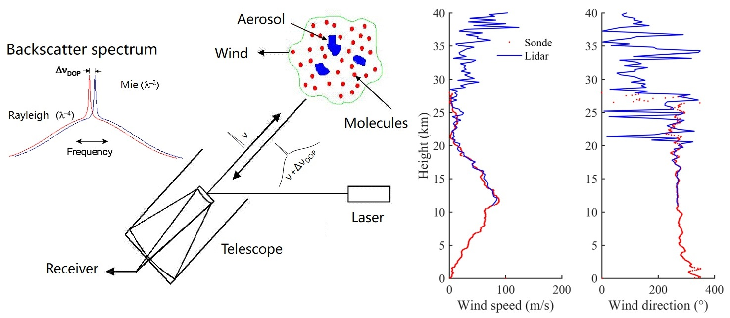
2.1. The Principle of Doppler Lidar
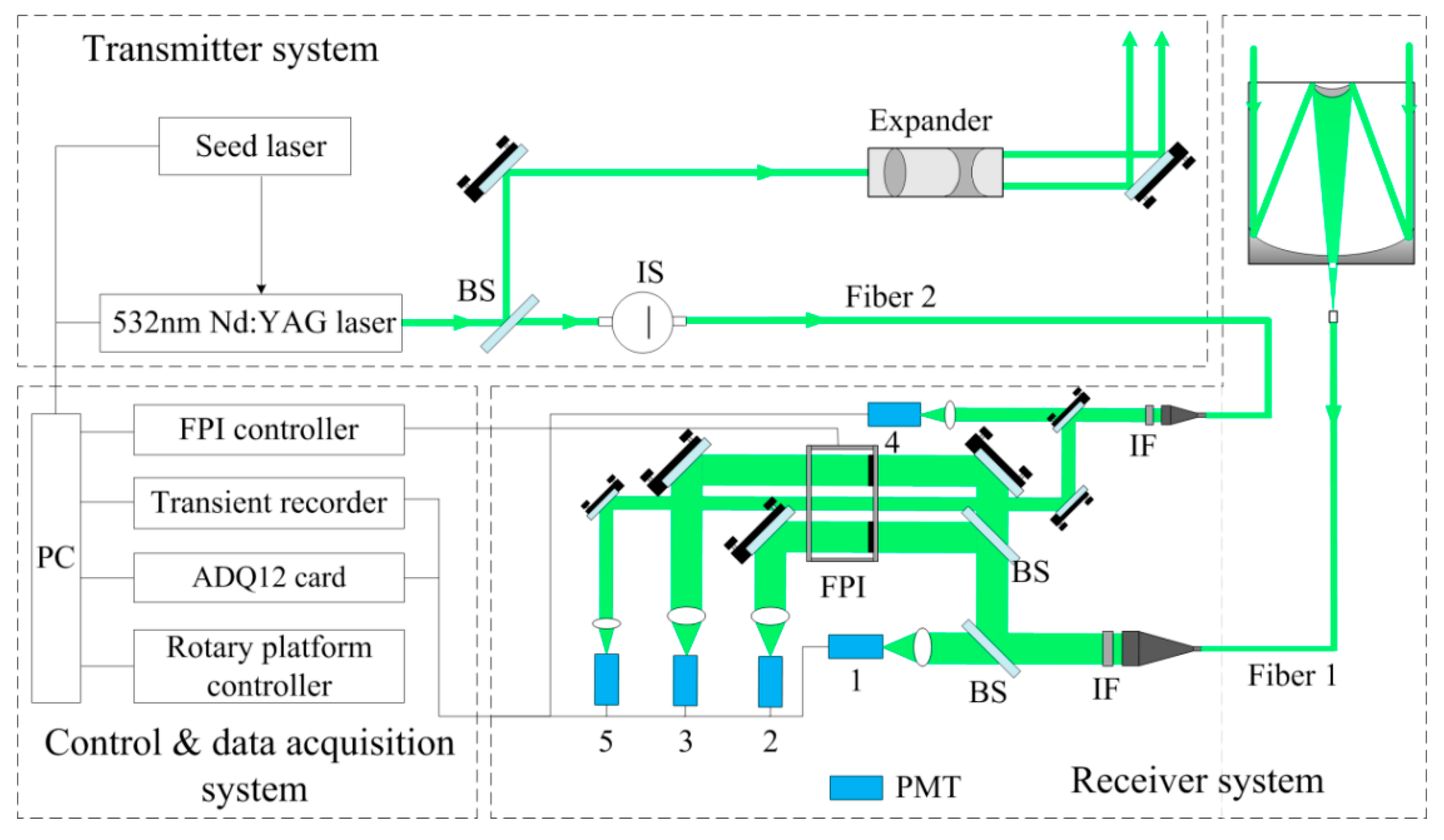
2.2. The Doppler Lidar System
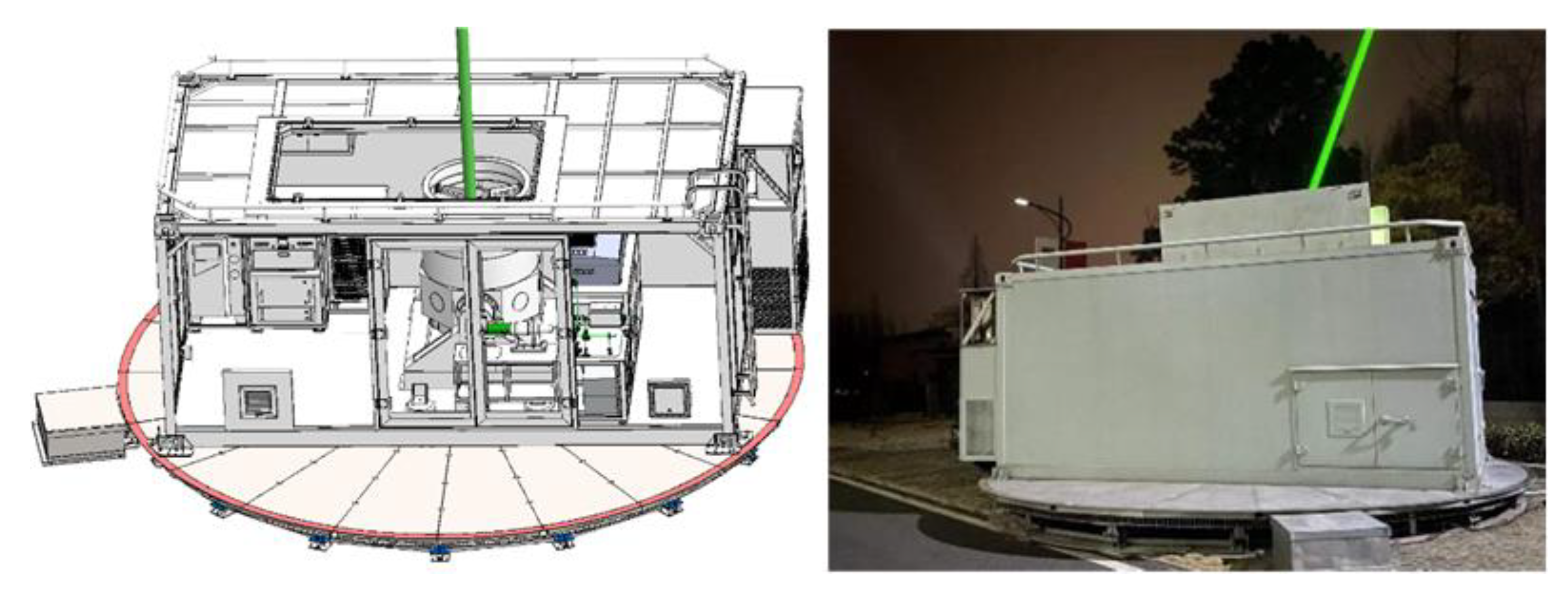
2.2.1. Structure and Parameters
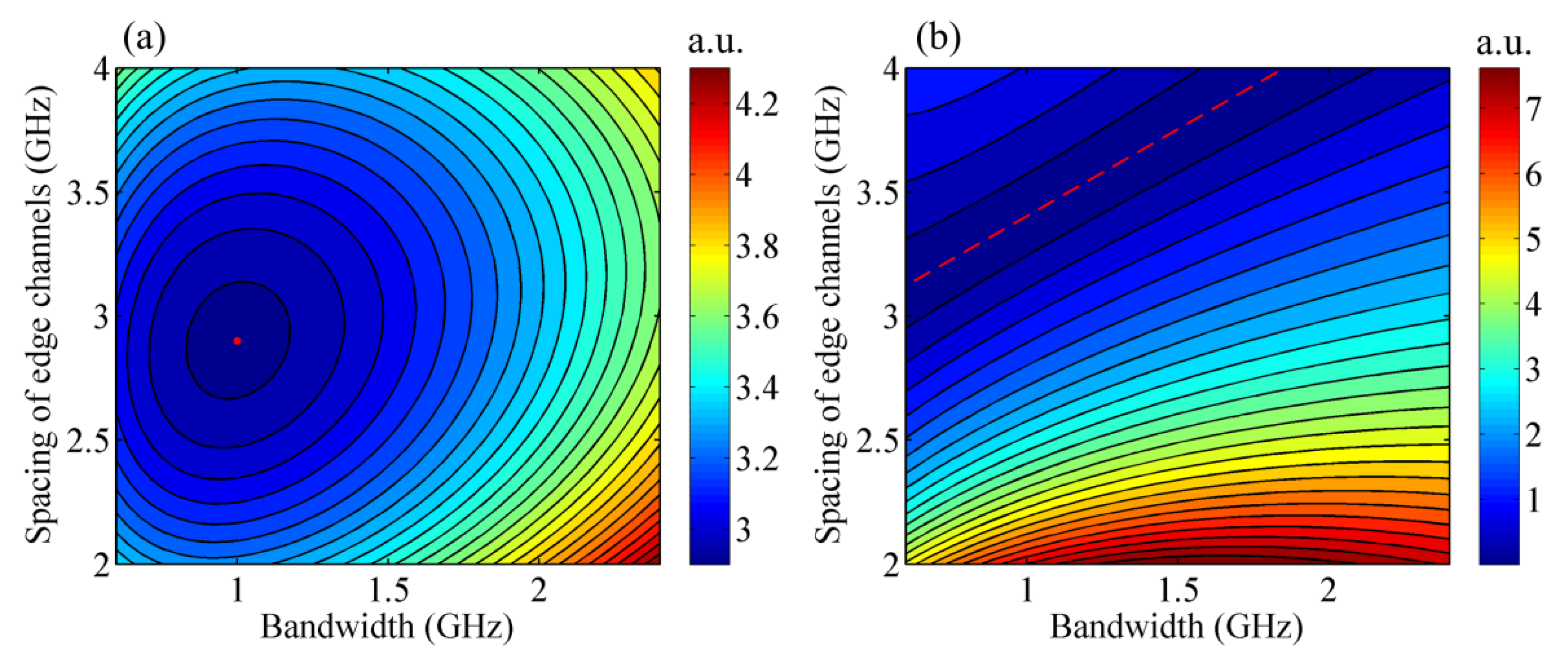
2.2.2. Design of the Fabry-Perot Interferometer
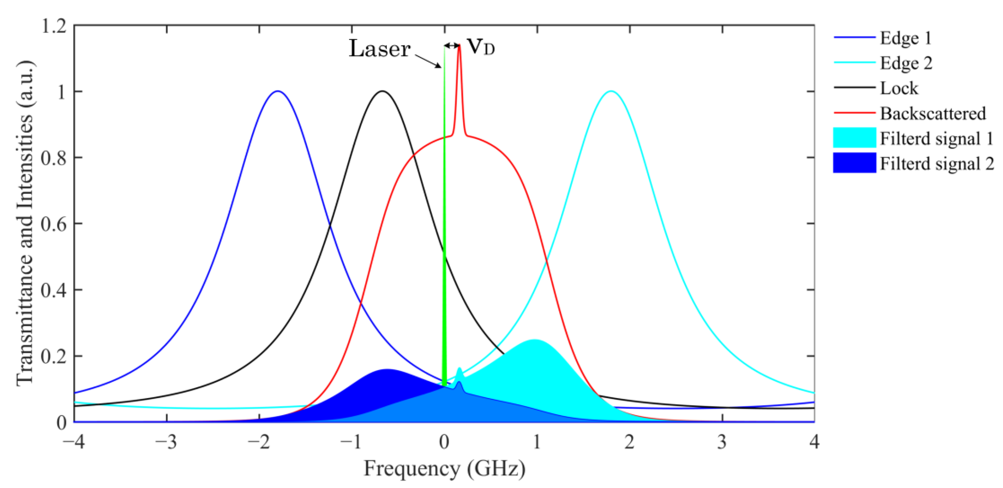
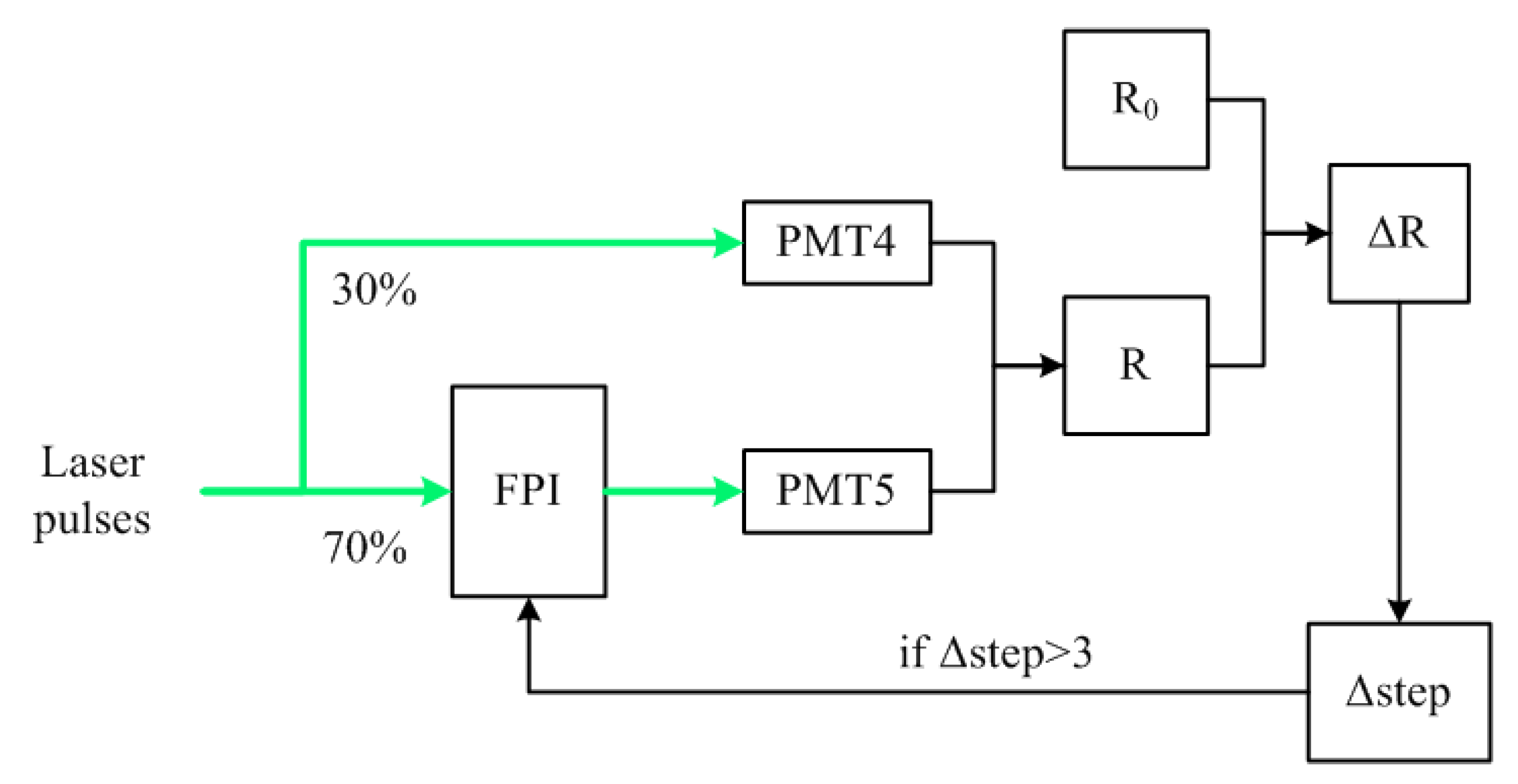
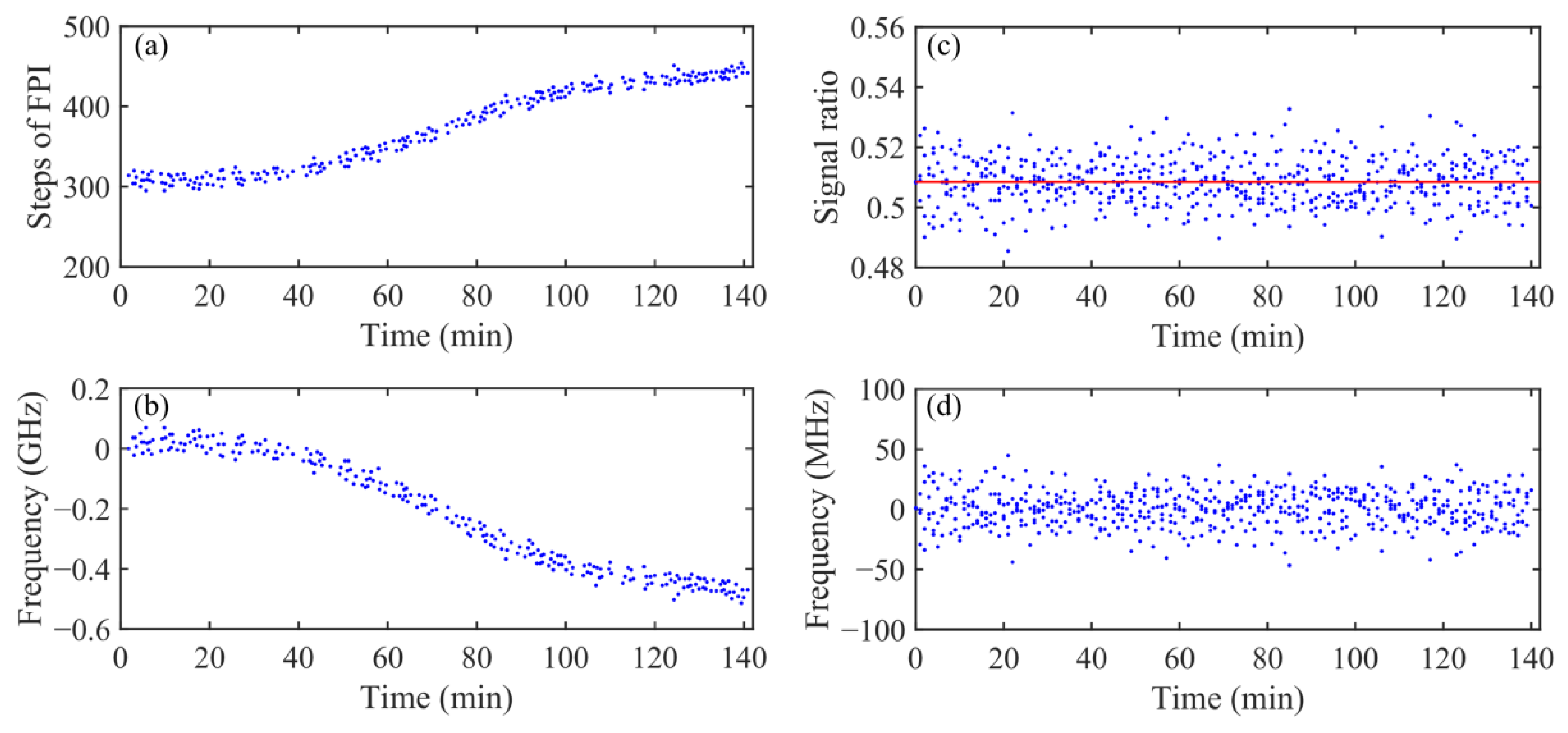
2.2.3. Frequency Locking of the FPI
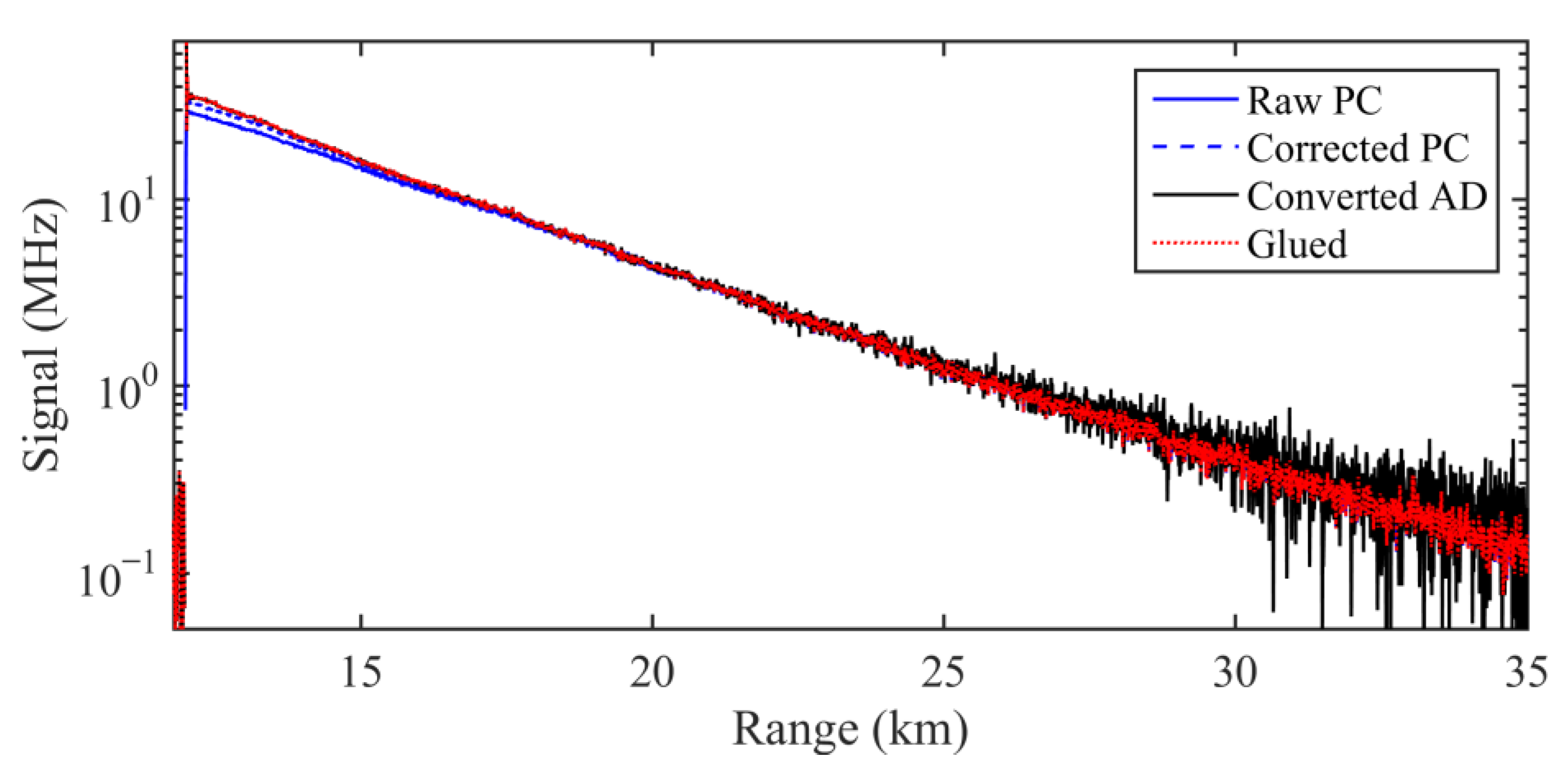
2.3. Signals Gluing
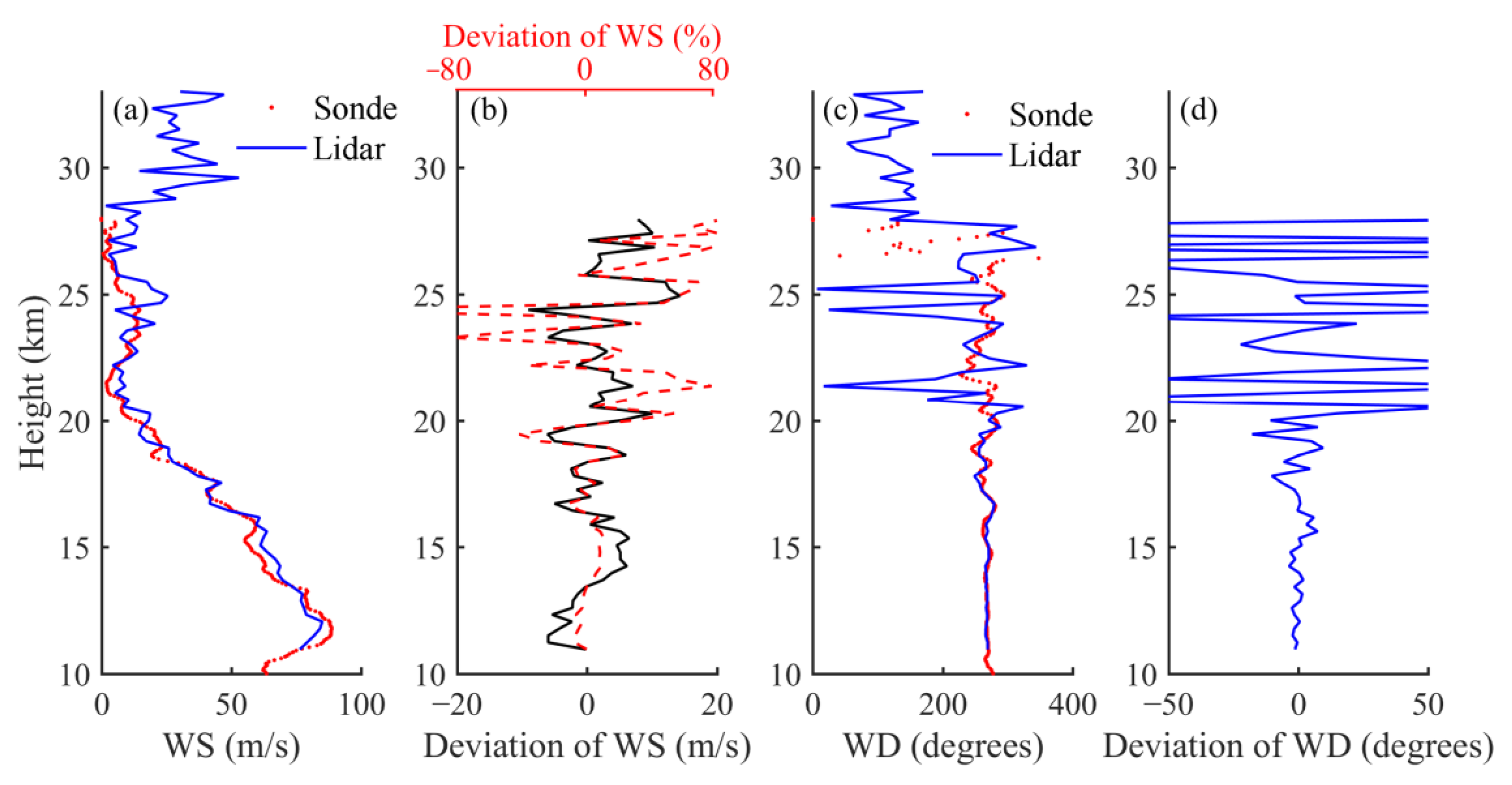
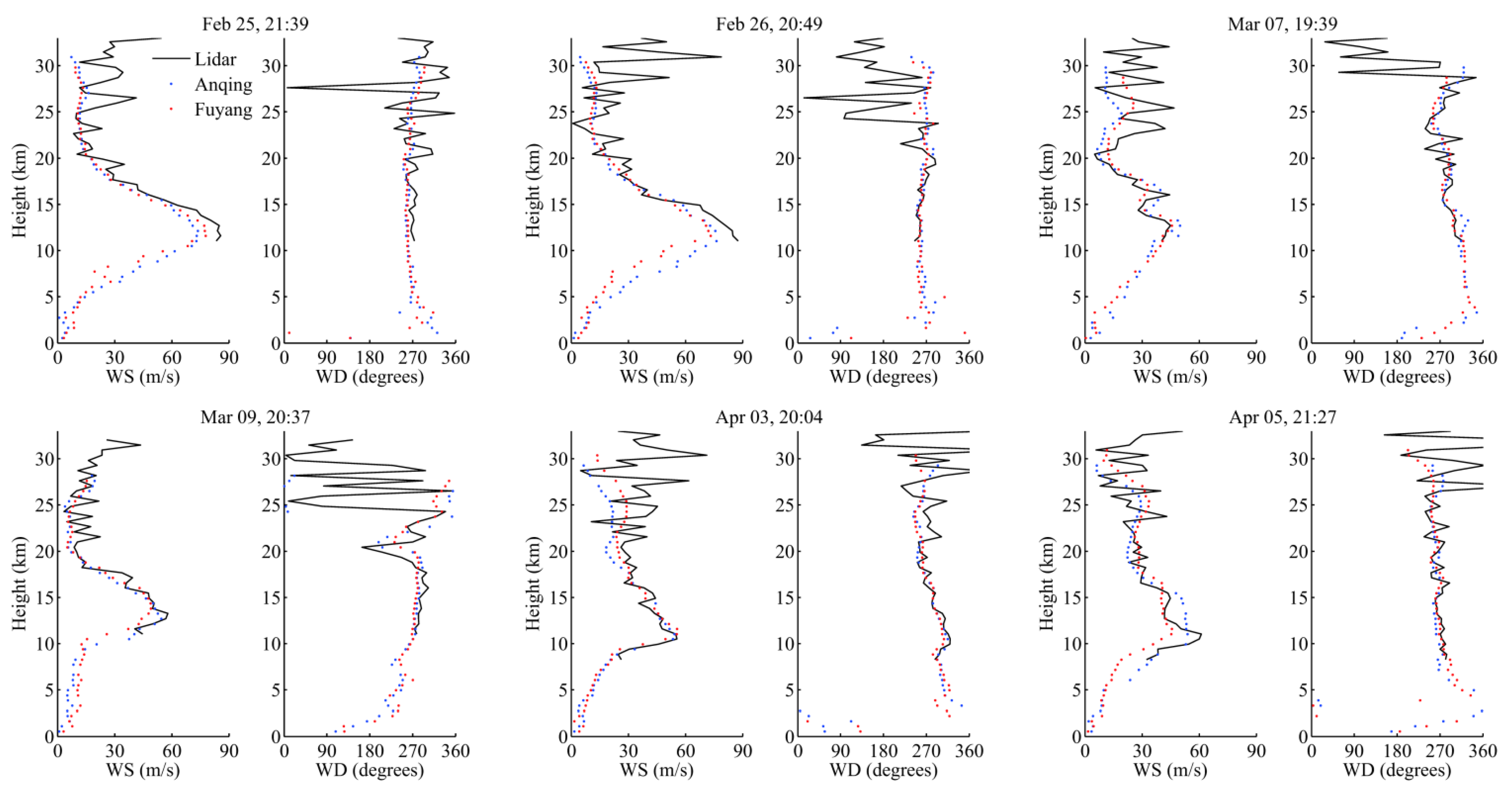
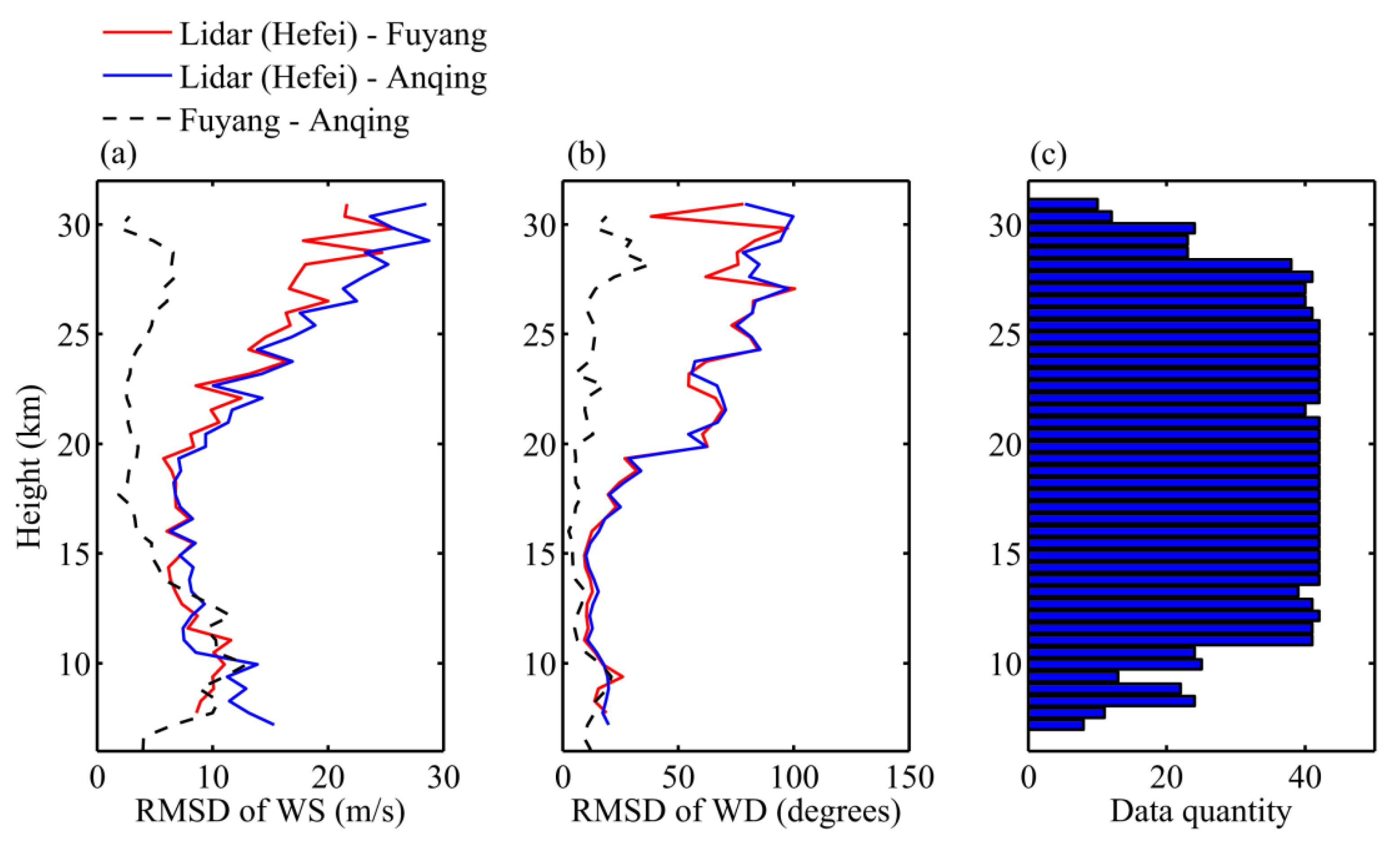
3. Results
4. Conclusions
Author Contributions
Funding
Data Availability Statement
Conflicts of Interest
References
- Yang, J.F.; Xiao, C.Y.; Hu, X.; Xu, Q. Responses of zonal wind at ~40°N to stratospheric sudden warming events in the stratosphere, mesosphere and lower thermosphere. Sci. China 2017, 60, 935–945. [Google Scholar] [CrossRef]
- Zhao, R.; Dou, X.; Xue, X.; Sun, D.; Han, Y.; Chen, C.; Zheng, J.; Li, Z.; Zhou, A.; Han, Y.; et al. Stratosphere and lower mesosphere wind observation and gravity wave activities of the wind field in China using a mobile Rayleigh Doppler lidar. J. Geophys. Res. Space Phys. 2017, 122, 8847–8857. [Google Scholar] [CrossRef]
- Hedin, A.E.; Fleming, E.L.; Manson, A.H.; Schmidlin, F.J.; Avery, S.K.; Clark, R.R.; Franke, S.J.; Fraser, G.J.; Tsuda, T.; Vial, F.; et al. Empirical wind model for the upper, middle and lower atmosphere. J. Atmos. Terr. Phys. 1996, 58, 1421–1447. [Google Scholar] [CrossRef]
- Prasad, N.S.; Sibell, R.; Vetorino, S.; Higgins, R.; Tracy, A. All-Fiber, Modular, Compact Wind Lidar for Wind Sensing and Wake Vortex Applications. Proc. SPIE 2015, 9465, 94650C. [Google Scholar]
- Lombard, L.; Valla, M.; Planchat, C.; Goular, D.; Augère, B.; Bourdon, P.; Canat, G. Eyesafe coherent detection wind lidar based on a beam-combined pulsed laser source. Opt. Lett. 2015, 40, 1030–1033. [Google Scholar] [CrossRef]
- Liu, H.; Zhu, X.; Fan, C.; Bi, D.; Liu, J.; Zhang, X.; Zhu, X.; Chen, W. Field Performance of All-Fiber Pulsed Coherent Doppler Lidar. Eur. Phys. J. Conf. 2020, 237, 08009. [Google Scholar] [CrossRef]
- Chanin, M.L.; Garnier, A.; Hauchecorne, A.; Porteneuve, J. A doppler lidar for measuring winds in the middle atmosphere. Geophys. Res. Lett. 1989, 16, 1273–1276. [Google Scholar] [CrossRef]
- Tepley, C.A.; Sargoytchev, S.I.; Hines, C.O. Initial doppler rayleigh lidar results from arecibo. Geophys. Res. Lett. 1991, 18, 167–170. [Google Scholar] [CrossRef]
- Korb, C.L.; Gentry, B.M.; Li, X.; Flesia, C. Theory of the double-edge technique for Doppler lidar wind measurement. Appl. Opt. 1998, 37, 3097–3104. [Google Scholar] [CrossRef]
- Gentry, B.M.; Chen, H. Tropospheric wind measurements obtained with the Goddard Lidar Observatory for Winds (GLOW): Validation and performance. Proc. SPIE 2002, 4484, 74–81. [Google Scholar]
- Dou, X.; Han, Y.; Sun, D.; Xia, H.; Shu, Z.; Zhao, R.; Shangguan, M.; Guo, J. Mobile rayleigh Doppler lidar for wind and temperature measurements in the stratosphere and lower mesosphere. Opt. Express 2014, 22, A1203–A1221. [Google Scholar] [CrossRef] [PubMed] [Green Version]
- Shangguan, M.; Xia, H.; Wang, C.; Qiu, J.; Shentu, G.; Zhang, Q.; Dou, X.; Pan, J. All-fiber upconversion high spectral resolution wind lidar using a Fabry-Perot interferometer. Opt. Express 2016, 24, 19322. [Google Scholar] [CrossRef] [PubMed]
- Xia, H.; Shangguan, M.; Wang, C.; Shentu, G.; Qiu, J.; Zhang, Q.; Dou, X.; Pan, J. Micro-pulse upconversion Doppler lidar for wind and visibility detection in the atmospheric boundary layer. Opt. Lett. 2016, 41, 5218–5221. [Google Scholar] [CrossRef] [Green Version]
- Liu, Z.; Liu, B.; Li, Z.; Yan, Z.; Wu, S.; Sun, Z. Wind measurements with incoherent Doppler lidar based on iodine filters at night and day. Appl. Phys. B 2007, 88, 327–335. [Google Scholar] [CrossRef]
- Wang, Z.; Liu, Z.; Liu, L.; Wu, S.; Liu, B.; Li, Z.; Chu, X. Iodine-filter-based mobile doppler lidar to make continuous and full-azimuth-scanned wind measurements: Data acquisition and analysis system, data retrieval methods, and error analysis. Appl. Opt. 2010, 49, 6960–6978. [Google Scholar] [CrossRef] [PubMed]
- Baumgarten, G. Doppler Rayleigh/Mie/Raman lidar for wind and temperature measurements in the middle atmosphere up to 80 km. Atmos. Meas. Tech. 2010, 3, 1509–1518. [Google Scholar] [CrossRef] [Green Version]
- Claude, S.; Anne, G.; Albert, H.; Hauchecorne, A.; Porteneuve, J. Rayleigh–mie doppler wind lidar for atmospheric measurements. 1. instrumental setup, validation, and first climatological results. Appl. Opt. 1999, 38, 2410–2421. [Google Scholar]
- Tenti, G.; Boley, C.D.; Desai, R.C. On the kinetic model description of rayleigh-brillouin scattering from molecular gases. Can. J. Phys. 1974, 52, 285–290. [Google Scholar] [CrossRef]
- Omote, K. Dead-time effects in photon counting distributions. Nucl. Instrum. Methods Phys. Res. 1990, A293, 582–588. [Google Scholar] [CrossRef]
- Donovan, D.P.; Whiteway, J.A.; Carswell, A.I. Correction for nonlinear photon counting effects in lidar systems. Appl. Opt. 1993, 32, 6742–6753. [Google Scholar] [CrossRef]
- Liu, Z.; Li, Z.; Liu, B.; Li, R. Analysis of saturation signal correction of the troposphere lidar. Chin. Opt. Lett. 2009, 7, 1051–1054. [Google Scholar] [CrossRef]
- Whiteman, D.N.; Melfi, S.H.; Ferrare, R.A. Raman lidar system for the measurement of water vapor and aerosols in the Earth’s atmosphere. Appl. Opt. 1992, 31, 3068–3082. [Google Scholar] [CrossRef] [PubMed]
- Feng, C.; Wu, S.; Liu, B. Gluing Method of Detected Signal Based on Lidar. Acta Photonica Sin. 2018, 47, 0601101. (In Chinese) [Google Scholar]


| Measurement Performance | |
|---|---|
| Observation range | 10–35 km |
| Height resolution | 0.275–1.1 km (changeable) |
| Time resolution | 30 min (changeable) |
| Transmitter | |
| Laser wavelength | 532.1 nm |
| Pulse energy | 350 mJ |
| Repetition rate | 30 Hz |
| Spectral bandwidth (FWHM) | 70 MHz |
| Divergence angle | 50 μrad |
| Receiver | |
| Telescope diameter | 800 mm |
| FOV | 100 μrad |
| IF bandwidth (FWHM) | 0.3 nm |
| Fiber core diameters | 200 μrad (fiber 1) 100 μrad (fiber 2) |
| Fiber N.A. | 0.22 |
| Beam divergence | 2.5 mrad |
| Data acquisition | |
| Transient recorder | 12 bit, 20 MHz sampling rate |
| Acquisition card | 12 bit, 1 GHz sampling rate |
Publisher’s Note: MDPI stays neutral with regard to jurisdictional claims in published maps and institutional affiliations. |
© 2022 by the authors. Licensee MDPI, Basel, Switzerland. This article is an open access article distributed under the terms and conditions of the Creative Commons Attribution (CC BY) license (https://creativecommons.org/licenses/by/4.0/).
Share and Cite
Zhao, M.; Xie, C.; Wang, B.; Xing, K.; Chen, J.; Fang, Z.; Li, L.; Cheng, L. A Rotary Platform Mounted Doppler Lidar for Wind Measurements in Upper Troposphere and Stratosphere. Remote Sens. 2022, 14, 5556. https://doi.org/10.3390/rs14215556
Zhao M, Xie C, Wang B, Xing K, Chen J, Fang Z, Li L, Cheng L. A Rotary Platform Mounted Doppler Lidar for Wind Measurements in Upper Troposphere and Stratosphere. Remote Sensing. 2022; 14(21):5556. https://doi.org/10.3390/rs14215556
Chicago/Turabian StyleZhao, Ming, Chenbo Xie, Bangxin Wang, Kunming Xing, Jianfeng Chen, Zhiyuan Fang, Lu Li, and Liangliang Cheng. 2022. "A Rotary Platform Mounted Doppler Lidar for Wind Measurements in Upper Troposphere and Stratosphere" Remote Sensing 14, no. 21: 5556. https://doi.org/10.3390/rs14215556