Applying Deep Learning in the Prediction of Chlorophyll-a in the East China Sea

Abstract

The ocean chlorophyll-a (Chl-a) concentration is an important variable in the marine environment, the abnormal distribution of which is closely related to the hazards of red tides. Thus, the accurate prediction of its concentration in the East China Sea (ECS) is greatly important for preventing water eutrophication and protecting the coastal ecological environment. Processed by two different pre-processing methods, 10-year (2011–2020) satellite-observed chlorophyll-a data and logarithmic data were used as the long short-term memory (LSTM) neural network training datasets in this study. The 2021 data were used for comparison to prediction results. The past 15 days’ data were used to predict the concentration of chlorophyll-a for the five following days. Results showed that the predictions obtained by both pre-processing methods could simulate the seasonal distribution of the Chl-a concentration in the ECS effectively. Moreover, the prediction performance of the model driven by the original values was better in the medium- and low-concentration regions. However, in the high-concentration region, the prediction of extreme concentrations by the two data-driven LSTM models showed underestimation, considering that the prediction performance of the model driven by the original values was better. Results of sensitivity experiments showed that the prediction accuracy of the model decreased considerably when the backward prediction time step increased. In this study, the neural network was driven only by chlorophyll-a, whose concentration in the ECS was forecasted, and the effect of other relevant marine elements on Chl-a was not considered, which is the current weakness of this study.

1. Introduction

In marine ecosystems, marine phytoplankton chlorophyll-a (Chl-a) can effectively reflect the biomass of marine primary producers and the photosynthetic carbon sequestration capacity of marine primary productivity [1,2,3,4,5], which are fundamental to marine ecosystems. The prediction of the marine chlorophyll-a concentration and the analysis of its spatial and temporal changes are not only useful for the study of marine primary productivity, but also important for the study of carbon cycling in the ocean–atmosphere system [6,7], red tide hazard monitoring [8,9,10], environmental monitoring [11], ocean currents (such as upwelling and coastal currents) [12,13], as well as fishery management and the estimation of aquaculture production [14].

The chlorophyll-a concentration is influenced by many factors, such as climatic factors, namely light, temperature, precipitation, and wind speed [15,16], and geographical factors [17,18]. In addition, in the early period, a relative paucity of data relating to the Chl-a concentration was observed, leading to a high level of uncertainty in its prediction. The prediction methods could be broadly categorized into two methods. The first is the statistical method, which was first proposed by Vollenweider [19], who used statistical models to predict the issue of eutrophication. Kiyofuji et al. [20] developed a statistical spatiotemporal model to predict the distribution of chlorophyll-a in the Sea of Japan on the basis of SeaWiFS data. Although the model was able to predict its distribution effectively during summer and early autumn, this traditional statistical method could only solve the average concentration of a particular element and could not simulate the effect of relevant factors on chlorophyll-a. The second method is based on ecological dynamics, the properties of water bodies, and establishing a theoretical analysis model to predict the concentration of chlorophyll-a [21,22,23]. Using data collected monthly, Liu et al. [24] used multivariate statistical methods to simulate the effects of multiple chemical variables on chlorophyll-a in Lake Qilu. This method considers the interactions between elements in nature and includes many parameters, thereby causing difficulty in accurate modeling or parameterization due to the diversity of water quality variables in the ocean.

The research on remote sensing monitoring of chlorophyll-a and remote sensing inversion has become increasingly sophisticated with the development of satellite remote sensing technology. Moreover, a large amount of water quality data can be obtained as the access to information becomes more diverse. A new trend in recent years has been the use of machine learning methods for water quality variable prediction. Machine learning methods can capture the characteristics of the input data to explore the potential relationships between variables, and narrow the difference between predictions and observations by updating the parameters in the model. The most widely used machine learning methods at present include artificial neural networks (ANN, [25,26,27,28,29]), support vector machine (SVM, [30,31,32]), decision tree (DT), random forest (RF, [32,33,34,35]), and regression, etc. Deep learning (DL) is a special type of machine learning [36]. Zhang et al. [37] proposed a new prediction approach for algal blooms on the basis of deep learning to represent and predict highly dynamic and complex phenomena. Most current studies use independent deep learning models for chlorophyll-a concentration prediction. Several deep learning models, such as the recurrent neural network (RNN) and its variant, the long short-term memory neural network (LSTM), are commonly used in time-series forecasting. Both approaches have good performance in dealing with time-series information problems. Compared with the traditional RNN, LSTM does not have the problem of gradient disappearance in the process of training long-term sequences. Therefore, the LSTM model can effectively predict the chlorophyll-a concentration [38,39,40]. Yossof et al. [41] used an LSTM model and a convolutional neural network (CNN) model to predict harmful algal blooms on the western coast of Sabah. The results show that the LSTM model outperforms the CNN model in terms of prediction accuracy. Barzegar et al. [42] first built a coupled CNN–LSTM model to predict water quality variables in Small Prespa Lake, Greece, and the results showed that the hybrid CNN–LSTM model was better than the independent model in predicting the chlorophyll-a concentration.

The Eastern China Sea (ECS) area is under the influence of the East Asian monsoon; the chlorophyll-a concentration in the ECS has evident seasonal variation characteristics and is influenced by land runoff, mainly from the Yangtze River [43,44,45]. The distribution of it in the East China Sea is also influenced by the Kuroshio, with high-temperature and high-salt seawater [46,47]. The Eastern China Sea area has a long coastline, of which the Zhejiang coast is one of the famous upwelling areas in China, and it has important fishing grounds, such as the Zhoushan and Yushan fishing grounds [48]. With the rapid development of coastal cities in recent years, the frequency of red tides in the ECS has increased substantially [14,49], not only polluting the marine environment of this region but also severely damaging the fishery resources, leading to huge economic losses [50]. Therefore, accurate prediction of the chlorophyll-a concentration in this area is important for the prevention of eutrophication and the protection of the offshore ecosystem.

Machine learning methods have been applied to research on forecasting ocean elements, such as storm surges [51], harmful algal blooms (HAB), and sea surface temperature (SST) in the ECS. Xu et al. [52] used the SVM model to predict the occurrence of red tides in Haizhou Bay in the ECS. Xiao et al. [53,54] used a combined LSTM–AdaBoost model and a convolutional LSTM (ConvLSTM) model to predict the SST field in the ECS, respectively. The results showed that the LSTM–AdaBoost and ConvLSTM models have good promise in accurately predicting the short- and medium-term SST fields.

At present, no research has used machine learning to predict the chlorophyll-a concentration in the East China Sea area. Thus, this study first uses the LSTM neural network to predict the concentration in this region. The specific objectives of this research are (1) comparing the effects of different processing methods for chlorophyll-a data on the forecast result; and (2) evaluating the prediction results of the LSTM neural network in the ECS on the basis of the previous step by using the optimal processing method for chlorophyll-a data.

The rest of this paper is organized as follows, Section 2 describes the satellite data and LSTM neural network used in this study, Section 3 presents the experimental results and detailed discussion, and Section 4 draws the conclusions obtained from this study.

2. Materials and Methods

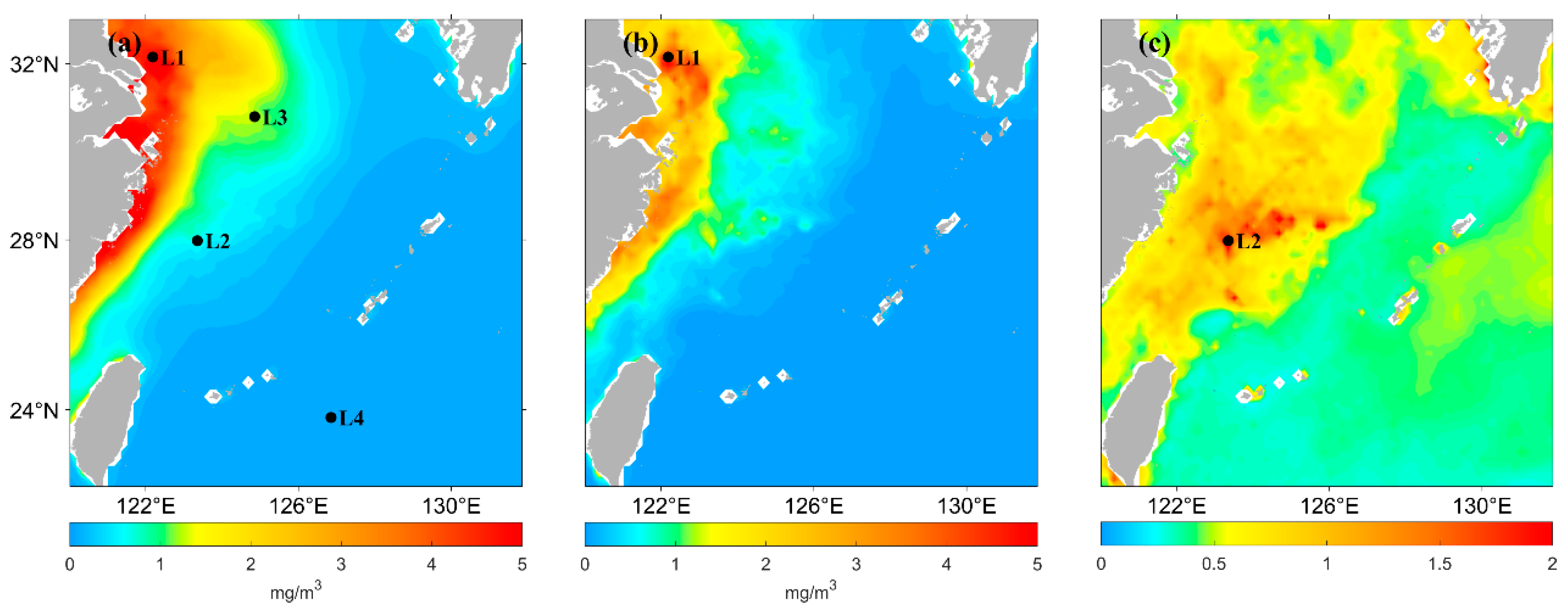
2.1. Materials

This study uses the ocean color data product (OCEANCOLOUR_GLO_BGC_L4_MY_009_104) provided by the Copernicus Marine Environment Monitoring Service (CMEMS, http://www.copernicus.eu/ (accessed on 11 July 2022)). This product integrates data from SeaWiFS, MODIS-Aqua, MODIS-Terra, MERIS, VIIRS-SNPP, OLCI-S3A&S3B, and other satellites. The time resolution is 1 day, the spatial resolution is 4 km × 4 km, and the time span is from September 1997 to the present. The spatial range of chlorophyll-a data used in our study is 22°N–33°N, 120°E–131°E, and the time range is from 2011 to 2021, of which the data from 2011 to 2020 are used as the training dataset, and the chlorophyll-a data from 2021 are used as the test dataset.

2.2. Methods

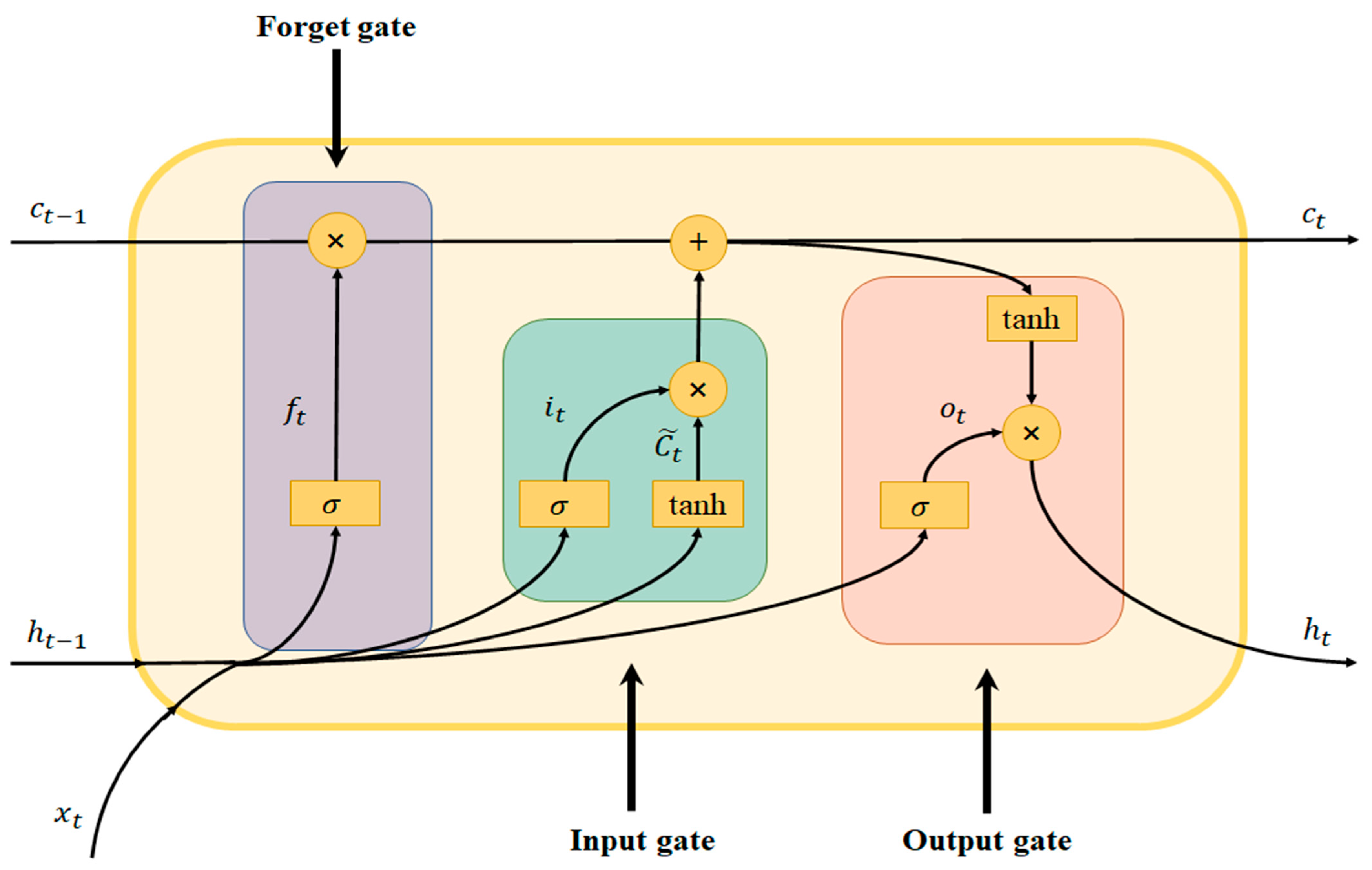
2.2.1. LSTM Neural Network

LSTM was proposed by Hochreiter and Schmidhuber in 1997 [55] as a variant neural network of RNN for long-time-series training. It can effectively solve the gradient disappearance problem, which easily occurs in the training process of the traditional RNN. The internal network structure of the LSTM unit is more complex than that of the traditional RNN. The information in the current unit is processed by the input gate, forgetting gate, and output gate, and then the historical unit information is selected to be either “forgotten” or “remembered”.

The two most important states in the LSTM cell structure are the cell state $c\left(t\right)$ and the hidden state $h\left(t\right)$. The cell state transmits information through different gates, thereby enhancing the dependency among long-time-series information; the cell structure is shown in Figure 1.

First, the function of the forget gate $f_t$ is to select which information needs to be discarded in the current state of the cell. $f_t$ is calculated as follows:

$$f_t=\sigma \left(W_{fh}{h}_{t-1}+W_{fx}{x}_t+b_f\right)$$

(1)

where $\sigma (\cdot )$ represents the sigmoid activation function, $W_{fh}$ and $W_{fx}$ represent the corresponding weight parameters, $x_t$ represents the input at moment $t$, $h_{t-1}$ represents the hidden state of the cell at moment $t-1$, and $b_f$ is the bias term.

Second, the function of the input gate $i_t$ is to remember the candidate cell state selectively, thereby updating the cell state at the current moment, and a new cell state $\widetilde{C_t}$ is generated by the following calculation formula:

$$i_t=\sigma \left(W_{ih}{h}_{t-1}+W_{ix}{x}_t+b_i\right)$$

(2)

$$\widetilde{C_t}=\tanh \left(W_{ch}{h}_{t-1}+W_{cx}{x}_t+b_c\right)$$

(3)

$$C_t=f_t\times C_{t-1}+i_t\times \widetilde{C_t}$$

(4)

where $\sigma (\cdot )$ represents the sigmoid activation function; $W_{ih}$, $W_{ix}$, $W_{ch}$, and $W_{cx}$ represent the corresponding weight parameters, $x_t$ represents the input at moment $t$, $h_{t-1}$ represents the hidden state of the cell at moment $t-1$, $\widetilde{C_t}$ represents the candidate state at the current moment, and $b_i$ and $b_c$ are bias terms.

Then, the output gate $o_t$ is used to determine the output component of the cell state through the sigmoid function, whereas the cell state is processed through tanh and multiplied with the output gate $o_t$ to obtain the new hidden state $h_t$; the calculation formula is as follows:

$${\sigma }_t=\sigma \left(W_{oh}{h}_{t-1}+W_{ox}{x}_t+b_o\right)$$

(5)

$$h_t=o_t\times \tanh \left(c_t\right)$$

(6)

where $\sigma (\cdot )$ represents the sigmoid activation function, $W_{oh}$ and $W_{ox}$ represent the corresponding weight parameters, $x_t$ represents the input at moment $t$, and $b_o$ represents the bias term.

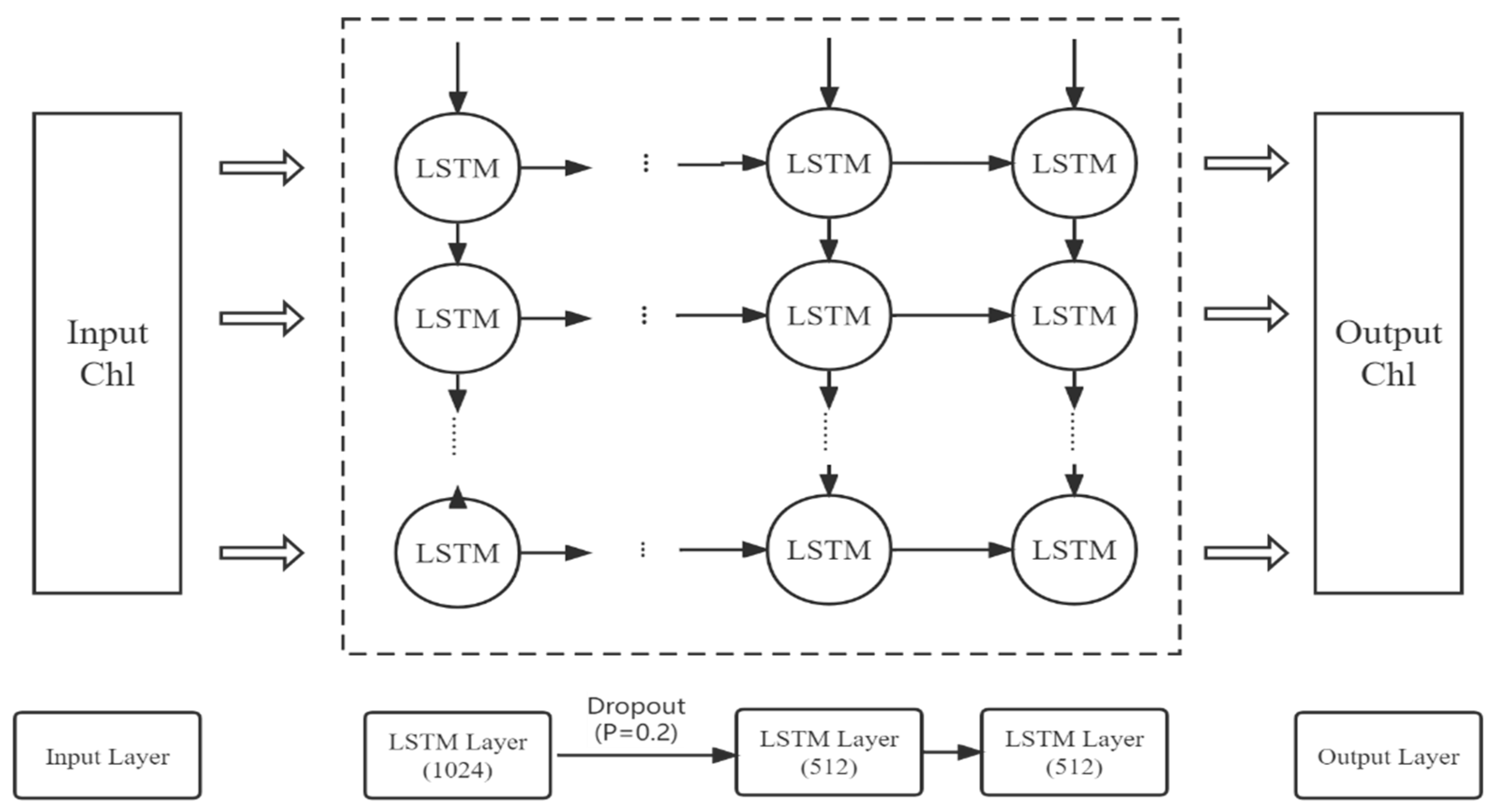
2.2.2. Architecture of the LSTM Model for Chl-a Forecasts

In this study, a regional chlorophyll-a concentration prediction model is established on the basis of the LSTM neural network, including an input layer, three LSTM layers, a dropout layer, and a dense layer, as shown in Figure 2. Dropout is a method to control the complexity of the model. In each training batch, a certain number of hidden nodes are set to 0 to reduce the interaction between hidden nodes, thereby preventing the model from overfitting [56,57]. During training, we use tanh as the activation function to generate the output of hidden neurons. Adam optimization is a stochastic gradient descent method based on the adaptive estimation of first- and second-order moments; compared with other stochastic optimization algorithms, the Adam algorithm has more advantages in practical applications [58]. Therefore, in this study, we adopt the Adam optimization algorithm to minimize the error between predicted and observed values.

2.2.3. Data Pre-Processing

To investigate the effect of different input data on the prediction results of the LSTM model, one group used the original data as input to the model, and the other group used the logarithmic data as input to the LSTM model. Both groups used the data of the previous 15 days to predict the value of the next 5 days. Data from 2011 to 2020 were used to generate the corresponding training and validation datasets, where the ratio of the data volume of the training dataset to the validation dataset was 4:1. Data from 2021 were used as a test dataset to make predictions for chlorophyll-a, which was excluded from the model training to ensure relative independence between the training and test datasets. To explore the influence of input length on the prediction results of the LSTM model, under the condition that hyperparameters, such as the number of hidden layers, the neurons, and the learning rate, do not change, the prediction length was controlled to 1 day, and the input length was set to 7, 10, and 15 days, respectively. Similarly, to explore the influence of the prediction length on the prediction results of the model when the other hyperparameters remain unchanged, the input length was controlled to 15 days, and the prediction length was set to 1, 3, and 5 days, respectively. The training dataset used in the training model needed to be standardized. In the process of standardizing the data, we used the MinmaxScaler function imported from the sklearn library to scale the data of the training dataset to (−1, 1) to obtain the standardized training dataset.

2.2.4. Evaluation Functions

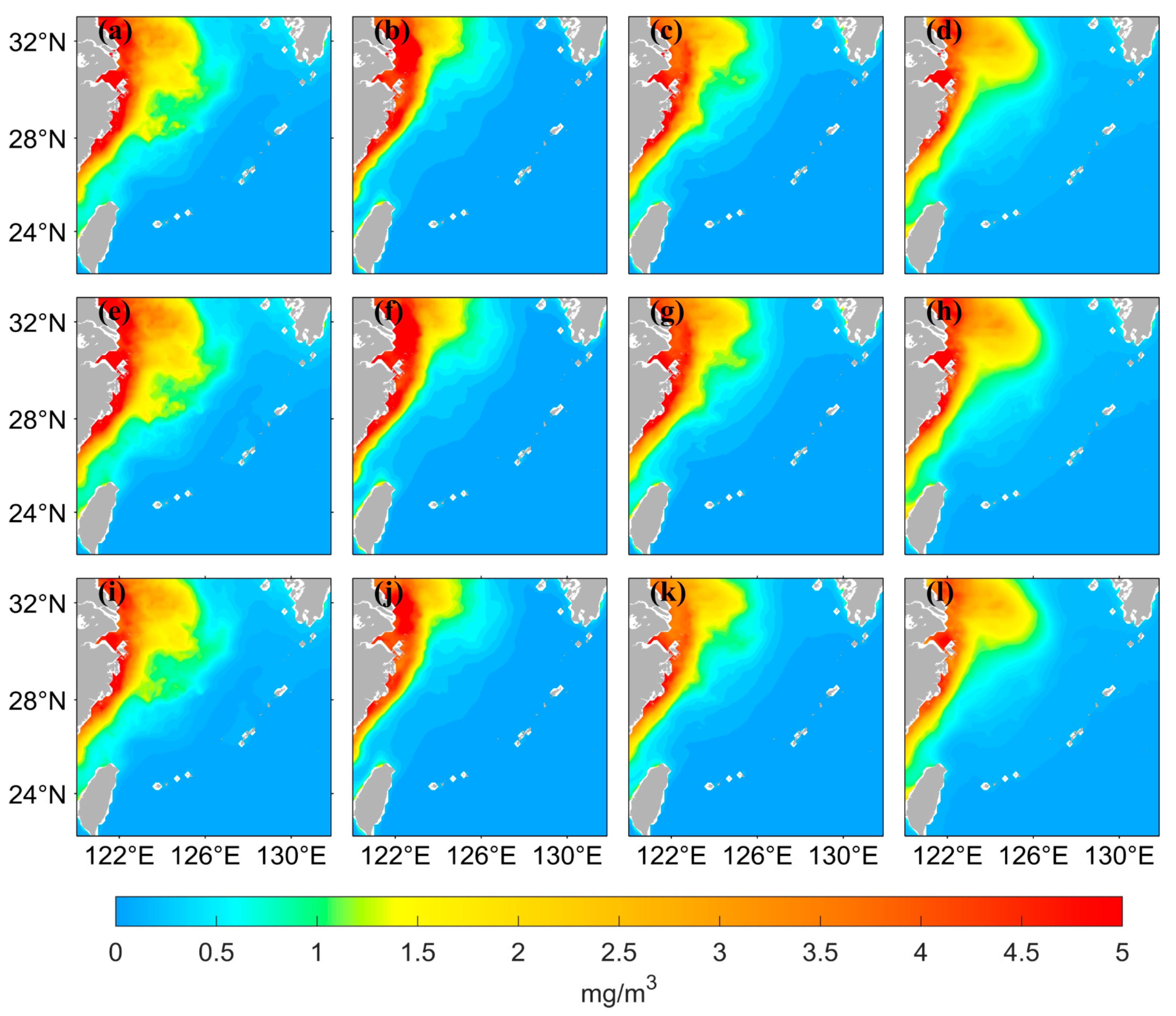
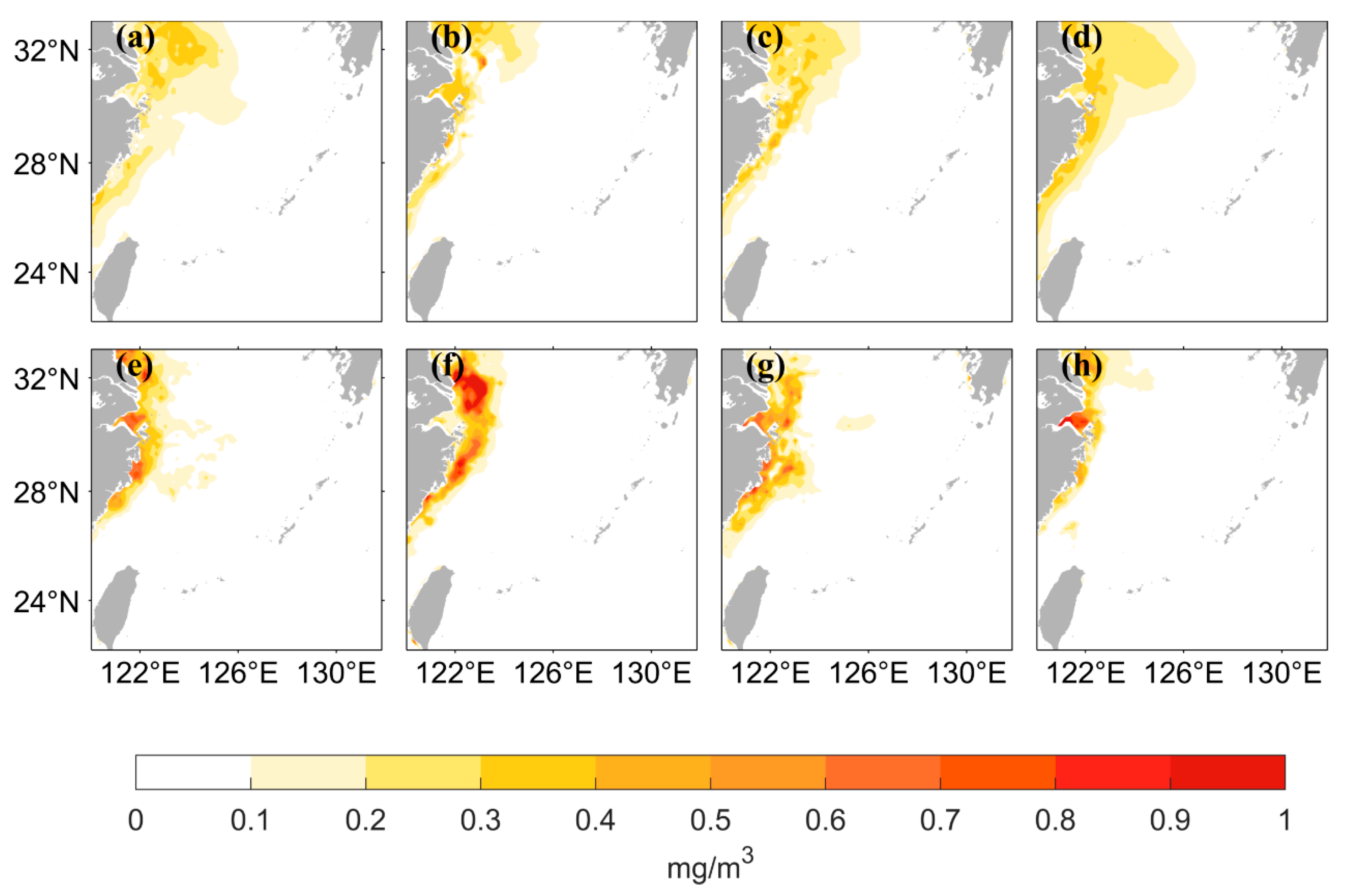
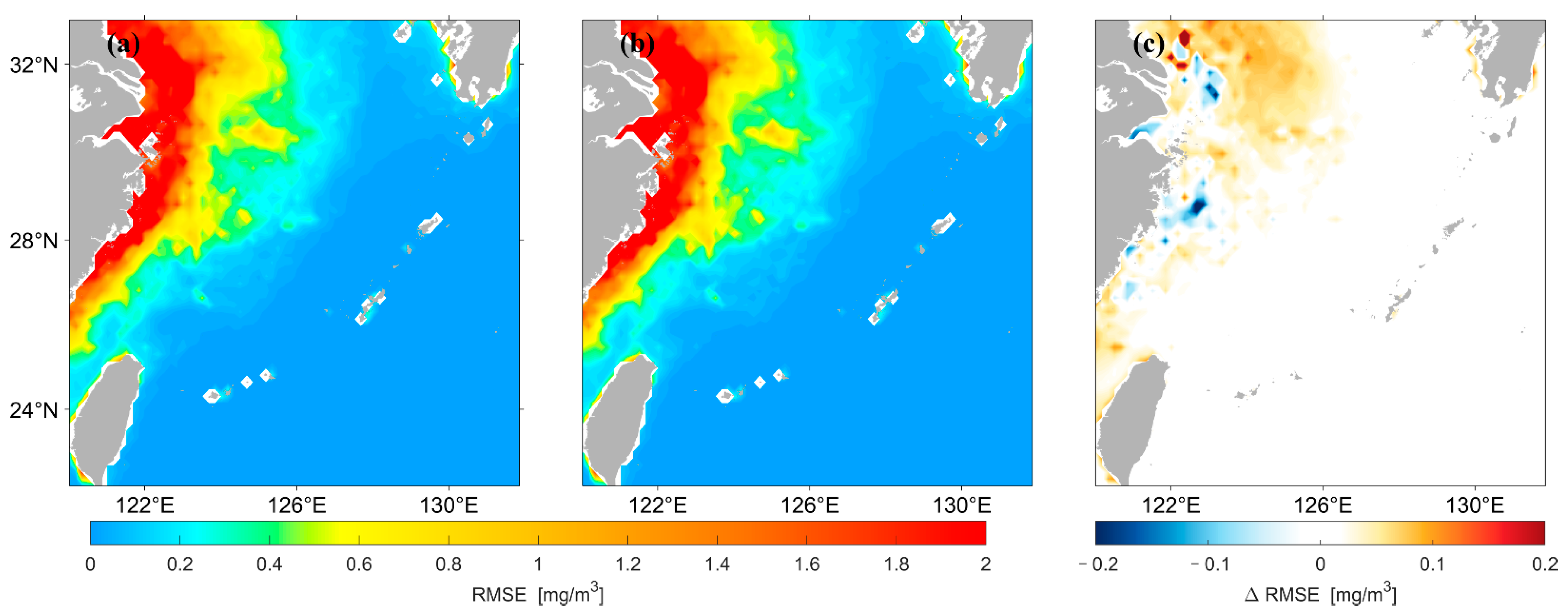
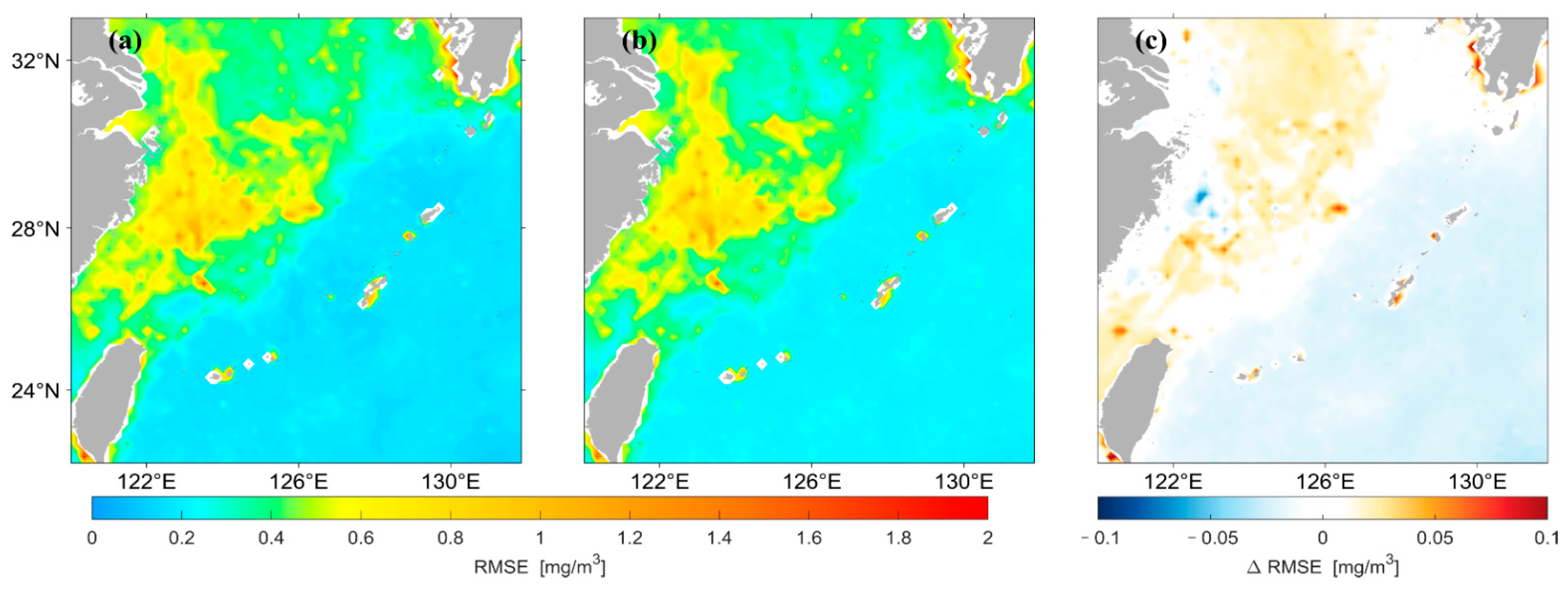
To compare the performance of the different methods further, the following indicators were used in this study to evaluate model performance: root mean square error ($RMSE$), standard deviation ($STD$), coefficient of determination ($R^2$), and absolute error ($AE$). The formulas are shown below.

$$RMSE=\sqrt{\frac{1}{n}{{\displaystyle \sum }}_{t=1}^n{\left(Y_t-y_t\right)}^2}$$

(7)

$$S=\sqrt{\frac{{{\displaystyle \sum }}_{t=1}^n{\left(x_t-\overline{x}\right)}^2}{n-1}}$$

(8)

$$R^2=1-\frac{{{\displaystyle \sum }}_{t=1}^n\left(Y_t-y_t\right)}{\sqrt{{{\displaystyle \sum }}_{t=1}^n{\left(Y_t-\overline{Y}\right)}^2}}$$

(9)

$$AE=\left|Y_t-y_t\right|$$

(10)

where $Y$ represents the satellite-observed value, $\overline{Y }$ represents the average of the satellite-observed values, $y$ represents the model-predicted value, and $y$ represents the average of the model-predicted chlorophyll-a values. $x$ represents the value from satellite observations or model forecasts, and $\overline{x}$ represents the average of the values from satellite observations or model forecasts. Small $RMSE$ and $AE$ values indicate the high forecast accuracy of the model. The closer the value of $S$ to the $STD$ of the observed values, the better the prediction performance of the model. The closer the value of $R^2$ to 1, the higher the fitness between the predicted and observed values.

3. Results

The chlorophyll-a concentration in the East China Sea varies widely from nearshore to offshore due to the influence of surface runoff. It also has substantial seasonal variations due to environmental factors, such as monsoons and ocean currents. Therefore, this study selected four points, marked as L1 (32.1°N, 122.2°E), L2 (28.0°N, 123.4°E), L3 (30.8°N, 124.9°E), and L4 (23.8°N, 126.9°E), as shown in Figure 3, to analyze the chlorophyll-a concentration predicted by the LSTM model. L1 was selected because the annual mean of the chlorophyll-a concentration at this location is higher, as well as the standard deviation of the concentration. L2 and L3 were selected because these points are located in the median area of the annual mean chlorophyll-a concentration; the coefficient of chlorophyll-a variation is higher at L2. L4 was selected because the concentration in location L4 is lower in the distant sea area.

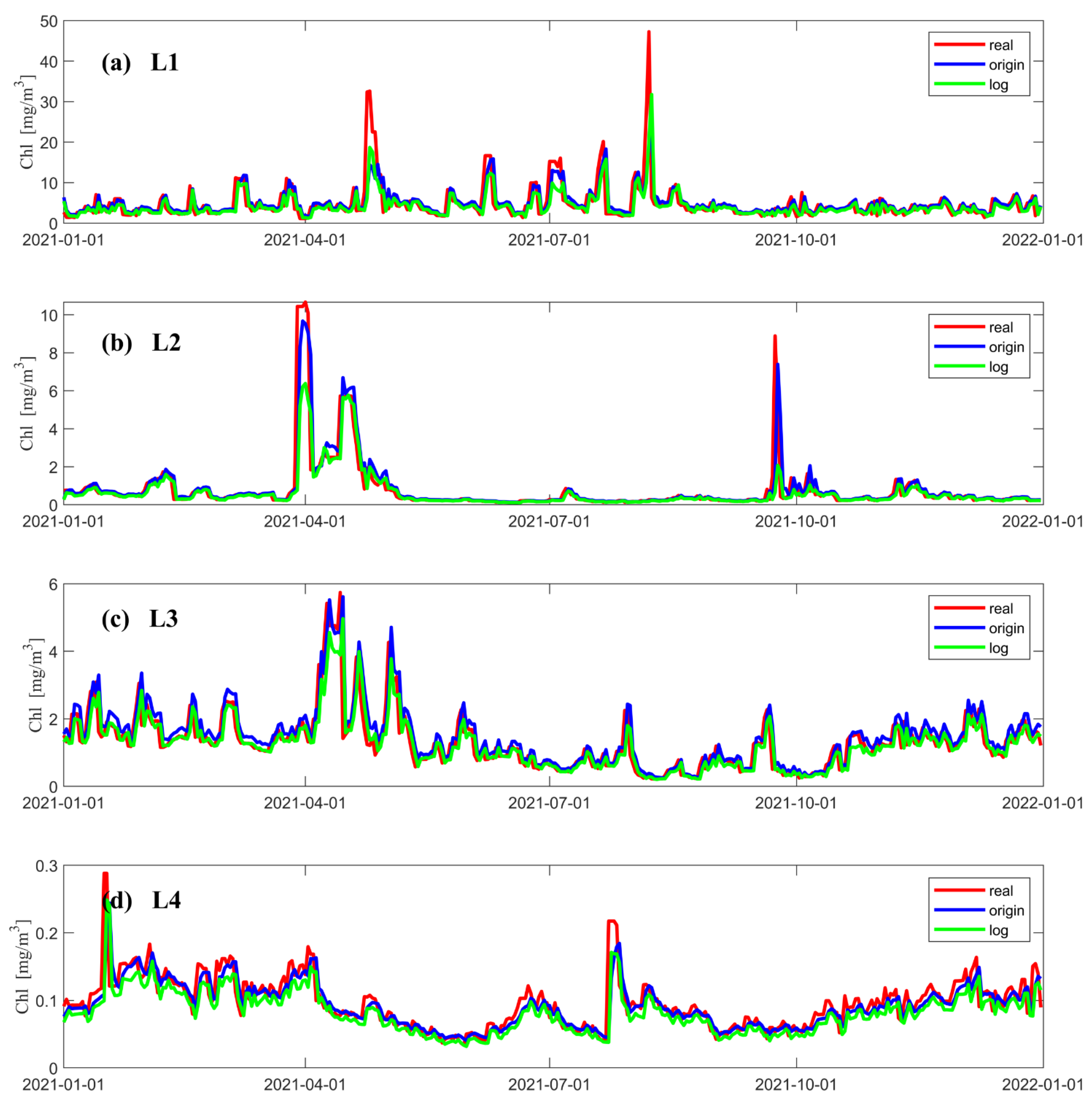
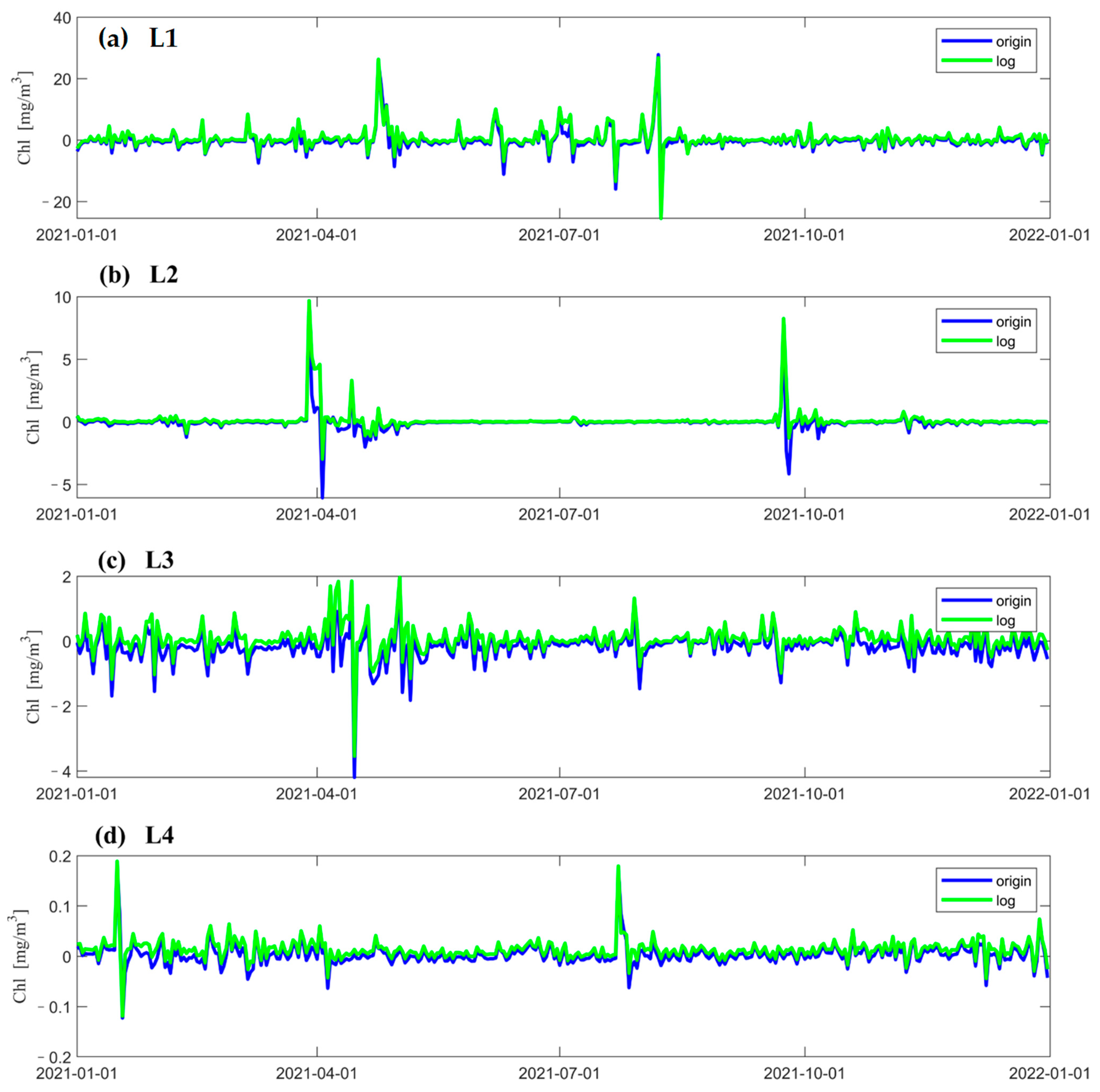
3.1. LSTM Prediction Results under Different Data Pre-Processing Methods

First, this study discussed the effect of chlorophyll-a data obtained from different data pre-processing methods on the prediction performance of the LSTM model. Original and logarithmic data of the past 15 days were used as the inputs to the neural network to predict the chlorophyll-a concentration for the following one day.

Figure 4 shows the variation in concentration predicted by the LSTM model at different locations and the real concentration observed by a satellite over time. The red line indicates the data from satellite observations, the blue line is the concentration predicted when using the original data as input to the neural network, and the green line is the concentration predicted when using the logarithmic data as input to the neural network. Figure 4a–d show that both data processing methods can accurately predict the variations in the chlorophyll-a concentration. In terms of the prediction of the extremum, when using logarithmic data as input to the neural network, the predicted extremum of the concentration is smaller than the satellite observations; when using original data as the input to the neural network, the extremum of the concentration is better predicted in the regions with medium and low concentrations (Figure 4b–d). In addition, both LSTM models can better predict the concentration of chlorophyll-a at times when its value changes gently. In the region with a higher concentration (Figure 4a), the predicted values of both models severely underestimate the extremum of it in the two time periods when the concentrations reach their peak (Figure 4a). Figure 4b shows that a similar underestimation occurs around April 1 and during the chlorophyll-a peak at the end of October, when logarithmic data are used as input to the neural network. According to Figure 4d, the predicted values obtained when using logarithmic data as input to the model are underestimated most of the time.

According to Figure 5, it can be seen that, most of the time, the error between the observed and predicted value of the two LSTM models is small. However, the neural network does not predict the concentrations well when transient and drastic changes in concentrations occur. Moreover, the time points at which the errors are larger are mostly concentrated at times when the concentrations undergo dramatic changes. It can be seen from Figure 5d that when using logarithmic data as input data in the LSTM model, the predicted values of chlorophyll-a are underestimated most of the time.

The chlorophyll-a distribution in the East China Sea area has substantial seasonal variation. Figure 6 shows the seasonal distribution of the values from satellite observations and the predicted values of the two LSTM models using the two different data processing methods. The predicted results of both neural networks can accurately simulate the seasonal variation, but the predicted values are lower than the observed values when using logarithmic data as the input in the high-value nearshore region. The seasonal distribution of the predicted values has better accuracy on the nearshore and offshore when the original data are used as input. Figure 7 shows that when using the original data as the input, the AE between the predicted values and the observed values is small. The inaccuracies are mainly concentrated in the high- and medium-concentration regions; they are mostly less than 0.5 mg/m³. When using the logarithmic data as input, the AE is relatively large, especially in the high-value nearshore region and on the offshore, where the concentration is low; the error between predicted and observed values is small.

Figure 8 shows that the spatial distribution of $RMSE$ for concentrations predicted by the two different LSTM models has high agreement overall. Figure 8c shows that the $RMSE$ of the prediction results using the original data as input is larger in most high and median regions of the nearshore compared with that using logarithmic data as input. In this study, the $RMSEs$ for the prediction results of the two models were divided by the values of their average, and the spatial distribution of this result was drawn, as shown in Figure 9. The predicted results using the original data are larger in most areas of the median region compared with those using logarithmic data as input, whereas the opposite is true in most areas of the low-value region in the distant ocean.

Figure 10 shows that, in terms of $STD$, the forecast results at three locations (i.e., high-value area (L1), medium-value area with a small coefficient of variation (L2), and low-value area (L4)) have better prediction performance when using the original data as input to the neural network, whereas the correlation coefficients between the observed values and the predicted results of the two different models at the four positions do not differ considerably. Although the correlation coefficient values between the observed values and the predictions using the two different models are close in L1, their correlation coefficient values are low (only 0.64); combined with $R^2$ in

Table 1. Values of $R^2$ for the four points. ori indicates results using the original data as input, log indicates results using logarithmic data as input, and obs indicates the observed value.

	L1	L2	L3	L4
$R^2$	ori: 0.4133	ori: 0.6806	ori: 0.6732	ori: 0.6482
	log: 0.3936	log: 0.66273	log: 0.7337	log: 0.5681

, the LSTM model is prone to errors when predicting the concentration of chlorophyll-a in high-value areas. In L3, although the difference in the $RMSE$ and correlation coefficients of the observed values and the predictions of the two models is relatively small, the prediction performance using the logarithmic data as input is better in terms of $R^2$ in the medium area with a large coefficient of variation. The predictions of the two different LSTM models in the four different locations, except L3, indicate that the neural network using the original data as input has better prediction performance for the three other points based on $R^2$. Therefore, we use the original data as the input of the neural network for further work in the subsequent sections.

3.2. LSTM Prediction Results with Different Input and Output Lengths

Table 2. Values of $RMSE$, STD, COR, and $R^2$ at the four points for different output lengths. Here, 1d indicates the forecast results for one day backward, 3d indicates the forecast results for three days backward, and 5d indicates the forecast results for five days backward.

	L1	L2	L3	L4
RMSE	1d: 3.5012	1d: 0.8304	1d: 0.4779	1d: 0.0223
	3d: 4.6445	3d: 1.2453	3d: 0.6867	3d: 0.0303
	5d: 4.6475	5d: 1.4237	5d: 0.7653	5d: 0.0320
STD	1d: 2.9369	1d: 1.3581	1d: 0.8796	1d: 0.0324
	3d: 1.6825	3d: 1.0272	3d: 0.7922	3d: 0.0312
	5d: 1.2218	5d: 0.8789	5d: 0.7349	5d: 0.0300
COR	1d: 0.6431	1d: 0.8306	1d: 0.8368	1d: 0.8116
	3d: 0.1495	3d: 0.5510	3d: 0.6755	3d: 0.6366
	5d: 0.1051	5d: 0.3504	5d: 0.5661	5d: 0.5841
$R^2$	1d: 0.4133	1d: 0.6806	1d: 0.6732	1d: 0.6482
	3d: −0.0330	3d: 0.2820	3d: 0.3252	3d: 0.3553
	5d: −0.0356	5d: 0.0619	5d: 0.1599	5d: 0.2802

shows that the neural network has the best prediction performance when forecasting 1 day at four different locations, after which the prediction performance of the neural network decreases as the number of forecast days increases.

According to

Table 3. Values of $RMSE$, STD, COR, and $R^2$ at four points for different input lengths. Here, 15d indicates the results using data of the first 15 days to predict, 10d indicates the results using data of the first 10 days, and 7d indicates the results using data of the first seven days.

	L1	L2	L3	L4
RMSE	15d: 3.5012	15d: 0.8304	15d: 0.4799	15d: 0.0223
	10d: 3.5972	10d: 0.8702	10d: 0.4845	10d: 0.0292
	7d: 3.5265	7d: 0.8530	7d: 0.4796	7d: 0.0217
STD	15d: 2.9369	15d: 1.3581	15d: 0.8796	15d: 0.0324
	10d: 3.2444	10d: 1.3997	10d: 0.9039	10d: 0.0263
	7d: 3.0379	7d: 1.3791	7d: 0.8783	7d: 0.0369
COR	15d: 0.6431	15d: 0.8306	15d: 0.8368	15d: 0.8116
	10d: 0.6235	10d: 0.8169	10d: 0.8591	10d: 0.8313
	7d: 0.6372	7d: 0.8228	7d: 0.8613	7d: 0.8316
$R^2$	15d: 0.4133	15d: 0.6806	15d: 0.6732	15d: 0.6482
	10d: 0.3807	10d: 0.6492	10d: 0.6640	10d: 0.3955
	7d: 0.4048	7d: 0.6629	7d: 0.6708	7d: 0.6663

, in terms of $RMSE$ and $STD$, the prediction performance of the neural network in the region with a high concentration (L1) and that with a medium concentration and low coefficient of variation (L2) was optimal when the input length was 15 days. In the medium-concentration area with a large coefficient of variation (L3) and the low-concentration area (L4), the $RMSE$ and $STD$ were close when the input length was 15 and 7 days. In addition, the prediction performance of the neural network with the input length of 7 days was slightly better than that with the input length of 15 days. In terms of correlation coefficient, the predicted results in the region of high concentration (L1) and that in the region of medium concentration with a small coefficient of variation correlated best with observations when the input length was 15 days. Moreover, in the region of medium concentration with a large coefficient of variation (L3) and in the region of low concentration (L4), the predictions correlated best with observations when the input length was 7 days. In terms of $R^2$, the high-concentration area (L1) and medium-concentration area (L2, L3) had the optimal prediction performance when the input length was 15 days; by contrast, in the low-concentration area (L4), the model had the best prediction performance when the input length was 7 days.

4. Conclusions

The difference between nearshore and offshore chlorophyll-a concentrations can be large, with high and low values of concentration often varying by several orders of magnitude; thus, most of the relevant studies initially processed the concentration values logarithmically. To explore whether different input data affect the prediction performance of the LSTM neural network, this study uses two different data pre-processing methods, using the data of the previous 15 days as input to the neural network and intelligently estimating the concentration of the next 5 days. In the nearshore with a high concentration, the predicted results of the neural network that is driven by original data are closer to the actual satellite observational values, and the predicted results of the neural network that is driven by logarithmic data are smaller than the observed values. The error is mainly in the nearshore with high and median concentrations; the $AE$ between the concentrations predicted by original data and the observed values was small, i.e., less than 0.5 mg/m³, in most areas. By contrast, the $AE$ between the results predicted using the logarithmical data and the observed values was larger, especially in some high-concentration regions of the nearshore areas, where the $AE$ was as high as 1 mg/m³. Analysis of the $RMSE$ and $R^2$ of the prediction results from different LSTM models indicated that the prediction performance of the model driven by the original data was improved in the region with a high concentration, the region with a medium concentration and a large coefficient of variation, and the region with a low concentration. Moreover, the prediction performance of the LSTM model driven by logarithmic data was improved in the region with a medium concentration and low coefficient of variation. With all the factors considered, the prediction results are improved when the original data are used as input to the LSTM model.

In addition, different inputs and forecast lengths affect the prediction performance of the LSTM model. As the forecast length increases, the prediction accuracy of the neural network decreases remarkably. The prediction accuracy starts to decrease by the third day of forecasting downwards, and the best prediction accuracy is achieved at the forecast length of 1 day. Increasing the input length can increase the prediction performance of the neural network to a certain extent, and the optimal result is obtained when the input length is 15 days in the high- and medium-concentration regions. Furthermore, the optimal result is obtained at a 7-day input length in the low-concentration region.

5. Discussion

Previous studies on the prediction of chlorophyll-a concentrations used several methods, such as statistical models and ANNs. In this study, we established an intelligent forecast model for chlorophyll-a in the East China Sea on the basis of the LSTM algorithm and discussed its forecast performance. It is a novel prediction method and has achieved good results. However, this study only used chlorophyll-a as the input to drive the neural network, whereas, in the real ocean, many factors, such as temperature, precipitation, and wind speed, may affect the concentration. Therefore, in future studies, we will attempt to consider multiple variables to drive the LSTM neural network to improve the prediction performance of the model for the prediction of the chlorophyll-a concentration in the ECS further.

References

1. Iriarte, J.; González, H.; Liu, K.; Rivas, C.; Valenzuela, C. Spatial and Temporal Variability of Chlorophyll and Primary Productivity in Surface Waters of Southern Chile (41.5–43 S). Estuar. Coast. Shelf Sci. 2007, 74, 471–480. [Google Scholar] [CrossRef]
2. Lee, Y.J.; Matrai, P.A.; Friedrichs, M.A.; Saba, V.S.; Antoine, D.; Ardyna, M.; Asanuma, I.; Babin, M.; Bélanger, S.; Benoît-Gagné, M.; et al. An Assessment of Phytoplankton Primary Productivity in the Arctic Ocean from Satellite Ocean Color/in Situ Chlorophyll-a Based Models. J. Geophys. Res. Ocean. 2015, 120, 6508–6541. [Google Scholar] [CrossRef] [PubMed]
3. Arrigo, K.R.; Matrai, P.A.; Van Dijken, G.L. Primary Productivity in the Arctic Ocean: Impacts of Complex Optical Properties and Subsurface Chlorophyll Maxima on Large-Scale Estimates. J. Geophys. Res. Ocean. 2011, 116, C11022. [Google Scholar] [CrossRef]
4. Ardyna, M.; Gosselin, M.; Michel, C.; Poulin, M.; Tremblay, J.-É. Environmental Forcing of Phytoplankton Community Structure and Function in the Canadian High Arctic: Contrasting Oligotrophic and Eutrophic Regions. Mar. Ecol. Prog. Ser. 2011, 442, 37–57. [Google Scholar] [CrossRef] [Green Version]
5. Ardyna, M.; Babin, M.; Gosselin, M.; Devred, E.; Bélanger, S.; Matsuoka, A.; Tremblay, J.-É. Parameterization of Vertical Chlorophyll a in the Arctic Ocean: Impact of the Subsurface Chlorophyll Maximum on Regional, Seasonal, and Annual Primary Production Estimates. Biogeosciences 2013, 10, 4383–4404. [Google Scholar] [CrossRef] [Green Version]
6. Sharada, M.; Yajnik, K. Seasonal Variation of Chlorophyll and Primary Productivity in Central Arabian Sea: A Macrocalibrated Upper Ocean Ecosystem Model. Proc. Indian Acad. Sci.-Earth Planet. Sci. 1997, 106, 33–42. [Google Scholar] [CrossRef]
7. Thomalla, S.; Fauchereau, N.; Swart, S.; Monteiro, P. Regional Scale Characteristics of the Seasonal Cycle of Chlorophyll in the Southern Ocean. Biogeosciences 2011, 8, 2849–2866. [Google Scholar] [CrossRef] [Green Version]
8. Hao, Y.; Tang, D.; Yu, L.; Xing, Q. Nutrient and Chlorophyll a Anomaly in Red-Tide Periods of 2003–2008 in Sishili Bay, China. Chin. J. Oceanol. Limnol. 2011, 29, 664–673. [Google Scholar] [CrossRef]
9. Ishizaka, J.; Kitaura, Y.; Touke, Y.; Sasaki, H.; Tanaka, A.; Murakami, H.; Suzuki, T.; Matsuoka, K.; Nakata, H. Satellite Detection of Red Tide in Ariake Sound, 1998–2001. J. Oceanogr. 2006, 62, 37–45. [Google Scholar] [CrossRef]
10. Zhang, C.; Zeng, Y.; Zhang, X.; Pan, W.; Lin, J. Ocean Chlorophyll a Derived from Satellite Data with Its Application to Red Tide Monitoring. J. Appl. Meteorol. Sci. 2007, 18, 821–831. [Google Scholar]
11. Papenfus, M.; Schaeffer, B.; Pollard, A.I.; Loftin, K. Exploring the Potential Value of Satellite Remote Sensing to Monitor Chlorophyll-a for US Lakes and Reservoirs. Environ. Monit. Assess. 2020, 192, 1–22. [Google Scholar] [CrossRef] [PubMed]
12. D’Croz, L.; O’Dea, A. Variability in Upwelling along the Pacific Shelf of Panama and Implications for the Distribution of Nutrients and Chlorophyll. Estuar. Coast. Shelf Sci. 2007, 73, 325–340. [Google Scholar] [CrossRef]
13. Grodsky, S.A.; Carton, J.A.; McClain, C.R. Variability of Upwelling and Chlorophyll in the Equatorial Atlantic. Geophys. Res. Lett. 2008, 35, L03610. [Google Scholar] [CrossRef] [Green Version]
14. Zhao, D.; Zhao, L.; Zhang, F.; Zhang, X. Temporal Occurrence and Spatial Distribution of Red Tide Events in China’s Coastal Waters. Hum. Ecol. Risk Assess. 2004, 10, 945–957. [Google Scholar] [CrossRef]
15. Chen, M.; Li, J.; Dai, X.; Sun, Y.; Chen, F. Effect of Phosphorus and Temperature on Chlorophyll a Contents and Cell Sizes of Scenedesmus Obliquus and Microcystis Aeruginosa. Limnology 2011, 12, 187–192. [Google Scholar] [CrossRef]
16. Wu, Q.; Xia, X.; Li, X.; Mou, X. Impacts of Meteorological Variations on Urban Lake Water Quality: A Sensitivity Analysis for 12 Urban Lakes with Different Trophic States. Aquat. Sci. 2014, 76, 339–351. [Google Scholar] [CrossRef]
17. Carneiro, F.M.; Nabout, J.C.; Vieira, L.C.; Roland, F.; Bini, L.M. Determinants of Chlorophyll-a Concentration in Tropical Reservoirs. Hydrobiologia 2014, 740, 89–99. [Google Scholar] [CrossRef]
18. de Oliveira Marcionilio, S.M.L.; Machado, K.B.; Carneiro, F.M.; Ferreira, M.E.; Carvalho, P.; Vieira, L.C.G.; de Moraes Huszar, V.L.; Nabout, J.C. Environmental Factors Affecting Chlorophyll-a Concentration in Tropical Floodplain Lakes, Central Brazil. Environ. Monit. Assess. 2016, 188, 1–9. [Google Scholar] [CrossRef]
19. Vollenweider, R.A. Input-Output Models. Schweiz. Z. Hydrol. 1975, 37, 53–84. [Google Scholar] [CrossRef]
20. Kiyofuji, H.; Hokimoto, T.; Saitoh, S.-I. Predicting the Spatiotemporal Chlorophyll-a Distribution in the Sea of Japan Based on SeaWiFS Ocean Color Satellite Data. IEEE Geosci. Remote Sens. Lett. 2006, 3, 212–216. [Google Scholar] [CrossRef]
21. Jørgensen, S.E.; Mejer, H.; Friis, M. Examination of a Lake Model. Ecol. Model. 1978, 4, 253–278. [Google Scholar] [CrossRef]
22. Wu, Z.; Wang, X.; Chen, Y.; Cai, Y.; Deng, J. Assessing River Water Quality Using Water Quality Index in Lake Taihu Basin, China. Sci. Total Environ. 2018, 612, 914–922. [Google Scholar] [CrossRef] [PubMed]
23. Wang, L.; Wu, Y.; Xu, J.; Zhang, H.; Wang, X.; Yu, J.; Sun, Q.; Zhao, Z. Nonlinear Dynamic Numerical Analysis and Prediction of Complex System Based on Bivariate Cycling Time Stochastic Differential Equation. Alex. Eng. J. 2020, 59, 2065–2082. [Google Scholar] [CrossRef]
24. Liu, Y.; Guo, H.; Yang, P. Exploring the Influence of Lake Water Chemistry on Chlorophyll a: A Multivariate Statistical Model Analysis. Ecol. Model. 2010, 221, 681–688. [Google Scholar] [CrossRef]
25. Kim, M.E.; Shon, T.S.; Shin, H.S. Forecasting Algal Bloom (Chl-a) on the Basis of Coupled Wavelet Transform and Artificial Neural Networks at a Large Lake. Desalination Water Treat. 2013, 51, 4118–4128. [Google Scholar] [CrossRef]
26. Wang, H.; Yan, X.; Chen, H.; Chen, C.; Guo, M. Chlorophyll-a Predicting Model Based on Dynamic Neural Network. Appl. Artif. Intell. 2015, 29, 962–978. [Google Scholar] [CrossRef]
27. Wei, B.; Sugiura, N.; Maekawa, T. Use of Artificial Neural Network in the Prediction of Algal Blooms. Water Res. 2001, 35, 2022–2028. [Google Scholar] [CrossRef]
28. Lee, J.H.; Huang, Y.; Dickman, M.; Jayawardena, A.W. Neural Network Modelling of Coastal Algal Blooms. Ecol. Model. 2003, 159, 179–201. [Google Scholar] [CrossRef]
29. Tian, W.; Liao, Z.; Zhang, J. An Optimization of Artificial Neural Network Model for Predicting Chlorophyll Dynamics. Ecol. Model. 2017, 364, 42–52. [Google Scholar] [CrossRef]
30. Jimeno-Sáez, P.; Senent-Aparicio, J.; Cecilia, J.M.; Pérez-Sánchez, J. Using Machine-Learning Algorithms for Eutrophication Modeling: Case Study of Mar Menor Lagoon (Spain). Int. J. Environ. Res. Public Health 2020, 17, 1189. [Google Scholar] [CrossRef] [Green Version]
31. Liao, Z.; Zang, N.; Wang, X.; Li, C.; Liu, Q. Machine Learning-Based Prediction of Chlorophyll-a Variations in Receiving Reservoir of World’s Largest Water Transfer Project—A Case Study in the Miyun Reservoir, North China. Water 2021, 13, 2406. [Google Scholar] [CrossRef]
32. Li, X.; Sha, J.; Wang, Z.-L. Application of Feature Selection and Regression Models for Chlorophyll-a Prediction in a Shallow Lake. Environ. Sci. Pollut. Res. 2018, 25, 19488–19498. [Google Scholar] [CrossRef] [PubMed]
33. Jia, W.; Cheng, J.; Hu, H. A Cluster-Stacking-Based Approach to Forecasting Seasonal Chlorophyll-a Concentration in Coastal Waters. IEEE Access 2020, 8, 99934–99947. [Google Scholar] [CrossRef]
34. Kim, K.-M.; Ahn, J.-H. Machine Learning Predictions of Chlorophyll-a in the Han River Basin, Korea. J. Environ. Manag. 2022, 318, 115636. [Google Scholar] [CrossRef] [PubMed]
35. Yajima, H.; Derot, J. Application of the Random Forest Model for Chlorophyll-a Forecasts in Fresh and Brackish Water Bodies in Japan, Using Multivariate Long-Term Databases. J. Hydroinformatics 2018, 20, 206–220. [Google Scholar] [CrossRef] [Green Version]
36. Guo, Q.; Jin, S.; Li, M.; Yang, Q.; Xu, K.; Ju, Y.; Zhang, J.; Xuan, J.; Liu, J.; Su, Y.; et al. Application of Deep Learning in Ecological Resource Research: Theories, Methods, and Challenges. Sci. China Earth Sci. 2020, 63, 1457–1474. [Google Scholar] [CrossRef]
37. Zhang, F.; Wang, Y.; Cao, M.; Sun, X.; Du, Z.; Liu, R.; Ye, X. Deep-Learning-Based Approach for Prediction of Algal Blooms. Sustainability 2016, 8, 1060. [Google Scholar] [CrossRef] [Green Version]
38. Rostam, N.A.P.; Malim, N.H.A.H.; Abdullah, R.; Ahmad, A.L.; Ooi, B.S.; Chan, D.J.C. A Complete Proposed Framework for Coastal Water Quality Monitoring System With Algae Predictive Model. IEEE Access 2021, 9, 108249–108265. [Google Scholar] [CrossRef]
39. Cho, H.; Park, H. Merged-LSTM and Multistep Prediction of Daily Chlorophyll-a Concentration for Algal Bloom Forecast. In Proceedings of the IOP Conference Series: Earth and Environmental Science, Kaohsiung, Taiwan, 1–4 July 2019; Volume 351, p. 012020. Available online: https://iopscience.iop.org/article/10.1088/1755-1315/351/1/012020/meta (accessed on 14 September 2022).
40. Zheng, L.; Wang, H.; Liu, C.; Zhang, S.; Ding, A.; Xie, E.; Li, J.; Wang, S. Prediction of Harmful Algal Blooms in Large Water Bodies Using the Combined EFDC and LSTM Models. J. Environ. Manag. 2021, 295, 113060. [Google Scholar] [CrossRef]
41. Yussof, F.N.; Maan, N.; Md Reba, M.N. LSTM Networks to Improve the Prediction of Harmful Algal Blooms in the West Coast of Sabah. Int. J. Environ. Res. Public Health 2021, 18, 7650. [Google Scholar] [CrossRef]
42. Barzegar, R.; Aalami, M.T.; Adamowski, J. Short-Term Water Quality Variable Prediction Using a Hybrid CNN–LSTM Deep Learning Model. Stoch. Environ. Res. Risk Assess. 2020, 34, 415–433. [Google Scholar] [CrossRef]
43. Gong, G.-C.; Wen, Y.-H.; Wang, B.-W.; Liu, G.-J. Seasonal Variation of Chlorophyll a Concentration, Primary Production and Environmental Conditions in the Subtropical East China Sea. Deep. Sea Res. Part II Top. Stud. Oceanogr. 2003, 50, 1219–1236. [Google Scholar] [CrossRef]
44. Ji, C.; Zhang, Y.; Cheng, Q.; Tsou, J.; Jiang, T.; San Liang, X. Evaluating the Impact of Sea Surface Temperature (SST) on Spatial Distribution of Chlorophyll-a Concentration in the East China Sea. Int. J. Appl. Earth Obs. Geoinf. 2018, 68, 252–261. [Google Scholar] [CrossRef]
45. Chen, C.-C.; Shiah, F.-K.; Chiang, K.-P.; Gong, G.-C.; Kemp, W.M. Effects of the Changjiang (Yangtze) River Discharge on Planktonic Community Respiration in the East China Sea. J. Geophys. Res. Ocean. 2009, 114, C03005. [Google Scholar] [CrossRef] [Green Version]
46. Hsueh, Y. The Kuroshio in the East China Sea. J. Mar. Syst. 2000, 24, 131–139. [Google Scholar] [CrossRef]
47. Guo, X.; Zhu, X.-H.; Wu, Q.-S.; Huang, D. The Kuroshio Nutrient Stream and Its Temporal Variation in the East China Sea. J. Geophys. Res. Ocean. 2012, 117, C01026. [Google Scholar] [CrossRef] [Green Version]
48. Lou, X.; Shi, A.; Xiao, Q.; Zhang, H. Satellite Observation of the Zhejiang Coastal Upwelling in the East China Sea during 2007–2009. In Proceedings of the Remote Sensing of the Ocean, Sea Ice, Coastal Waters, and Large Water Regions 2011; Volume 8175, pp. 454–460. Available online: https://www.spiedigitallibrary.org/conference-proceedings-of-spie/8175/81751M/Satellite-observation-of-the-Zhejiang-Coastal-upwelling-in-the-East/10.1117/12.898140.short (accessed on 28 October 2022).
49. Lou, X.; Hu, C. Diurnal Changes of a Harmful Algal Bloom in the East China Sea: Observations from GOCI. Remote Sens. Environ. 2014, 140, 562–572. [Google Scholar] [CrossRef]
50. Peng, D.; Yang, Q.; Yang, H.-J.; Liu, H.; Zhu, Y.; Mu, Y. Analysis on the Relationship between Fisheries Economic Growth and Marine Environmental Pollution in China’s Coastal Regions. Sci. Total Environ. 2020, 713, 136641. [Google Scholar] [CrossRef]
51. Chen, K.; Kuang, C.; Wang, L.; Chen, K.; Han, X.; Fan, J. Storm Surge Prediction Based on Long Short-Term Memory Neural Network in the East China Sea. Appl. Sci. 2021, 12, 181. [Google Scholar] [CrossRef]
52. Xu, Y.; Cheng, C.; Zhang, Y.; Zhang, D. Identification of Algal Blooms Based on Support Vector Machine Classification in Haizhou Bay, East China Sea. Environ. Earth Sci. 2014, 71, 475–482. [Google Scholar] [CrossRef]
53. Xiao, C.; Chen, N.; Hu, C.; Wang, K.; Xu, Z.; Cai, Y.; Xu, L.; Chen, Z.; Gong, J. A Spatiotemporal Deep Learning Model for Sea Surface Temperature Field Prediction Using Time-Series Satellite Data. Environ. Model. Softw. 2019, 120, 104502. [Google Scholar] [CrossRef]
54. Xiao, C.; Chen, N.; Hu, C.; Wang, K.; Gong, J.; Chen, Z. Short and Mid-Term Sea Surface Temperature Prediction Using Time-Series Satellite Data and LSTM-AdaBoost Combination Approach. Remote Sens. Environ. 2019, 233, 111358. [Google Scholar] [CrossRef]
55. Hochreiter, S.; Schmidhuber, J. Long Short-Term Memory. Neural Comput. 1997, 9, 1735–1780. [Google Scholar] [CrossRef] [PubMed]
56. Srivastava, N.; Hinton, G.; Krizhevsky, A.; Sutskever, I.; Salakhutdinov, R. Dropout: A Simple Way to Prevent Neural Networks from Overfitting. J. Mach. Learn. Res. 2014, 15, 1929–1958. [Google Scholar]
57. LeCun, Y.; Bengio, Y.; Hinton, G. Deep Learning. Nature 2015, 521, 436–444. [Google Scholar] [CrossRef]
58. Kingma, D.P.; Ba, J. Adam: A Method for Stochastic Optimization. arXiv 2014, arXiv:1412.6980. [Google Scholar]
Figure 1. Structure of the LSTM unit.
Remotesensing 14 05461 g001
Figure 2. Architecture of the LSTM model for Chl-a forecasts.
Remotesensing 14 05461 g002
Figure 3. (a) Spatial distribution of annual mean Chl-a concentration from 2021 satellite observations in ECS. (b) Spatial distribution of the standard deviation of the Chl-a concentration from 2021 satellite-observed data in ECS. (c) Spatial distribution of the coefficient of variation in the Chl-a concentration from 2021 satellite-observed data in ECS. L1, L2, L3, L4 are the four different points selected.
Remotesensing 14 05461 g003
Figure 4. Chl-a data from satellite observations at different points and the results predicted by LSTM models using two different data processing methods, where the red solid line shows the data from satellite observations, the blue solid line shows the result data predicted using the original data as the input to the neural network, and the green solid line shows the results predicted using the logarithmic data as the input to the neural network. (ad) show comparison of prediction results with satellite observations for each of the four points in 2021. The vertical coordinate is the Chl-a concentration, and the horizontal coordinate is the number of days.
Remotesensing 14 05461 g004
Figure 5. The error between Chl-a data from satellite observations at different points and the results predicted by LSTM models using two different data processing methods; the error is obtained by subtracting the observed value from the LSTM forecast value. (ad) show the errors at the four points L1, L2, L3, and L4 in 2021. The vertical coordinate is the Chl-a concentration and the horizontal coordinate is the number of days.
Remotesensing 14 05461 g005
Figure 6. Spatial distribution of satellite-observed values and predicted values from LSTM models using two different data processing methods for four seasons. March to May represents Spring, June to August represents Summer, September to November represents Autumn, and December to February represents Winter. (ad) represent the distribution of the data from satellite observations, in the order of spring, summer, autumn, and winter. (eh) represent the distribution of the values predicted by the LSTM model using the original values as input, and (il) represent the distribution of the values predicted by the LSTM model using the logarithmic values as input.
Remotesensing 14 05461 g006
Figure 7. Spatial distribution of A E between Chl-a values predicted by two different LSTM models and Chl-a values observed by satellite for four seasons. (ad) represent the distribution of A E obtained by LSTM model using the original values as input, in the order of spring, summer, autumn, and winter. (eh) represent the distribution of A E obtained by LSTM model using the logarithmic values as input.
Remotesensing 14 05461 g007
Figure 8. Spatial distribution of R M S E of Chl-a predicted by the two LSTM models. (a) is the result predicted using the original data as input, (b) is the result predicted using the logarithmic data as input, (c) represents (a,b).
Remotesensing 14 05461 g008
Figure 9. Spatial distribution of R M S E divided by the average of Chl-a predicted by the two LSTM models. (a) is the result predicted using the original data as input, (b) is the result predicted using the logarithmic data as input, (c) represents (a,b).
Remotesensing 14 05461 g009
Figure 10. The Taylor diagram of different positions. (ad) represent the results of L1, L2, L3, and L4.
Remotesensing 14 05461 g010