Article

Mapping Forest Aboveground Biomass with MODIS and Fengyun-3C VIRR Imageries in Yunnan Province, Southwest China Using Linear Regression, K-Nearest Neighbor and Random Forest

1
Faculty of Forestry, Southwest Forestry University, Kunming 650224, China
2
Center for Mountain Futures, Kunming Institute of Botany, Chinese Academy of Sciences, Kunming 650201, China
3
Department of Economic Plants and Biotechnology, Yunnan Key Laboratory for Wild Plant Resources, Kunming Institute of Botany, Chinese Academy of Sciences, Kunming 650201, China
4
MOA Key Laboratory of Agricultural Remote Sensing, Institute of Agricultural Resources and Regional Planning, Chinese Academy of Agricultural Sciences, Beijing 100081, China
5
CAS Key Laboratory of Tropical Forest Ecology, Xishuangbanna Tropical Botanical Garden, Chinese Academy of Sciences, Mengla 666303, China
6
Key Laboratory of State Forestry Administration on Biodiversity Conservation in Southwest China, Southwest Forestry University, Kunming 650224, China
7
National Satellite Meteorological Center, China Meteorological Administration, Beijing 100081, China
*
Author to whom correspondence should be addressed.
Remote Sens. 2022, 14(21), 5456; https://doi.org/10.3390/rs14215456
Submission received: 3 October 2022 / Revised: 24 October 2022 / Accepted: 27 October 2022 / Published: 30 October 2022
(This article belongs to the Special Issue Monitoring Forest Carbon Sequestration with Remote Sensing)

Abstract

:
The aboveground biomass (AGB) of a forest is an important indicator of the forest’s terrestrial carbon storage and its relation to climate change. Due to the advantage of extensive spatial coverage and low cost, coarse-resolution remote sensing data is the main data source for wall-to-wall mapping of forest AGB at the regional scale. Despite this, improving the accuracy and efficiency of forest AGB estimation is a major challenge. In this study, two optical imageries, Moderate Resolution Imaging Spectroradiometer (MODIS) 500 m imagery and Fengyun-3C Visible and Infrared Radiometer (FY-3C VIRR) 1000 m imagery, were used and compared for forest AGB estimation in Yunnan Province, southwest China. One parametric approach, multiple linear regression (MLR), and two nonparametric approaches, k-nearest neighbor (KNN) and random forest (RF), were applied for the two imagery datasets, respectively. We evaluated the performance of the combination of remote sensing data and modeling approaches by comparing the accuracies and also explored the potential of FY-3C imagery data in forest AGB estimation at the regional scale as it was used for this purpose for the first time. We found that the machine learning models KNN and RF provided better results than MLR. From the three approaches for both MODIS and FY-3C imagery, RF performed best with R2 values of 0.84 and 0.81 and RMSE of 23.18 and 23.43, respectively. Estimation of forest AGB based on MODIS was marginally better than the estimation based on FY-3C. FY-3C imagery could therefore be an additional optical remote sensing data source of coarse spatial resolution, comparable to MODIS data which has been widely used for regional forest AGB estimation. Indices related to forest canopy moisture levels from both types of imagery were sensitive to forest AGB. The RF model and MODIS imagery were then applied to map the spatial variation of forest AGB of Yunnan Province. As a result of our study, we determined that Yunnan Province has a total forest AGB of 2123.22 Mt, with a mean value of 58.05 t/ha for forestland in 2016.

1. Introduction

As one of the five most important ecosystems, forests contribute approximately 80% of the global terrestrial aboveground biomass (AGB) and play a key role in global carbon cycling and mitigation of climate change [1,2,3]. Accurate estimation of regional forest AGB and knowing the spatial distribution are essential for understanding forest carbon dynamics and carbon cycling [3,4]; thus, extensive efforts have been devoted to estimating forest AGB with greater accuracy at different scales [5,6].
With the development of space technology, remote sensing provides a more efficient way to estimate AGB at larger scales because of the repeatability of data acquisition and extensive geographical coverage compared to field surveys conducted at the plot level. The theoretical basis for remote sensing of forest AGB is that the optical reflectance of the forest canopy is highly correlated with the density of biomass within the canopy. Hence, vegetation indices (such as the normalized difference of vegetation index, NDVI) derived from spectral bands of remote sensing observations can be used as parameters for forest AGB estimation [7,8,9]. In recent decades, remote sensing has become the prevalent tool for forest AGB estimation [10], and various data sources have been employed for establishing the relationship between field-surveyed AGB data and spectral responses. Passive optical sensor data are widely used for monitoring forest AGB [11,12,13,14,15,16,17,18] because of low cost, easy accessibility and ease of data processing. Optical data of different spatial resolution have been extensively applied in forest AGB modeling [7], such as coarse-spatial-resolution data (>100 m), e.g., Moderate Resolution Imaging Spectroradiometer (MODIS), Advanced Very High Resolution Radiometer (AVHRR) from NOAA satellite and SPOT VEGETATION; medium-spatial-resolution data (10–100 m), e.g., Landsat Thematic Mapper (TM) and Enhanced Thematic Mapper Plus (ETM+); fine-spatial-resolution data (<5 m), e.g., IKONOS, QuickBird, WorldView, Gaofen(GF) series and ALOS/PRISM. Fine-spatial-resolution data is frequently used for modeling tree parameters, texture, or forest canopy structures [7,19,20,21,22,23]. Considering its high cost and limited scene coverage, it is only suitable for small areas. Medium-spatial-resolution images such as Landsat are widely used as a data source for biomass estimation at a regional scale [24], whereas coarse-spatial-resolution data are widely used in estimating forest AGB at national, continental and global scales because they have a better trade-off in the combination of image coverage, temporal and spatial resolution.
MODIS data onboard Terra and Aqua have been extensively used in environmental and ecological applications at the regional scale. The Visible and Infrared Radiometer (VIRR) onboard the Chinese second-generation earth observation satellite Fengyun 3C (FY-3C VIRR) also has the capability of global observation for many applications. FY-3C VIRR has a spectral architecture similar to that of MODIS. It can thus be rationally expected that the FY-3C VIRR may provide an alternative source of earth observation data, especially when considering that the two satellites with MODIS onboard have been in service for more than 20 years, which is far beyond their designed lifespan. The continuous mission of Fengyun 3 series satellites has provided stable earth observation data at regional and global scales for several years. In contrast to the extensive applications of MODIS data, FY-3C VIRR data still needs further exploration for multiple potential applications. Therefore, in this study, we aim to investigate the application of FY-3C VIRR and MODIS in estimating forest AGB. Our findings will enhance further understanding of the potential of FY-3C imagery in forest monitoring at regional scales.
In addition to selecting appropriate data sources, various algorithms have been developed for remote sensing-based forest AGB modeling. Parametric and nonparametric approaches have been serving as important tools for forest AGB modeling based on remote sensing data. Parametric modeling directly correlates the available known forest AGB samples with variables derived from remote sensing data to develop regression equation models for forest AGB estimation over the entire images. Linear regression with one or more remote sensing variables is one of the most frequently used parametric modeling methods [25]. However, the relationships between biomass and remote sensing variables in many cases cannot be captured directly by the parametric algorithm, especially in forest regions with eco-climatic diversity. With the development of machine learning algorithms, artificial intelligence (AI) based nonparametric approaches have been used in land surface modeling and also forest AGB mapping using remote sensing imageries at regional scales. Several machine learning algorithms have been developed to capture complicated nonlinear relationships between the input and the output variables. Commonly used nonparametric algorithms include k-nearest neighbor (KNN), artificial neural network (ANN), random forest (RF), support vector machine (SVM) and maximum entropy (MaxEnt). Due to the flexibility and data-driven manner, nonparametric algorithms have shown better performances in AGB estimation [24,25,26]. Moreover, the availability of forest AGB samples from the field is a prerequisite for nonparametric modeling. Forest AGB data sampled from plots or calculated from forest inventory data needs to be combined in AGB modeling as reference data. Accurate referenced AGB data has also brought challenges for AGB estimation at large scales.
A number of studies have been conducted for forest AGB mapping at a national scale in China. Yin et al. (2015) used seven single bands of MODIS and two vegetation indices NDVI and enhanced vegetation index (EVI) to map forest AGB in China for the period from 2001 to 2013 with a machine learning algorithm [1]. Chi et al. (2015) integrated ICESat/GLAS data and MODIS imagery with the national forest inventory dataset and with field measurements for mapping forest AGB for the whole of China [6]. Zhang et al. (2018) employed KNN models to estimate the species-level biomass of Chinese boreal forests through the integration of forest inventory data with MODIS spectral variables and environmental variables [27]. Lu et al. (2019) estimated the forest AGB and aboveground carbon storage (AGC) of China by volume modeling based on stand density and forest basal area of major forest types [28]. Since China has a vast territory and great eco-climatic diversity, mapping forest AGB in a specific region with unique features was highly necessary for a better understanding of the spatial variation of the forest AGB at the regional scale. Yunnan is an important forested area with high forest biomass and carbon storage. Although forest AGB has been mapped for a few specific tree species at the county level based on Landsat TM/ETM+ imagery in Yunnan Province [5,25], it has not yet been mapped at the provincial level, probably due to difficulties in processing remote sensing data caused by rugged terrains, complex forest composition and inadequate field measurements for certain tree species. It is therefore important to analyze spatially explicit forest ABG in this area to help understand the spatial distribution of forest biomass and to provide baseline data for improving forest management.
The objective of this study was to compare the quality of forest AGB prediction in Yunnan Province using MODIS and FY images and to explore the possibility of FY imagery as a substitute data source for forest AGB mapping in regional forest biomass monitoring. We also used the best combination of imagery and algorithm to map forest AGB and conducted further analysis to help understand the distribution pattern of forest AGB. One parametric approach, multiple linear regression (MLR), and two nonparametric methods, KNN and RF, were selected for forest AGB mapping with the aid of two remote sensing imageries: MODIS and FY-3C VIRR. Our study compared forest AGB mapping with each one of these three algorithms. It intends to answer the following questions: (1) What are the differences in key variables in forest AGB modeling between the two imageries? (2) Can FY-3C imagery be comparable to MODIS imagery in forest AGB estimation in a region with complex terrains, many tree species and complex forest stand composition? (3) Which modeling approach combining the required remote sensing data type achieves better accuracy in AGB mapping?

2. Materials and Methods

2.1. Study Area

Located in the southwest of China, Yunnan Province contains one of the three major forest areas in China. Situated at the juncture of the Asian Plate and Indian Plate and also at the southeast margin of the Qinghai–Tibet Plateau, the topography of Yunnan Province is characterized by mountains and plateaus. The province covers a total area of approximately 394,000 km2 and is divided into 16 prefectures. Elevation descends from north to south and ranges from 6596 meters to 83 meters above sea level (Figure 1). Yunnan Province borders Myanmar in the west and southwest and Laos and Vietnam in the south, respectively. Mountains and plateaus account for 94% of the total land area of the province. The forest area accounts for 59.3% of the provincial total land area [29]. Yunnan Province ranks second in terms of forest area and forest stock volume, respectively, among all the provinces in China [30] and contributes a huge carbon sink. Most of the province is influenced by the tropical monsoon climate. Due to its enormous north–south span and the high elevational gradient, vegetation distribution patterns in the province are determined by both latitudinal zonation and vertical zonation, resulting in a scattered distribution of forest mosaics in the province. The range of vegetation types from the north to the south includes alpine meadows, montane and subalpine temperate forests, subtropical forests, and tropical rainforests [31]. The forests in Yunnan are categorized into five types and zones (Figure 1): ① cold-temperate coniferous forest in the northwest, ② warm evergreen broadleaved forest in the northeast, ③ warm evergreen broadleaved and coniferous forest in the central part, ④ warm–hot broadleaved and coniferous forest in the southern and central part and ⑤ tropical broadleaved forest in the south [30,32]. Broadleaved dominated forests are mainly located in the south and southwest of Yunnan Province, while most other areas of the province are dominated by coniferous forests, which cover an area of 4.53 million hectares and account for 48.6% of the total forest area in Yunnan Province [31]. The dominant coniferous tree species include Pinus yunnanensis (accounting for 24.1% of the total forest area), Pinus kesiya var. langbianensis (6.5%), Pinus armandii (3.3%), Abies fabri (3.16%), Cunninghamia lanceolata (2.2%) and Pinus densata (1.76%). Pinus yunnanensis is distributed most widely in Yunnan Province within an elevation range of 700 m to 3300 m and is dominant in the largest proportion of the forest area among the tree species. The dominant broadleaved tree species are Quercus (19.7%), Alnus cremastogyne (3.04%) and Betula spp. (1.0%).
Because the diverse climates and habitats harbor abundant flora and fauna, Yunnan is well known for its high biodiversity. The south, west and northwest of the province are actually located in a global biodiversity hotspot region. Yunnan Province, and in particular, the Hengduan Mountains region in the west and northwest, is one of the three zones which are most vulnerable to climate change in China [33].

2.2. Data

2.2.1. MODIS Data and Spectral Variables

The first MODIS instrument, the TERRA satellite, was launched in December 1999, and the second instrument, the AQUA satellite, was launched in May 2002. MODIS has provided multi-purpose images for monitoring large-scale changes in the biosphere in past decades. While the designed lifespan of the two satellites is six years, the MODIS sensors have been operated for over 10 years.
MODIS has a viewing swath width of 2330 km and measures 36 spectral bands between 0.405 and 14.385 µm. It acquires data at three spatial resolutions—250 m, 500 m and 1000 m with a temporal resolution of 1–2 days. Until now, MODIS and FY-3 series data are the most widely used satellite data sources for meteorological, agricultural and environmental monitoring at regional, national or continental scales [34]. Previous studies have shown that variables from MODIS land products have the spectral sensitivity to provide consistent spatial and temporal comparisons of global vegetation conditions [35]. The eight-day MOD09A1 image composite at 500 m resolution from MODIS land product for 2016 was used in this study. MOD09A1 images of tile h27v06 and h26v06 were downloaded from the EARTHDATA platform (https://search.earthdata.nasa.gov/search accessed on 2 October 2022) of the National Aeronautics and Space Administration (NASA) of the U.S. The MODIS Reprojection Tool (MRT) was used to mosaic and reproject the images.
MOD09A1 contains seven spectral bands (b1–b7, Table 1) recording surface spectral reflectance at ground level. Vegetation indices proven to correlate with vegetation characteristics and other variables were calculated using these single spectral bands (Table 2) and were then used to develop models for forest AGB mapping. Seven vegetation greenness indices and three vegetation water indices were selected and used in this study. Principal component analysis (PCA) was also performed using all the single bands to transform the multi-spectral correlated bands into a smaller set of uncorrelated image bands. While retaining as much original spectral information as possible, the first three transformed images (PC1, PC2 and PC3) were selected for the screening of predictor variables and further forest AGB modeling as they contained more than 95% of the information from the original bands. These spectral bands, vegetation indices and transformed images were used as explanatory variables for forest AGB estimation.

2.2.2. FY-3C VIRR Data and Spectral Variables

The Fengyun-3 (FY-3) series of satellites is the second generation of polar-orbit, sun-synchronous meteorological satellites of China, which have been designed for all weather, multi-spectral and three-dimensional observation of global atmospheric and geophysical elements [47]. FY-3 satellite data has been used in numerical weather prediction [48,49], climate monitoring [50] and monitoring of natural disasters. The Fengyun-3C (FY-3C) satellite was launched in September 2013. FY-3C VIRR data has 10 channels with a wavelength range of 0.43–12.50 μm, providing visible and infrared spectra. The swath width is 2,800 km, and the temporal resolution is 1 day. The 10-day FY-3C VIRR image composite with 1 km spatial resolution from 2016 was provided by the National Satellite Meteorological Center (NSMC) of the China Meteorological Administration (CMA) after radiometric calibration, atmospheric correction and geometric correction.
Similar to the development of predictor variables derived from MOD09A1 imagery, the calculation of vegetation indices and PCA were conducted using FY-3C VIRR images. The first three transformed images (PC1, PC2 and PC3) from PCA, single spectral bands and vegetation indices from FY-3C VIRR images were used to screen predictor variables. The set of spectral variables of the FY-3C VIRR imagery was slightly different from that of the MOD09A1 imagery due to a different wavelength range and available individual bands (Table 1, Table 2 and Table 3).

2.2.3. Forest Inventory Data and Forest AGB Data

The forest inventory data used in this study are from the fourth Chinese National Forest Resource Inventory (NFRI) for forest management and planning, which was completed in Yunnan in 2016. This spatially explicit dataset is composed of forest stand polygons delineated on the basis of aerial images or satellite images. A forest stand is a contiguous area that contains a community of trees that are relatively homogeneous or have a common set of characteristics [6]. The spatial dataset of NFRI contains forest stand information on dominant tree species, age classes, average height, average breast–height diameters, site condition and stand volume, which was collected through field sampling following the technical protocols of NFRI. The AGB of forest stands was calculated using the biomass–volume conversion relationship [51] and used as observation values for remote sensing-based modeling for forest AGB. Forest AGB values from this dataset range from 1.09 ton/hectares (t/ha) to 631.96 t/ha with 80% falling between 12.51 t/ha and 123.30 t/ha; the mean forest AGB is 58.91 t/ha.

2.3. Sampling for Reference Data of Forest AGB

Forest stand polygons of the NFRI dataset were stratified into five classes based on AGB value using the natural breaks system. This minimizes the variation within each class and optimizes the arrangement of the sets of AGB values. AGB samples for the reference dataset were selected in proportion to the area of each class so that all the AGB value ranges were covered. In each class, sample point locations were generated randomly with an assigned minimum distance of 5 km to reduce spatial autocorrelation between samples and to make sure that these samples cover a variety of forest types in each forest zone (Figure A1).
After the sample points were generated, grids spatially aligning with pixels of the MOD09A1 or FY-3C VIRR imagery with the corresponding sample points were used for further screening of appropriate samples. The grids with more than 50% of the pixel area covered by forest stands were selected for AGB reference data to create the AGB reference dataset. Selecting AGB samples was performed with ArcGIS 10.3. The same AGB reference dataset was used for forest AGB modeling with the MOD09A1 and FY-3C VIRR imagery, respectively, so as to compare the performances of combinations of different imagery and methods. A total of 475 grids were selected as AGB references for remote sensing-based modeling, 75% of which was used for training and the remaining 25% for validation.

2.4. AGB Approaches for Estimating Forest AGB Using MODIS and FY-3C VIRR Data

One parametric approach, MLR, and two nonparametric (i.e., machine learning) methods, KNN and RF, were selected and employed to predict AGB density in this study. Parametric methods include linear regression models which have been frequently used in remote sensing-based forest AGB estimation [26,52,53,54,55]. The regression models were constructed based on the assumption that the biomass variable is linearly correlated with spectral responses and that limited correlations exist between independent variables [54]. As it is well known that variables of remote sensing are highly correlated with each other, the variance inflation factor (VIF) was used to test the multicollinearity of predictor variables of the linear regression model. Using all the predictor variables could lead to a decrease in the accuracy of the linear model coefficients; therefore, we selected the top 10 influential variables determined by the variable importance plot of RF to establish the MLR model. The KNN approach estimates dependent variables as a weighted mean of K spectrally nearest (most similar) neighbors by inverse distance weighting. No functional relationships between variables need to be formulated for this approach. One advantage of the KNN approach is that it avoids the problem of unbalanced samples [24]. RF is a tree-based assembling learning algorithm. It selects a random number of samples from the training dataset chosen by the analyst and develops decision trees based on the most important variables [56,57]. The RF algorithm has been widely used in forest AGB estimation with remote sensing data and proved to have good performance [58,59,60]. The parameters ntree and mtry are the two key factors affecting accuracies in RF models. They define the number of decision trees and the number of variables tried at each split of decision trees in RF models. Errors decrease and become stable with the increasing number of regression trees. Both KNN and RF algorithms can handle nonlinear relationships between independent and dependent variables and have become increasingly popular in forest biomass studies because of the accuracy of their biomass prediction [56,61,62,63,64]. In this study, the ntree was set to 300 trees after testing for the RF models from both MOD09A1 and FY-3C VIRR imageries, and 5 and 6 were selected for the mtry numbers for the optimized models based on the variables from the two imageries, respectively. These predictive models were constructed from a training dataset (n = 351) consisting of grid-based AGB density from the NFRI dataset paired with explanatory spectral variables derived from the MOD09A1 and FY-3C VIRR imagery, respectively. We extracted raster pixel values of spectral variables from MOD09A1 and FY-3C VIRR imagery, respectively, corresponding to the selected grids for forest AGB reference.
The three models were performed using R Studio (R Version 4.2.0). The MLR model was established using the lm() and step() functions. The “Caret” package and “randomForest” package were used to generate KNN and RF models, respectively. We used the same set of spectral variables from the same remote sensing data source for MLR, KNN and RF modeling, respectively. With the varImpPlot() function of RF, the importance of each candidate variable (single spectral bands, vegetation indices and transformed images PC1, PC2 and PC3) in predicting forest AGB was assessed by computing the increase in node purity (IncNodePurity), where higher values of IncNodePurity indicate greater importance. The 10 most important predictor variables were selected and then applied to the models. The flowchart of the methodology is shown in Figure 2.

2.5. Accuracy Assessment

The accuracies of forest AGB values predicted from the models combined with the two remote sensing data sources were evaluated, respectively, by the coefficient of determination (R2), root mean square error (RMSE) and mean absolute error (MAE) using the validation dataset (n = 124). R2 is a statistical calculation that indicates the degree of interrelation and dependence between two variables. RMSE measures the average distance between the predicted values from the model and the actual values. The lower the RMSE, the better a given model fits a dataset. These metrics were calculated using the following equations:
R 2 = 1 i = 1 n ( y i y ^ i ) 2 i = 1 n ( y i y ¯ i ) 2 ,
RMSE = 1 n i = 1 n ( y i y ^ i ) 2 ,
MAE = 1 n ¯ i = 1 n | y i y ^ i | .
In these formulae, y ^ i (i ∈ [1,n]) is the predicted biomass on the ith grid, y i is the observed biomass and y ¯ is the mean value of the observed biomass.
The model providing the best accuracy was applied to the whole study area to map the spatial distribution of forest AGB.

3. Results

3.1. Selection of Spectral Variables

The importance of spectral variables derived from MOD09A1 and FY-3C VIRR images was evaluated by the decision tree modeling of RF (Figure 3). The top 10 important variables for MOD09A1 include four indices related to the water content of vegetation canopy (NDIIb6, NDIIb7, NDWI and NDMI), three vegetation greenness indices (VARI, RVI and ARVI) and three transformed imageries (PC1, PC2 and PC3). The top 10 important variables for FY-3C VIRR include one vegetation water index (NDIIb6), two transformed imageries (PC1 and PC2), five individual spectral bands (blue, shortwave infrared (SWIR) − SWIR1595, SWIR1360, cyan, green) and two vegetation greenness indices (ARVI and VARI). Interestingly, NDIIb6 reflecting the moisture level of the forest canopy based on two kinds of imagery is most sensitive to forest AGB values from the NFRI dataset. Some vegetation greenness indices have a greater contribution in AGB estimation based on MOD09A1 than on FY-3C VIRR. In contrast, individual spectral bands of FY-3C VIRR play a more important role than vegetation greenness indices. Only the top 10 important variables from MOD09A1 and FY-3C VIRR were used for further AGB estimation based on the three approaches.

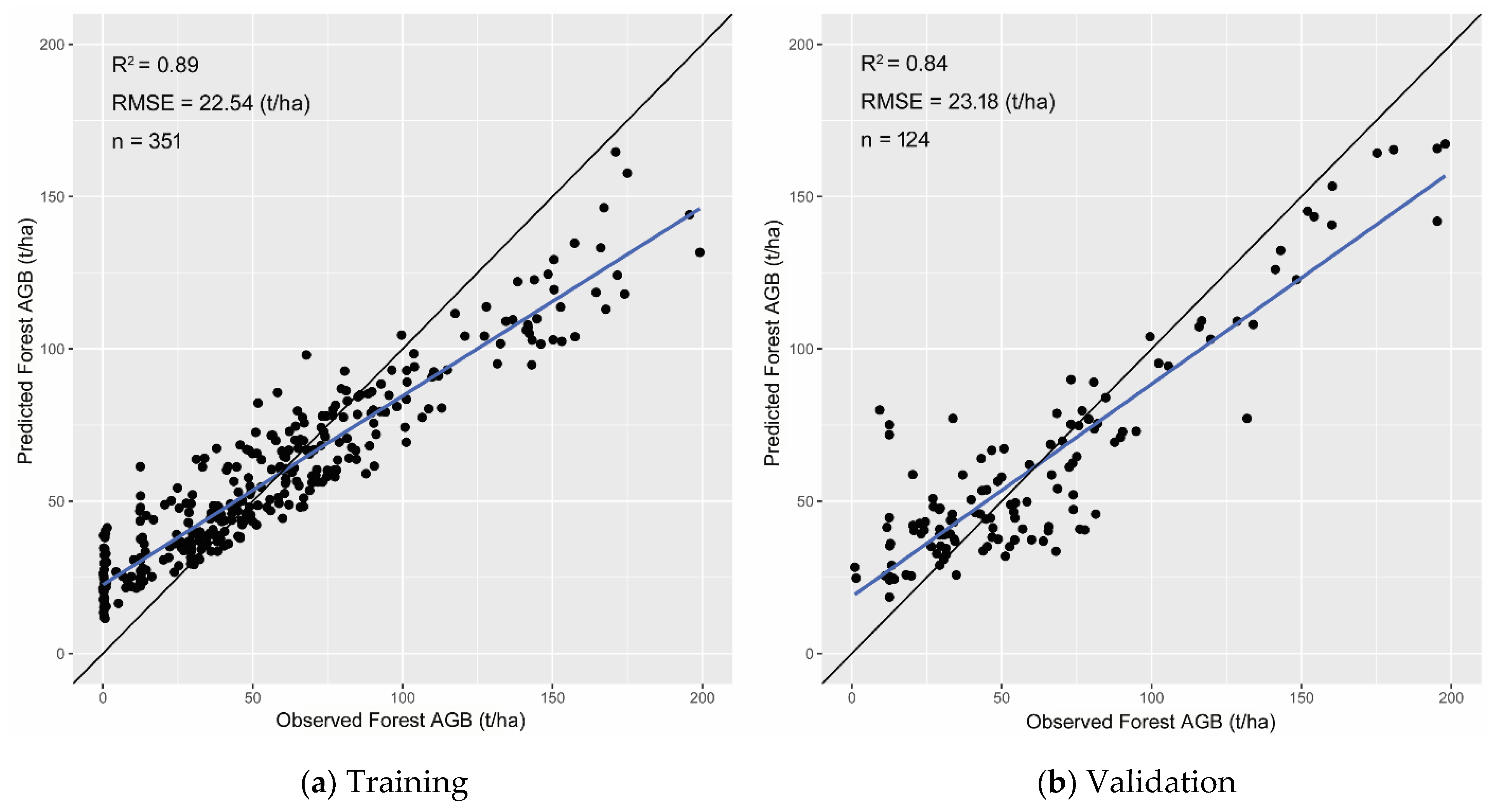
3.2. RF Approach Outperforms KNN and MLR Approach

RF performed better than KNN and MLR in estimating forest AGB using both MOD09A1 and FY-3C VIRR imagery (Table 4). All the models were significant at a p-value < 0.001. The same set of referenced data of forest AGB from the NFRI dataset was input into the models, making it possible to compare the performances of the two satellite image products in estimating forest AGB and to help understand factors that influence accuracies. The performance ranking of the three models was the same for MOD09A1 and FY-3C VIRR imagery.
As a result, five variables from MOD09A1 were selected to create an MLR model after a stepwise regression, with R2 of 0.32:
AGBMOD09A1 = 52.394 + 97.979 ∗ NDIIb6 − 242.903 ∗ VARI + 8.613 ∗ RVI + 191.119 ∗ ARVI + 230.540 ∗ NDWI.
In contrast, the MLR model based on variables from FY-3C VIRR has a slightly lower R2 of 0.29. Three variables were involved after a stepwise regression:
AGBFY-3C = −28.01 + 80.95 ∗ NDIIb6 + 312.29 ∗ Green + 58.81 ∗ ARVI.
After testing, the optimal KNN model based on MOD09A1 variables was established with the parameter K = 9 and an R2 value of 0.65, and the best K value of the KNN model for FY-3C variables was 7, with an R2 value of 0.58. The RF models for MOD09A1 and FY-3C VIRR imageries achieved R2 values of 0.84 and 0.81, respectively, and RMSE of 23.18 and 23.43, respectively (Table 4).
The MLR models performed worst on both satellite imageries when compared to the KNN and RF models, as indicated by the comparatively lower R2 values. This suggests that the models have low degrees of fitting to the observed values, probably due to a weak linear or nonlinear relationship between forest AGB and the remote sensing variables. All of the predictor variables from MOD09A1 and FY-3C VIRR have VIF values larger than 10. This indicates that the variables used for MLR models have serious multicollinearity, which also leads to poor performance of MLR modeling. RF modeling performed better for both imageries than the other two approaches. It showed a strong ability to avoid overfitting.
It is noticeable that variables from MOD09A1 performed marginally better than using those from FY-3C VIRR in RF models on both the training dataset and validation dataset (Figure 4 and Figure 5). This indicates that forest AGB could achieve comparable accuracy using either MOD09A1 or FY-3C VIRR images. For both kinds of imagery, RF models predicted lower forest AGB with higher accuracy compared to predicting higher forest AGB with lower accuracy (Figure 4 and Figure 5), which may be due to the saturation of spectral signals at higher biomass values. Further comparison was conducted to reveal the difference between the two estimations of forest AGB from MOD09A1 and FY-3C VIRR imageries, respectively, by RF models. Moreover, in this study, the RF model with the input of MOD09A1 imagery was selected for forest AGB mapping and to help understand the spatial distribution pattern of forest AGB in Yunnan Province.

3.3. Comparison of Forest AGB Estimation by RF Models Based on the Two Imageries

The total amounts of forest AGB estimated using MOD09A1 and FY-3C VIRR imageries by RF methods were greater than that of the NFRI dataset (Figure 6), by 4.13% and 6.25%, respectively. The total mean of forest AGB from FY-3C imagery (62.10 t/ha) was higher than the means from the NFRI dataset and MOD09A1 imagery (58.91 t/ha and 58.05 t/ha, respectively). This is probably attributable to the larger estimation in both the mean value of forest AGB (47.77 t/ha) and the proportion of the largest share of forest AGB range (30–60 t/ha) by FY-3C VIRR imagery. The mean AGB, at the 0–30 t/ha range, obtained from MOD09A1 and FY-3C VIRR was similar (24.52 t/ha and 23.77 t/ha, respectively) and was the same for the ranges of 30–60 t/ha and 60–90 t/ha (47.80 t/ha and 47.77 t/ha, 84.25 t/ha and 84.58 t/ha, respectively). The total amounts of forest AGB at the two ranges below 60 t/ha from the two imageries were almost identical. The mean values of forest AGB estimated using the two imageries were higher than that of the NRFI dataset at the three ranges lower than 90 t/ha. The underestimation in forest AGB modeled by remote sensing data at the AGB ranges higher than 90 t/ha was due to signal saturation in optical remote sensing data at high forest AGB. Higher forest AGB was associated with a greater discrepancy between estimations derived from remote sensing data and observation values.

3.4. Mapping of Forest AGB Distribution by Forest Zones and Dominant Tree Species

Figure 7 shows that the forest AGB distribution in Yunnan mapped by MOD09A1 and FY-3C VIRR imageries is similar. AGB was found to be high mainly at the northwestern, western, southwestern and southern periphery of the province, in contrast to low AGB, which was mainly located in the central and eastern parts of the province. The color scheme of Figure 7 shows that the prediction of forest AGB by FY-3C VIRR imagery had larger variation. Because the RF algorithm based on MOD09A1 images has achieved the highest accuracy in forest AGB mapping, we employed this combination to estimate forest AGB. Then, we produced a map of its spatial distribution in Yunnan Province and used it for further statistical analysis to show the spatial distribution pattern of forest AGB.
The total forest AGB in Yunnan Province is 2123.22 Mt, with a mean value of 58.05 t/ha. The cold-temperate coniferous forest zone in the northwest has the highest mean forest AGB density, 76.08 t/ha, followed by the tropical broadleaved forest zone at 75.40 t/ha. These two forest zones contribute 8.39% and 18.08% of the total forest AGB of Yunnan Province, respectively. The lowest mean forest AGB density (43.52 t/ha) occurs in the warm evergreen broadleaved forest zone. The warm evergreen broadleaved and coniferous forest zone has a relatively low AGB density (49.45 t/ha), which accounts for the largest proportion (39.93%) of the total forest AGB in the study area due to the large area that it covers. The distribution pattern of high forest AGB is consistent with the spatial distribution of the key areas of forest conservation and biodiversity conservation in recent decades, e.g., national and provincial protected areas and ecological forest protection.
Abies fabri, mainly located in northwest Yunnan, had the highest AGB density among all the dominant tree species at 115.93 t/ha, followed by Quercus spp. at 88.52 t/ha, other broadleaved species (a group of broadleaved tree species except for Quercus spp., Alnus cremastogyne and Betula spp.) forest at 85.61 t/ha and Pinus kesiya var. langbianensis at 81.23 t/ha. Pinus densata, Pinus yunnanensis and Pinus armandii had relatively low AGB density, with values of 61.35 t/ha, 55.42 t/ha and 51.63 t/ha, respectively. Quercus spp., Pinus yunnanensis, other broadleaved forests and Pinus kesiya var. langbianensis were the top four important forests, accounting for 14.50%, 13.20%, 12.35% and 5.83% of the total forest AGB in Yunnan Province.

4. Discussion

In this study, we mapped the forest AGB in Yunnan Province, an important region for carbon storage, using three approaches with MODIS and FY-3C imageries. The results indicate that RF performed best out of all the approaches for forest AGB modeling. The thematic map by MOD09A1 images achieved marginally better accuracy than the map by FY-3C VIRR images. Although MODIS imagery has been used for national forest AGB mapping in China and other regions, this study was the first to adopt FY series imagery for this purpose and to conduct a comparison of these two imageries. Our results indicate that FY-3C VIRR imagery achieved acceptable accuracy, relative to MOD09A1 imagery, in mapping forest AGB at the regional scale.

4.1. Contribution of Spectral Index Variables

We found that although MOD09A1 and FY-3C VIRR imageries have different spatial resolutions, some common features can be detected in the predictor variables. Among the predictor variables derived, NDIIb6 outperformed all the other variables for both imageries, respectively, and both ARVI and VARI also ranked in the top 10 of important variables. This could be one of the reasons for the consistency of predictions of forest AGB between MOD09A1 and FY-3C VIRR imageries (R2 > 0.80).
Indices of vegetation water content often correlate with vegetation health and vigor and indicate vegetation biomass [65]. Our study demonstrated a close relationship between these indices and forest AGB. NDIIb6 and NDIIb7 derived from near-infrared (NIR) and SWIR centering at 1640 nm and 2130 nm bands, respectively, showed great potential for vegetation water content estimation in previous studies [65,66], as the water content in vegetation was very important for photosynthesis leading to biomass formation. These NDII indices were named the normalized difference water index (NDWI), NDIIb6 as NDWI1640 and NDIIb7 as NDWI2130. The fact that NDII was less sensitive to the bandwidth of different sensors, as proven by Chen et al. [67], was also confirmed by this study. The vegetation–water content-related index NDMI based on NIR (860 nm) and SWIR (1240 nm) is also one of the top 10 important predictor variables from MOD09A1 imagery. Gao (1996) demonstrated the sensitivity of this index to changes in the water content of vegetation canopies and showed that it is less sensitive to atmospheric effects than NDVI [44]. A positive correlation between vegetation water content and vegetation biomass was also revealed by Xing et al. [68] and Momen et al. [69]. ARVI and VARI are the two common and important indices related to vegetation greenness from MOD09A1 and FY-3C VIRR imageries, both enhanced by the presence of the blue channel to minimize the atmospheric effects.

4.2. The Ability of MOD09A1 and FY-3C VIRR to Map Forest AGB

The ability of remote sensing data to map forest AGB depends on the sensitivity of the predictor variables selected for mapping forest AGB and on the complexity of the vegetation structure. Our results showed acceptable accuracies of forest AGB estimation by both imageries, although the performance of MOD09A1 was marginally better than that of FY-3C VIRR by RF modeling. This indicates that the suitability of the two imageries for forest AGB prediction is comparable. The comparable applicability of MOD09A1 and FY-3C VIRR imageries for forest AGB at the regional scale can be attributable to their similarity in spectral architectures, temporal resolution and geographical coverage. MOD09A1 and FY-3C VIRR have spectral compositions for visible light and near-infrared, as well as for the overlapped range of infrared, which makes it possible to calculate vegetation indices for modeling. Both imageries have short revisit cycles of 1–2 days and large geographical coverage extents of over 2000 km2. These features enable efficient image processing for monitoring the dynamics of forest AGB at regional and global scales.
The difference in the performance of AGB estimation can be attributed to the difference in the spectrum ranges and spatial resolution of the two imageries. The spectrum range of MOD09A1 used for calculating variables to model forest AGB is slightly wider than that of FY-3C VIRR, particularly in SWIR. MOD09A1 has two indices related to vegetation water content (NDIIb7 and NDMI), more than FY-3C VIRR. These two indices are absent for FY-3C due to the lack of two specific SWIR bands for index calculation. Thus, to some extent, MOD09A1 provides more spectral information in forest AGB estimation.
The higher spatial resolution of MOD09A1 (500 m) could account for the higher accuracy of forest AGB mapping compared to FY-3C VIRR (1000 m). This finding is consistent with previous findings of forest AGB mapping by finer resolution satellite imagery with higher accuracy [70,71]. Because the average area of forest stand polygons in the NFRI dataset of Yunnan Province is approximately 9 hectares, which is smaller than single pixels of MOD09A1 and FY-3C VIRR imageries, the spectral information from individual bands and vegetation indices used for modeling was “aggregated” and “averaged”. Higher spatial resolutions are expected to achieve higher accuracies [71].

4.3. Performance of Parametric and Nonparametric Approaches

In our study, the adopted parametric approach, the MLR model, was found to have performed poorly in forest AGB prediction, which was also confirmed by other studies [5]. Linear regression is used for modeling when remote sensing variables have a strong linear relationship with biomass and a weak relationship with selected remote sensing variables themselves. However, biomass is often nonlinearly related to remote sensing variables [24,54]; thus, MLR models may lead to low accuracy in predictions.
Our results found that nonparametric approaches achieved higher accuracy compared to the parametric approach in mapping forest AGB, which is consistent with previous studies [7,24,56,72]. Lu et al. (2016) suggested that nonparametric approaches should be explored if large representative field datasets exist for calibration [24]. In our study, we selected forest AGB reference data by stratified forest-type zones as an effective way to ensure the representativeness of reference datasets.

5. Conclusions

In this study, we compared forest AGB estimation for Yunnan Province, southwest of China, with MOD09A1 and FY-3C VIRR imagery by applying one parametric approach, MLR, and two nonparametric approaches, KNN and RF. Reference data of forest AGB from the NFRI dataset, individual spectral bands and the derived vegetation indices were used to establish the models. The results indicated that (1) RF models outperformed the MLR and KNN models for both imageries using the same sampled forest AGB reference dataset from NFRI data. (2) Among all the remote sensing variables, NDIIb6 related to the moisture of vegetation canopy was the most sensitive to forest AGB for both imageries. Vegetation greenness indices contributed more to AGB prediction based on MOD09A1 than those based on FY-3C VIRR, while individual spectral bands of FY-3C played a more important role than vegetation greenness indices. (3) FY-3C VIRR imagery had high potential to be an alternative data source substituting the MODIS data for forest AGB mapping at regional scales.
This study examined overall forest AGB estimation using MODIS and FY imageries. However, spectral saturation at high forest AGB is a challenge for AGB mapping with optical satellite imagery; further studies involving the sensitivity of spectral variables of these imageries to forest AGB need to be conducted, and as FY imagery is a new option as a data source for AGB mapping, solutions need to be explored for improving mapping accuracy. Moreover, the real-time forest AGB monitoring or quantifying AGB change at regional scales could be an applicative aspect for FY series satellite imagery.

Author Contributions

H.C. and Z.Q. designed the study; H.C. conducted the data analysis, modeling forest AGB and wrote the draft of the manuscript; H.C., Z.Q. and D.-L.Z. improved the manuscript; G.O. obtained NFRI dataset and provided support to the study; X.L. and G.Z. conducted statistical analysis; J.F. and C.Z. collected and preprocessed the FY-3C VIRR data. H.X. supervised and coordinated the research project. All authors have read and agreed to the published version of the manuscript.

Funding

This study was financially supported by the National Natural Science Foundation of China (grant number 31770677).

Data Availability Statement

Data from this study will be available upon request to the authors.

Acknowledgments

We sincerely thank Dietrich Schmidt-Vogt for checking the English grammar of the manuscript.

Conflicts of Interest

The authors declare no conflict of interest.

Appendix A

Figure A1. The true-color MOD09A1 (a) and FY-3C VIRR (b) imageries of Yunnan Province, with the dots showing the sampling points to estimate forest AGB.
Remotesensing 14 05456 g0a1

References

  1. Yin, G.; Zhang, Y.; Sun, Y.; Wang, T.; Zeng, Z.; Piao, S. MODIS Based Estimation of Forest Aboveground Biomass in China. PLoS ONE 2015, 10, e0130143. [Google Scholar] [CrossRef] [PubMed] [Green Version]
  2. Goodale, C.L.; Apps, M.J.; Birdsey, R.A.; Field, C.B.; Heath, L.S.; Houghton, R.A.; Jenkins, J.C.; Kohlmaier, G.H.; Kurz, W.; Liu, S.R.; et al. Forest carbon sinks in the Northern Hemisphere. Ecol. Appl. 2002, 12, 891–899. [Google Scholar] [CrossRef]
  3. Houghton, R.A. Aboveground forest biomass and the global carbon balance. Glob. Chang. Biol. 2005, 11, 945–958. [Google Scholar] [CrossRef]
  4. Pan, Y.D.; Birdsey, R.A.; Fang, J.Y.; Houghton, R.; Kauppi, P.E.; Kurz, W.A.; Phillips, O.L.; Shvidenko, A.; Lewis, S.L.; Canadell, J.G.; et al. A Large and Persistent Carbon Sink in the World′s Forests. Science 2011, 333, 988–993. [Google Scholar] [CrossRef] [PubMed] [Green Version]
  5. Ou, G.L.; Lv, Y.Y.; Xu, H.; Wang, G.X. Improving Forest Aboveground Biomass Estimation of Pinus densata Forest in Yunnan of Southwest China by Spatial Regression using Landsat 8 Images. Remote Sens. 2019, 11, 2750. [Google Scholar] [CrossRef] [Green Version]
  6. Chi, H.; Sun, G.Q.; Huang, J.L.; Guo, Z.F.; Ni, W.J.; Fu, A.M. National Forest Aboveground Biomass Mapping from ICESat/GLAS Data and MODIS Imagery in China. Remote Sens. 2015, 7, 5534–5564. [Google Scholar] [CrossRef] [Green Version]
  7. Lu, D.S. The potential and challenge of remote sensing-based biomass estimation. Int. J. Remote Sens. 2006, 27, 1297–1328. [Google Scholar] [CrossRef]
  8. Dong, J.R.; Kaufmann, R.K.; Myneni, R.B.; Tucker, C.J.; Kauppi, P.E.; Liski, J.; Buermann, W.; Alexeyev, V.; Hughes, M.K. Remote sensing estimates of boreal and temperate forest woody biomass: Carbon pools, sources, and sinks. Remote Sens. Environ. 2003, 84, 393–410. [Google Scholar] [CrossRef] [Green Version]
  9. Calvao, T.; Palmeirim, J.M. Mapping Mediterranean scrub with satellite imagery: Biomass estimation and spectral behaviour. Int. J. Remote Sens. 2004, 25, 3113–3126. [Google Scholar] [CrossRef]
  10. Zhang, Y.; Liang, S.; Yang, L. A Review of Regional and Global Gridded Forest Biomass Datasets. Remote Sens. 2019, 11, 2744. [Google Scholar] [CrossRef]
  11. Li, X.; Zhang, M.; Long, J.; Lin, H. A Novel Method for Estimating Spatial Distribution of Forest Above-Ground Biomass Based on Multispectral Fusion Data and Ensemble Learning Algorithm. Remote Sens. 2021, 13, 3910. [Google Scholar] [CrossRef]
  12. Cooper, S.; Okujeni, A.; Pflugmacher, D.; van der Linden, S.; Hostert, P. Combining simulated hyperspectral EnMAP and Landsat time series for forest aboveground biomass mapping. Int. J. Appl. Earth Obs. Geoinf. 2021, 98, 102307. [Google Scholar] [CrossRef]
  13. Kumar, L.; Mutanga, O. Remote Sensing of Above-Ground Biomass. Remote Sens. 2017, 9, 935. [Google Scholar] [CrossRef] [Green Version]
  14. Foody, G.M.; Boyd, D.S.; Cutler, M.E.J. Predictive relations of tropical forest biomass from Landsat TM data and their transferability between regions. Remote Sens. Environ. 2003, 85, 463–474. [Google Scholar] [CrossRef]
  15. Steininger, M.K. Satellite estimation of tropical secondary forest above-ground biomass: Data from Brazil and Bolivia. Int. J. Remote Sens. 2000, 21, 1139–1157. [Google Scholar] [CrossRef]
  16. Baccini, A.; Friedl, M.A.; Woodcock, C.E.; Warbington, R. Forest biomass estimation over regional scales using multisource data. Geophys. Res. Lett. 2004, 31, L10501. [Google Scholar] [CrossRef] [Green Version]
  17. Lu, D. Aboveground biomass estimation using Landsat TM data in the Brazilian Amazon. Int. J. Remote Sens. 2005, 26, 2509–2525. [Google Scholar] [CrossRef]
  18. Rahman, M.M.; Csaplovics, E.; Koch, B. An efficient regression strategy for extracting forest biomass information from satellite sensor data. Int. J. Remote Sens. 2005, 26, 1511–1519. [Google Scholar] [CrossRef]
  19. Zhou, J.J.; Zhao, Z.; Zhao, Q.X.; Zhao, J.; Wang, H.Z. Quantification of aboveground forest biomass using Quickbird imagery, topographic variables, and field data. J. Appl. Remote Sens. 2013, 7, 073484. [Google Scholar] [CrossRef]
  20. Gomez, J.A.; Zarco-Tejada, P.J.; Garcia-Morillo, J.; Gama, J.; Soriano, M.A. Determining Biophysical Parameters for Olive Trees Using CASI-Airborne and Quickbird-Satellite Imagery. Agron. J. 2011, 103, 644–654. [Google Scholar] [CrossRef]
  21. Gomez, C.; Wulder, M.A.; Montes, F.; Delgado, J.A. Modeling Forest Structural Parameters in the Mediterranean Pines of Central Spain using QuickBird-2 Imagery and Classification and Regression Tree Analysis (CART). Remote Sens. 2012, 4, 135–159. [Google Scholar] [CrossRef] [Green Version]
  22. Zhu, Y.H.; Liu, K.; Liu, L.; Wang, S.G.; Liu, H.X. Retrieval of Mangrove Aboveground Biomass at the Individual Species Level with WorldView-2 Images. Remote Sens. 2015, 7, 12192–12214. [Google Scholar] [CrossRef] [Green Version]
  23. Qiu, P.H.; Wang, D.Z.; Zou, X.Q.; Yang, X.; Xie, G.Z.; Xu, S.J.; Zhong, Z.Q. Finer Resolution Estimation and Mapping of Mangrove Biomass Using UAV LiDAR and WorldView-2 Data. Forests 2019, 10, 871. [Google Scholar] [CrossRef] [Green Version]
  24. Lu, D.S.; Chen, Q.; Wang, G.X.; Liu, L.J.; Li, G.Y.; Moran, E. A survey of remote sensing-based aboveground biomass estimation methods in forest ecosystems. Int. J. Digit. Earth 2016, 9, 63–105. [Google Scholar] [CrossRef]
  25. Zhang, J.L.; Lu, C.; Xu, H.; Wang, G.X. Estimating aboveground biomass of Pinus densata-dominated forests using Landsat time series and permanent sample plot data. J. For. Res. 2019, 30, 1689–1706. [Google Scholar] [CrossRef]
  26. Fassnacht, F.E.; Hartig, F.; Latifi, H.; Berger, C.; Hernandez, J.; Corvalan, P.; Koch, B. Importance of sample size, data type and prediction method for remote sensing-based estimations of aboveground forest biomass. Remote Sens. Environ. 2014, 154, 102–114. [Google Scholar] [CrossRef]
  27. Zhang, Q.L.; He, H.S.; Liang, Y.; Hawbaker, T.J.; Henne, P.D.; Liu, J.X.; Huang, S.L.; Wu, Z.W.; Huang, C. Integrating forest inventory data and MODIS data to map species-level biomass in Chinese boreal forests. Can. J. For. Res. 2018, 48, 461–479. [Google Scholar] [CrossRef]
  28. Lu, J.; Feng, Z.; Zhu, Y. Estimation of Forest Biomass and Carbon Storage in China Based on Forest Resources Inventory Data. Forests 2019, 10, 650. [Google Scholar] [CrossRef] [Green Version]
  29. Forestry Department of Yunnan Province. Report of Forest Resource Survey in Yunnan Province; Yunnan Science and Technology Press: Kunming, China, 2017. [Google Scholar]
  30. Forestry Department of Yunnan Province. Forest Resources in Yunnan; Yunnan Science and Technology Press: Kunming, China, 2018. [Google Scholar]
  31. Chen, F.; Niu, S.; Tong, X.; Zhao, J.; Sun, Y.; He, T. The Impact of Precipitation Regimes on Forest Fires in Yunnan Province, Southwest China. Sci. World J. 2014, 326782. [Google Scholar] [CrossRef] [Green Version]
  32. Editting Committee of Yunnan Forest. Yunnan Forest; China Forestry Press: Beijing, China; Yunnan Science and Technology Press: Kunming, China, 1986. [Google Scholar]
  33. Weng, E.S.; Zhou, G.S. Modeling distribution changes of vegetation in China under future climate change. Env. Model Assess 2006, 11, 45–58. [Google Scholar] [CrossRef]
  34. Yongqian, W.; Dejun, Z.; Liang, S.; Shiqi, Y.; Tang, S.; Yanghua, G.; Qinyu, Y.; Hao, Z. Evaluating FY3C-VIRR reconstructed land surface temperature in cloudy regions. Eur. J. Remote Sens. 2021, 54, 266–280. [Google Scholar] [CrossRef]
  35. Guo, N.; Wang, X.; Cai, D.; Yang, J. Comparison and evaluation between MODIS vegetation indices in Northwest China. In Proceedings of the IEEE International Geoscience and Remote Sensing Symposium (IGARSS), Barcelona, Spain, 23–27 July 2007; p. 3366. [Google Scholar]
  36. Rouse, J.W.; Haas, R.H.; Schell, J.A.; Deering, D.W. Monitoring vegetation systems in the Great Plains with ERTS. NASA Spe. 1974, 351, 309–317. [Google Scholar]
  37. Huete, A.; Didan, K.; Miura, T.; Rodriguez, E.P.; Gao, X.; Ferreira, L.G. Overview of the radiometric and biophysical performance of the MODIS vegetation indices. Remote Sens. Environ. 2002, 83, 195–213. [Google Scholar] [CrossRef]
  38. Jordan, C.F. Derivation of leaf-area index from quality of light on forest floor. Ecology 1969, 50, 663. [Google Scholar] [CrossRef]
  39. Kaufman, Y.J.; Tanre, D. Atmospherically resistant vegetation index (ARVI) for EOS-MODIS. IEEE Trans. Geosci. Remote Sens. 1992, 30, 261–270. [Google Scholar] [CrossRef]
  40. Huete, A.R. A soil-adjusted vegetation index (SAVI). Remote Sens. Environ. 1988, 25, 295–309. [Google Scholar] [CrossRef]
  41. Qi, J.; Chehbouni, A.; Huete, A.R.; Kerr, Y.H.; Sorooshian, S. A modified soil adjusted vegetatiob index. Remote Sens. Environ. 1994, 48, 119–126. [Google Scholar] [CrossRef]
  42. Gitelson, A.A.; Kaufman, Y.J.; Stark, R.; Rundquist, D. Novel algorithms for remote estimation of vegetation fraction. Remote Sens. Environ. 2002, 80, 76–87. [Google Scholar] [CrossRef] [Green Version]
  43. Hunt, E.R.; Rock, B.N. Detection of Changes in Leaf Water-Content Using near-Infrared and Middle-Infrared Reflectances. Remote Sens. Environ. 1989, 30, 43–54. [Google Scholar]
  44. Gao, B.C. NDWI—A normalized difference water index for remote sensing of vegetation liquid water from space. Remote Sens. Environ. 1996, 58, 257–266. [Google Scholar] [CrossRef]
  45. Wilson, E.H.; Sader, S.A. Detection of forest harvest type using multiple dates of Landsat TM imagery. Remote Sens. Environ. 2002, 80, 385–396. [Google Scholar] [CrossRef]
  46. McFeeters, S.K. The use of the normalized difference water index (NDWI) in the delineation of open water features. Int. J. Remote Sens. 1996, 17, 1425–1432. [Google Scholar] [CrossRef]
  47. Bi, Y.; Yang, Z.; Zhang, P.; Sun, Y.; Bai, W.; Du, Q.; Yang, G.; Chen, J.; Liao, M. An introduction to China FY3 radio occultation mission and its measurement simulation. Adv. Sp. Res. 2012, 49, 1191–1197. [Google Scholar] [CrossRef]
  48. Dong, P.M.; Huang, J.P.; Liu, G.Q.; Zhang, T. Assimilation of FY-3A microwave observations and simulation of brightness temperature under cloudy and rainy condition. J. Trop. Meteorol. 2014, 30, 302–310. [Google Scholar]
  49. Yang, Y.M.; Du, M.B.; Zhang, J. Experiments of assimilating FY-3A microwave data in forecast of typhoon Morakot. J. Trop. Meteorol. 2012, 28, 23–30. [Google Scholar]
  50. Wang, W.; Zhang, X.; An, X.; Zhang, Y.; Huang, F.; Wang, Y.; Wang, Y.; Zhang, Z.; Lue, J.; Fu, L.; et al. Analysis for retrieval and validation results of FY-3 Total Ozone Unit (TOU). China Sci. Bull. 2010, 55, 3037–3043. [Google Scholar] [CrossRef]
  51. Fang, J.Y.; Wang, G.G.; Liu, G.H.; Xu, S.L. Forest biomass of China: An estimate based on the biomass-volume relationship. Ecol. Appl. 1998, 8, 1084–1091. [Google Scholar]
  52. Mitchard, E.T.A.; Saatchi, S.S.; Lewis, S.L.; Feldpausch, T.R.; Woodhouse, I.H.; Sonke, B.; Rowland, C.; Meir, P. Measuring biomass changes due to woody encroachment and deforestation/degradation in a forest-savanna boundary region of central Africa using multi-temporal L-band radar backscatter. Remote Sens. Environ. 2011, 115, 2861–2873. [Google Scholar] [CrossRef] [Green Version]
  53. Sun, G.; Ranson, K.J.; Guo, Z.; Zhang, Z.; Montesano, P.; Kimes, D. Forest biomass mapping from lidar and radar synergies. Remote Sens. Environ. 2011, 115, 2906–2916. [Google Scholar] [CrossRef] [Green Version]
  54. Lu, D.; Chen, Q.; Wang, G.; Moran, E.; Batistella, M.; Zhang, M.; Laurin, G.V.; Saah, D. Aboveground Forest Biomass Estimation with Landsat and LiDAR Data and Uncertainty Analysis of the Estimates. Int. J. For. Res. 2012, 2012, 436537. [Google Scholar] [CrossRef] [Green Version]
  55. Zhao, P.; Lu, D.; Wang, G.; Liu, L.; Li, D.; Zhu, J.; Yu, S. Forest aboveground biomass estimation in Zhejiang Province using the integration of Landsat TM and ALOS PALSAR data. Int. J. Appl. Earth Obs. Geoinf. 2016, 53, 1–15. [Google Scholar] [CrossRef]
  56. Lee, H.; Wang, J.; Leblon, B. Using Linear Regression, Random Forests, and Support Vector Machine with Unmanned Aerial Vehicle Multispectral Images to Predict Canopy Nitrogen Weight in Corn. Remote Sens. 2020, 12, 2071. [Google Scholar] [CrossRef]
  57. Breiman, L. Random Forests. Mach. Learn. 2001, 45, 5–32. [Google Scholar] [CrossRef] [Green Version]
  58. Ahmad, A.; Gilani, H.; Ahmad, S.R. Forest Aboveground Biomass Estimation and Mapping through High-Resolution Optical Satellite Imagery-A Literature Review. Forests 2021, 12, 914. [Google Scholar] [CrossRef]
  59. Li, Z.; Bi, S.; Hao, S.; Cui, Y. Aboveground biomass estimation in forests with random forest and Monte Carlo-based uncertainty analysis. Ecol. Indic. 2022, 142, 109246. [Google Scholar] [CrossRef]
  60. Li, Y.; Li, M.; Li, C.; Liu, Z. Forest aboveground biomass estimation using Landsat 8 and Sentinel-1A data with machine learning algorithms. Sci. Rep. 2020, 10, 9952. [Google Scholar] [CrossRef]
  61. Esteban, J.; McRoberts, R.E.; Fernandez-Landa, A.; Luis Tome, J.; Naesset, E. Estimating Forest Volume and Biomass and Their Changes Using Random Forests and Remotely Sensed Data. Remote Sens. 2019, 11, 1944. [Google Scholar] [CrossRef] [Green Version]
  62. Zeng, N.; Ren, X.; He, H.; Zhang, L.; Zhao, D.; Ge, R.; Li, P.; Niu, Z. Estimating grassland aboveground biomass on the Tibetan Plateau using a random forest algorithm. Ecol. Indic. 2019, 102, 479–487. [Google Scholar] [CrossRef]
  63. Yang, H.; Li, F.; Wang, W.; Yu, K. Estimating Above-Ground Biomass of Potato Using Random Forest and Optimized Hyperspectral Indices. Remote Sens. 2021, 13, 2339. [Google Scholar] [CrossRef]
  64. McRoberts, R.E.; Naesset, E.; Gobakken, T. Optimizing the k-Nearest Neighbors technique for estimating forest aboveground biomass using airborne laser scanning data. Remote Sens. Environ. 2015, 163, 13–22. [Google Scholar] [CrossRef]
  65. Zhang, F.; Zhou, G. Estimation of vegetation water content using hyperspectral vegetation indices: A comparison of crop water indicators in response to water stress treatments for summer maize. BMC Ecol. 2019, 19, 18. [Google Scholar] [CrossRef] [PubMed] [Green Version]
  66. Yi, Y.; Yang, D.; Chen, D.; Huang, J. Retrieving crop physiological parameters and assessing water deficiency using MODIS data during the winter wheat growing period. Can. J. Remote Sens. 2007, 33, 189–202. [Google Scholar] [CrossRef] [Green Version]
  67. Chen, X.; Wang, S.; Zhang, L.; Jiang, H. Accuracy and Sensitivity of Retrieving Vegetation Leaf Water Content. Remote Sens. Inf. 2016, 31, 48–57. [Google Scholar]
  68. Xing, M.; He, B.; Li, X. Integration method to estimate above-ground biomass in arid prairie regions using active and passive remote sensing data. J. Appl. Remote Sens. 2014, 8, 083677. [Google Scholar] [CrossRef]
  69. Momen, M.; Wood, J.D.; Novick, K.A.; Pangle, R.; Pockman, W.T.; McDowell, N.G.; Konings, A.G. Interacting Effects of Leaf Water Potential and Biomass on Vegetation Optical Depth. J. Geophys. Res. Biogeo. 2017, 122, 3031–3046. [Google Scholar] [CrossRef]
  70. Salajanu, D.; Jacobs, D.M. Accuracy assessment of biomass and forested area classification from modis, landstat-tm satellite imagery and forest inventory plot data. In Proceedings of the ASPRS 2007 Annual Conference, Tampa, FL, USA, 7–11 May 2007. [Google Scholar]
  71. Jha, N.; Tripathi, N.K.; Barbier, N.; Virdis, S.G.P.; Chanthorn, W.; Viennois, G.; Brockelman, W.Y.; Nathalang, A.; Tongsima, S.; Sasaki, N.; et al. The real potential of current passive satellite data to map aboveground biomass in tropical forests. Remote Sens. Ecol. Conserv. 2021, 7, 504–520. [Google Scholar] [CrossRef]
  72. Tian, X.; Su, Z.; Chen, E.; Li, Z.; van der Tol, C.; Guo, J.; He, Q. Estimation of forest above-ground biomass using multi-parameter remote sensing data over a cold and arid area. Int. J. Appl. Earth Obs. Geoinf. 2012, 14, 160–168. [Google Scholar]
Figure 1. The location of Yunnan Province in China, topography and forest type zones: ① cold-temperate coniferous forest, ② warm evergreen broadleaved forest, ③ warm evergreen broadleaved and coniferous forest, ④ warm–hot broadleaved and coniferous forest and ⑤ tropical broadleaved forest.
Remotesensing 14 05456 g001
Figure 2. The flowchart of methodology.
Remotesensing 14 05456 g002
Figure 3. The variable importance plots for MOD09A1 images (a) and FY-3C VIRR Images (b).
Remotesensing 14 05456 g003
Figure 4. Observed versus predicted forest AGB applying random forest (RF) model and MOD09A1 imagery for (a) the training dataset and (b) the validation dataset.
Remotesensing 14 05456 g004
Figure 5. Observed versus predicted forest AGB applying random forest (RF) model and FY-3C VIRR imagery for (a) the training dataset and (b) the validation dataset.
Remotesensing 14 05456 g005
Figure 6. Distribution of forest AGB in the Chinese National Forest Resource Inventory (NFRI) dataset and estimated forest AGB based on MOD09A1 and FY-3C VIRR imageries by RF models.
Remotesensing 14 05456 g006
Figure 7. Forest AGB maps derived from (a) MOD09A1 and (b) FY-3C imageries based on RF models. Forest type zones: ① cold-temperate coniferous forest, ② warm evergreen broadleaved forest, ③ warm evergreen broadleaved and coniferous forest, ④ warm–hot broadleaved and coniferous forest and ⑤ tropical broadleaved forest.
Remotesensing 14 05456 g007
Table 1. The spectral characteristics of MOD09A1 bands.
Band#NameSpectral Range (nm)Center Wavelength (nm)Bandwidth (nm)
1Red620–67064550
2Near Infrared (NIR)841–87685935
3Blue459–47946920
4Green545–56555520
5Shortwave infrared (SWIR1240)1230–1250124020
6Shortwave infrared (SWIR1640)1628–1652164024
7Shortwave infrared (SWIR2130)2105–2155213050
Table 2. The vegetation indices derived from MOD09A1 and FY-3C VIRR imagery.
IndexFormulaMOD09A1FY-3C VIRRReference
Vegetation greenness indicesNDVI(NIR − RED)/(NIR + RED)Rouse et al. [36]
EVI2.5(NIR − RED)/[(NIR + 6RED − 7.5BLUE) + 1]Huete et al. [37]
RVINIR/REDJordan [38]
ARVI[NIR − (2 RED − BLUE)]/[NIR) + (2RED − BLUE)]Kaufman and Tanre [39]
SAVI(1 + 0.5)(NIR − RED)/(NIR + RED + 0.5)Huete [40]
MSAVI[2NIR + 1 − ( 2 NIR + 1 ) 2 − 8(NIR − RED)]/2Qi et al. [41]
VARI(GREEN − RED)/(GREEN + RED − BLUE)Gitelson et al. [42]
Vegetation water indicesNDIIb6(NIR − SWIR1640)/(NIR + SWIR1640)√ *Hunt and Rock [43]
NDIIb7(NIR − SWIR2130)/(NIR + SWIR2130)NAHunt and Rock [43]
NDMI(NIR − SWIR1240)/(NIR + SWIR1240)NAGao [44], Wilson [45]
NDWI(GREEN − NIR)/(GREEN + NIR)Mcfeeters [46]
NDVI = normalized difference of vegetation index; EVI = enhanced vegetation index; RVI = ratio vegetation index; ARVI = atmospherically resistant vegetation index; SAVI = soil adjusted vegetation index; MSAVI = modified soil adjusted vegetation index; VARI = visible atmospherically resistant index; NDIIb6 = normalized difference of infrared index—band6; NDIIb7 = normalized difference of infrared index—band7; NDMI = normalized difference moisture index; NDWI = normalized difference of water index. √ represents available, and NA represents unavailable. * SWIR1640 was adapted to SWIR1595.
Table 3. The spectral characteristics of FY-3C VIRR bands used in this study.
Band#NameSpectral Range (nm)Center Wavelength (nm)Bandwidth (nm)
1Red580–680630100
2Near Infrared (NIR)840–89086550
3Shortwave infrared (SWIR1595)1550–1640159590
4Blue430–48045550
5Cyan480–53050550
6Green530–58055550
7Shortwave infrared (SWIR1360)1325–1395136070
Table 4. Statistics for estimation of forest AGB using three approaches with the validation dataset (n = 124).
ModelR2RMSE (t/ha)MAE (t/ha)
MODISFYMODISFYMODISFY
MLR0.320.2949.7651.3243.2846.87
KNN0.650.5836.8240.5233.6137.13
RF0.840.8123.1823.4321.9417.69
Publisher’s Note: MDPI stays neutral with regard to jurisdictional claims in published maps and institutional affiliations.

