Article

Comparison of Weighted Mean Temperature in Greenland Calculated by Four Reanalysis Data

1
School of Geodesy and Geomatics, Wuhan University, Wuhan 430079, China
2
Chinese Antarctic Center of Surveying and Mapping, Wuhan University, Wuhan 430079, China
3
Department of Land Surveying and Geo-Informatics, Hong Kong Polytechnic University, Kowloon, Hong Kong
4
School of Geomatics Science and Technology, Nanjing Tech University, Nanjing 211800, China
*
Author to whom correspondence should be addressed.
Remote Sens. 2022, 14(21), 5431; https://doi.org/10.3390/rs14215431
Submission received: 27 July 2022 / Revised: 18 September 2022 / Accepted: 19 September 2022 / Published: 28 October 2022
(This article belongs to the Special Issue GNSS in Meteorology and Climatology)

Abstract

:
The weighted mean temperature (   T m ) is a critical parameter for precipitable water vapor (PWV) retrieval in global navigation satellite system (GNSS) meteorology. Reanalysis data are an important data source for T m calculation and T m empirical model establishment. This study uses radiosonde data to evaluate the accuracy and the spatiotemporal variation of T m that is derived from four reanalysis data, namely, the release of the fifth-generation accurate global atmospheric reanalysis (ERA5), the modern-era retrospective analysis for research and applications version 2 (MERRA-2), the NCEP/DOE, and the NCEP/NCAR, from 2005 to 2019 in Greenland, due to the paucity of research on the performance of T m in the polar region that is derived from reanalysis data, particularly on a long temporal scale. The results were as follows: (1) The 15-year mean bias errors (MBEs) and root mean square errors (RMSEs) of T m that were obtained from the four reanalysis data are 0.267 and 0.691 K for the ERA5, −0.247 and 0.962 K for the MERRA-2, 0.192 and 1.148 K for the NCEP/DOE, and −0.069 and 1.37 K for the NCEP/NCAR. The T m that was derived from the ERA5 (ERA5   T m ) has the highest accuracy, followed by the MERRA-2 T m , the NCEP/DOE T m , and the NCEP/NCAR T m . (2) In the inter-annual stability of the T m precision compared with the radiosonde data, the results of the ERA5 are the most stable, followed by the NCEP/DOE T m , the NCEP/NCAR T m , and the MERRA-2 T m . The ERA5 T m have improved from 2005 to 2019. (3) The T m accuracy that was computed by the four reanalysis data exhibits significant seasonal variation characteristics in Greenland, as follows: the summer and the autumn accuracy is higher than that in the winter and the spring, which may be related to the variation of the surface temperature (Ts) accuracy. (4) The T m that was estimated from the four reanalysis data exhibits a consistent spatial distribution, as follows: the T m is smaller in the middle region of Greenland and is greater at the island’s edge. The comparative study of T m that is obtained from the four reanalysis data can serve as a reference for future research on T m model development and water vapor retrieval in polar regions by utilizing reanalysis data.

1. Introduction

Greenland has the second largest ice sheet in the world. As one of the world’s most climate-sensitive regions, it has a significant impact on global climate change, and is also compelled by the global climate to undergo significant changes [1,2,3]. Water vapor is the main driving force for the occurrence and the development of weather and climate change and it is a significant factor in the formation and the evolution of severe weather [4,5,6]. Thus, the meteorological parameters, such as precipitation in polar regions, must be studied when observing the changes in the ice sheet, explaining its mechanism of change, and enhancing the comprehension of global climate change. Traditional water vapor observation methods with a low spatiotemporal resolution are also easily affected by weather and are, therefore, not suitable in polar regions under extremely harsh climatic conditions [7,8]. With the development of GNSS meteorology, the precipitable water vapor (PWV) can be retrieved with a high spatiotemporal resolution using the delay by the atmospheric water vapor refractivity of the GNSS signals that are traveling through the troposphere. The value and the variation of PWV strongly influences the climate and the weather and it can be used to forecast short-term and now-casting precipitation [9,10,11,12]. Consequently, the retrieval of water vapor using GNSS has vast application potential in polar regions.
The PWV can be obtained from the GNSS zenith wet delay (ZWD) and the conversion parameter, which is a univariate function of the weighted mean temperature ( T m ) [13,14,15]. Hagemann et al. [8] pointed out that an uncertainty of 5 K of the T m corresponds to 1.7–2.0% in vertically integrated water vapor (IWV). Hence, the T m is a key parameter for retrieving the water vapor with GNSS. At present, the T m can be obtained in two main ways, one is based on the following definition: integrating or accumulating the profiles of the temperature and the water vapor pressure by the height in the zenith direction. Radiosonde data can provide high-precision meteorological data that are measured by sensors; however, the temporal resolution is low and the radiosonde stations are sparsely distributed, which cannot meet the needs of T m retrieval with high spatial and temporal resolution. Numerical weather prediction (NWP) and reanalysis data can provide high temporal–spatial resolution and high precision profiles of meteorological data and become the main data source for the determination of the T m . Another way is to use T m models or products, which can be roughly divided into the following three types: (1) empirical models that are established by the strong linear relationship with the surface temperature (Ts), such as Bevis’ formula [15,16,17], which is developed from radiosondes and must measure the Ts when using. (2) fixed empirical models that are established by radiosonde data, NWP, and reanalysis data. These models, such as the GPT2w [18] and the GPT3 [19], have a fixed formula and grid parameters. When calculating the T m , only the specific time, the longitude, the latitude, and the height need to be input, and there is no need to observe any additional meteorological data, which is different from the first empirical model that has been mentioned previously. The GPT2w is an empirical troposphere delay model that can provide a horizontal resolution of 1° × 1° and 5° × 5° tropospheric wet delay, tropospheric dry delay, and T m , among others. The GPT3 is the successor of GPT2w. The GPT2w and the GPT3 are widely used in GNSS meteorology, and they were all developed by ERA-Interim (the previous generation reanalysis product of ERA5). (3) The discrete models that were established by NWP and reanalysis, such as Vienna mapping functions 1 (VMF1) and VMF3. The troposphere delay parameters, including the T m , the ZWD, the ZHD, and other parameters, along with the mapping function parameters, are determined for each epoch (00, 06, 12, 18 UT, daily) with a spatial resolution of 2.5° × 2.0° grid and need to be interpolated for the time of the observation and the location of the instrument. The VMF1 T m product is based on ERA-40 (the previous generation reanalysis product of ERA-Interim) and the operational and forecast NWPs [20,21,22]. The VMF1 can provide high-precision, operational, and forecast T m products. The VMF3, which is the successor of VMF1, improves the mapping function, is based on ERA-Interim and NWPs, and has a higher spatial resolution, which can provide 1° × 1° grid products [19]. Hence, selecting high-precision, stable, and dependable reanalysis models is crucial for the direct determination of accurate T m and the development of T m models.
The ERA5, the MERRA-2, the NCEP/DOE, and the NCEP/NCAR are the commonly used reanalysis data for water vapor retrieval and T m modeling. Many researchers have studied the performance of T m models that were constructed by reanalysis data. He et al. [23] developed a voxel-based T m model, named GWMT, using the NCEP/DOE. The RMSE, at different altitudes around the world, is less than 5.0 K, which is better than that of the GTm-III [17]. Sun et al. [24] used ERA-Interim in order to create a tropospheric delay and a T m model, called Gtrop, and its accuracy is better than that of the GPT2w. Then, they verified the performance of the model by using radiosonde data and found that it greatly improved the performance of the T m in the high-altitude (relative to the grid point height) area. Sun et al. [25] created a T m model using the ERA5 for the Chinese region, and the RMS is 3.4 K, which is better than that of the GPT2w (3.8 K). Ma et al. [26] developed an improved T m model for China, named LTCm, based on the antileakage least-squares spectrum analysis by utilizing the ERA5 pressure-level products during the years 2015–2019. Its bias and RMS are 0.03 and 3.47 K, respectively, compared to the radiosonde data, which is better than the GPT2w, the GTm-III, and Bevis. However, only a few investigations have been conducted on the performance of the T m that is directly derived from commonly used and newer reanalysis data, which is a crucial data source for T m model construction and water vapor retrieval in GNSS meteorology. Wang et al. [27] estimated the T m that was derived from ECMWF 40 year reanalysis (ERA-40) and NCEP/NCAR globally from 1997 to 2002 and found that ERA-40 is a better option for global T m estimation because of its improved performance and its higher spatial resolution. Zhang et al. [28] evaluated the accuracy of the T m that was obtained from ERA5 using the radiosonde data of 89 stations in China in 2016, and its mean RMS was 1.6 K. Guo et al. [29] evaluated the key tropospheric parameters from 2016 to 2017 globally. The results showed that the annual mean RMSs for the T m that was calculated by the ERA5 and the MERRA-2 were 1.06 and 1.17 K, respectively.
There is a lack of in-depth evaluation and analysis for T m accuracy and spatiotemporal variation that is derived from reanalysis data in the polar region for periods of more than ten years. This study used four reanalysis data, namely, the ERA5, the MERRA-2, the NCEP/DOE, and the NCEP/NCAR, to compute the T m from 2005 to 2019 in Greenland, evaluated their accuracy and their spatiotemporal variation using radiosonde data of 10 stations, and compared them with each other. The time of the investigation from 2005 to 2019 is a relatively newer, longer, and more meaningful period and it is a timelier for the determination of accurate T m and the development of T m models at present. This research will provide a reference for the subsequent use of reanalysis data for T m empirical model construction and water vapor retrieval in polar regions.

2. Data and Methodology

2.1. Data Description

2.1.1. Reanalysis Data

Reanalysis is the use of a data assimilation system to re-integrate and optimize different types and sources of observational data, including space-borne remote sensing satellite data, ground-based observational data, and shipborne observational data, with short-term NWP products. Reanalysis data have been widely used in many research fields, such as climate monitoring and seasonal forecasting, climate variability and change, global and regional water cycle and energy balance, and atmospheric model assessment [30,31,32,33]. The reanalysis data that have been used in this study include ERA5, MERRA2, NCEP/NCAR, and NCEP/DOE.
The European Centre for Medium-Range Weather Forecasts (ECMWF) released the fifth-generation accurate global atmospheric reanalysis (ERA5) (https://www.ecmwf.int/en/forecasts/datasets/reanalysis-datasets/era5 (accessed on 16 July 2022)), which is based on the integrated forecast system (IFS) Cy41r2. It was implemented in 2016. The ERA5 contains detailed records of the global atmosphere, surface, and ocean waves after 1950. The new reanalysis replaced the ERA-Interim, which started in 2006 [34].
The modern-era retrospective analysis for research and applications version 2 (MERRA-2) (https://gmao.gsfc.nasa.gov/reanalysis/MERRA-2/ (accessed on 16 July 2022)) is the latest atmospheric reanalysis for the modern satellite era that has been produced by NASA’s Global Modelling and Assimilation Office and it has been developed with the following two primary objectives: to provide an ongoing near-real-time climate analysis of the satellite era that addresses the known limitations of the now-completed MERRA reanalysis, and to demonstrate progress toward the development of a future IESA capability [35].
The NCEP/NCAR (https://psl.noaa.gov/data/gridded/data.ncep.reanalysis.html (accessed on 16 July 2022)) reanalysis is regarded as the first generation of reanalysis data that was developed by the National Center for Environmental Prediction (NCEP) and the National Center for Atmospheric Research (NCAR). The most advanced analysis/forecast system was used at that time, and the observation data from 1948 to the present were subjected to strict quality control before the data assimilation [36,37].
The NCEP/DOE (https://psl.noaa.gov/data/gridded/data.ncep.reanalysis2.html (accessed on 16 July 2022)) reanalysis is a follow-up to the NCEP/NCAR reanalysis project. The NCEP/DOE reanalysis data cover satellite cycles from 1979 to the present using new prediction models, a new data assimilation system, an improved diagnostic output, and it address issues in the NCEP/NCAR reanalysis. Significant improvements have been made in the land surface parameters and land–sea fluxes, especially when the NCEP/NCAR reanalysis has certain problems, which can be used as a supplement to the NCEP/NCAR reanalysis [38,39].
The basic information of the four reanalysis data is shown in Table 1. The pressure level data that have been used for calculation are mainly below 300 hPa where the bulk of the moisture resides, thus, the number of pressure levels below 300 hPa is also listed in the Table 1.
This work mainly uses the above four reanalysis products’ pressure-level data of temperature, relative humidity, pressure, and geopotential height, while the ERA5 is the geopotential from 2005 to 2019 in Greenland and the surrounding areas (55°–85°N, 75°–10°W).

2.1.2. Radiosonde Data

The radiosonde data include the profiles of the pressure, temperature, and relative humidity and the information on the wind speed and direction aloft, as measured by the radiosonde sensor. Radiosonde data are usually used as a reference to evaluate T m models and products [15,17,27]. This work has used radiosonde data that was provided by the University of Wyoming (http://weather.uwyo.edu/upperair/sounding.html (accessed on 16 July 2022)) to validate the performance of the T m from the four reanalysis data. The temporal resolution of the data was twice a day (UTC 0:00 and 12:00). In most cases, the vertical resolution of the radiosonde data was greater than that of the reanalysis data. Few of the radiosonde stations had newer and long-temporal-span records in Greenland and the surrounding areas. We selected 10 radiosonde stations’ data, in which the time span was from 2005 to 2019. The latitude, longitude, and elevation of such data are shown in Table 2, and the spatial distribution is presented in Figure 1. The base map of Figure 1 is a digital elevation mode (DEM) map. The DEM was obtained from ETOPO1 (https://ngdc.noaa.gov/mgg/global/global.html (accessed on 16 July 2022)).

2.2. Methods

In this study, we first calculate the T m following Bevis’ definition [15] using four reanalysis and radiosonde pressure-level data in Greenland from 2005 to 2019. We take the ground height of the radiosonde stations as the starting height of the integration and the height of the tropopause as the ending height of the integration. Then, we convert, integrate, and interpolate the pressure-level profiles of the temperature, relative humidity, and geopotential height to obtain the T m in a specific region and at the site of the 10 radiosonde stations from 2005 to 2019. Then, the result that is derived from radiosonde data is used to evaluate the performance and the spatiotemporal variation characteristics of the T m that is computed from the four reanalysis data and compared with each other.

2.2.1. Calculation of Tm Using Reanalysis and Radiosonde Pressure-Level Data

According to the Bevis’ definition [15], the formula for calculating the T m is as follows:
T m = h s t a r t h e n d ( e / T ) d h h s t a r t h e n d ( e / T 2 ) d h = ( e i / T i ) Δ h i ( e i / T i 2 ) Δ h i  
where h s t a r t and h e n d denote the starting and ending heights of the integration, respectively; e represents the water vapor pressure; T is the atmospheric temperature (unit: Kelvin) that is directly provided by the reanalysis and radiosonde data in this work; and e i and T i are the averages between two adjacent pressure levels’ data.

2.2.2. Calculating Water Vapor Pressure

The water vapor pressure can be calculated from the saturated water vapor pressure and the relative humidity as follows:
e = r h × e s 100
where r h is the relative humidity that is provided by the reanalysis and radiosonde data in this work, and e s is the saturated water vapor pressure that is calculated from the atmospheric temperature [40].
The saturation water vapor pressure over water or ice is different due to the solid–liquid difference between ice and water. The saturation water vapor pressure over ice crystals is slightly lower than that over supercooled water droplets. When the air is saturated over liquid water droplets (relative humidity is 100%), it is already supersaturated for the value over the ice crystals. The saturation water vapor pressure of the radiosonde data is set against liquid water [41] due to the hardware constraints of the radiosonde, even under the low-temperature conditions of the high-altitude detection. Meanwhile, the saturation water vapor pressure of the ERA5 and the MERRA-2 has different formulas in various temperature ranges. It can be verified that the vertical profiles of the relative humidity and height of the NCEP/NCAR and the NCEP/DOE are very similar to the profiles of the radiosonde data, while ERA5′s and MERRA2′s are quite different from the radiosonde data. In addition, the relative humidity of the radiosonde data, the NCEP/NCAR, and the NCEP/DOE, are all less than 100%, whereas some relative humidity of the ERA5 and the MERRA-2 is larger than 100%. More ice–water combinations are below the freezing point due to Greenland’s higher latitude and lower temperature. Therefore, a suitable saturation water vapor pressure formula must be used to increase the accuracy of the T m . Four reanalysis and radiosonde data have different formulas for saturation water vapor pressure (see Appendix A).

2.2.3. Height Conversion

The height systems of the radiosonde and reanalysis data mostly employ the geopotential height (m) system, of which the ERA5 adopts the geopotential ( m 2 / s 2 ) system. In practical applications, GNSS stations and DEMs mostly use geodetic coordinate systems, such as WGS-84. The geopotential height must be converted to orthometric height and then from orthometric height to geodetic height [42].
The geopotential height is converted to orthometric height as follows:
h o r t h o m e t r i c = R ( ϕ ) g 0 h g e o p o t e n t i a l R ( ϕ ) g ( ϕ ) g 0 h g e o p o t e n t i a l
where g 0 = 9.80665   m / s 2 , which is the standard gravity for the mean sea level; ϕ is the latitude of the data; and R(ϕ) and g(ϕ) can be obtained by the following formulas:
g ( ϕ ) = g e 1 + k sin 2 ϕ 1 e 2 sin 2 ϕ
R ( ϕ ) = a 1 + f + m 2 f s i n 2 ϕ
where a = 6378.137 km; f = 1/298.2572; m = 0.003449786; k = 0.001931853; g 0 = 9.80665   m / s 2 ,   e 2 = 6.694380 × 10 3 ; and g e = 9.78033 m/ s 2 .
The orthometric height is converted to geodetic height as follows:
H g e o d e t i c = h orthometric + η
where η is the geoid height that is calculated from the gravity field model of the Earth, such as the official Earth Gravitational Model 2008 (EGM 2008).

2.2.4. Tropopause and Starting Height

The T m is the cumulative integral of the tropospheric temperature and water vapor pressure profiles from the starting height to the ending height. The ground height is used as the starting height in practical applications. To ensure certain practical significance and avoid unnecessary interpolation errors, the ground height of the radiosonde station is uniformly used as the starting height for the four reanalysis and the radiosonde data. All of the reanalysis is interpolated to this starting height as the starting point of integration, and the ending height is the tropopause that is obtained from respective datasets. However, the height of the tropopause is not fixed. The height of the tropopause in the Arctic region is concentrated at 8–12 km.
In this study, we employ the tropopause criterion that was formulated by the World Meteorological Organization’s Aeronautical Meteorology Committee (WMO) in 1957 [43]. The lowest altitude of the temperature lapse rate above the 500 hPa isobaric surface is 2 °C/km or lower, and the mean temperature lapse rate does not exceed 2 °C/km within the 2 km above the altitude.
By using the above tropopause criteria, we calculated the mean tropopause height of 10 stations in Greenland from 2005 to 2019. The mean tropopause height that was calculated from radiosonde data is 9318 m (geoid height system, which is the same below), the closest is the NCEP/DOE tropopause height, which is 9341 m, followed by the NCEP/NCAR, which is 9041 m, 8809 m for ERA5, and 8605 m for MERRA-2. To quantify the impact of the tropopause height accuracy on the T m , we draw a plot on the T m that is derived from the four reanalysis and radiosonde data under different heights (ground height of the station, 925, 850, 700, 600, 500, 400,300 hPa and the height of tropopause), which is highest vertical resolution of the NCEP/DOE and NCEP/NCAR. This plot can be found in Appendix B as Figure A1. The T m curves of the four reanalysis and the radiosonde data are similar; as the height increases, the T m decreases and the descending speed slows down. That means that the impact of a calculated tropopause height that is higher than the accurate tropopause height may be smaller than that of a value lower than the accurate tropopause height. From the height of 400 hPa (around 6800 m here) to the height of 300 hPa (around 9000 m here), the T m has changed very little, not more than 1 K. Thus, the accuracy of the tropopause is not the decisive factor affecting the accuracy of the T m , provided that the calculated value is within a reasonable range from the true value.

2.2.5. Interpolation

The four reanalysis data have different spatial resolutions and they are provided at grid point. In most cases, the radiosonde station is not exactly at the grid point of the reanalysis data. We perform bilinear interpolation [44], which is a simple and effective way of interpolation, on the T m that is calculated from the reanalysis data at the four grid points that are closest to the radiosonde station. Then, we obtain the T m that is derived from the reanalysis data at the site of the radiosonde station.
Since the radiosonde data and the reanalysis data are layered data, the layer interval, starting height and the tropopause of these data are different. When the ground height of the radiosonde station is used as the starting height for integration, and the height of the tropopause that is calculated from each data is used as the ending height for integration at station 04220 at 0:00 on 1 January 2019, it is also necessary to interpolate the temperature, relative humidity, etc., to the corresponding height. The linear interpolation is used here.

2.2.6. The Influence of Tm Accuracy on Obtaining PWV

To analyze the influence of the T m accuracy on obtaining PWV, we can calculate the sensitivity of PWV to T m , which is the partial derivative of PWV to T m , P W V T m , according to the formula connecting the PWV and the ZWD that was derived by Bevis et al. [15]. P W V T m is a function of the T m and PWV (see Appendix C). PWV is generally between 0 and 25 mm in Greenland. The mean T m in Greenland is around 259 K. When PWV = 12.5 mm and T m = 259 K, P W V T m = 0.05   mm / K , which means that the T m error of 1 K will cause the PWV error of 0.05 mm.
We can also calculate the relative sensitivity of the PWV to the T m (see Appendix C). This implies P W V P W V     T m T m , which means that a certain proportion of error of in the T m will cause the same proportion of error in PWV, for example, 1% of error in the T m implies 1% of error in PWV. When T m = 259 K, the error of 1 K in T m represents a relative error of 1/259 = 0.38% in PWV.

3. Results

3.1. Fifteen Years Precision of Tm Derived from Four Reanalyses

We have used the radiosonde data to calculate the T m of 10 stations in Greenland from 2005 to 2019 in order to verify the accuracy of the T m that was derived from the four reanalysis data. Given that the radiosonde data only provide the observation data at 0:00 and 12:00 during a day, the four reanalysis data were only used to compute the T m of these 10 stations at two time points per day from 2005 to 2019. The 15-year mean bias and the RMSE of the T m of each station compared with the results of the radiosonde data were calculated, as shown in Figure 2 and Table 3. Station 04417 was newly established, and the data records only started from 2012. Hence, only the T m from 2012 to 2019 was calculated at station 04417.
In Table 3, the 15-year mean bias errors (MBEs) for the ERA5 T m of the 10 stations are distributed in −0.013–0.600 K, with a mean of 0.267 K. Meanwhile, the 15-yearRMSEs are distributed in 0.491–0.896 K, with a mean of 0.691 K. The 15-year MBEs for the MERRA2 T m are distributed in −1.152 K–0.706 K, the RMSEs are distributed in 0.661–1.555 K, and the mean is 0.962 K. The MBEs of the NCEP/DOE T m are distributed in −0.211–0.862 K, the mean value is −0.022 K, the RMSEs are distributed in 0.822–1.616 K, and the mean is 1.148 K. The 15-year MBEs of the NCEP/NCAR are in the range of −0.677–0.602 K, with a mean value of −0.069 K, and the RMSEs are distributed in the range of 0.88–2.585 K, with a mean value of 1.37 K.
Figure 2 shows that the ERA5 T m is the closest to the results of the radiosonde data; the 15-year RMSE of each station does not exceed 0.9 K. Moreover, the 15-year MBE and RMSE differences between the stations are minimal, and the difference between the highest and the lowest RMSE values is approximately 0.5 K. The MERRA-2 T m is universally smaller than the result of the radiosonde data, only the MBEs of stations 04018 and 04417 are positive, and the accuracy of station 04417 is inferior to that of the other stations. The 15-year MBEs of five of the ten stations for the NCEP/DOE T m are negative, and the rest are positive. The RMSEs of stations 04270 and 04360 are larger than those of the other stations. The 15-year MBEs for the NCEP/NCAR T m are mostly negative. Furthermore, the RMSEs of stations 04220 and 04360 are larger than those of the other stations.
According to Equation (A8) (see Appendix C), we can calculate the relative error of the PWV that is caused by the error of the T m . The mean T m in Greenland is around 259 K and the 15-year mean RMSE of the ERA5 T m , which is 0.69 K, can be consider as the error of the ERA5 T m . We substitute the T m that is considered to be 259 K and the error of the ERA5 T m into Equation (A8). Then, we obtain the influence of the ERA5 T m accuracy on the PWV, which corresponds to an uncertainty of 0.26% in the PWV, which is very small. The error of the MERRA-2 T m corresponds to an uncertainty of 0.36% in the PWV, 0.43% for the NCEP/DOE, and 0.52% for the NCEP/NCAR. In station 04360, the error of the NCEP/NCAR T m is the largest and its relative error of PWV can reach 0.98%.
The ERA5 has the highest accuracy in calculating the T m in Greenland. The two possible reasons are as follows: (1) the assimilation scheme 4D-VAR has a strong assimilation ability; (2) the spatial resolution is higher than that of the other reanalysis data, thus, the interpolation error is smaller. Followed by the MERRA-2, which was released in a relatively recent time and has a slightly lower horizontal resolution and a slightly higher vertical resolution than the ERA5, which is much higher than the NCEP/DOE and the NCEP/NCAR, which greatly reduces interpolation errors. Next is the NCEP/DOE, which, as a follow-up project of the NCEP/NCAR reanalysis project, corrected the known errors in the NCEP/NCAR reanalysis data and achieved high accuracy with a lower spatial resolution, reflecting a strong assimilation ability.

3.2. Temporal Variation of the Performance of Tm Derived from Four Reanalyses Validated by Radiosonde Data

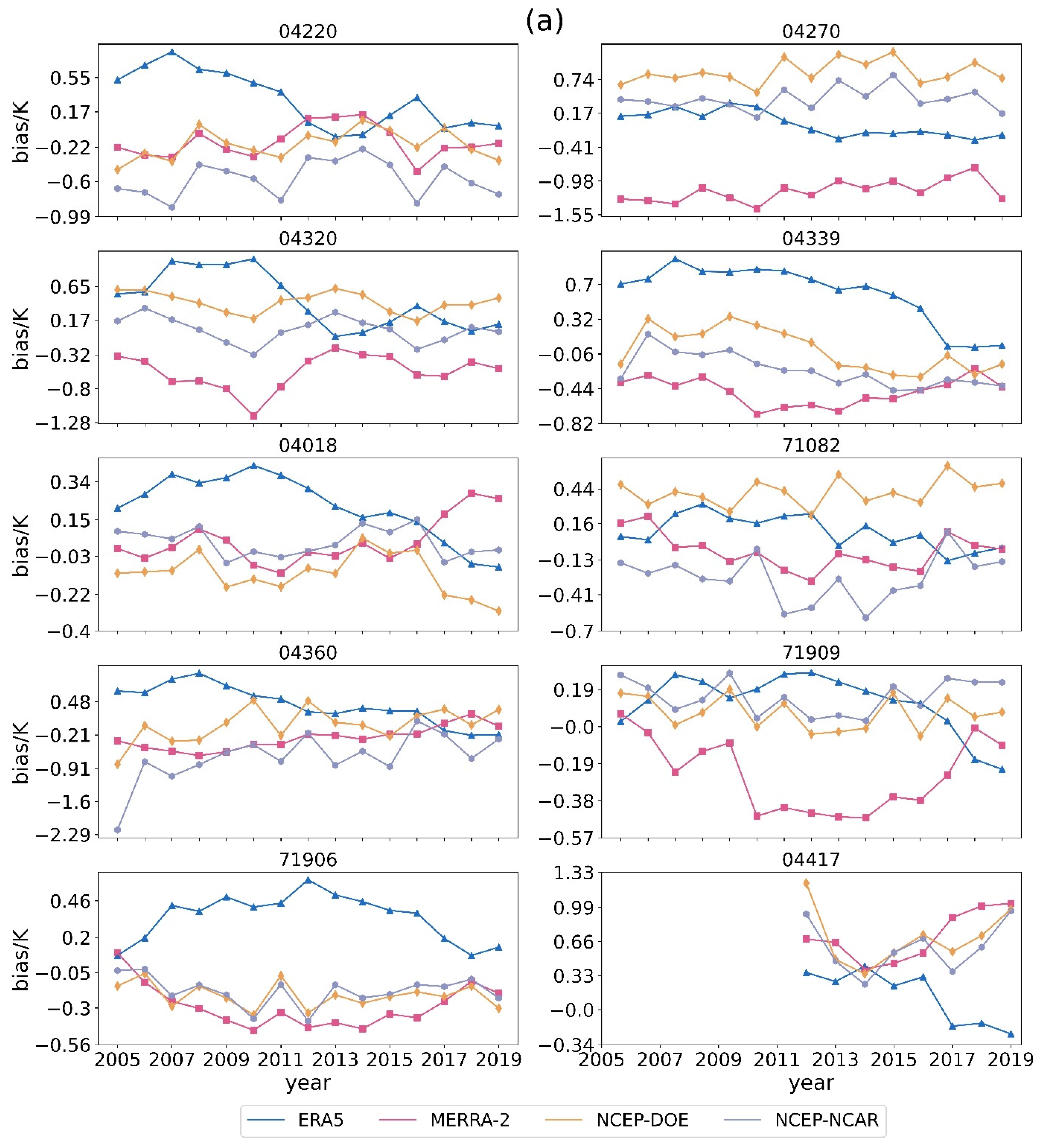
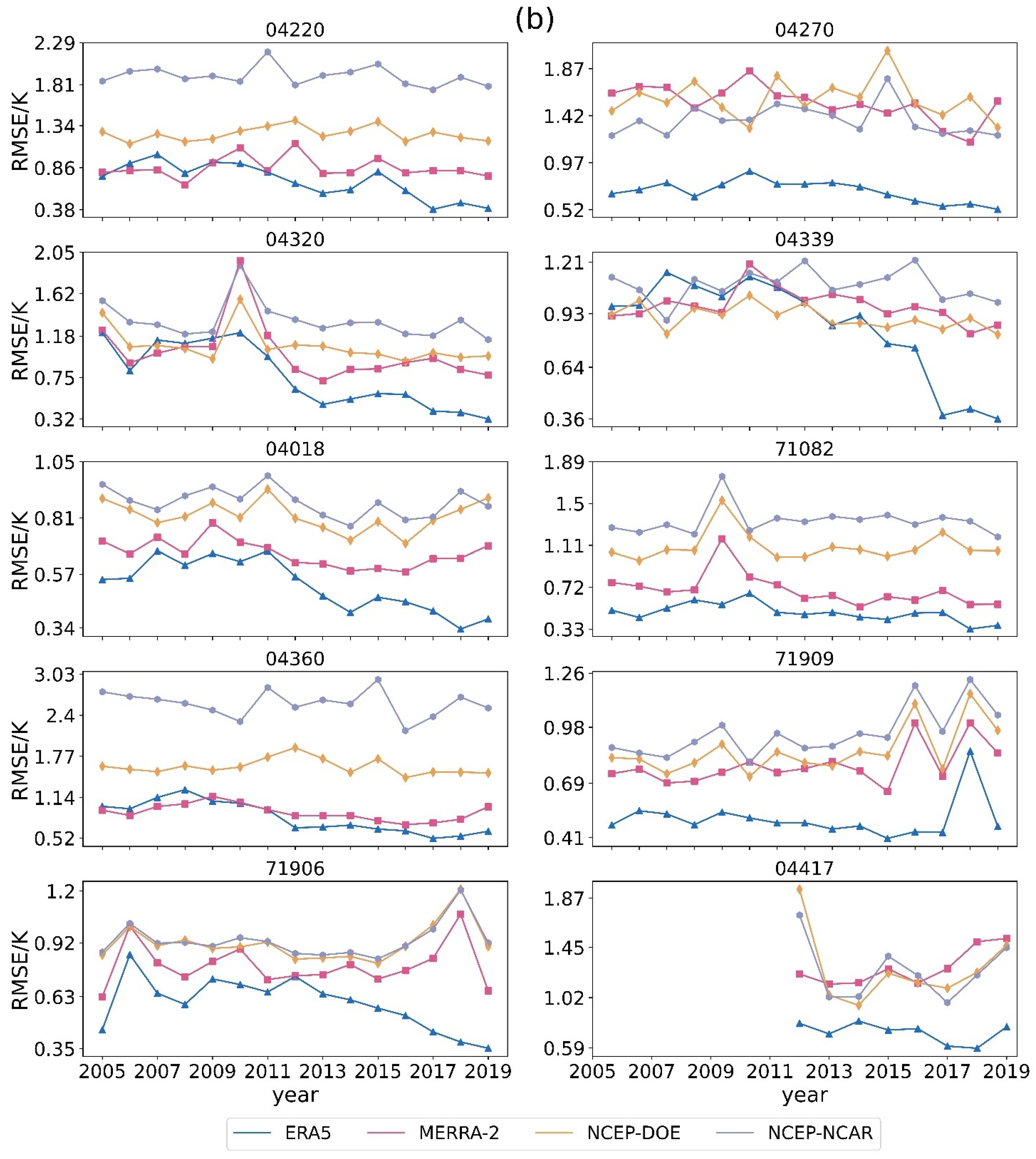
3.2.1. Annual Variation Characteristic

In order to study the annual variation characteristic of the T m , we compute the annual mean bias and the RMSE of the T m from four radiosonde data from 10 radiosonde stations from 2005 to 2019. The results are shown in Figure 3.
The annual mean bias and the RMSE of the ERA5 T m from 2005 to 2019 showed a downward trend in Figure 3, indicating that the accuracy gradually improved. The annual mean bias and the RMSE of the NCEP/DOE T m and the NCEP/NCAR T m consistently varied, and no discernible trend toward greater or worse accuracy was observed, similar to the MERRA-2 T m . The accuracy of the NCEP/DOE T m is better than that of the NCEP/NCAR.
In order to observe the stability and the fluctuation of the annual mean precision variation of the T m , we use four reanalysis data to calculate the mean values and the standard deviation (std) of the annual mean bias and the RMSE of the 10 stations in Greenland from 2005 to 2019. The results are shown in Table 4. The std values of the annual mean bias and the RMSE of the ERA5 T m are 0.32 and 0.22 K, respectively, showing consistent stability. In the MERRA-2, the std values of the annual mean bias and the RMSE are 0.442 and 0.295 K, respectively, at the same level as that of the NCEP/DOE. Meanwhile, the std values of the annual mean bias of the NCEP/DOE and the NCEP/NCAR T m   are relatively close (0.398 and 0.423 K, respectively), while the std of the annual mean RMSE of the NCEP/DOE T m is 0.308 K, which is better than the 0.526 K of NCEP/NCAR. In conclusion, the ERA5 T m has the best inter-annual stability, followed by the NCEP/DOE T m , the MERRA-2 T m , and the NCEP/NCAR T m .

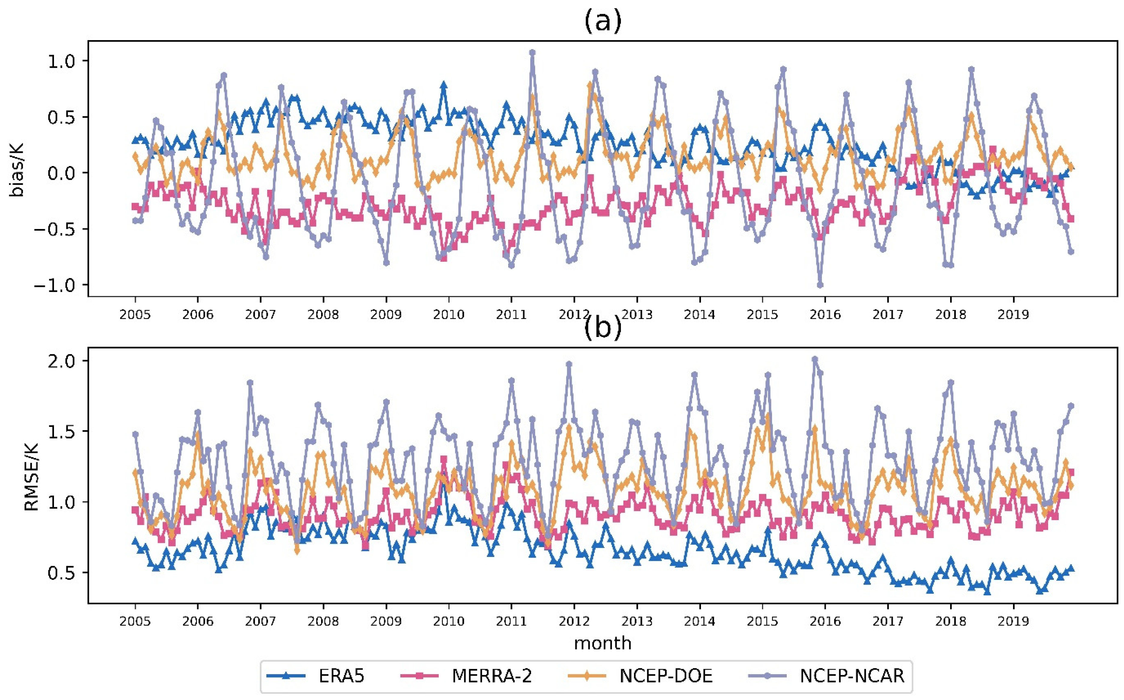
3.2.2. Monthly Variation Characteristic

In order to study the monthly variation characteristic of the T m , we compute the monthly mean bias and the RMSE of the T m from four reanalysis data from 10 radiosonde stations from 2005 to 2019. The results are shown in Figure 4.
The accuracy of the NCEP/NCAR and the NCEP/DOE T m shows obvious seasonal variation characteristics, as follows: the accuracy is better in the summer and poorer in the winter. The accuracy is the best in August and September and the worst in January and December. In addition, a small wave peak in the RMSE occurs in May and June. The accuracy of the ERA5 T m also has a similar, but slighter, seasonal variation; the accuracy in the winter and the spring is worse than that in the summer and the autumn. The seasonal variation of the MERRA-2 T m is similar to the former three, and its volatility is weaker than that of the NCEP/DOE and the NCEP/NCAR T m , and stronger than that of the ERA5 T m . In addition, the accuracy of the ERA5 T m gradually improved from 2005 to 2019. The RMSE from 2005 to 2011 is slightly better than the other three reanalysis data, and its advantages become more obvious from 2012 to 2019, and the RMSE is closer to zero.
In order to explore the physical reasons for the seasonal variation characteristics of the T m accuracy, we check the vertical profiles of the air temperature, the water vapor pressure, and the tropopause height of the reanalysis and radiosonde data (the vertical profiles of the air temperature, water pressure, and tropopause can be found in the Supplemental Material) and find that this may be related to the surface temperature. It can be observed that the difference of tropopause height between the reanalysis and the radiosonde data is not obvious in January and June in terms of quantity and relative relationship. In addition, the water vapor pressures of four reanalysis data have no common differences or changes compared to that of the radiosonde data between January and June.
Bevis et al. [15,45] pointed out that the T m and the Ts have a linear relationship, which means that the accuracy of the Ts will greatly affect the accuracy of the T m . We calculated the T m and Ts at 0:00 and 12:00 every day at 10 stations from 2005 to 2019 in Greenland, and obtained the chart of Ts bias and T m bias compared to those of the radiosonde data. The correlation coefficient between the Ts bias and the T m bias has also been calculated, as shown in Figure A2 of Appendix D. The correlation coefficient between the Ts bias and the T m bias of the ERA5 is 0.248, which is a weak correlation; the value of the MERRA-2 is 0.313, which is a medium correlation; the value of the NCEP/DOE is 0.473, which is a medium correlation; the value of the NCEP/NCAR is 0.538, which is a strong correlation. This means that the accuracy of the T m from these reanalysis data is affected by the Ts to varying degrees.
We counted the mean bias and the RMSE of T m and Ts that were derived from four reanalysis data in the spring (March, April, and May), the summer (June, July, and August), the autumn (September, October, and November), and the winter (December, January, and February). The results are shown in Table 5. It can be observed that the RMSEs of Ts from the four reanalysis models in the winter and spring are greater than that in the summer and autumn, and so are the RMSEs of the T m . Moreover, these are consistent; the size relationship of the correlation coefficient, where the NCAR is the largest, followed by the NCEP/DOE, the MERRA-2, and the ERA5, as well as the value of Ts RMSE, the value of T m RMSE, and the seasonal fluctuation of T m . This may not be a coincidence. We believe that the weaker precision of Ts in the winter and spring than in the summer and autumn, and the strong correlation between the precision of Ts and that of T m , leads to the obvious seasonal variation characteristics of the NCEP/NCAR and the NCEP/DOE T m . The correlation coefficient of the ERA5 and the MERRA-2 is small, and the Ts is slightly weaker in the winter and spring than in the summer and autumn, which leads to their similar seasonal variation characteristics, though not as obvious as the former two. As for why the accuracy of the Ts from the NCEP/DOE and the NCEP/NCAR is lower than that of the ERA5 and the MERRA-2, there may be two aspects, as follows: (1) the assimilation abilities of the NCEP/DOE and the NCEP/NCAR are weaker than the latter two; (2) the horizontal resolution and the vertical resolution are far lower than those of the ERA5 and the MERRA-2, which may lead to larger interpolation errors when interpolating the air temperature to the ground height in order to obtain the Ts.

3.2.3. Daily Variation Characteristic

We used the four reanalysis data and the radiosonde data to calculate the mean T m of the 10 stations at 0:00 and 12:00 each day from 2005 to 2019 in Greenland. In order to make the figure easier to read, and to balance the readability and the amount of information, only the T m in stations 04220, 04270, and 04417 from 2018 to 2019 are shown. The time series plot is shown in Figure 5. The results have consistent seasonal variation, as follows: the T m is higher in the summer and lower in the winter, with the highest point appearing around June and the lowest point emerging in January, and it fluctuates in a sinusoidal curve, which is consistent with the atmospheric temperature variation in the northern hemisphere and can span up to 30–40 K within a year. The ERA5 is close to the calculated results of the radiosonde data. The MERRA-2 results are lower than the results of the radiosonde data most of the time, especially at station 04270. In addition, there is an outlier in the results of ERA5. The bias can reach 5–10 K compared to the result of the radiosonde data on 2 May 2018 in all of the stations. We have checked the ERA5 pressure-level data and have found that it misses a part of the air temperature data for that day.

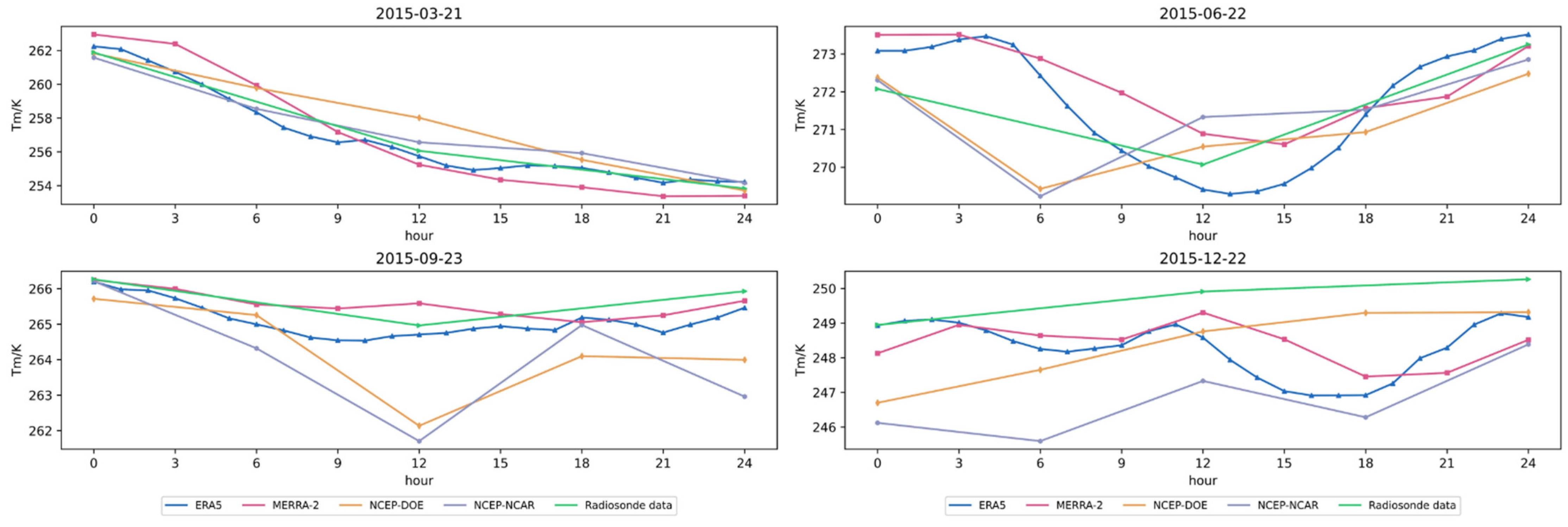
3.2.4. Hourly Variation Characteristic

In practical applications, whether directly using the reanalysis data for calculating the T m or using the reanalysis data to develop a T m model, we focus not only on the general accuracy for more than 10 years, a whole year, a whole month, etc., but also on the performance of the T m at a station in a day even in a moment. According to the above analysis, the accuracy of the T m from the four reanalysis data has certain seasonal variation characteristics. Therefore, the reanalysis data and the radiosonde data are used to calculate the T m of the vernal equinox (21 March), the summer solstice (22 June), the autumn equinox (23 September), and the winter solstice (22 December) in 2015 at the 04220 station, with their highest temporal resolution, respectively. The results are shown in Figure 6. The T m at three time points of 0:00, 12:00, and 24:00, which were calculated by the radiosonde data, are used as reference values in order to evaluate the results of four reanalysis data. The results that were calculated by the ERA5 at these three time points are close to the results of the radiosonde data, and the difference is less than 1 K in most cases. Few moments have almost no difference. Only the difference between 12:00 and 24:00 on the winter solstice exceeds 1 K, at around 1.2–1.5 K. The MERRA-2 results in the spring equinox and the autumnal equinox are close to the radiosonde data, and the difference is within 1 K. Furthermore, the difference at the summer solstice and the winter solstice is larger, especially at 24:00, which is 2–3 K lower than the results of the radiosonde data. The MERRA-2 T m has the same trend as the ERA5 T m . The accuracy of the NCEP/DOE T m is better at the spring equinox and the summer solstice, worse at the autumnal equinox and the winter solstice, and the worst occurs at 12:00 of the autumnal equinox, with bias exceeding −3 K. The NCEP/NCAR has the same trend as the NCEP/DOE, but the bias is larger than that of the NCEP/DOE.
The four reanalysis data have basically the same overall trend in the calculation of the T m from the four dates. However, the reanalysis data with a high temporal resolution, such as the ERA5 and the MERRA-2, can undoubtedly reduce the error that is caused by interpolation to a great extent and efficiently express the temporal variation characteristic of the T m . For example, during the winter solstice, the results of the ERA5 and the NCEP/DOE at 0:00 and 12:00 are similar, but the ERA5 T m from 0:00 to 12:00 has a trend of first falling and then rising. Meanwhile, the NCEP/DOE T m is always rising. If the hourly linear interpolation of the T m that is calculated by the NCEP/DOE is performed, then the maximum difference between the interpolation results and the ERA5 can reach 2 K.
In conclusion, when calculating the T m at a certain point in time, the results of the ERA5 are closest to those that are estimated from the radiosonde data and have a high temporal resolution, which can accurately reflect the variation of the T m over a shorter timescale. Therefore, the ERA5 is the optimal data source for obtaining the T m and for building T m models in a four reanalysis model.

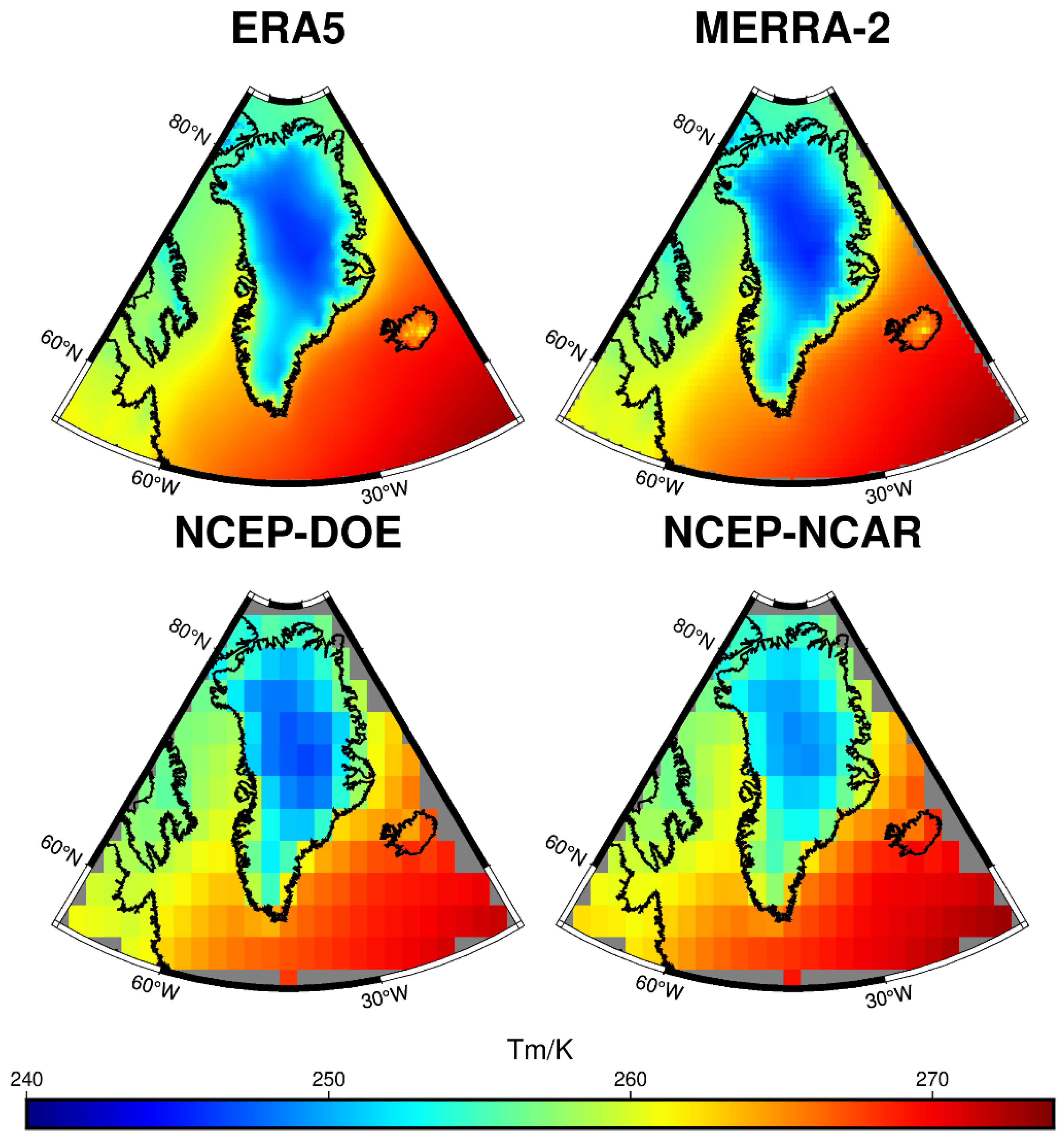
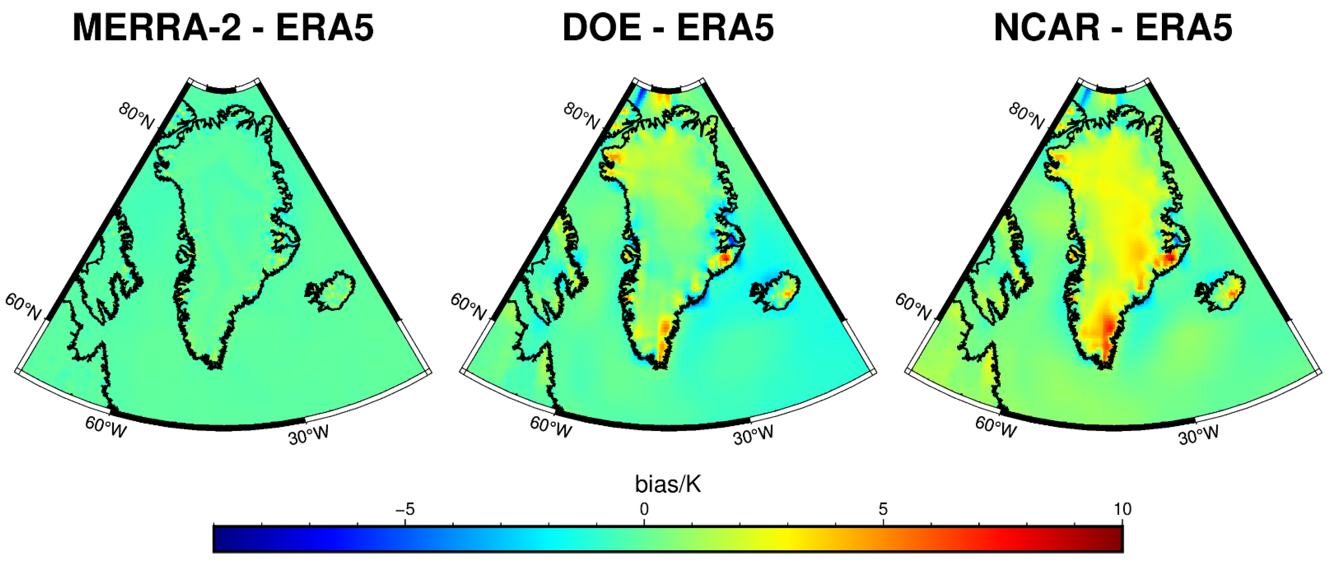
3.3. Spatial Variation of the Performance of Tm Derived from the Four Reanalyses

In order to evaluate the spatial distribution and the variation of the T m in Greenland that were estimated from the four reanalysis data, the mean T m in Greenland from 2005 to 2019 was computed using the four reanalysis data. The results of the three reanalysis data were subtracted from the ERA5 T m in order to observe the spatial differences of the T m . First, the geopotential height of the reanalysis data was converted into geodetic height using the gravity field model. Then, the DEM in Greenland was used as the surface height, and the above four reanalysis data were used to calculate the T m from 2005 to 2019 in Greenland. The results are shown in Figure 7.
In Figure 7, and also according to the DEM map in Figure 1, the results that were computed from the four reanalysis data exhibit a consistent distribution, as follows: the T m is proportional to the ground elevation, and the greater the ground elevation, the lower the T m . In the middle region of Greenland, the ground elevation is higher, and the T m is lower, whereas the height at the island’s edge is lower, and the T m is higher, which conforms to the definition formula for the T m . The results of the ERA5 are between 245.7 and 273.2 K in Greenland from 2005 to 2019; the results of the MERRA-2 are between 243.9 and 272 K, which is less than that of the ERA5 T m ; the results of the NCEP/DOE are between 246.2 and 272.9 K, which is comparable to the ERA5 T m ; and the results of the NCEP/NCAR are between 248.6 and 273.5 K, which is greater than that of the ERA5. Furthermore, the ERA5, with a high spatial resolution, can more precisely reflect the distribution of the T m on steep terrains that are in a small area, such as glaciers, ice sheets, mountain glaciers, and U-shaped valleys and fjords. The previous analysis demonstrates that the accuracy of the ERA5 is the highest. Accordingly, the results of the ERA5 are used as a reference. The 15-year mean T m that was obtained from the other three reanalysis is interpolated to the spatial resolution of the ERA5 and subtracted by the result of the ERA5 in order to determine the regional difference for the T m between the four reanalysis data, as illustrated in Figure 8.
The overall difference between the MERRA-2 T m and the ERA5 T m is relatively uniform in the whole area, generally around −2 K, which is lower than the ERA5 T m by around 2 K, as shown in Figure 8. In the central area of Greenland, the difference is larger, reaching around −3 K. The difference between the NCEP/DOE T m and the ERA5 T m is mainly concentrated in the edge area of the island, which is higher than the ERA5 T m by more than 5 K. The possible reason for this is that the difference between the land and the sea results in large errors in interpolation. The difference between the NCEP/NCAR T m and the ERA5 T m is relatively large on the whole island, which is generally higher than the ERA5 T m by more than 2.5 K. In the south and the southeast of Greenland, two large areas have large differences, which are higher than the ERA5 T m by more than 5 K.

4. Conclusions

In this work, we use the ERA5, the MERRA-2, the NCEP/DOE, and the NCEP/NCAR to calculate the T m in Greenland from 2005 to 2019 and employ the radiosonde data of 10 stations in order to evaluate the accuracy and the spatial–temporal variation of the T m that is derived from four reanalysis data. The following conclusions have been obtained:
  • The ERA5 is the best in terms of the overall accuracy. The 15-year MBE and the RMSE of the ERA5 T m are 0.267 and 0.691 K, respectively. In the MERRA-2 T m , the MBE and the RMSE are −0.247 and 0.962 K, respectively. In the NCEP/DOE T m , the MBE and the RMSE are 0.192 and 1.148 K, respectively. The NCEP/NCAR T m is the worst, with an MBE and RMSE of −0.069 and 1.37 K, respectively. The error of the ERA5 T m corresponds to an uncertainty of 0.26% in the PWV, while this is 0.36% for the MERRA2, 0.43% for the NCEP/DOE, and 0.52% for the NCEP/NCAR. The ERA5 is the best data source for the direct determination of accurate T m and the development of T m models in Greenland;
  • In terms of the inter-annual stability of the calculation accuracy, the ERA5 T m is the most stable, followed by the NCEP/DOE T m , the MERRA-2 T m , and the NCEP/NCAR T m . The accuracy of the ERA5 T m has been improving from 2005 to 2019. Meanwhile, the accuracy of the NCEP/NCAR T m and the NCEP/DOE T m has the following seasonal variation characteristics: better accuracy in the summer and autumn and poorer accuracy in the winter and spring; the ERA5 T m and the MERRA-2 T m are similar to the former two, but less obviously. There is a relatively strong correlation between the accuracy of the Ts and that of the T m that are derived from the four reanalysis models, especially the NCEP/NCAR. The weaker precision of the Ts in the winter and spring than that of the summer and autumn leads to the obvious seasonal variation characteristics of T m precision. When calculating the T m by hour, the results of the ERA5 are the closest to those that were estimated from the radiosonde data and have a high temporal resolution, which can accurately reflect the variation of the T m over a shorter timescale;
  • In the spatial distribution of the T m , the results of the four reanalysis data are generally consistent; the central area of Greenland is smaller, and the edge of the island is larger. In comparison with the ERA5, the overall difference between the MERRA2 and the ERA5 is about −2 K. Meanwhile, the difference between the NCEP/DOE and the ERA5 is mainly concentrated on the edge of the island; the difference between the NCEP/NCAR and the ERA5 is relatively large on the whole island, especially in the south and the southeast.

Supplementary Materials

The following supporting information can be downloaded at: https://www.mdpi.com/article/10.3390/rs14215431/s1, Figure S1: Air temperature of four reanalysis and radiosonde data in station 04270 in January and July 2019; Figure S2: Water vapor pressure of four reanalysis and radiosonde data in station 04270 in January and July 2019.

Author Contributions

S.Z., F.X., and L.G.: study idea and experimental program design; C.L., L.G., F.X., J.L., W.L. and S.Z.: data processing and management; C.L.: preparation of the original draft; S.Z., L.G. and F.X.: paper review and editing. All authors have read and agreed to the published version of the manuscript.

Funding

This work was supported in part by the National Key Research and Development Program of China under Grant 2017YFA0603104 and in part by the Natural Science Foundation of China under Grant 41730102.

Data Availability Statement

The ERA5 data were obtained from ECMWF (https://www.ecmwf.int/en/forecasts/datasets/reanalysis-datasets/era5 (accessed on 16 July 2022)), and the MERRA-2 data were acquired from NASA (https://disc.gsfc.nasa.gov/datasets?project=MERRA-2 (accessed on 16 July 2022)). The NCEP/NCAR data were obtained from NOAA Physical Sciences Laboratory (PSL) (https://psl.noaa.gov/data/gridded/data.ncep.reanalysis.html (accessed on 16 July 2022)), and the NCEP/DOE data were acquired from PSL (https://psl.noaa.gov/data/gridded/data.ncep.reanalysis2.html (accessed on 16 July 2022)). Meanwhile, the radiosonde data were obtained from the University of Wyoming (http://weather.uwyo.edu/upperair/np.html (accessed on 16 July 2022)). The DEM was obtained from ETOPO1 (DEM is provided by EROPO1(https://ngdc.noaa.gov/mgg/global/global.html (accessed on 16 July 2022)). The T m estimates can be obtained from the corresponding author upon reasonable request.

Acknowledgments

We are grateful to ECMWF, NASA, PSL, and the University of Wyoming for providing relevant data.

Conflicts of Interest

The authors declare no conflict of interest.

Appendix A

1. Xu et al. [46] studied the error of the saturation water vapor pressure that was calculated by using different formulas compared with Goff–Gratch and found that the Magnus formula has a simple calculation form and a high accuracy. Accordingly, we use the Magnus formula over water to calculate the saturation water vapor pressure of the radiosonde data, the NCEP/NCAR, and the NCEP/DOE. The Magnus formula is as follows [47]:
e s ( T i ) = 6.11 × 10 ( 7.5 × T i 237.3 + T i ) ,
where T is in °C.
2. Luo et al. [48] claim that the MERRA-2 and the ERA-Interim relative humidity algorithms employed a modified version of Teten’s formula [49]. The ERA-Interim is the previous generation’s reanalysis product of ERA5, in which they use the same formula to calculate the saturation water vapor pressure [50].Thus, we use the Teten’s formula that has been modified by Simmons et al. [49] to calculate the saturation water vapor pressure of the ERA5 and the MERRA-2, which has the following three forms: over water when T 273.16 K, over ice when T 250.16 K, and a mixed formula between 250.16 and 273.16 K, as follows:
e s ( T i ) = α e s ( w a t e r ) ( T i ) + ( 1 α ) e s ( i c e ) ( T i ) ,
where α is the coefficient, and its formula is as follows, e s ( w a t e r ) and   e s ( i c e ) are the saturation water vapor pressure over water and ice, respectively, and their formula is presented in Equation (A4).
α = { 0 , T i T ice ( T i T ice T 0 T ice ) 2 , T ice < T i < T 0 1 , T i T 0 ,
where   T ice   = 250.16 K, and T 0   = 273.16 K.
e s ( w a t e r   o r   i c e ) ( T i ) = a 1 e a 2 ( T i 273.16 T i a 3 )
where e s ( w a t e r   o r   i c e ) represents the saturation water vapor pressure over water or ice, and T i is in K. When calculating the saturation water vapor pressure over water, a 1 = 611.21 Pa, a 2 = 17.502, and a 3 = 32.19 K. When calculating the saturation water vapor pressure over ice, a 1 = 611.21 Pa, a 2 = 22.587, and a 3 = −0.7 K.

Appendix B

Figure A1. Tm derived from four reanalysis and radiosonde data under different heights (ground height of the station, 925, 850, 700, 600, 500, 400, and 300 hPa) and the tropopause.
Remotesensing 14 05431 g0a1

Appendix C

Bevis et al. [15] derive the formula of connecting ZWD and PWV as follows:
P W V =   Π · Z W D ,
where Π is the following conversion parameter:
Π   = 10 6 ρ R v · ( k 3 T m + k 2 )   ,
where R v is the specific gas constant for water vapor, ρ is density of liquid water. R v = 0.462   J   ·   g 1   ·   K 1 , ρ = 1   g / cm 3 , k 2 = 16.581   K / hPa , and k 3 = 3.776     10 5   K 2 / hPa .
( P W V ) T m = ( k 3 k 3 + k 2 T m ) P W V T m ,
where R v is the specific gas constant for water vapor, ρ is density of liquid water. R v = 0.462   J   ·   g 1   ·   K 1 , ρ = 1   g / cm 3 , k 2 = 16.581   K / hPa , and k 3 = 3.776     10 5   K 2 / hPa .
S = ( P W V ) P W V T m T m = k 3 k 3 + k 2 T m = 1 1 + k 2 k 3 T m     1 ,
where S is the relative sensitivity, since k 2 k 3 = 4.39     10 5   K 1 , it is very small, thus S     1 .

Appendix D

Figure A2. Ts bias and Tm bias of four reanalysis models from 2005 to 2019 at 10 stations in Greenland.
Remotesensing 14 05431 g0a2

References

  1. Bamber, J.L.; Layberry, R.L.; Gogineni, S.P. A New Ice Thickness and Bed Data Set for the Greenland Ice Sheet: 1. Measurement, Data Reduction, and Errors. J. Geophys. Res. Atmos. 2001, 106, 33773–33780. [Google Scholar] [CrossRef]
  2. Lythe, M.B.; Vaughan, D.G. BEDMAP: A New Ice Thickness and Subglacial Topographic Model of Antarctica. J. Geophys. Res. Solid Earth 2001, 106, 11335–11351. [Google Scholar] [CrossRef] [Green Version]
  3. Hu, A.; Meehl, G.A.; Han, W.; Yin, J. Effect of the Potential Melting of the Greenland Ice Sheet on the Meridional Overturning Circulation and Global Climate in the Future. Deep Sea Res. Part II Top. Stud. Oceanogr. 2011, 58, 1914–1926. [Google Scholar] [CrossRef]
  4. Chung, E.S.; Soden, B.; Sohn, B.J.; Shi, L. Upper-tropospheric moistening in response to anthropogenic warming. Proc. Natl. Acad. Sci. USA 2014, 111, 11636–11641. [Google Scholar] [CrossRef] [Green Version]
  5. Lee, S.; Gong, T.; Feldstein, S.B.; Screen, J.A.; Simmonds, I. Revisiting the Cause of the 1989–2009 Arctic Surface Warming Using the Surface Energy Budget: Downward Infrared Radiation Dominates the Surface Fluxes. Geophys. Res. Lett. 2017, 44, 10654–10661. [Google Scholar] [CrossRef]
  6. Sato, K.; Simmonds, I. Antarctic Skin Temperature Warming Related to Enhanced Downward Longwave Radiation Associated with Increased Atmospheric Advection of Moisture and Temperature. Environ. Res. Lett. 2021, 16, 064059. [Google Scholar] [CrossRef]
  7. Gaffen, D.J.; Sargent, M.A.; Habermann, R.E.; Lanzante, J.R. Sensitivity of Tropospheric and Stratospheric Temperature Trends to Radiosonde Data Quality. J. Clim. 2000, 13, 1776–1796. [Google Scholar] [CrossRef]
  8. Hagemann, S.; Bengtsson, L.; Gendt, G. On the Determination of Atmospheric Water Vapor from GPS Measurements. J. Geophys. Res. Atmos. 2003, 108, 4678. [Google Scholar] [CrossRef] [Green Version]
  9. Champollion, C.; Masson, F.; Van Baelen, J.; Walpersdorf, A.; Chéry, J.; Doerflinger, E. GPS Monitoring of the Tropospheric Water Vapor Distribution and Variation during the 9 September 2002 Torrential Precipitation Episode in the Cévennes (Southern France). J. Geophys. Res. Atmos. 2004, 109, D24102. [Google Scholar] [CrossRef] [Green Version]
  10. Yuan, Y.; Zhang, K.; Rohm, W.; Choy, S.; Norman, R.; Wang, C.-S. Real-Time Retrieval of Precipitable Water Vapor from GPS Precise Point Positioning. J. Geophys. Res. Atmos. 2014, 119, 10044–10057. [Google Scholar] [CrossRef]
  11. Zhao, Q.; Yao, Y.; Yao, W. GPS-Based PWV for Precipitation Forecasting and Its Application to a Typhoon Event. J. Atmos. Sol. Terr. Phys. 2018, 167, 124–133. [Google Scholar] [CrossRef]
  12. Guo, M.; Zhang, H.; Xia, P. Exploration and Analysis of the Factors Influencing GNSS PWV for Nowcasting Applications. Adv. Space Res. 2021, 67, 3960–3978. [Google Scholar] [CrossRef]
  13. Davis, J.L.; Herring, T.A.; Shapiro, I.I.; Rogers, A.E.E.; Elgered, G. Geodesy by Radio Interferometry: Effects of Atmospheric Modeling Errors on Estimates of Baseline Length. Radio Sci. 1985, 20, 1593–1607. [Google Scholar] [CrossRef]
  14. Askne, J.; Nordius, H. Estimation of Tropospheric Delay for Microwaves from Surface Weather Data. Radio Sci. 1987, 22, 379–386. [Google Scholar] [CrossRef]
  15. Bevis, M.; Businger, S.; Herring, T.A.; Rocken, C.; Anthes, R.A.; Ware, R.H. GPS Meteorology: Remote Sensing of Atmospheric Water Vapor Using the Global Positioning System. J. Geophys. Res. Atmos. 1992, 97, 15787–15801. [Google Scholar] [CrossRef]
  16. Ross, R.J.; Rosenfeld, S. Estimating Mean Weighted Temperature of the Atmosphere for Global Positioning System Applications. J. Geophys. Res. Atmos. 1997, 102, 21719–21730. [Google Scholar] [CrossRef] [Green Version]
  17. Yao, Y.; Xu, C.; Zhang, B.; Cao, N. GTm-III: A New Global Empirical Model for Mapping Zenith Wet Delays onto Precipitable Water Vapour. Geophys. J. Int. 2014, 197, 202–212. [Google Scholar] [CrossRef] [Green Version]
  18. Böhm, J.; Möller, G.; Schindelegger, M.; Pain, G.; Weber, R. Development of an Improved Empirical Model for Slant Delays in the Troposphere (GPT2w). GPS Solut. 2015, 19, 433–441. [Google Scholar] [CrossRef] [Green Version]
  19. Landskron, D.; Böhm, J. VMF3/GPT3: Refined Discrete and Empirical Troposphere Mapping Functions. J. Geod. 2018, 92, 349–360. [Google Scholar] [CrossRef]
  20. VMF. Data Server—Products. Available online: https://vmf.geo.tuwien.ac.at/products.html (accessed on 24 September 2022).
  21. Boehm, J.; Werl, B.; Schuh, H. Troposphere Mapping Functions for GPS and Very Long Baseline Interferometry from European Centre for Medium-Range Weather Forecasts Operational Analysis Data. J. Geophys. Res. Solid Earth 2006, 111. [Google Scholar] [CrossRef]
  22. Boehm, J.; Kouba, J.; Schuh, H. Forecast Vienna Mapping Functions 1 for Real-Time Analysis of Space Geodetic Observations. J. Geod. 2009, 83, 397–401. [Google Scholar] [CrossRef]
  23. He, C.; Wu, S.; Wang, X.; Hu, A.; Wang, Q.; Zhang, K. A New Voxel-Based Model for the Determination of Atmospheric Weighted Mean Temperature in GPS Atmospheric Sounding. Atmos. Meas. Tech. 2017, 10, 2045–2060. [Google Scholar] [CrossRef] [Green Version]
  24. Sun, Z.; Zhang, B.; Yao, Y. A Global Model for Estimating Tropospheric Delay and Weighted Mean Temperature Developed with Atmospheric Reanalysis Data from 1979 to 2017. Remote Sens. 2019, 11, 1893. [Google Scholar] [CrossRef] [Green Version]
  25. Sun, Z.; Zhang, B.; Yao, Y. An ERA5-Based Model for Estimating Tropospheric Delay and Weighted Mean Temperature Over China With Improved Spatiotemporal Resolutions. Earth Space Sci. 2019, 6, 1926–1941. [Google Scholar] [CrossRef]
  26. Ma, Y.; Chen, P.; Liu, T.; Xu, G.; Lu, Z. Development and Assessment of an ALLSSA-Based Atmospheric Weighted Mean Temperature Model With High Time Resolution for GNSS Precipitable Water Retrieval. Earth Space Sci. 2022, 9, e2021EA002089. [Google Scholar] [CrossRef]
  27. Wang, J.; Zhang, L.; Dai, A. Global Estimates of Water-Vapor-Weighted Mean Temperature of the Atmosphere for GPS Applications. J. Geophys. Res. Atmos. 2005, 110. [Google Scholar] [CrossRef] [Green Version]
  28. Zhang, W.; Zhang, H.; Liang, H.; Lou, Y.; Cai, Y.; Cao, Y.; Zhou, Y.; Liu, W. On the Suitability of ERA5 in Hourly GPS Precipitable Water Vapor Retrieval over China. J. Geod. 2019, 93, 1897–1909. [Google Scholar] [CrossRef]
  29. Guo, L.; Huang, L.; Li, J.; Liu, L.; Huang, L.; Fu, B.; Xie, S.; He, H.; Ren, C. A Comprehensive Evaluation of Key Tropospheric Parameters from ERA5 and MERRA-2 Reanalysis Products Using Radiosonde Data and GNSS Measurements. Remote Sens. 2021, 13, 3008. [Google Scholar] [CrossRef]
  30. Tang, G.; Long, D.; Behrangi, A.; Wang, C.; Hong, Y. Exploring Deep Neural Networks to Retrieve Rain and Snow in High Latitudes Using Multisensor and Reanalysis Data. Water Resour. Res. 2018, 54, 8253–8278. [Google Scholar] [CrossRef] [Green Version]
  31. Jiang, P.; Ye, S.; Chen, D.; Liu, Y.; Xia, P. Retrieving Precipitable Water Vapor Data Using GPS Zenith Delays and Global Reanalysis Data in China. Remote Sens. 2016, 8, 389. [Google Scholar] [CrossRef]
  32. Jade, S.; Vijayan, M.S.M. GPS-Based Atmospheric Precipitable Water Vapor Estimation Using Meteorological Parameters Interpolated from NCEP Global Reanalysis Data. J. Geophys. Res. Atmos. 2008, 113, D03106. [Google Scholar] [CrossRef] [Green Version]
  33. Li, M.; Wu, P.; Ma, Z. A Comprehensive Evaluation of Soil Moisture and Soil Temperature from Third-Generation Atmospheric and Land Reanalysis Data Sets. Int. J. Climatol. 2020, 40, 5744–5766. [Google Scholar] [CrossRef]
  34. Hersbach, H.; Bell, B.; Berrisford, P.; Hirahara, S.; Horányi, A.; Muñoz-Sabater, J.; Nicolas, J.; Peubey, C.; Radu, R.; Schepers, D.; et al. The ERA5 Global Reanalysis. Q. J. R. Meteorol. Soc. 2020, 146, 1999–2049. [Google Scholar] [CrossRef]
  35. Gelaro, R.; McCarty, W.; Suárez, M.J.; Todling, R.; Molod, A.; Takacs, L.; Randles, C.A.; Darmenov, A.; Bosilovich, M.G.; Reichle, R.; et al. The Modern-Era Retrospective Analysis for Research and Applications, Version 2 (MERRA-2). J. Clim. 2017, 30, 5419–5454. [Google Scholar] [CrossRef] [PubMed]
  36. Kalnay, E.; Kanamitsu, M.; Kistler, R.; Collins, W.; Deaven, D.; Gandin, L.; Iredell, M.; Saha, S.; White, G.; Woollen, J.; et al. The NCEP/NCAR 40-Year Reanalysis Project. Bull. Am. Meteorol. Soc. 1996, 77, 437–472. [Google Scholar] [CrossRef]
  37. NOAA Physical Sciences Laboratory. NCEP-NCAR Reanalysis 1. Available online: https://psl.noaa.gov/data/gridded/data.ncep.reanalysis.html (accessed on 16 July 2022).
  38. Kanamitsu, M.; Ebisuzaki, W.; Woollen, J.; Yang, S.-K.; Hnilo, J.J.; Fiorino, M.; Potter, G.L. NCEP–DOE AMIP-II Reanalysis (R-2). Bull. Am. Meteorol. Soc. 2002, 83, 1631–1644. [Google Scholar] [CrossRef] [Green Version]
  39. NOAA Physical Sciences Laboratory. NCEP/DOE Reanalysis II. Available online: https://psl.noaa.gov/data/gridded/data.ncep.reanalysis2.html (accessed on 16 July 2022).
  40. McIlveen, R. Fundamentals of Weather and Climate; Psychology Press: London, UK, 1991; ISBN 978-0-7487-4079-6. [Google Scholar]
  41. WMO. Guide to Meteorological Instruments and Methods of Observation; WMO: Geneva, Switzerland, 1996. [Google Scholar]
  42. Mahoney, M. A Discussion of Various Measures of Altitude, Jet Propulsion Laboratory. MTP Altitude Discussion. 2001. Available online: https://wahiduddin.net/calc/refs/measures_of_altitude_mahoney.html (accessed on 19 July 2022).
  43. World Meteorological Organization (WMO). Meteorology A Three-Dimensional Science: Second Session of the Commission for Aerology; WMO Bulletin IV(4); WMO: Geneva, Switzerland, 1957; pp. 134–138. [Google Scholar]
  44. Davis, P.J. Interpolation and Approximation; Courier Corporation: North Chelmsford, MA, USA, 1975; ISBN 978-0-486-62495-2. [Google Scholar]
  45. Bevis, M.; Businger, S.; Chiswell, S.; Herring, T.A.; Anthes, R.A.; Rocken, C.; Ware, R.H. GPS Meteorology: Mapping Zenith Wet Delays onto Precipitable Water. J. Appl. Meteorol. 1994, 33, 379–386. [Google Scholar] [CrossRef]
  46. Junzeng, X.; Qi, W.; Shizhang, P.; Yanmei, Y. Error of Saturation Vapor Pressure Calculated by Different Formulas and Its Effect on Calculation of Reference Evapotranspiration in High Latitude Cold Region. Procedia Eng. 2012, 28, 43–48. [Google Scholar] [CrossRef] [Green Version]
  47. Murray, F.W. On the Computation of Saturation Vapor Pressure. J. Appl. Meteorol. Climatol. 1967, 6, 203–204. [Google Scholar] [CrossRef]
  48. Luo, B.; Minnett, P.J.; Szczodrak, M.; Nalli, N.R.; Morris, V.R. Accuracy Assessment of MERRA-2 and ERA-Interim Sea Surface Temperature, Air Temperature, and Humidity Profiles over the Atlantic Ocean Using AEROSE Measurements. J. Clim. 2020, 33, 6889–6909. [Google Scholar] [CrossRef]
  49. Simmons, A.J.; Untch, A.; Jakob, C.; Kållberg, P.; Undén, P. Stratospheric Water Vapour and Tropical Tropopause Temperatures in Ecmwf Analyses and Multi-year Simulations. Q. J. R. Meteorol. Soc. 1999, 125, 353–386. [Google Scholar] [CrossRef]
  50. ECMWF. IFS Documentation CY41R2—Part IV: Physical Processes. Available online: https://www.ecmwf.int/en/elibrary/16648-ifs-documentation-cy41r2-part-iv-physical-processes (accessed on 16 July 2022).
Figure 1. Distribution of 10 radiosonde stations in Greenland and the surrounding areas.
Remotesensing 14 05431 g001
Figure 2. The 15-year mean (a) bias and (b) RMSE for the T m of 10 stations derived from four reanalyses.
Remotesensing 14 05431 g002
Figure 3. Annual mean (a) bias and (b) RMSE of T m at 10 stations from 2005 to 2019 calculated from four reanalysis data.
Remotesensing 14 05431 g003aRemotesensing 14 05431 g003b
Figure 4. Monthly mean (a) bias and (b) RMSE of T m of 10 stations from 2005 to 2019 calculated from four reanalysis data.
Remotesensing 14 05431 g004
Figure 5. Time series plot for T m in stations 04220, 04270, and 04417, from 2018 to 2019.
Remotesensing 14 05431 g005
Figure 6. T m of the vernal equinox, summer solstice, autumn equinox, and winter solstice in 2005 at station 04220, with the highest temporal resolution from the four reanalysis data.
Remotesensing 14 05431 g006
Figure 7. Mean T m computed from the four reanalysis data in Greenland from 2005 to 2019.
Remotesensing 14 05431 g007
Figure 8. Regional T m differences between MERRA-2, NCEP/DOE, NCEP/NCAR, and ERA5 in Greenland.
Remotesensing 14 05431 g008
Table 1. Basic information of the four reanalysis data.
ERA5MERRA-2NCEP/NCARNCEP/DOE
SourceECMWFNASANCEP, NCARNCEP, DOE
Temporal coverage1950–present1980–present1948–present1979–present
Release time2016201419952001
Temporal resolution1 h3 h6 h6 h
Assimilation scheme4D-VAR3D-VAR3D-VAR3D-VAR
Horizontal resolution (latitude × longitude)0.25° × 0.25°0.5° × 0.625°2.5° × 2.5°2.5° × 2.5°
Vertical resolution37 pressure levels (from 1000 to 1 hPa)42 pressure levels (from 1000 to 0.1 hPa)17 pressure levels (from 1000 to 10 hPa)17 pressure levels (from 1000 to 10 hPa)
The number of pressure levels below 300 hPa202188
Table 2. Spatial information of 10 radiosonde stations.
Radiosonde StationLatitude (°N)Longitude (°)Geopotential Height (m)The Mean Number of
Pressure Levels Below 300 hPa
from 2005 to 2019 (Mean ± Std)
7190658.1167−68.416760.262.9 ± 23.7
427061.1667−45.416734.057.3 ± 17.6
7190963.7500−68.550021.970.6 ± 21.8
401863.9806−22.595052.043.5 ± 16.6
436065.6111−37.636754.036.7 ± 20.0
422068.7081−52.851743.055.7 ± 16.8
433970.4844−21.951170.027.7 ± 9.7
441772.5700−38.45003255.025.3 ± 10.1
432076.7694−18.668111.055.9 ± 15.7
7108282.5000−62.333365.462.0 ± 20.0
Table 3. The 15-year mean bias and RMSE values for the T m of 10 stations derived from four reanalyses.
SiteERA5MERRA-2NCEP/DOENCEP/NCAR
Bias (K)RMSE (K)Bias (K)RMSE (K)Bias (K)RMSE (K)Bias (K)RMSE (K)
042200.3040.735−0.1550.867−0.1991.249−0.5631.909
04270−0.0130.702−1.1521.5550.8621.5920.4111.385
043200.4510.833−0.5571.050.4261.0930.0361.351
043390.6000.896−0.4720.978−0.0170.912−0.2421.087
040180.2170.5330.0440.661−0.1170.8220.0380.88
710820.0960.491−0.0650.7120.4131.106−0.2741.342
043600.4170.867−0.2830.92−0.0011.616−0.6772.585
719090.1240.516−0.2490.7890.070.8680.1530.957
719060.3440.608−0.2880.807−0.2110.923−0.1790.935
044170.1340.7280.7061.2840.6981.2990.6021.273
Mean0.2670.691−0.2470.9620.1921.148−0.0691.37
Min−0.0130.491−1.1520.661−0.2110.822−0.6770.88
Max0.6000.8960.7061.5550.8621.6160.6022.585
Table 4. Mean values and standard deviation of the annual mean bias and RMSE of T m derived from four reanalysis data from 2005 to 2019.
Reanalysis DataAnnual Mean BiasAnnual Mean RMSE
Mean (K)Std (K)Mean (K)Std (K)
ERA50.2670.3180.6660.226
MERRA-2−0.2470.4420.9350.295
NCEP/DOE0.1920.3981.1330.308
NCEP/NCAR−0.0690.4231.3680.526
Table 5. Mean bias and RMSE values for T m and Ts derived from four reanalysis data in different seasons.
SeasonERA5MERRA-2NCEP/DOENCEP/NCAR
Bias (K)RMSE (K)Bias (K)RMSE (K)Bias (K)RMSE (K)Bias (K)RMSE (K)
T m Spring0.2190.646−0.2470.9380.3701.1000.3081.273
Summer0.2460.655−0.2530.8170.1300.9140.3131.039
Autumn0.2340.648−0.2350.8910.0651.100−0.3891.375
Winter0.3100.726−0.3511.0090.1021.213−0.5101.507
TsSpring0.2901.6570.0341.7131.1543.4240.3303.175
Summer0.6711.7900.3111.6821.8422.9381.7772.831
Autumn−0.2101.291−0.3421.286−0.9402.543−2.2853.367
Winter−0.1961.627−0.3721.841−1.1693.398−3.9505.149
Publisher’s Note: MDPI stays neutral with regard to jurisdictional claims in published maps and institutional affiliations.

